Injection of Deformable Capsules in a Reservoir: A Systematic Analysis


1
School of Engineering, Università della Basilicata, Viale dell’Ateneo Lucano 10, 85100 Potenza, Italy
2
Centro di Eccellenza in Meccanica Computazionale (CEMeC), Politecnico di Bari, Via Re David 200-70125 Bari, Italy
3
Department of Mechanical Engineering, University of Bristol, Bristol BS8 1TH, UK
*
Author to whom correspondence should be addressed.
Fluids 2019, 4(3), 122; https://doi.org/10.3390/fluids4030122
Submission received: 29 May 2019
/
Revised: 25 June 2019
/
Accepted: 27 June 2019
/
Published: 3 July 2019
(This article belongs to the Special Issue Cardiovascular Flows)
Abstract
:Motivated by red blood cell dynamics and injectable capsules for drug delivery, in this paper, a computational study of capsule ejection from a narrow channel into a reservoir is undertaken for a combination of varying deformable capsule sizes and channel dimensions. A mass-spring membrane model is coupled to an Immersed Boundary–Lattice Boltzmann model solver. The aim of the present work is the description of the capsules’ motion, deformation and the response of the fluid due to the complex particles’ dynamics. The interactions between the capsules affect the local velocity field and are responsible for the dynamics observed. Capsule membrane deformability is also seen to affect inter-capsule interaction. We observe that the train of three particles locally homogenises the velocity field and the leading capsule travels faster than the other two trailing capsules. Variations in the size of reservoir do not seem to be relevant, while the ratio of capsule diameter to channel diameter as well as the ratio of capsule diameter to inter-capsule spacing play a major role. This flow set-up has not been covered in the literature, and consequently we focus on describing capsule motion, membrane deformation and fluid dynamics, as a preliminary investigation in this field.
1. Introduction
Haemodynamcis in large arteries is commonly described by the incompressible Newtonian Navier–Stokes equations, hence modelling whole blood to have a constant density and viscosity. While this is acceptable for larger arteries at high flow rates, it is more appropriate to adopt a thixotropic non-Newtonian shear-thinning rheological model for viscosity when a larger variation of shear rates is apparent as evident in smaller vessels or slower flows. This would then take into account the presence of the erythrocytes and other constituents of whole blood [1,2] in a continuum model. However, when smaller vessels of the cardiovascular system are considered the dimension of the conduits and the circulating cells are of similar scales, it is therefore necessary to discretise and model whole blood as a multi-component medium. At these smaller scales, the properties of the cells (such as material constitutive laws for the membrane), the inter-cellular flow interactions (such as flow wakes) and other biochemical and biological phenomena (such as tethering or remodelling), must be considered and together describe a complex physical interplay.
Experimental works have been at the forefront and driving much of the research and our understanding of haemodynamic micro-circulation for many years [3], and it is only with the advance of commodity computational resources that new numerical methods have been developed and with them computational simulations of micro-circulation have been possible. Numerical simulations provide a fine spatial and temporal resolution of physical variables, which enable for a quantitative analysis and allow for different mathematical models and hypotheses to be tested. Some fundamental studies of cells or capsules have been undertaken using computational simulations, investigating the importance of cell shape and deformability, concentration and apparent viscosity, transport and migration, providing important insight into micro-circulation dynamics [4,5,6,7,8,9,10,11].
Research in the field of blood micro-circulation has seen a range of applications and interests. For example, specially designed micro-channel geometries have been used to separate or sort suspended cells. Such designs include simple, sudden expansions which promote cell focusing [12,13,14], or alternatively repeated sections of hyperbolic micro-channels [15], wavy channels [16], guiding grooves [17], multi-stage micro-fluidic devices involving bends and siphoning [18,19], though a range of different micro-fluidic device configurations exist [20,21]. These largely make use of inertial forces of the cells [22,23], as well as cell deformability [7,13,24,25]. Interestingly, however, micro-channels may also be designed in a very similar fashion to enhance mixing of the flow [26], and a review of low cost fabrication devices is presented in [14].
While inertial effects have been predominantly used to sort cells in micro-fluidic devices, it is known that cell deformability and shape play important roles in their transport dynamics [7,8,19,27,28,29,30]. The volumetric concentration of suspended particles in flow is also known to affect the apparent viscosity [5,9,11] of the medium, and the resulting inter-cellular flow interactions have been observed to affect transport of the cells through different micro-channel configurations [31,32,33,34,35]. The motion of suspended particles in micro-channels are also known to induce a pattern of wall shear stress variation along the wall [31,36,37], which is not only important in mechanotransduction and signalling pathways, but also in cell adhesion mechanics [38]. The effect of particle suspensions of different sizes has also been investigated, with relevance to leukocyte radial margination [39] and micro- and nanoparticles on drug delivery [40,41].
In the present work, we investigate ejection of capsules from a narrow channel to a reservoir, comparing different size ratios of channel and capsule diameters. Specifically, the aim of the present work is to detail the dynamics of circular capsules when navigating across a geometric discontinuity. The presence of capsules dragged by the flow locally increases the apparent viscosity of the fluid in the region immediately close to and inside the membrane itself. This causes the homogenisation of the velocity field disturbed by the presence of the particles, and observe that a train of three particles will tend to act as a single larger body (because of the inter-particle interaction). Finally, the effect of the local increased viscosity also causes the leading capsule to move faster than the other two trailing capsules. We perform numerical simulations of micro-fluidic particulate flow of deformable capsules in discontinuous geometries, with relevance to capsule injection in applications such as drug delivery. This flow set-up has not been covered in the literature, and consequently we focus on describing capsule motion, membrane deformation and fluid dynamics, as a preliminary investigation in this field.
2. Computational Method
Computational methods to model and solve for multi-component micro-circulation have developed immensely in the last decades. Numerical methods which discretise the domain as lumped volumes (or masses) of fluid, typically denoted as particle methods have been popular, including dissipative particle dynamics (DPD), smoothed particle hydrodynamics (SPH), moving particle semi-implicit method (MPS), and multiparticle collision dynamics (MCP) [42,43,44,45,46,47]. These methods are based on expressing the governing equations in a moving reference frame, which is well suited to flows with deformable bodies and moving boundaries. Here, we adopt a mixed approach, in which the fluid is solved on a fixed grid, while the capsule membranes are described in a moving reference frame. The solution to the membrane forces is then interpolated to the fixed grid. In doing so, we adopt an immersed boundary method, and employ the Lattice Boltzmann method as the fluid solver.
2.1. Lattice Boltzmann Method
The evolution of the fluid is defined in terms of a set of N discrete distribution functions, , which obey the dimensionless Boltzmann equation
in which and t are the spatial and time coordinates, respectively; is the set of N discrete velocities; is the time step; and is the relaxation time given by the unique non-null eigenvalue of the collision term in the BGK-approximation [48]. The kinematic viscosity of the flow is strictly related to as being the reticular speed of sound. The moments of the distribution functions define the fluid density , velocity , and pressure . The local equilibrium density functions are expressed by the Maxwell–Boltzmann distribution:
2.2. Immersed Boundary Treatment
Deforming body models are commonly based on continuum approaches using strain energy functions to compute the membrane response [51,52,53]. However, a particle-based model governed by molecular dynamics has emerged due to its mathematical simplicity while providing consistent predictions [10,54,55,56]. In this work, a particle-based model is employed by coupling the Immersed-Boundary (IB) technique with BGK-lattice Boltzmann solver. The immersed body is a worm-like chain of vertices linked with linear elements, whose centroids are usually called Lagrangian markers. A forcing term , accounting for the immersed boundary, is included as an additional contribution on the right-hand side of Equation (1):
is expanded in terms of the reticular Mach number, , resulting in:
where is a body force term. Due to the presence of the forcing term, the mass density and the momentum density are derived as and .
Within this parametrisation, the forced Navier–Stokes equations is recovered with a second order accuracy [57,58,59,60,61]. The external boundaries of the computational domain are treated with the known velocity bounce back conditions by Zou and He [62]. The IBM procedure, extensively proposed and validated by Coclite and colleagues [27,28,29,63,64], is adopted here and the moving-least squares reconstruction by Vanella et al. [65] is employed to exchange all LBM distribution functions between the Eulerian lattice and the Lagrangian chain. Finally, the body force term in Equation (5), , is evaluated through the formulation by Favier et al. [66].
Elastic Membrane deformation. Elastic membranes are modelled by means of an elastic strain, bending resistance, and total enclosed area conservation potentials. Specifically, the nodal forces corresponding to the elastic energy for nodes 1 and 2 connected by edge l reads as
where with position vector of the node i.
The bending resistance related to the v-th vertex connecting two adjacent element is
being the bending constant, the current local curvature in the v-th vertex, and the local curvature in the v-th vertex for the stress-free configuration. The curvature is evaluated by measuring the variation of the angle between two adjacent elements (), with the angle in the stress free configuration. Given this, the forces on the nodes , v, and are obtained as
where and are the length of the two adjacent left and right edges, respectively, and is the outward unity vector centred in v. Note that, in this context, the relation between the strain response constant and is , where r is the particle radius.
In order to limit the membrane stretching, an effective pressure force term is considered. Thus, the penalty force is expressed in terms of the reference pressure and directed along the normal inward unity vector of the l-th element , as
with the length of the selected element, the incompressibility coefficient, A the current enclosed area, the enclosed area in the stress-free configuration. The enclosed area is computed using the Green’s theorem along the curve, . Within this formulation, returns a perfectly incompressible membrane. Note that is evenly distributed to the two vertices connecting the l-th element ( and ) as .
Particle–Particle Interaction Two-body interactions are modelled with a repulsive potential centred in each vertex. The purely repulsive force is such that the minimum allowed distance between two vertices coming from two different particles is . The impulse acting on vertex 1, at a distance from the vertex 2 of an adjacent particle, is directed in the inward normal direction identified by and is given by:
Hydrodynamics Stresses Pressure and viscous stresses exerted by the l-th linear element are:
where and are the viscous stress tensor and the pressure evaluated in the centroid of the element, respectively; is the outward normal unit vector while is its length. The pressure and velocity derivatives in Equations (11) and (12) are computed using a probe in the normal positive direction of each element, the probe length being [65,67].
2.3. Fluid–Structure Interaction
Particles dynamics are determined by dynamics IB technique described in [64], using the solution of the Newton equation for each Lagrangian vertex, accounting for both internal, Equations (6) and (8)–(10), and external stresses, Equations (11) and (12). Then, no-slip boundary conditions are imposed using a weak coupling approach [63]. The total force acting on the v-th element of the immersed body is evaluated in time and the position of the vertices is updated at each Newtonian dynamics time step considering the membrane mass uniformly distributed over the vertices,
The Newton equation of motion is integrated by using the Verlet algorithm. Specifically, a first tentative velocity is considered into the integration process, , obtained interpolating the fluid velocity from the surrounding lattice nodes
Then, the velocity at the time level is computed as
2.4. Set-Up and Boundary Conditions
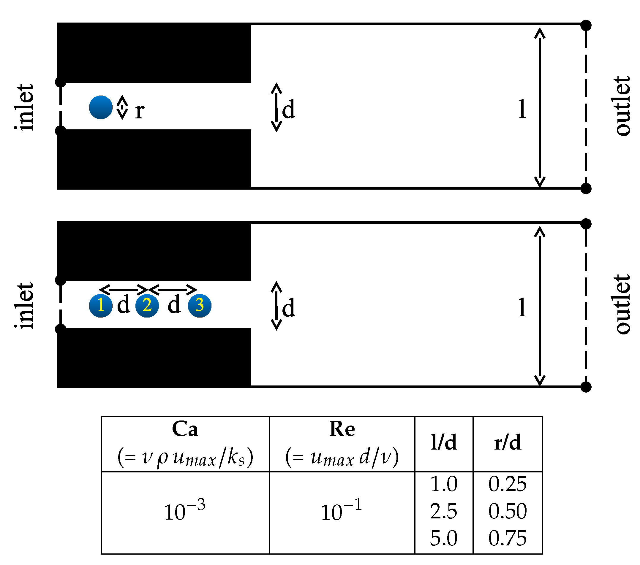
The simulations are performed for a two-dimensional domain as shown in Figure 1 and the fluid is considered to be water. The flow direction is left-to-right, the horizontal axis is denoted by the x-axis or co-axial direction, and the vertical axis is denoted by the y-axis or radial direction. The analysis is based on simulations either a single or three in-line spherical capsules, flowing from a channel of small diameter into that of a larger diameter, as shown in Figure 1. In subsequent discussion and presentation of results, we refer to the upstream direction as that closer to the inflow, and the downstream direction that closer to the outflow. One should, however, recognise that the capsule will be travelling faster than the bulk flow in the channel sections, since it is located furthest from the stationary walls. Consequently, in a moving reference frame following a capsule, its wake and disturbance it induces on the flow will in effect be in the upstream direction.
The computational domain is a rectangular channel by the height l and length with no-slip boundary conditions along y. The grid resolution is such that l is discretised with . The section is parametrised as a velocity inlet section with a parabolic inlet profile, while the outlet section is located at (see Figure 1) and is set as a convective condition [68]. The Reynolds number is fixed equal to 0.1 and is given by ; where is the maximum velocity for the plane Hagen–Poiseuille profile (parabolic profile) established in , d is the narrow channel diameter, and the kinematic viscosity of the fluid ( m/s). Note that represents the ratio of inertial to viscous forces and can also be interpreted as the ratio of viscous to convective time scales which act on the fluid. Here, the Reynolds number equals 0.1; consequently, viscous effects dominate, with viscous forces greater than inertial forces and the viscous time scale is smaller (hence acts faster, stabilising the flow) than the convective time scale. The capsules are initially at the rest, with no pre-stress applied, and of circular section with diameter r and stiffness modulated by the capillary number , where is the density of the fluid in which capsules are immersed ( kg/m) in and is the elastic constant used for the worm-like chain composing the membranes (see Equation (6)). represents the ratio of the viscous force to the elastic force consequently representing, within this definition, capsules slightly more rigid than in other studies [7,25]. Note that the typical stiffness for a red blood cell is Nm that would lead to Ca within this definition. To ensure the scheme stability, all the computations are performed with in the Lattice Boltzmann Method.
The present parametrisation deals with the deformation of a circular membrane in a rectangular two-dimensional channel injected into a reservoir. Given the narrow dimensions and axial symmetry of the problem and set-up, the results obtained are directly transferable to the analogous three-dimensional set-up. For a general case, the deformation and dynamics of initially spherical capsules in a three-dimensional circular capillary flowing into a reservoir will yield different quantitative results. However, the governing physics is unaltered and, while the mechanics in two or three dimensions is different, results from a two-dimensional investigation are transferable to a three-dimensional set-up and one can expect similar qualitative results and trends.
3. Results and Discussion
Numerical simulations for flow set-up outlined in Figure 1 were run for the following three cases: without capsules; with one capsule; with three capsules (numbered left-to-right). The available set-up combinations have resulted in a set of simulations, aimed at sampling the solution space in order to capture the physics of flow of capsules as they are injected into a reservoir. Videos of the simulations run are available online as Supplementary Files, organised by the capsule to channel ratio .
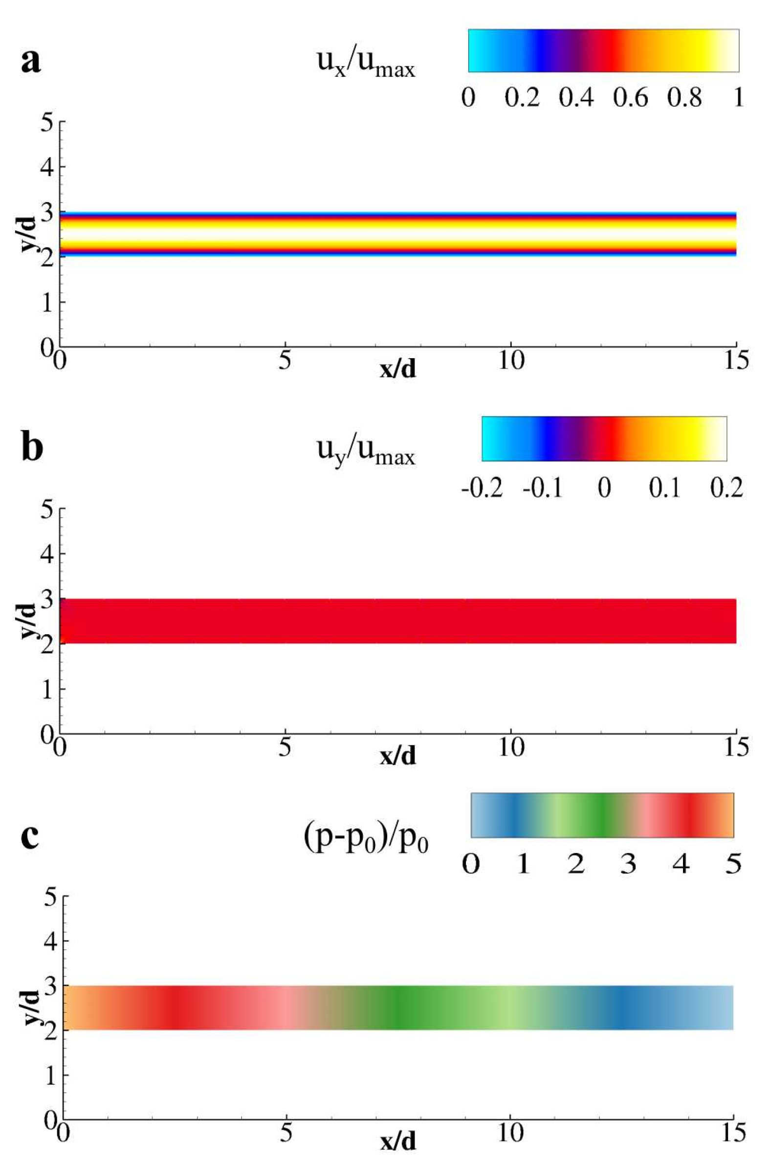
The solution for flow without any capsules are shown in Figure 2 and Figure A1 (in Appendix A), for purpose of comparison. As expected, we see the flow profile develop from the parabolic inflow profile to a flattened paraboloid profile on approaching the reservoir. The flow accelerates in the radial (vertical) direction and decelerates in the co-axial (horizontal) direction as it approaches the end of the smaller channel before discharging into the reservoir. The radial acceleration is effected by a pressure gradient which drives the flow to turn at the geometric discontinuity. The flow separates at the geometric discontinuity, reattaching onto the horizontal walls of the larger channel.
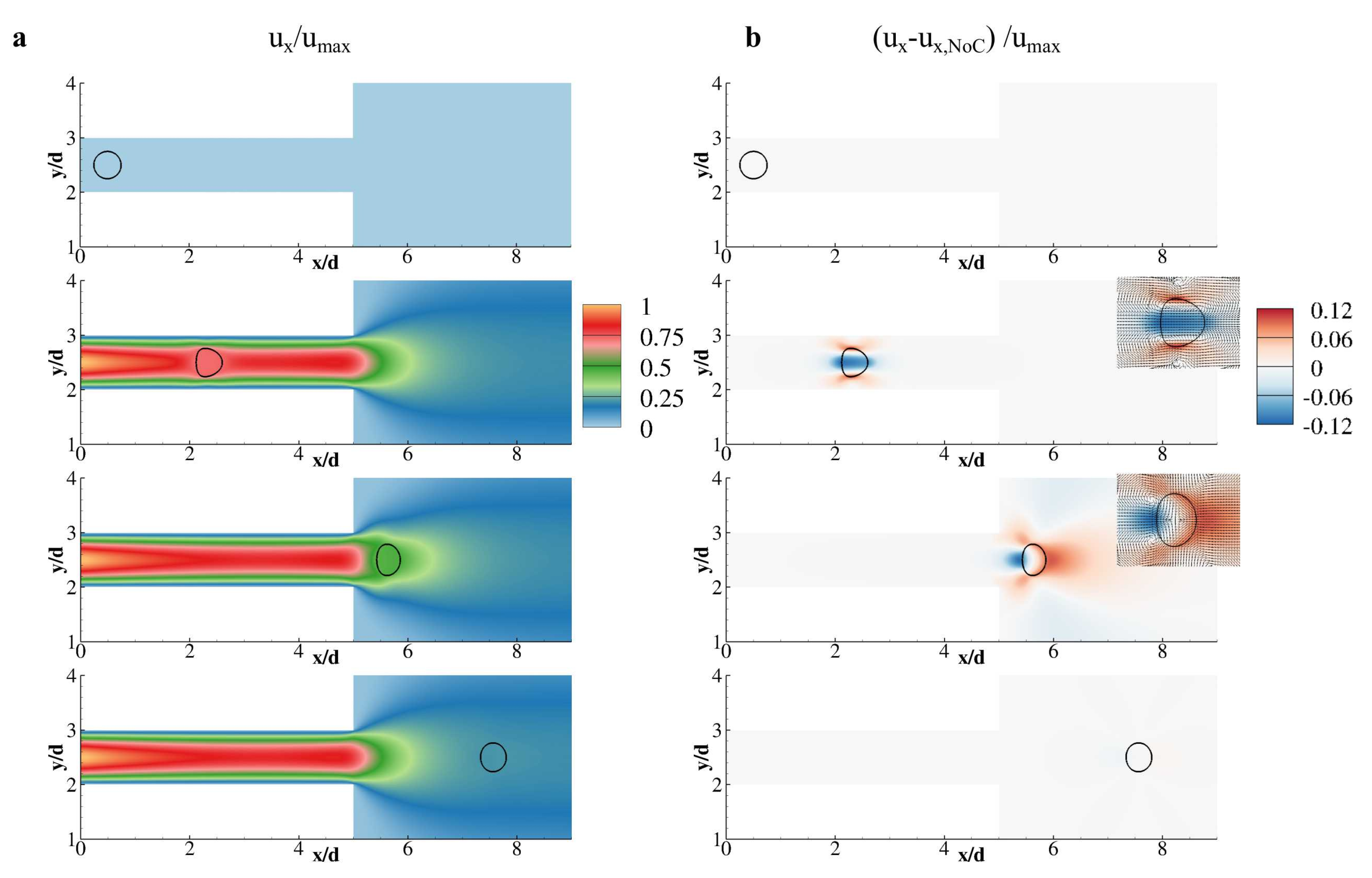
We now turn our attention to the ejection of a single capsule. While the results and discussion are transferable to the other set-up combinations, we present results for the geometry set-up and in Figure 3 as these favour presentation and discussion. In Figure 3, we present the (normalised) co-axial flow component, as well as the difference in flow velocity without capsules and with one capsule (coloured by co-axial velocity component). In the following presentation of results, this velocity difference is termed the relative velocity or relative flow field.
Let us first focus on results for time snapshot in Figure 3, when the capsule is located in the narrower channel. We observe that the presence of the capsule tends to create a more uniform velocity profile, by increasing the co-axial velocity near to the walls while decreasing it at the centre of the channel. The vector plot showing the relative velocity also shows that the presence of the flowing capsule results in flow around the capsule, from upstream to downstream. This is because the capsule in effect creates a resistance to the flow, causing it to flow more around it in comparison to the parabolic velocity profile. The relative flow field consequently appears as a vortex pair (or ring in three-dimensions) close to the wall, travelling with the capsule and aligned approximately at its maximum diameter. This vortex ring, identified in the relative flow field, induces a co-axial velocity which drives the capsule through the channel, and this can be seen by the higher velocity at the maximum diameter of the capsule. The wall shear stress is the tangential traction force that the flow exerts on the wall due to viscous effects, and we observe that, at the capsule’s maximum diameter, the co-axial velocity near the channel wall is the same as the parabolic flow, and hence the wall shear stress is effectively unaltered. However, slightly upstream and downstream of the capsule’s maximum diameter, we observe that the co-axial velocity near the wall is greater than for the parabolic profile, indicating a higher wall shear stress. This results in two locations (or rings in three-dimensions) of higher wall shear stress compared to the parabolic flow solution, travelling with the capsule and approximately aligned with the capsule’s leading and trailing edges. This is in contract to the results of the wall shear stress `footprint’ observed as red blood cells, which show a single higher band of wall shear stress as the deformable cells are in proximity to the walls [31,36,37].
We now turn our attention to results for time snapshot in Figure 3, when the capsule has been ejected into the reservoir. We observe that, for this instance, the mean velocity of the capsule is the same as a solution when no capsule is present, while, in comparison, the flow is moving faster in front of the capsule and slower behind. We also observe that the relative flow field presents a vortex ring at the trailing side of the capsule, travelling with the capsule. This vortex ring is counter-rotating to the vortex ring observed in the narrower channel section, and is set up by the geometric discontinuity. The direction of rotation of this vortex ring induces a velocity that promotes the flow to turn around the geometric discontinuity and results in a smaller flow separation. The induced velocity of this vortex ring also acts to decelerate the capsule co-axial motion as it ejects into the reservoir.
Finally, we note that, for time snapshot , the flow of a single capsule in a large channel or reservoir has no marked influence on the flow field as compared to the above discussed time snapshots 5 and 10.
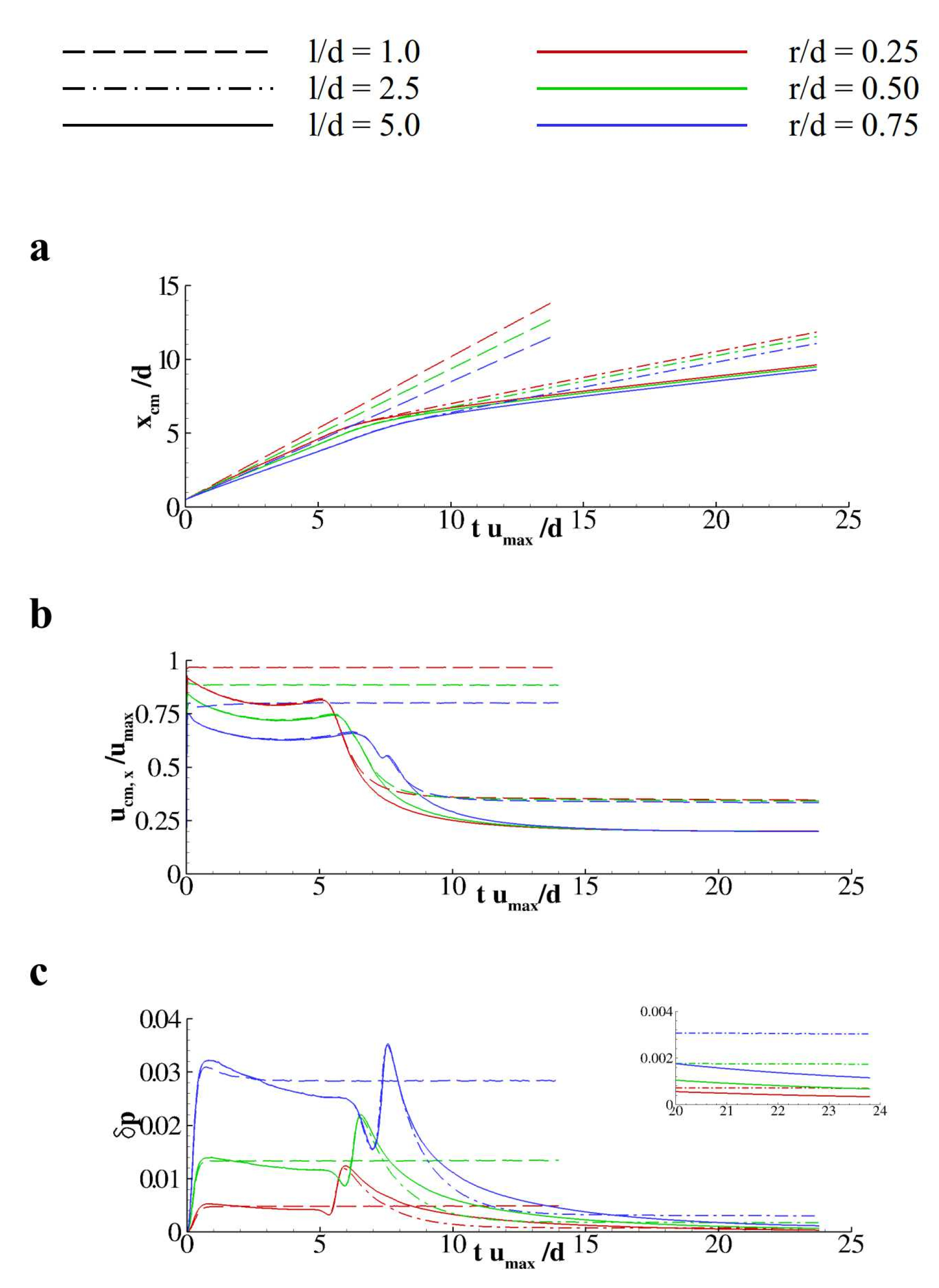
Similar flow fields and relative flow fields were observed in the other set-up combinations. We turn our attention therefore to the motion of the capsule and its change in perimeter length, presented in Figure 4, and investigate the effects of the geometric variations based on the ratio and . Overall, the trends appear linear as one varies the geometric ratios and ; however, there are some small deviations that are worth highlighting and discussing.
For comparison purposes in this figure, the case for (straight channel without discontinuity) is also plotted. We observe that the capsule velocity and perimeter length change are constant (after rapid adjustment from the zero velocity initial conditions of the simulations); however, there are variations based on the ratio. At larger values of , the capsule forms a larger blockage in the channel, and we observe that a more blunt velocity profile is caused by the capsule compared to the capsule. The greater perimeter length change is also observed for the capsule, since there are larger shear rates in proximity with the channel wall aligned to the capsule’s largest diameter as it flows. This was observed in Figure 3 from the relative flow field.
We now focus on the channel geometry set-up with 2.5 and 5.0 within Figure 4. We observe that the traces of normalised co-axial position for capsules with 0.25 and 0.50 lie closer than for capsule . The lag is seen to appear at the moment when the capsule is injected into the reservoir, with . We observe that the traces of normalised co-axial velocity are indistinguishable while the capsule lies within the narrower channel, and parallel based on their value. The capsule velocity then transits to the similar values once the capsule enters the reservoir occurs rapidly, now based on the value of , while the ratio has little effect. For and , we observe that there is a secondary peak in the velocity at . We observe that the perimeter length change is relatively constant as the capsule travels along the narrower channel but decreases and then increases sharply as the capsule is ejected into the reservoir. The decrease in perimeter length is due to the capsule leading edge slowing down as it reaches the reservoir, resulting in a decrease in membrane stress. The subsequent increase in perimeter length occurs as the capsule completes its transition into the reservoir, during which the anterior portion of the capsule is already in the reservoir and has a low velocity; however, the posterior portion of the capsule still has a larger velocity, causing the capsule to flatten (stretching radially). Once in the reservoir, the capsule membrane relaxes and tends to assume an undeformed shape. The change in perimeter length is larger in the narrower channel due to higher shear rates, more so with an increasing ratio, which was also observed from the relative flow field shown in Figure 3. For and , we observe that the sudden decrease and subsequent increase in perimeter lengths were in proportions higher than other cases.
Focusing on the case with and , we summarise that we observed a different behaviour as the capsule was ejected into the reservoir, compared to the other simulations. This led to a lag in its co-axial position, a second peak in the co-axial velocity and more pronounced change in the perimeter length. The reasons for these phenomena are principally due to the size of the capsule, which owing to the membrane have the effect of locally constraining the flow to be more uniform (hence a homogeneous velocity field). Capsule deformability and the elastic forces are also important, without which we would not obtain the second velocity peak, for example.
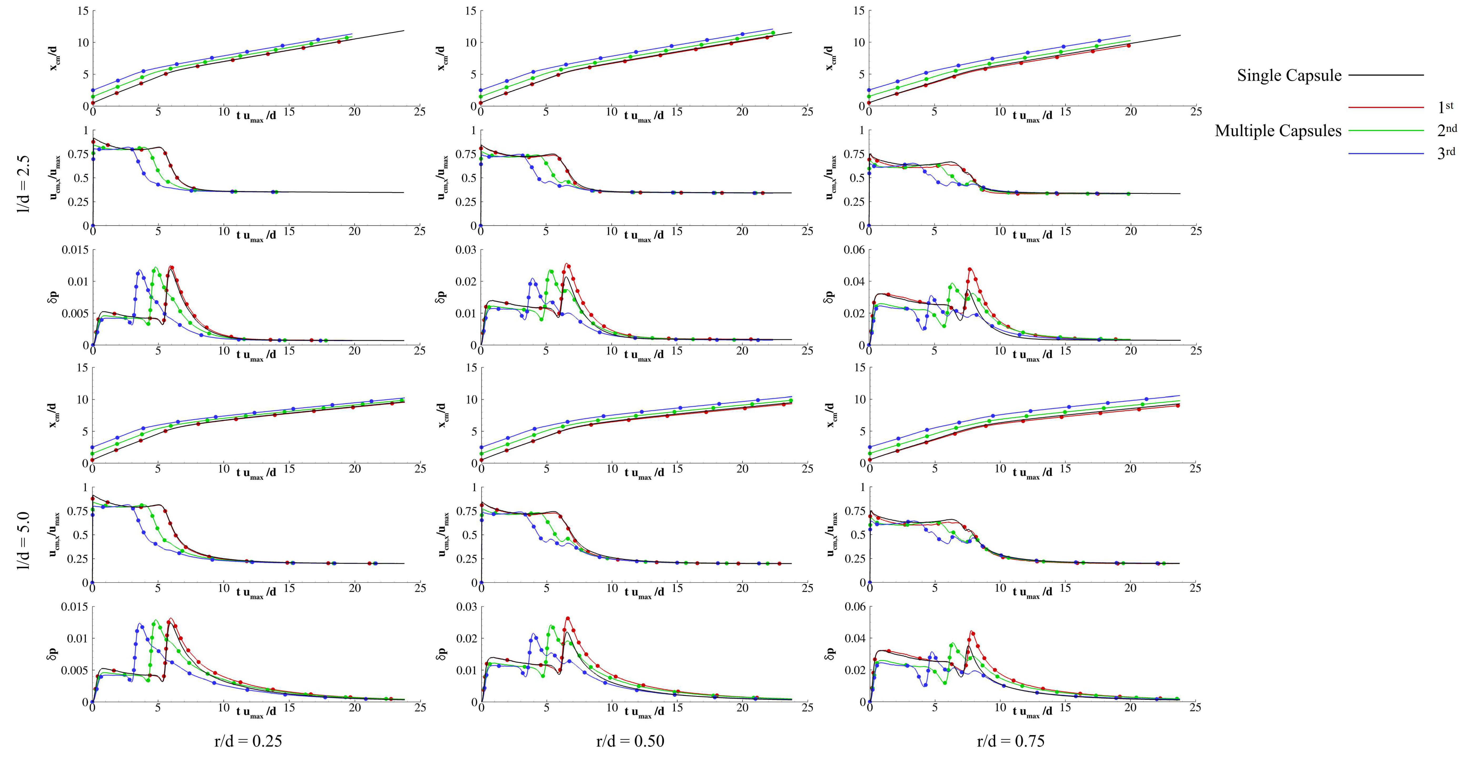
We now turn our attention to the results for three capsules flowing in the channel and ejecting into the reservoirs. The flow field and relative velocity for the geometry set-up and with three capsules are presented in Figure 5. In comparison to the flow of the single capsule (see Figure 3), we see that, within the narrow channel, the disturbance in the flow field extends to influence both upstream and downstream capsules, due to their relative proximity. Specifically, the capsules effect a blunter velocity profile with respect to the parabolic profile (obtained without capsules). This phenomenon is often described by a shear-thinning non-Newtonian model for the viscosity. At time , when the capsules are entirely in the reservoir, the leading capsules (capsules 2 and 3) are travelling faster than is the case without capsules, while the left-most capsule (capsule 1) is travelling slower. This is again due to the capsule acting to locally constrain the flow to be more uniform, and in this case extending the apparent jet formed by the flow ejecting from the narrower channel into the reservoir. At this time instance, we also note that a vortex ring is formed at the trailing section of capsule 1 only, further highlighting that the flow disturbances between the three capsules result in a local homogenisation of the velocity field, and the capsules therefore tend to act as a single larger object.
In Figure 6, the properties of the single capsule (also shown in Figure 4) and of the multiple particles are plotted as function of normalised time. We notice that the effect of the relative reservoir diameter, , does not play a noticeable influence beyond a given size. Additionally, we observe a greater effect of the multiple capsules when they are larger, and therefore focus our presentation of results for the set-up and . The discussion is amenable to the other set-up cases, and differences are presented. In general, for the smaller capsules with 0.50 and 0.25 the same phenomena are present as for the larger capsules, but to a lesser extent. Indeed, for the smallest capsules , the effect of the multiple cells is almost imperceivable. The reason for this is a reduced inter-capsule interaction, due to the relatively large capsule separation distance and the small capsule size that will not significantly affect the flow field.
In Figure 6, observing the traces for set-up and , we first note that the capsules exhibit oscillating velocities and change in perimeter, more marked for capsule 3 and least for capsule 1. These oscillations are related to the ejection of capsules into the reservoir and we see, for example, that, as capsule 1 enters the reservoir, it induces an oscillation in both capsules 2 and 3. This chain effect is due to the capsules effectively constraining the fluid, and locally homogenising the velocity field. The apparent viscosity is locally higher, and the capsules, due to their close proximity, effectively act as a single larger body. Another phenomenon of particular interest is that capsule 3 tends to move overall faster, and, from the trace, we see that it is farther from capsules 1 and 2 towards later times. In order to explain this, we turn to Figure 5. We observe that the relative velocity is greatest ahead of capsule 3 when the capsules are in the reservoir (at time ) and the flow is in the narrower channel a short distance ahead of capsule 3 is undisturbed and parabolic. Since capsule 3 is at the leading edge of the capsules, it is not affected by the wake and will be able to travel faster. This phenomenon of capsule spacing rearrangement was also observed in [16], though in very different geometries. Finally, we note that the perimeter stretching is greatest overall for capsule 1, due to its location in the end of the capsule train, inducing a more marked wake and consequently higher shear rate (velocity gradients) in the fluid and higher stresses in its membrane. In fact, we observe that the change in perimeter length is comparable to the set-up of the single capsule, since it has a similar wake flow field.
4. Conclusions
In this work, we investigate the dynamics of capsule ejection from a narrow channel into a reservoir, across a geometric discontinuity. We observe that inter-capsule interaction (due to the wakes of their motion) and the constraining of the fluid within the membranes are an important mechanism that affects the local apparent viscosity since the stress field must be continuous in the domain.
In order to span a meaningful parameter space, a combination of different configurations was investigated. The capsules were varied to have different sizes, namely 0.25, 0.50 and 0.75, where r is the capsule diameter and d is the narrow channel diameter. Three configurations of channel geometries were investigated, namely 1.0, 2.5 and 5.0, where l is the diameter of the reservoir. Additionally, three different configurations: no capsule, a single capsule, and three in-line capsules, were simulated and investigated. The Capillary number and Reynolds numbers were chosen to be and .
The simulations were investigated by observing the relative flow field that is the flow field resulting from capsule flow as compared to the no capsule solutions. This has proved to be an effective means of identifying where the flow field has altered, and, consequently, to identify the fluid mechanics phenomena causing the changes observed. Additionally, the trajectories, velocities and perimeters of the capsules were tracked during the simulations.
Overall, we have seen that the reservoir diameter has a negligible effect beyond a threshold, and, in the resent investigation, similar results were obtained for and . The effect of capsule size was seen to be have a greater effect, with unsurprisingly resulting in the greatest deviation from a flow field with no capsule, however capsules with size were also seen to affect the flow field.
Capsule membranes constrain the flow internally, and since the stress field must be continuous across the capsule membrane, the effect is to locally homogenise (i.e., create greater uniformity) the velocity field. This can be seen as a local increase in apparent viscosity. When multiple capsules were investigated, the inter-capsule interaction caused the capsules to effectively act as a single larger body. This resulted in an increased apparent viscosity spanning the region of the capsules. This effect was clearly observed as the capsules flow in the narrow channel, for which the apparent viscosity resembled that of a shear-thinning non-Newtonian rheological model. An effect of the local increased viscosity is also the cause that the leading capsule tends to move faster than the other two trailing capsules.
The effect of the multiple capsules is to reduce the perimeter change, due to their wakes and inter-capsule interaction which reduces the shear rate (i.e., velocity gradients) of the fluid integrated over the capsule surface. This then leads to a decrease in overall strain for the capsule membrane. The capsule at the trailing edge however is not shielded and its wake promotes a vortex ring in the relative velocity field, and its perimeter change is the same as that of a single capsule flow.
Lastly, we highlight that, while the two-dimensional results reported here are representative of the analogous three-dimensional problem, due to the symmetry and regimes (based on capillary and Reynolds numbers) of the set-up, this is generally not the case. Indeed, in complex systems, such as a general set-up where deformable capsules are injected into a reservoir, not only are the mechanics of the jet collapse different between two and three dimensions, importantly also the specific stresses involved in the fluid–structure interactions will differ. This noted, two-dimensional simulations can still provide fruitful information on the regulating biophysical mechanisms without the inconvenience of the computationally intense three-dimensional simulations. The extension of the current physical problem to three-dimensional modelling is certainly of interest and will be the object of future investigations.
Supplementary Materials
The following are available online at https://www.mdpi.com/2311-5521/4/3/122/s1. Video set rd025: results for the channel with ratio . Video set rd050: results for the channel with ratio . Video set rd075: results for the channel with ratio .
Author Contributions
The authors equally contributed to this research.
Funding
This research received no external funding.
Acknowledgments
The authors acknowledge Giuseppe Pascazio and Marco Donato de Tullio for providing CPU hours.
Conflicts of Interest
The authors declare no conflict of interest.
Appendix A
Figure A1.
Flow patterns in the micro-channel. (a) contour of the longitudinal component of the velocity field; (b) contour of the vertical component of the velocity field; (c) relative pressure distribution in the computational flow field ( is the outlet section pressure).
Figure A1.
Flow patterns in the micro-channel. (a) contour of the longitudinal component of the velocity field; (b) contour of the vertical component of the velocity field; (c) relative pressure distribution in the computational flow field ( is the outlet section pressure).

Figure A2.
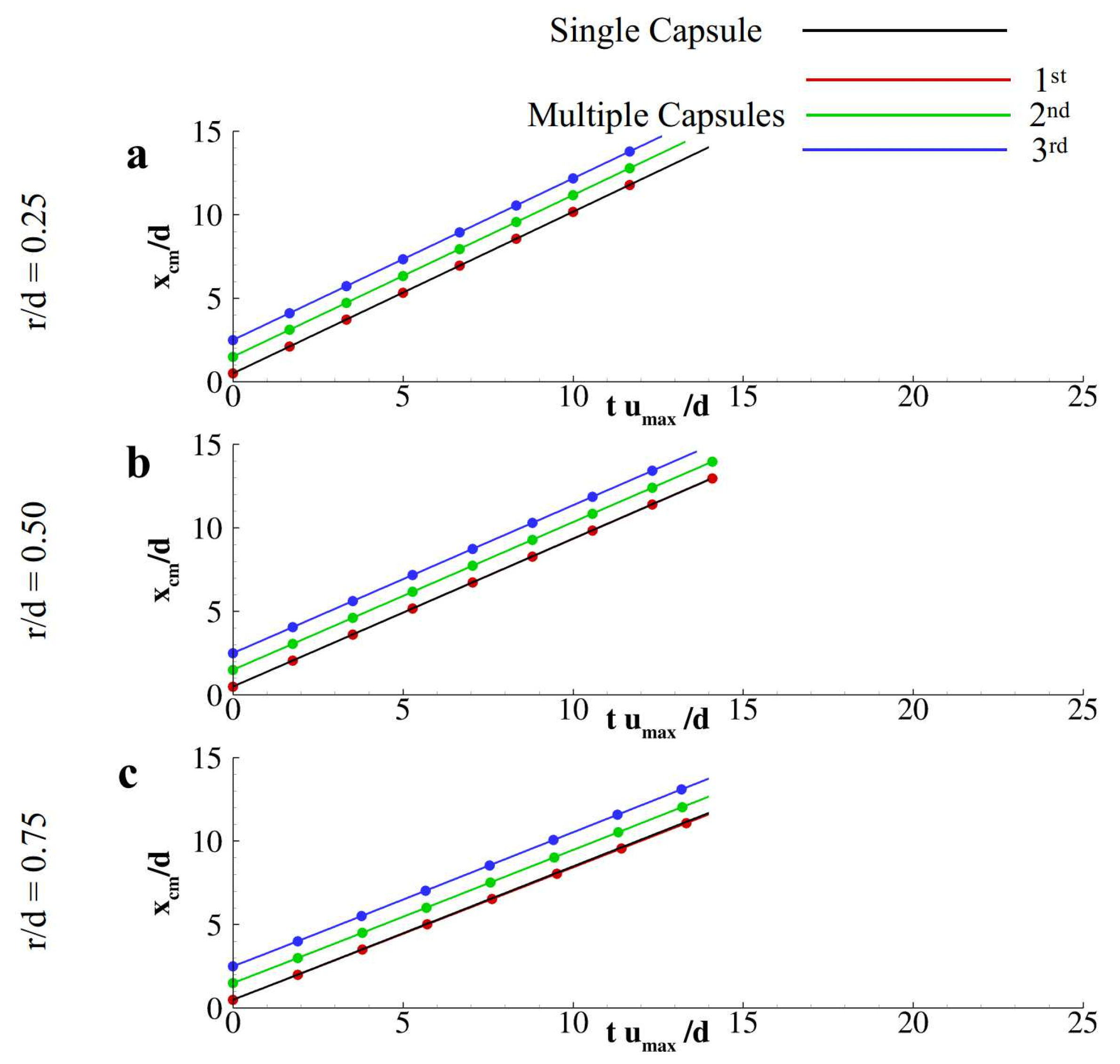
Transport of three aligned capsules () in the micro-channel. Distribution of the x-coordinate of the capsule centre of mass over time for (a); (b); and (c).
Figure A2.
Transport of three aligned capsules () in the micro-channel. Distribution of the x-coordinate of the capsule centre of mass over time for (a); (b); and (c).

References
- Robertson, A.M.; Sequeira, A.; Kameneva, M.V. Hemorheology. In Hemodynamical Flows; Springer: Berlin, Germany, 2008; pp. 63–120. [Google Scholar]
- Robertson, A.M.; Sequeira, A.; Owens, R.G. Rheological models for blood. In Cardiovascular Mathematics; Springer: Berlin, Germany, 2009; pp. 211–241. [Google Scholar]
- Goldsmith, H. Red cell motions and wall interactions in tube flow. Fed. Proc. 1971, 30, 1578–1590. [Google Scholar] [PubMed]
- Pozrikidis, C. Finite deformation of liquid capsules enclosed by elastic membranes in simple shear flow. J. Fluid Mech. 1995, 297, 123–152. [Google Scholar] [CrossRef]
- Matsunaga, D.; Imai, Y.; Yamaguchi, T.; Ishikawa, T. Rheology of a dense suspension of spherical capsules under simple shear flow. J. Fluid Mech. 2016, 786, 110–127. [Google Scholar] [CrossRef]
- Tsubota, K.I.; Wada, S. Effect of the natural state of an elastic cellular membrane on tank-treading and tumbling motions of a single red blood cell. Phys. Rev. E 2010, 81, 011910. [Google Scholar] [CrossRef] [PubMed]
- Nix, S.; Imai, Y.; Matsunaga, D.; Yamaguchi, T.; Ishikawa, T. Lateral migration of a spherical capsule near a plane wall in Stokes flow. Phys. Rev. E 2014, 90, 043009. [Google Scholar] [CrossRef]
- Omori, T.; Imai, Y.; Yamaguchi, T.; Ishikawa, T. Reorientation of a nonspherical capsule in creeping shear flow. Phys. Rev. Lett. 2012, 108, 138102. [Google Scholar] [CrossRef]
- Matsunaga, D.; Imai, Y.; Yamaguchi, T.; Ishikawa, T. Deformation of a spherical capsule under oscillating shear flow. J. Fluid Mech. 2015, 762, 288–301. [Google Scholar] [CrossRef]
- Fedosov, D.A.; Lei, H.; Caswell, B.; Suresh, S.; Karniadakis, G.E. Multiscale modeling of red blood cell mechanics and blood flow in malaria. PLoS Comput. Biol. 2011, 7, e1002270. [Google Scholar] [CrossRef]
- Fedosov, D.A.; Noguchi, H.; Gompper, G. Multiscale modeling of blood flow: From single cells to blood rheology. Biomech. Model. Mechanobiol. 2014, 13, 239–258. [Google Scholar] [CrossRef]
- Faivre, M.; Abkarian, M.; Bickraj, K.; Stone, H.A. Geometrical focusing of cells in a microfluidic device: An approach to separate blood plasma. Biorheology 2006, 43, 147–159. [Google Scholar]
- Yaginuma, T.; Oliveira, M.S.; Lima, R.; Ishikawa, T.; Yamaguchi, T. Human red blood cell behavior under homogeneous extensional flow in a hyperbolic-shaped microchannel. Biomicrofluidics 2013, 7, 054110. [Google Scholar] [CrossRef] [PubMed] [Green Version]
- Faustino, V.; Catarino, S.O.; Lima, R.; Minas, G. Biomedical microfluidic devices by using low-cost fabrication techniques: A review. J. Biomech. 2016, 49, 2280–2292. [Google Scholar] [CrossRef] [PubMed] [Green Version]
- Rodrigues, R.O.; Lopes, R.; Pinho, D.; Pereira, A.I.; Garcia, V.; Gassmann, S.; Sousa, P.C.; Lima, R. In vitro blood flow and cell-free layer in hyperbolic microchannels: Visualizations and measurements. BioChip J. 2016, 10, 9–15. [Google Scholar] [CrossRef]
- Di Carlo, D.; Irimia, D.; Tompkins, R.G.; Toner, M. Continuous inertial focusing, ordering, and separation of particles in microchannels. Proc. Natl. Acad. Sci. USA 2007, 104, 18892–18897. [Google Scholar] [CrossRef] [PubMed] [Green Version]
- Hsu, C.H.; Di Carlo, D.; Chen, C.; Irimia, D.; Toner, M. Microvortex for focusing, guiding and sorting of particles. Lab Chip 2008, 8, 2128–2134. [Google Scholar] [CrossRef] [PubMed] [Green Version]
- Tanaka, T.; Ishikawa, T.; Numayama-Tsuruta, K.; Imai, Y.; Ueno, H.; Matsuki, N.; Yamaguchi, T. Separation of cancer cells from a red blood cell suspension using inertial force. Lab Chip 2012, 12, 4336–4343. [Google Scholar] [CrossRef] [PubMed]
- Omori, T.; Imai, Y.; Kikuchi, K.; Ishikawa, T.; Yamaguchi, T. Hemodynamics in the microcirculation and in microfluidics. Ann. Biomed. Eng. 2015, 43, 238–257. [Google Scholar] [CrossRef] [PubMed]
- Pinho, D.; Yaginuma, T.; Lima, R. A microfluidic device for partial cell separation and deformability assessment. BioChip J. 2013, 7, 367–374. [Google Scholar] [CrossRef] [Green Version]
- Bento, D.; Rodrigues, R.; Faustino, V.; Pinho, D.; Fernandes, C.; Pereira, A.; Garcia, V.; Miranda, J.; Lima, R. Deformation of red blood cells, air bubbles, and droplets in microfluidic devices: Flow visualizations and measurements. Micromachines 2018, 9, 151. [Google Scholar] [CrossRef]
- Yoon, D.H.; Ha, J.B.; Bahk, Y.K.; Arakawa, T.; Shoji, S.; Go, J.S. Size-selective separation of micro beads by utilizing secondary flow in a curved rectangular microchannel. Lab Chip 2009, 9, 87–90. [Google Scholar] [CrossRef]
- Martel, J.M.; Toner, M. Inertial focusing dynamics in spiral microchannels. Phys. Fluids 2012, 24, 032001. [Google Scholar] [CrossRef] [PubMed] [Green Version]
- Losserand, S.; Coupier, G.; Podgorski, T. Migration velocity of red blood cells in microchannels. Microvasc. Res. 2019, 124, 30–36. [Google Scholar] [CrossRef] [PubMed] [Green Version]
- Omori, T.; Ishikawa, T.; Barthès-Biesel, D.; Salsac, A.V.; Imai, Y.; Yamaguchi, T. Tension of red blood cell membrane in simple shear flow. Phys. Rev. E 2012, 86, 056321. [Google Scholar] [CrossRef] [PubMed] [Green Version]
- Sudarsan, A.P.; Ugaz, V.M. Multivortex micromixing. Proc. Natl. Acad. Sci. USA 2006, 103, 7228–7233. [Google Scholar] [CrossRef] [PubMed] [Green Version]
- Coclite, A.; Pascazio, G.; de Tullio, M. D.; Decuzzi, P. Predicting the vascular adhesion of deformable drug carriers in narrow capillaries traversed by blood cells. J. Fluids Struct. 2018, 82, 638–650. [Google Scholar] [CrossRef]
- Coclite, A.; Mollica, H.; Ranaldo, S.; Pascazio, G.; de Tullio, M.D.; Decuzzi, P. Predicting different adhesive regimens of circulating particles at blood capillary walls. Microfluid. Nanofluid. 2017, 21, 168. [Google Scholar] [CrossRef] [Green Version]
- Mollica, H.; Coclite, A.; Miali, M.E.; Pereira, R.C.; Paleari, L.; Manneschi, C.; DeCensi, A.; Decuzzi, P. Deciphering the relative contribution of vascular inflammation and blood rheology in metastatic spreading. Biomicrofluidics 2018. [Google Scholar] [CrossRef]
- Decuzzi, P.; Godin, B.; Tanaka, T.; Lee, S.Y.; Chiappini, C.; Liu, X.; Ferrari, M. Size and shape effects in the biodistribution of intravascularly injected particles. J. Control. Release 2010, 141, 320–327. [Google Scholar] [CrossRef]
- Gambaruto, A.M. Flow structures and red blood cell dynamics in arteriole of dilated or constricted cross section. J. Biomech. 2016, 49, 2229–2240. [Google Scholar] [CrossRef] [Green Version]
- Gong, X.; Sugiyama, K.; Takagi, S.; Matsumoto, Y. The deformation behavior of multiple red blood cells in a capillary vessel. J. Biomech. Eng. 2009, 131, 074504. [Google Scholar] [CrossRef]
- Bessonov, N.; Babushkina, E.; Golovashchenko, S.; Tosenberger, A.; Ataullakhanov, F.; Panteleev, M.; Tokarev, A.; Volpert, V. Numerical modelling of cell distribution in blood flow. Math. Model. Nat. Phenom. 2014, 9, 69–84. [Google Scholar] [CrossRef]
- Vahidkhah, K.; Balogh, P.; Bagchi, P. Flow of red blood cells in stenosed microvessels. Sci. Rep. 2016, 6, 28194. [Google Scholar] [CrossRef] [PubMed]
- Sun, C.; Munn, L.L. Influence of erythrocyte aggregation on leukocyte margination in postcapillary expansions: A lattice Boltzmann analysis. Phys. A Stat. Mech. Its Appl. 2006, 362, 191–196. [Google Scholar] [CrossRef]
- Xiong, W.; Zhang, J. Shear stress variation induced by red blood cell motion in microvessel. Ann. Biomed. Eng. 2010, 38, 2649–2659. [Google Scholar] [CrossRef] [PubMed]
- Freund, J.B.; Vermot, J. The wall-stress footprint of blood cells flowing in microvessels. Biophys. J. 2014, 106, 752–762. [Google Scholar] [CrossRef] [PubMed]
- Takeishi, N.; Imai, Y.; Ishida, S.; Omori, T.; Kamm, R.D.; Ishikawa, T. Cell adhesion during bullet motion in capillaries. Am. J. Physiol. Heart Circ. Physiol. 2016, 311, H395–H403. [Google Scholar] [CrossRef] [Green Version]
- Takeishi, N.; Imai, Y.; Nakaaki, K.; Yamaguchi, T.; Ishikawa, T. Leukocyte margination at arteriole shear rate. Physiol. Rep. 2014, 2. [Google Scholar] [CrossRef]
- Muller, K.; Fedosov, D.; Gompper, G. Margination of micro- and nano-particles in blood flow and its effect on drug delivery. Sci. Rep. 2014, 4. [Google Scholar] [CrossRef]
- Takeishi, N.; Imai, Y. Capture of microparticles by bolus flow of red blood cells in capillaries. Sci. Rep. 2017, 7, 5381. [Google Scholar] [CrossRef]
- Gambaruto, A.M. Computational haemodynamics of small vessels using the moving particle semi-implicit (MPS) method. J. Comput. Phys. 2015, 302, 68–96. [Google Scholar] [CrossRef]
- Alizadehrad, D.; Imai, Y.; Nakaaki, K.; Ishikawa, T.; Yamaguchi, T. Quantification of red blood cell deformation at high-hematocrit blood flow in microvessels. J. Biomech. 2012, 45, 2684–2689. [Google Scholar] [CrossRef] [PubMed]
- Tanaka, N.; Takano, T. Microscopic-scale simulation of blood flow using SPH method. Int. J. Comput. Methods 2005, 2, 555–568. [Google Scholar] [CrossRef]
- Noguchi, H.; Gompper, G. Swinging and tumbling of fluid vesicles in shear flow. Phys. Rev. Lett. 2007, 98, 128103. [Google Scholar] [CrossRef] [PubMed]
- Bakhshian, S.; Sahimi, M. Computer simulation of the effect of deformation on the morphology and flow properties of porous media. Phys. Rev. E 2016, 94, 042903. [Google Scholar] [CrossRef] [PubMed] [Green Version]
- Bakhshian, S.; Hosseini, S.A.; Shokri, N. Pore-scale characteristics of multiphase flow in heterogeneous porous media using the lattice Boltzmann method. Sci. Rep. 2019, 9, 3377. [Google Scholar] [CrossRef] [PubMed]
- Bhatnagar, P.L.; Gross, E.P.; Krook, M. A Model for Collision Processes in Gases. I. Small Amplitude Processes in Charged and Neutral One-Component Systems. Phys. Rev. 1954, 94, 511–525. [Google Scholar] [CrossRef]
- Qian, Y.H.; d’Humières, D.; Lallemand, P. Lattice BGK models for Navier–Stokes equation. EPL Europhys. Lett. 1992, 17, 479. [Google Scholar] [CrossRef]
- Shan, X.; Yuan, X.F.; Chen, H. Kinetic theory representation of hydrodynamics: A way beyond the Navier–Stokes equation. J. Fluid Mech. 2006, 550, 413–441. [Google Scholar] [CrossRef]
- Pozrikidis, C. Effect of membrane bending stiffness on the deformation of capsules in simple shear flow. J. Fluid Mech. 2001, 440, 269–291. [Google Scholar] [CrossRef]
- Skalak, R.; Tozeren, A.; Zarda, R.; Chien, S. Strain energy function of red blood cell membranes. Biophys. J. 1973, 13, 245–264. [Google Scholar] [CrossRef]
- Krüger, H. Computer Simulation Study of Collective Phenomena in Dense Suspensions of Red Blood Cells under Shear; Springer Science & Business Media: Berlin, Germany, 2012. [Google Scholar]
- Dao, M.; Li, J.; Suresh, S. Molecularly based analysis of deformation of spectrin network and human erythrocyte. Mater. Sci. Eng. C 2006, 26, 1232–1244. [Google Scholar] [CrossRef]
- Nakamura, M.; Bessho, S.; Wada, S. Spring-network-based model of a red blood cell for simulating mesoscopic blood flow. Int. J. Numer. Methods Biomed. Eng. 2013, 29, 114–128. [Google Scholar] [CrossRef] [PubMed]
- Ye, S.S.; Ng, Y.C.; Tan, J.; Leo, H.L.; Kim, S. Two-dimensional strain-hardening membrane model for large deformation behavior of multiple red blood cells in high shear conditions. Theor. Biol. Med Model. 2014, 11, 19. [Google Scholar] [CrossRef] [PubMed]
- Guo, Z.; Zheng, C.; Shi, B. Force imbalance in lattice Boltzmann equation for two-phase flows. Phys. Rev. E 2011, 83, 036707. [Google Scholar] [CrossRef] [PubMed]
- De Rosis, A.; Ubertini, S.; Ubertini, F. A Comparison Between the Interpolated Bounce-Back Scheme and the Immersed Boundary Method to Treat Solid Boundary Conditions for Laminar Flows in the Lattice Boltzmann Framework. J. Sci. Comput. 2014, 61, 477–489. [Google Scholar] [CrossRef]
- Ubertini, A.D.R.S.U.F. A partitioned approach for two-dimensional fluid-structure interaction problems by a coupled lattice Boltzmann-finite element method with immersed boundary. J. Fluids Struct. 2014, 45, 202–215. [Google Scholar] [CrossRef]
- Suzuki, K.; Minami, K.; Inamuro, T. Lift and thrust generation by a butterfly-like flapping wing-body model: Immersed boundary-lattice Boltzmann simulations. J. Fluid Mech. 2015, 767, 659–695. [Google Scholar] [CrossRef]
- Wang, Y.; Shu, C.; Teo, C. J.; Wu, J. An immersed boundary-lattice Boltzmann flux solver and its applications to fluid-structure interaction problems. J. Fluids Struct. 2015, 54, 440–465. [Google Scholar] [CrossRef]
- Zou, Q.; He, X. On pressure and velocity boundary conditions for the lattice Boltzmann BGK model. Phys. Fluids 1997, 9, 1591–1598. [Google Scholar] [CrossRef] [Green Version]
- Coclite, A.; de Tullio, M.D.; Pascazio, G.; Decuzzi, P. A combined Lattice Boltzmann and Immersed boundary approach for predicting the vascular transport of differently shaped particles. Comput. Fluids 2016, 136, 260–271. [Google Scholar] [CrossRef] [Green Version]
- Coclite, A.; Ranaldo, S.; de Tullio, M.; Decuzzi, P.; Pascazio, G. Kinematic and Dynamic Forcing Strategies for Predicting the Transport of Inertial Capsules Via A Combined Lattice Boltzmann Immersed Boundary Method. Comput. Fluids 2019, 180, 41–53. [Google Scholar] [CrossRef]
- Balaras, M.V.E. A moving-least-squares reconstruction for embedded-boundary formulations. J. Comput. Phys. 2009, 6617–6628. [Google Scholar] [CrossRef]
- Favier, J.; Revell, A.; Pinelli, A. A Lattice Boltzmann-Immersed Boundary method to simulate the fluid interaction with moving and slender flexible objects. J. Comput. Phys. 2014, 261, 145–161. [Google Scholar] [CrossRef]
- de Tullio, M.D.; Pascazio, G. A moving-least-squares immersed boundary method for simulating the fluid–structure interaction of elastic bodies with arbitrary thickness. J. Comput. Phys. 2016, 325, 201–225. [Google Scholar] [CrossRef]
- Yang, Z. Lattice Boltzmann outflow treatments: Convective conditions and others. Comput. Math. Appl. 2013, 65, 160–171. [Google Scholar] [CrossRef]
Figure 1.
Schematic of the physical problem. (Top) sketch of the computational domain with characteristics dimensions and lengths, as well as boundary conditions; (Bottom) non-dimensional groups used in the computations: the capillary number regulating the mechanical stiffness of the membranes, ; the Reynolds number regulating the flow velocity, ; the ratio between channel diameter and reservoir height, , and the ratio between particle diameter and reservoir height, .

Figure 2.
Flow patterns for different width of the reservoir. (a) contour of the longitudinal component of the velocity field for 2.5 (left) and 5.0 (right); (b) contour of the vertical component of the velocity field for 2.5 (left) and 5.0 (right); (c) relative pressure distribution in the computational flow field ( is the outlet section pressure). Data for 1.0 are shown in Appendix A.

Figure 3.
Flow patterns during the transport of a single capsule in the micro-channel. (a) contour of the longitudinal velocity field for 5.0 and 0.50 taken at four different time steps, namely 0, 5, 10, and 20; (b) contour plot of difference between the longitudinal velocity with () and without () the capsule immersed in at four different time steps, namely 0, 5, 10, and 20.

Figure 4.
Injection of a capsule in a reservoir. (a) distribution of the x-coordinate of the capsule centre of mass over time; (b) distribution of the x-velocity of the capsule centre of mass over time; (c) distribution of the capsule stretching computed as the relative difference between the current, p, and the initial, , perimeter of the capsule ().

Figure 5.
Flow patterns during the transport of three aligned capsules in the micro-channel. (a) contour of the longitudinal velocity field for 5.0 and 0.50 taken at four different time steps, namely 0, 5, 10, and 20; (b) contour plot of difference between the longitudinal velocity with () and without () the capsules immersed in at four different time steps, namely 0, 5, 10, and 20.

Figure 6.
Transport of three aligned capsules in the micro-channel, for capsule diameter to channel ratio: left column (); middle column (); right column (). (a) distribution of the x-coordinate of the capsule centre of mass over time for (top) and (bottom); (b) distribution of the x-velocity of the capsule centre of mass over time for (top) and (bottom); (c) distribution of the capsule stretching computed as the relative difference between the current, p, and the initial, , perimeter of the capsule () for (top) and (bottom).

© 2019 by the authors. Licensee MDPI, Basel, Switzerland. This article is an open access article distributed under the terms and conditions of the Creative Commons Attribution (CC BY) license (http://creativecommons.org/licenses/by/4.0/).
Share and Cite
MDPI and ACS Style
Coclite, A.; Gambaruto, A.M. Injection of Deformable Capsules in a Reservoir: A Systematic Analysis. Fluids 2019, 4, 122. https://doi.org/10.3390/fluids4030122
AMA Style
Coclite A, Gambaruto AM. Injection of Deformable Capsules in a Reservoir: A Systematic Analysis. Fluids. 2019; 4(3):122. https://doi.org/10.3390/fluids4030122
Chicago/Turabian StyleCoclite, Alessandro, and Alberto M. Gambaruto. 2019. "Injection of Deformable Capsules in a Reservoir: A Systematic Analysis" Fluids 4, no. 3: 122. https://doi.org/10.3390/fluids4030122