Article

Direct Measurement of Forest Degradation Rates in Malawi: Toward a National Forest Monitoring System to Support REDD+

1
Global Observatory for Ecosystem Services, Department of Forestry, Michigan State University, East Lansing, MI 48823, USA
2
Future Africa Institute, University of Pretoria, Hatfield 0028, South Africa
3
Forest Research Institute of Malawi, Zomba, Malawi
4
Malawi College of Forestry and Wildlife, Dedza, Malawi
5
Department of Forestry, Ministry of Forests and Natural Resources, Lilongwe, Malawi
6
Forestry Department, Lilongwe University of Agriculture and Natural Resources, Lilongwe, Malawi
*
Author to whom correspondence should be addressed.
Forests 2021, 12(4), 426; https://doi.org/10.3390/f12040426
Submission received: 12 March 2021 / Revised: 29 March 2021 / Accepted: 30 March 2021 / Published: 1 April 2021
(This article belongs to the Section Forest Inventory, Modeling and Remote Sensing)

Abstract

:
Spatial time-series measurements of forest degradation rates are important for estimating national greenhouse gas emissions but have been challenging for open forests and woodlands. This lack of quantitative data on forest degradation rates, location and biomass is an important constraint to developing national REDD+ policy. In Malawi, and in most countries in Africa, most assessments of forest cover change for carbon emissions monitoring tend to report only deforestation in the public forest estate managed by the government, even when important forest degradation also occurs in agricultural areas, such as customary forests and other tree-based systems. This study has resulted in: (a) a new robust forest map for Malawi, (b) spatial and quantitative measurements of both forest degradation and deforestation, and (c) a demonstration of the approach through the introduction of a tool that maps across the broad landscape of forests and trees outside of forests. The results can be used to support REDD+ National Forest Monitoring Systems. This analysis produces new estimates of landscape-wide deforestation rates between 2000–2009 (22,410 ha yr−1) and 2009–2015 (38,937 ha yr−1). We further produce new estimates of the rate of forest degradation between 2000–2009 (42,961 ha yr−1) and 2009–2015 (71,878 ha yr−1). The contribution of these new tools and estimates to capacities for calculating carbon emissions are important, increasing prospects for full REDD+ readiness across semi-arid Africa.

Graphical Abstract

1. Introduction

1.1. Importance of Measuring Landscape-Wide Deforestation and Forest Degradation

The lack of quantitative spatial information on forest degradation is an important gap in our understanding of anthropogenic forest disturbance throughout the tropics, but especially in tropical woodlands and other sparse tree ecosystems [1,2]. Although deforestation rates and spatial extent are being monitored increasingly well, degradation rates are less well documented [3], especially using remote sensing [4] even though they are as important as deforestation data for estimating carbon emissions and biodiversity loss.
Forest disturbances by human activities in tropical forests and woodlands occur as a gradient of severity, from complete forest conversion to various degrees of degradation within forests. While deforestation results in complete change from forest cover to another land cover, degradation occurs without removal of the forest canopy nor as a change in the land cover [4,5,6]. The Intergovernmental Panel on Climate Change (IPCC) has established a definition of forest degradation [5,6,7], as the loss of ecosystem properties such as biomass or carbon stocks. Specifically, “degradation is defined as a negative trend in land condition, caused by direct or indirect human-induced processes including anthropogenic climate change, expressed as long-term reduction or loss of at least one of the following: biological productivity, ecological integrity, or value to humans. Forest degradation is land degradation that occurs in forest land. Deforestation is the conversion of forest to non-forest land and can result in land degradation” [7].
In the Miombo woodlands of Malawi, there is informal evidence that degradation is a major form of forest disturbance. The Miombo is a woodland type of immense value covering approximately 2 million square kilometers in seven countries and supporting over 150 million people [8]. They are open forests of low carbon stocks, ranging from 35 to 45 Mg ha−1 [9,10,11] and in some cases as low as 8 Mg ha−1 [12] in Malawi. One of the major anthropogenic disturbance factors is the removal of biomass by culling individual trees to produce charcoal for domestic energy and as a small-scale commercial enterprise [13,14]. These activities reduce standing biomass in an already sparce woodland ecosystem [15]. Over the last 30 years, there has been a significant loss of woodlands outside the gazetted forest estate as these forests have been converted to agriculture [16,17]. Today, a large amount of charcoal biomass extraction occurs within national forest reserves [18,19]. Due to a lack of resources and ground-based monitoring, protection of these woodlands has been difficult. Remote sensing offers an opportunity to monitor these forests.
Detecting changes due to forest degradation using remote sensing has been difficult even for highly degraded areas [4]. Selective removal of biomass without complete canopy loss leaves conventional remote sensing classification methods ineffective. Spectral classification using low resolution data do not reveal sub pixel level variation necessary to detect degradation [20]. Natural variation in tree density results in a range of canopy and carbon densities in undisturbed Miombo [21], so a single observation or single-date analysis makes it difficult to separate human disturbances from natural variation. Another factor that has hindered the quantification of Miombo woodland biomass loss is the lack of good biomass or carbon inventories [22]. Miombo woodlands have not been considered a commercially important timber resource. As such, there has never been a good argument for using scarce human and financial resources to maintain a national forest inventory. However, with the emerging importance of carbon and biodiversity ecosystem services it is important to demonstrate new woodland measurement applications for biomass and habitat management in countries such as Malawi.
The objectives of this research were threefold: (1) measure and spatially map at high resolution (30 m) the recent and current forest cover, producing a new robust forest vegetation map for Malawi including forests outside the established public protected areas; (2) measure and map changes in forest cover and density due to both deforestation and forest degradation, within the established forests of national parks and reserves, as well as within customary forest land; and (3) demonstrate a new tool for comprehensive measurement and mapping that supports carbon inventories country-wide in Malawi. The tool measures and maps both deforestation and forest degradation separately in an internally consistent framework. There has been some uncertainty about the rates of deforestation in Malawi. There is considerably more uncertainty on the additional impacts from degradation. Often reports will combine or overlap deforestation and degradation, even though carbon stocks, emission factors, and drivers may be very different. This causes reporting confusion and makes interventions, policies, and measures ineffective.

1.2. Importance of East and Southern African Forests and Climate Change Mitigation

Although the total emissions from Malawi and most countries in East and Southern Africa are very low relative to other countries, the fraction of their national emissions attributed to forest and agriculture is high, as much as 90% in Malawi [18]. Furthermore, in Malawi and across the region, there is great potential for increasing forest and tree cover through programs aimed at forest landscape restoration (FLR) [23] both within national forests and across landscapes with tree-based systems outside of forests. Thus, the forests and woodlands of the region have important roles for mitigation and adaptation. Most forests in the region are losing carbon and are a net source of emissions, but there is growing evidence that in some landscapes of trees outside of forests (TOF) are increasing tree biomass and could be important sinks for carbon [24]. The most important hotspots for this phenomenon are TOF systems in agricultural landscapes in semi-arid woodland zones. Africa is a particularly important region, as recent studies have identified the occurrence of farmer-mediated and promoted increases in biomass in savanna and woodland landscapes in rural areas. For example, in West Africa, Brandt et al. [25] observe elevated tree biomass around village areas compared to stocks in natural savannas.
Eastern and Southern African agricultural landscapes are traditionally known for their occurrence of tree systems that are used to capture a range of ecosystem functions and as a source of food, fiber, and energy. Many of the farming practices in the region are tree-based systems that combine trees with land management practices for food and animal production. Tree cover on agricultural land is now 10–30% in sub-humid Africa [26]. Most agricultural lands are suited to growing trees. Traditionally, farmers have managed the natural regeneration of trees on their farmlands. However, before these kinds of outcomes for positive mitigation of carbon emissions can be realized, we need to know how and where these woodlands and trees outside of forest are declining.

1.3. National Policy Context for Forest Degradation Monitoring

The lack of quantitative data on forest degradation rates, location and biomass is an important constraint to policy formulation related to mitigation of greenhouse gas emissions in Malawi, as it is in most countries in Africa [27,28]. As a result of the new international climate agreements from COP 21 in Paris in 2015, national governments are taking steps to include forests in their Nationally Determined Contributions (NDCs) to climate change mitigation and their policies and measures for Reducing Emissions from Deforestation and Degradation (REDD+). There are five agreed scope elements under the REDD+ framework: (1) Conservation of Carbon Stocks, (2) Reducing Emissions from Deforestation, (3) Reducing Emissions from Forest Degradation, (4) Enhancement of Carbon Stocks, and (5) Sustainable Forest Management. Yet, many countries are uncertain about the appropriate scope for implementing their REDD+ programs. Much of this uncertainty relates to the lack of available tools and methods for the measurement and monitoring forest degradation as part of these scope elements [29]. Many countries have important disturbance regimes related to both deforestation and forest degradation [30]. Excluding forest degradation in the scope of a national REDD+ program limits the actions that would reduce an important greenhouse gas (GHG) emission source. Furthermore, countries that include enhancement actions, such as forest landscape restoration (FLR), would overestimate the positive impact of these mitigation efforts without also accounting for degradation. This could lead to misleading reporting on progress with NDCs.
Under the Warsaw Framework, countries developing national REDD+ programs are requested to include five fundamental measurement and reporting streams in their national planning: (1) a national REDD+ strategy, (2) a National Forest Monitoring System (NFMS), (3) forest reference emission levels (REL), (4) safeguards information systems, and (5) a national reporting structure. This REDD+ framework requires countries to develop a national platform for measuring, reporting, and verifying (MRV) GHG emissions and removals on a regular basis. For the most part, this requires that countries have the technical capacity to systematically measure a set of factors related to: (a) changes in the extent and condition of forest cover; (b) carbon stocks in forests with varying stature and condition, that change over time; and (c) emissions or removals of GHGs associated with changes in forest cover and changes in carbon stocks.
The government of Malawi (GoM) is active in developing capacity for its national REDD+ program [31]. However technical limitations in MRV are obstacles to achieving advanced readiness. For instance, in Malawi’s recent publication of a national forest reference emission level (FREL) one method is used for forest cover stratification (medium resolution national cover from remote sensing), another method is used to estimate rates of deforestation (sample-based visual interpretation of Google Earth), and an indirect modeling method is used to estimate forest degradation (a fuelwood demand model using proxy data) [31]. This can result in incompatible and inaccurate results [32]. For instance, the direct visual sampling method covers all forest areas while the indirect estimation of fuelwood demand from a model that uses external data, such as population, does not accommodate for these areas. As such, this could easily result in double counting when observed and mapped deforestation was due to fuelwood extraction. Thus, improvements in MRV are needed to develop a uniform and consistent methodology, which is what this study aims to demonstrate.

2. Materials and Methods

2.1. Basic Approach

The threefold objective of this research was to develop a new robust forest map of the forests of Malawi, measure and map deforestation and forest degradation in Malawi, and demonstrate a new forest assessment tool that can support national REDD+ programs in Africa. The current paucity of data and measurements of forest cover, including accurate high-resolution maps that depict coverage, condition and change, requires new analysis and observations as we describe for this study.
This project developed, tested and deployed a remote-sensing-based tool as a prototype for mapping REDD+ Activity Data for the country of Malawi (Figure 1). Activity Data are observations of the rate and spatial extent of activities that drive GHG emissions to the atmosphere and GHG removals from the atmosphere (sequestration) in the forest landscape [33,34]. The focus of this analysis is on geospatial quantitative measurement of rates and extent of deforestation and forest degradation to support the development of a NFMS for Malawi’s national REDD+ programming. The tool, referred to as the fC Tool, uses Landsat-class satellite data at 30 m spatial resolution with national coverage. The fC Tool produces a continuous field product using a spectral mixing model with 2 endmembers over a time series [35,36,37]. With a continuous field approach, the difference in fractional cover values over time portrays changes within forests due to degradation [36,37], as well as changes from forest to other land covers due to deforestation. The choice of a fractional cover approach is based on the rationale that it is a well-tested method for forest monitoring [38,39] and thus represents an appropriate and accessible approach, given Malawi’s human and technical resources context. However, the specific application of this approach to REDD+ MRV has not been widely demonstrated [4].
A continuous field approach is also well suited to monitoring the Miombo woodlands of Malawi. These sparse forest systems are ubiquitous throughout Southern Africa and are similar forests to the Acacia woodlands in East Africa. Traditional classification mapping using supervised or unsupervised methods is less effective due to variability in tree and crown density, an attribute that may be better addressed through sub pixel mixture model methods [40]. Conversely compute-intensive approaches using very large datasets, such as machine learning [38], present obstacles to developing nationally owned forest monitoring products, as do some big data processing frameworks [41] that are performed externally to national agencies and their forest management units [42].
In a methods development context, our focus is on using direct observations to measure and map forest degradation over large areas at moderate spatial resolution (30 m), in conjunction with deforestation mapping. Deforestation measurement and mapping with remote sensing has been studied for a long time with considerable success [43], although there has been less progress for woodlands than for closed tropical forests [44,45]. Forest degradation is particularly difficult to map [4] since it occurs within forests and is characterized by changes in forest cover density rather than an outright loss of forest and conversion to another land cover type.

2.2. National Study Area

This work was conducted for the country of Malawi. Malawi forest ecosystems are dominated by the Miombo forest type, a semi-arid tropical woodland. The forest environment in Malawi is almost completely represented by the Miombo woodlands. The Miombo system covers 90% of natural forest area, with some dense evergreen forest located in the highlands. Other forest types exist with less coverage, including the Northern Zambezian and Mopane types. The Miombo woodland ecosystem is the most extensive vegetation type in Africa, covering an estimated ~2 million km2 in regions receiving greater than 700 mm mean annual rainfall on nutrient-poor soils [8,46]. Miombo is a type of tropical woodland which is dominated by the genera Brachystegia, Julbernadia and Isoberlinia. These woodlands cover vast areas of Africa stretching from Angola through Zimbabwe, Zaire to Mozambique, the entirety of Zambia, Tanzania and most of Malawi.
Although there are no reliable data on the area of Miombo that has been degraded, for recent years it is believed to be more extensive than the area cleared outright. Anthropogenic activities play an important role in the land use dynamics and ecological impacts in Malawi Miombo woodlands. Charcoal production, firewood collection for subsistence use and for tobacco curing, conversion of woodlands to cropland, and seasonal fires are among the major drivers of deforestation and forest degradation [18,19,47]. Informal estimates of deforestation in Malawi have been reported to vary widely from 50,000 to 150,000 ha yr−1 [16], but there has not been a systematic assessment in which there is clear distinction between rates of deforestation and rates of degradation within forests [48]. Other issues include vagaries in how much tree cover is included in forest cover, and how much change is tabulated in forests compared to tree formations outside of forests.
Most of the standing forests exist in national forest reserves and other protected areas. Approximately 1.0 million hectares of forest are in these nationally gazetted forest areas in protected areas and perhaps an additional 1.1 million hectares in intact dense forests outside these but not on agricultural land [47,49]. Other forests are found in customary land, that is managed by local communities often under control of traditional authorities [50] and may account for an additional 1.1 million hectares [51]. Agricultural land contains systems of trees outside of forests, sometimes at very high densities. Our study includes all three of these forest categories.

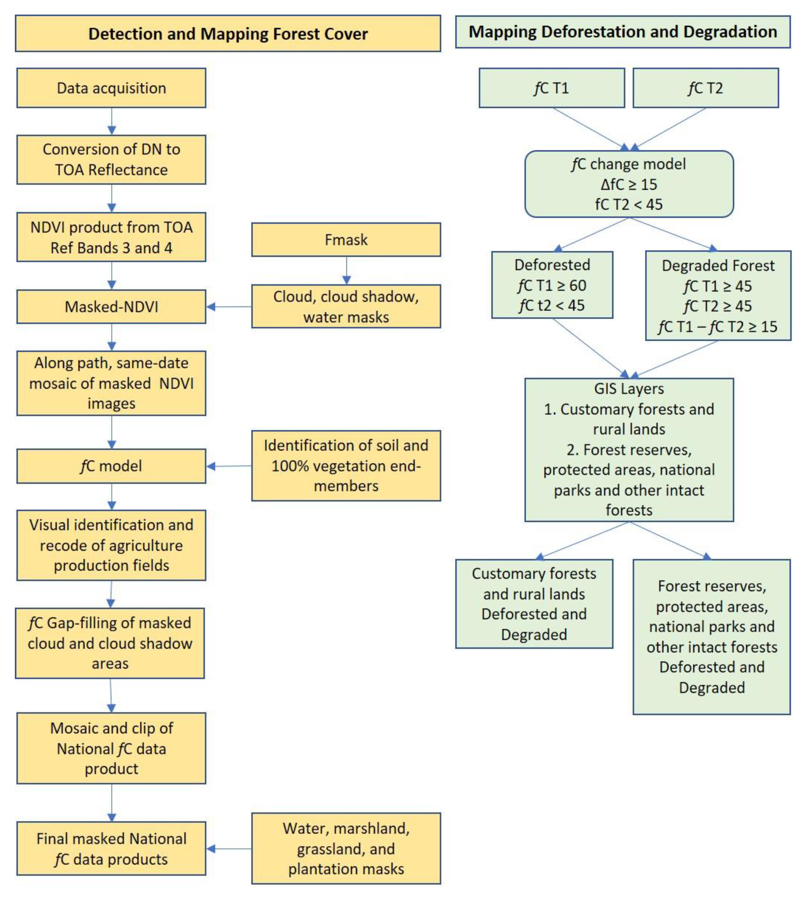
2.3. Data Processing

The fC Tool is a method for using remote sensing data and specific algorithms to produce forest cover maps along continuous fields (Figure A1). Most forest and land cover maps from satellite remote sensing are based on discrete classes of forest or land cover, represented as homogeneous polygons of a single cover type. The continuous fields approach produces land and forest cover maps with robust gradients of cover, more accurately representing natural and anthropogenic variations within cover types. Without a continuous fields approach it is not possible to measure carbon stock degradation or capture natural variations in carbon stocks within forest cover classes. The fC Tool produces forest fractional cover, fC, which is a measure of the fractional cover in forest vegetation, ranging from 0 to 100 percent. It maps variations in these fractional cover values to represent variation in the landscape of forest density, and changes in these fractional cover values to represent various intensities of degradation and deforestation. It is produced from 30 m resolution Landsat data, which are free to the user, to produce a spatial product at a landscape scale relevant to the scale of the disturbance regime in Malawi, and useful for community-based interventions and forest management planning.
We use 30 m Landsat TM, ETM+ and OLI data for three dates, 2000, 2009 and 2015, to detect and map changes in Miombo woodlands in Malawi. The analysis derives vegetation continuous field fractional cover (fC) data products for the whole of Malawi and computes pixel-level changes through a spatially explicit rule model (Figure A1). The fC products are used to map deforestation and forest degradation inside national forest reserves and also in customary land outside of the forest reserves.
The acquisition of Landsat data was based on the following criteria: (1) WRS2 path row images for complete coverage, wall to wall, of Malawi, (2) three years of analysis, 2000, 2009 and 2015 plus or minus two years from the target year, with a preference for along path, same date imagery, (3) seasonal phenology in the early dry season prior to leaf senescence with reduced agricultural field productivity (months of April–June), and (4) minimal cloud cover. For path row images where clouds were present, we acquired multiple images to be used for gap-filling. Fifty-eight (58) images covering 11 WRS2 path/row combinations at three dates were used to provide complete cloud-free coverage of the country (Table 1). All data were level 1G or 1T and acquired through the United States Geologic Service’s Eros Data Center.
The data analysis workflow included seven processing steps: Level 1 digital number (DN) data were converted to top of atmosphere reflectance (TOA) values using [52]. TOA reflectance NIR and Red bands were used to produce an NDVI (Normalized Difference Vegetation Index) product. We created a vegetation continuous-field, fractional cover (fC) product from the NDVI data using a two endmember, linear un-mixing algorithm following [35,37]. We identified cloud and cloud shadow pixels in each path/row scene using the Fmask software [53,54] and then masked these “contaminated” pixels from each path/row image. The national fC product was then developed by gap-filling, mosaicking path/row images, and clipping the mosaicked data to the Malawi border for each target year. This product was then adjusted by masking pixels of no-data, wetland, marsh, grasslands, plantations and water bodies. A two-date fC change detection analysis was performed for the periods 2000–2010 and 2010–2015, which produced national ∆fC change intensity. This was performed for woodland forest areas within protected areas, village forest areas (VFAs) and other customary forests, and trees outside of forest (ToF).
We used the constants and radiometric calibration procedure for each sensor (TM, ETM+ and OLI) provided in [52]. This pre-requisite step of radiometric characterization and calibration is known to produce higher quality “down-stream” products, by reducing errors in observed Earth surface changes from sensor artifacts when using long-term series of remote sensing data for scientific information [55]. The computation for the spectral radiance at the sensor’s aperture uses scene specific metadata that accompanies each set of spectral bands when data are acquired from the USGS EROS Data Center. These constants are also noted in a series of tables in [52]. The conversion of at-sensor spectral radiance to exo-atmospheric TOA reflectance reduces the scene-to-scene variability. Conversion to TOA reflectance uses scene specific data related to the date of acquisition and position relative to the sun’s position at the time of acquisition. The conversion from level 1, digital numbers (DNs) data to at-sensor spectral radiance and then to TOA reflectance is performed for each spectral band for each acquired image.
Normalized Difference Vegetation Index data products are created using the NIR and Red TOA reflectance bands [56]. The NDVI product is a measure of vegetation across the landscape with values between −1 and 1. NDVI pixel values closer to one contain vegetation with high photosynthetic capacity. The equation for NDVI is (NIR − Red)/(NIR + RED).
The detection of pixels “contaminated” by cloud and cloud shadow is accomplished with the “Function of mask” or Fmask series of algorithms first developed by [53] and later improved by [54]. Fmask runs as a DOS prompt executable and processes data through a series of algorithms that identify Landsat pixels as clear-sky, cloud, cloud shadow, water and ice. Missing pixels from the cloud removal are gap-filled with clear sky pixels from other, overlapping data to create a near complete cloud-free landscape for all of Malawi. Recoding was performed for specific agricultural areas in Malawi where irrigated lands included growing crops at the date of acquisition. Pixels in these areas that showed a high fC value were recoded to a value of 0 but included in the deforestation analysis if they were forest at a previous date. A wetland mask was also used to exclude marsh vegetation mapped as high fC. Several data sets were used to mask non-forest areas: these include an internally consistent water mask used across all three dates, grassland, marsh/wetland, and tree plantations.

2.4. Deforestation and Forest Degradation Models

Vegetation continuous field fractional cover (fC) data products are generated from the NDVI data using a two end-member, linear un-mixing algorithm (Figure 2 and Figure 3 and Figure A1). The algorithm uses two end-members representing pure soil (VIsoil) and 100% closed canopy vegetation (VIforest) [35,36,37]. The end-members are selected using an AOI tool through expert knowledge visual analysis for each Landsat NDVI image or along-path mosaic paired with a histogram stretched RGB three-band false-color composite image. Several AOI samples are selected for each end-member throughout an image. The minimum, maximum, mean, and standard deviation are computed from the AOI end-member samples. Along path (same date) and individual scene fC products are created using the minimum, maximum and average end-member values and each are evaluated for path-to-path and gap-filling consistency prior to selection for mosaicking and gap-filling. The fC data are produced as thematic integers and scaled 0 to 100. The fC algorithm is specified as follows: (NDVI − VIsoil)/(VIforest − VIsoil). Figure 2 and Figure 3 present an example of the fC product. The final version of the along-path and individual Landsat fC products are then mosaicked and clipped to the national boundary of Malawi.
Each year-date is referred to as an observation year (OY). Change detection between three OY data layers of national fC is used to measure and map deforestation and forest degradation. Each OY fC data layer and change-intensity ∆fC products are created using separate models for deforestation and forest degradation specified as fC(OYt+1 − OYt). The deforestation and forest degradation models identify pixels that meet pre-defined threshold and criteria in terms of fC values when comparing one date to a second date. These are spatially explicit models written in ERDAS Imagine modeling language. Two input data sets fCt and fCt+1 are compared. The quantitative subtraction of two values produces a continuous field of ∆fC which is the change intensity value (Figure 2).
An initial evaluation of the value of ∆fC is made to test for a minimum magnitude of change, which accommodates for normal variation in fC values unrelated to disturbance (e.g., phenology). All pixels with ∆fC > 15 are considered change cases. Deforested pixels are those where fCt > 45 and fCt+1 < 45. Forest degradation occurs when the pixel value of fCt > 45 and in the fCt+1 > 45. Because of the continuous fields characteristic of the fC change detection, we can map the magnitude of change, ∆fC, which we refer to as change intensity. This change intensity mapping is demonstrated in Figure 2B and can be used to measure and map the intensity of forest degradation.

2.5. Delineation of Tree Cover and Forest Base Layer

The analysis uses a base layer of forest cover with which we quantify and map deforestation and forest degradation from the fC product and the change detection products. We define forest extent as all pixels with an fC value greater than or equal to 45. In addition, forests as defined in this analysis include mapped areas larger than 0.1 ha, with a height more than 5 m, which is essentially the Malawi national definition. The types included are Miombo woodlands and other woody systems with canopy cover equal to or greater than 10%. Included are forest reserves, other protected areas such as game parks and national parks, village forest areas, community woodlots, other tree covers in agricultural areas, and clusters of trees outside of forests in customary lands. Our base data layer was measured to have 4.27 × 10⁶ ha of forest. This represents ~45% of the national land area. The value we use includes customary forest, sparce tree covers and closed canopy forests, and thus is larger than some other reported areas. Figure 2 shows a detail section around the Liwonde Forest Reserve and shows how our multi-date change-detection based on ∆fC produces a gradient of change intensities. A national map of forest and tree cover using the fC method is shown in Figure 3 for 2009 and 2015.

3. Results

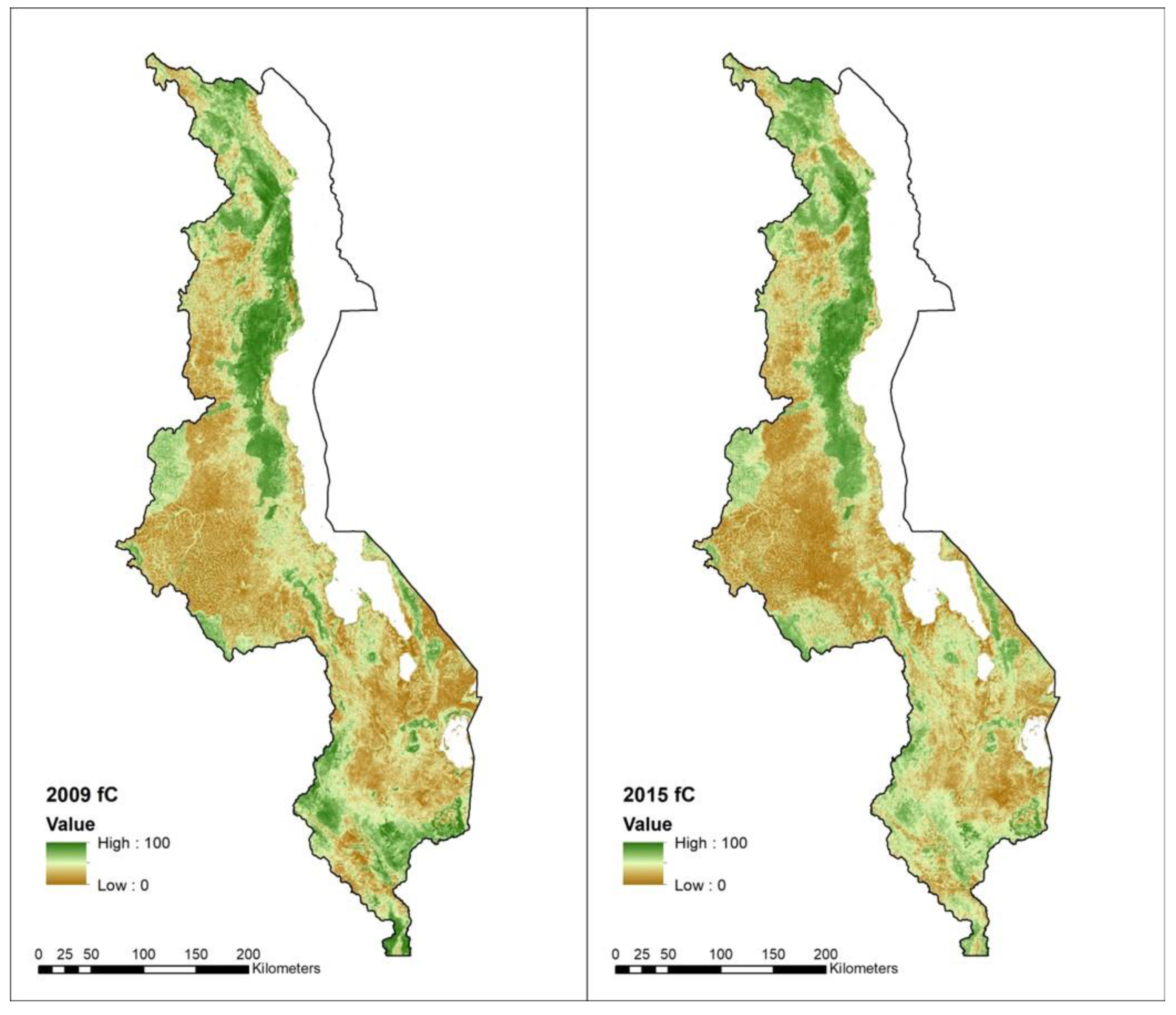
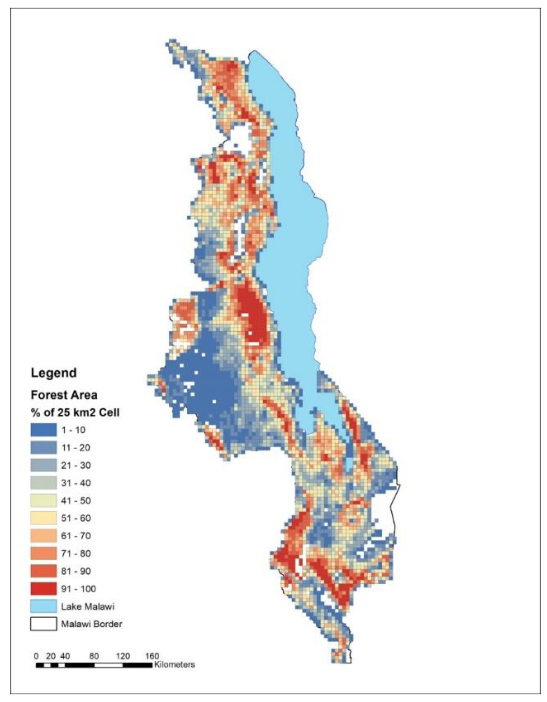
3.1. National Forest Area

Our analysis mapped and quantified the total forested area in forest reserves, other protected forests, customary lands, village forest areas, community woodlots, large agroforestry, and other clusters of trees outside of forest dense enough to qualify as forest by our definition based on minimum fC value (cf. 45). The total area in 2000 was estimated to be 4.27 × 10⁶ ha (Figure 3, Table 2), which includes 2.56 × 10⁶ ha of forests in reserves and protected areas, and 1.70 × 10⁶ ha of customary tree systems, woodlots and village forest areas in customary or rural land. This map was used as a baseline and was reprocessed in 2009 and 2015 to detect areas of deforestation and forest degradation based on the change in forest fractional cover (∆fC).
The forest area definition we use includes small patches of forest greater than 0.1 ha (one pixel) with a density based on fC values great than 45. The Malawi national definition of forest in the reporting of Reference Emission Levels (RELs) to the United Nations Framework Convention on Climate Change uses a patch size of 0.5 hectares. When all patches less than 0.5 ha are eliminated from our dataset, we do not see a significant change in the total forest area nor its distribution. Using a minimum mapping unit (MMU) of 0.5 ha, the total forest area is 4.17 × 10⁶ ha, 98% of our baseline forest area. Table 2 shows the total baseline forest area using different definitions of the minimum area specification. There is only a 4% difference between our MMU and the largest MMU we tested.

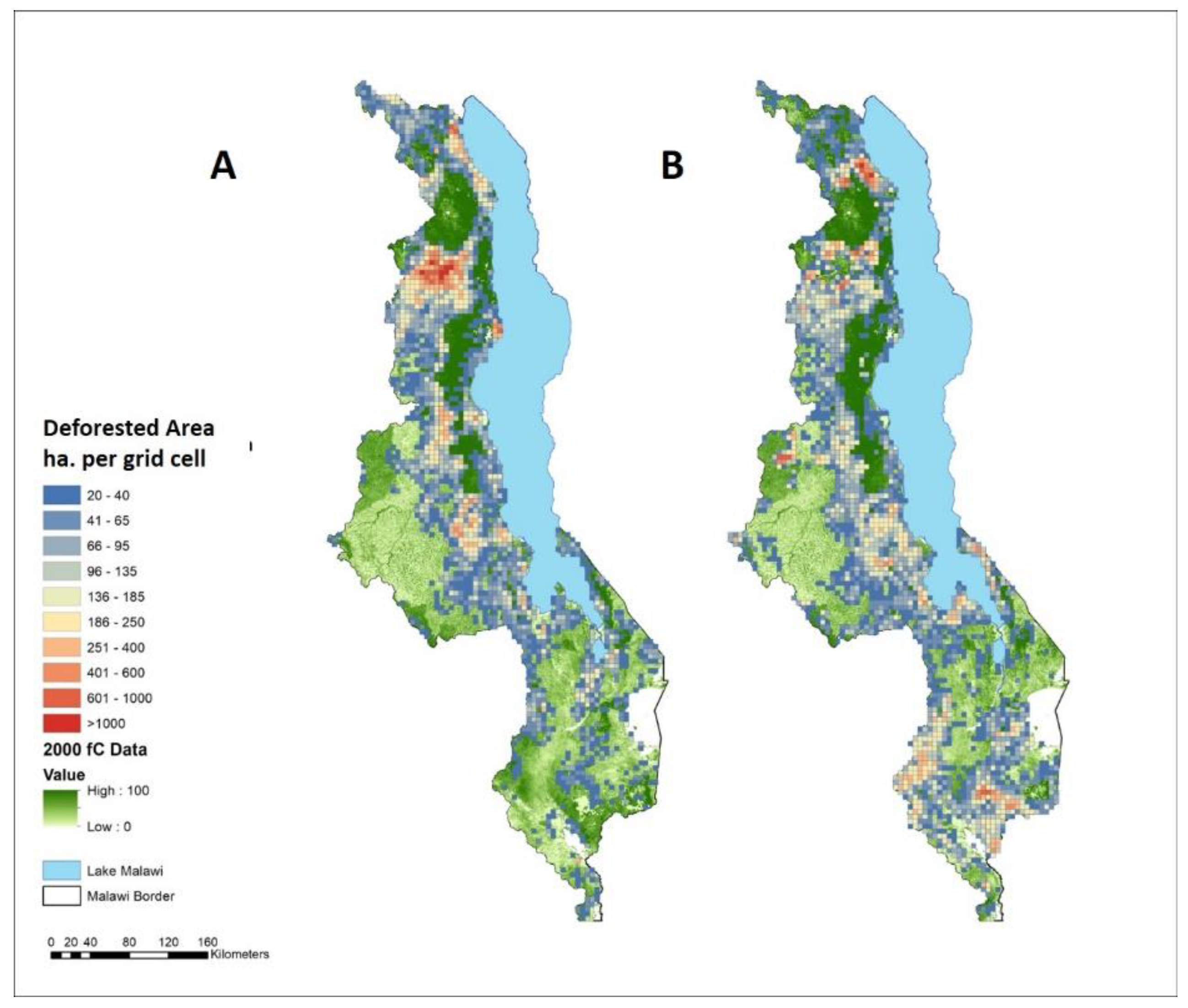
3.2. Deforested Areas and Annual Rates

From 2000 to 2009, the total area deforested, which is the complete conversion of forest to another land cover, was 201,688 ha (Table 3). The average annual rate of deforestation was 22,410 ha yr−1. The area deforested between 2009 and 2015 was slightly higher at 233,624 ha. This is an annual average rate of deforestation of 38,937 ha yr−1. The annual rate of deforestation increased markedly during the study period, with the rate increasing by 74% for 2009–2015 over 2000–2009, although we do not have interannual data to evaluate if there were any years that deviated from average rates. Through the study period the total area deforested was 435,312 ha, or 17% of forest area.
Table 3 also shows estimates for deforestation areas and rates in protected areas and other gazetted forests under government management compared to deforestation in customary and other rural land. These results are very interesting in that they portray a marked shift in the location of deforestation over the 15 year period. From 2000 to 2009, 80% of all deforestation occurred in customary woodlots, tree complexes, and forests (162.0 × 10³ ha) compared to 20% (39.7 × 10³ ha) in forest reserves and protected areas. By 2009–2015 only 42% of deforestation occurred in customary landscapes (97.6 × 10³ ha), while fraction of deforestation occurring in forest reserves and protected areas rose to 58% (136.0 × 10³ ha). These results demonstrate the importance of separately mapping forest reserves and rural customary land because the drivers and dynamics are different and change differently over time. Moreover, considerable tree cover loss occurs outside of government-managed areas and contribute to Malawi’s greenhouse gas emissions.

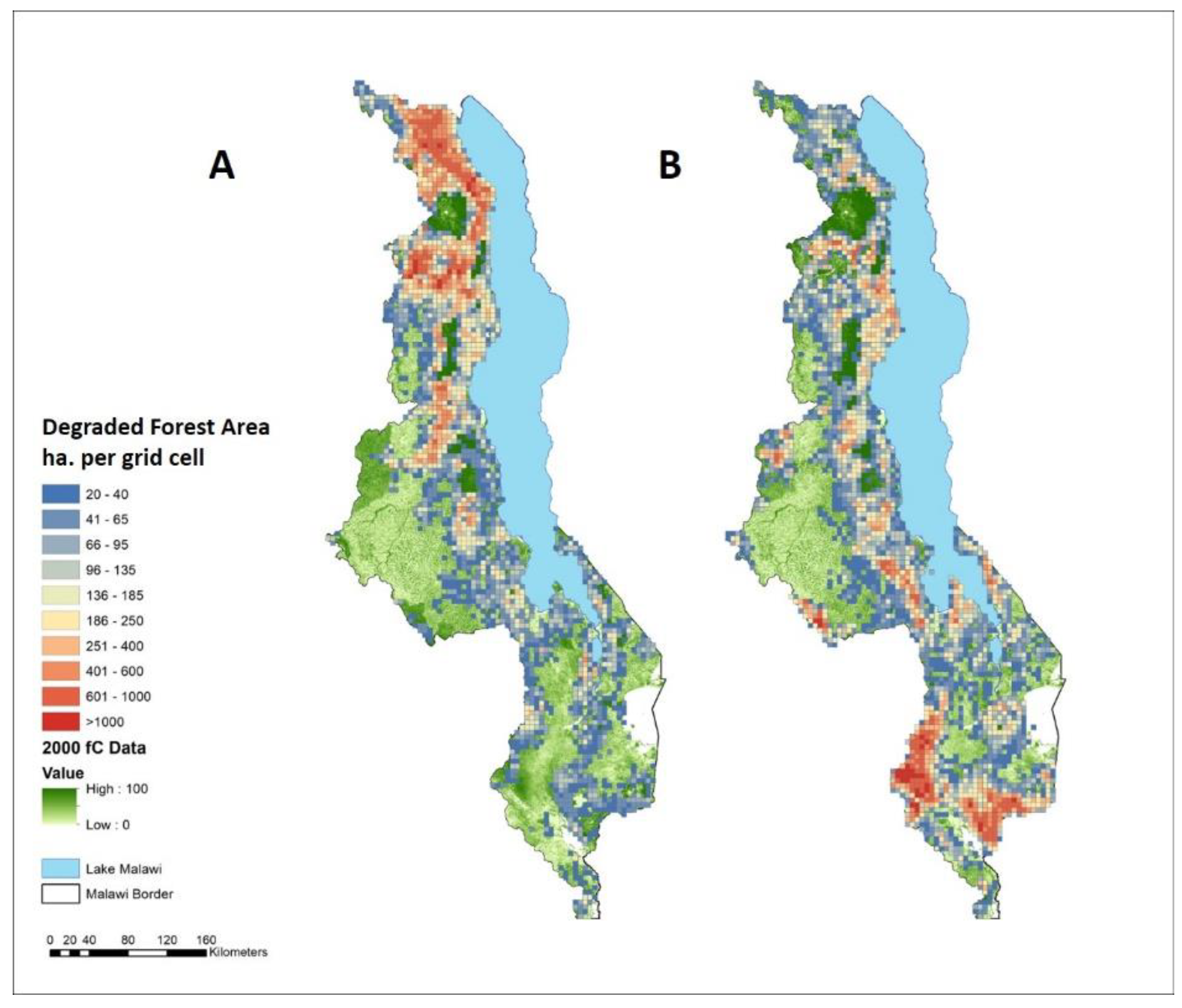
3.3. Forest Degradation Areas and Annual Rates

The total area of forest degradation from 2000 to 2009 was 386,648 ha, and from 2009 to 2015 was 431,266 ha (Table 3). On an average annual basis we estimated forest degradation rates for the period, 2000–2009, to be 42,961 ha yr−1 and from 2009 to 2015 to be 71,878 ha yr−1. Unlike deforestation, forest degradation has always been highest in forest reserves and other government managed areas: 64% of all degradation detected in the period 2000–2009 was in government managed areas, increasing to 72% in 2009–2015. Forest degradation exceeds deforestation throughout the time series, and by a significant amount in some locations when examined as a map. In the period 2000–2009, forest degradation was 92% higher than deforestation, and 2009–2015 forest degradation was 85% higher. It is notable that in the period 2000–2009, forest degradation rates were 6-fold higher than deforestation in forest reserves, declining considerably to 2-fold during the period 2009–2015. Generally, in customary and other rural landscapes deforested area and degraded areas and rates were quantitatively approximately equal, but in the early period deforestation areas and rates slightly exceed forest degradation areas and rates. Thus, currently forest degradation is the dominant form of anthropogenic forest cover disturbance.
The combined disturbance from deforestation and forest degradation from 2000 to 2009 was 588,336 ha, and from 2009 to 2015 was 664,890 ha an increase of 13%. Total forest disturbance for the entire period was 1,253,226 ha.

3.4. Analysis by District

When deforestation and forest degradation rates are examined by district, we see a general shift in the location of these disturbances from the northern districts to the southern districts (Table 4). For both deforestation and forest degradation, the districts in the north generally declined during the second period, while districts in the south generally increased. For the most part, all districts had higher degradation rates than deforestation rates. These regional characteristics reflect some significant hot spots at the district level. In the north Mzimba District had the highest levels of disturbance, with the highest deforestation levels in the country. In the south the districts of Mangochi, Thyolo and Chikwawa were important hot spots, with the latter presenting the highest forest degradation levels in the country. The districts of Kasungu, Nkhotakota and Salima represented the Central regions hot spots.

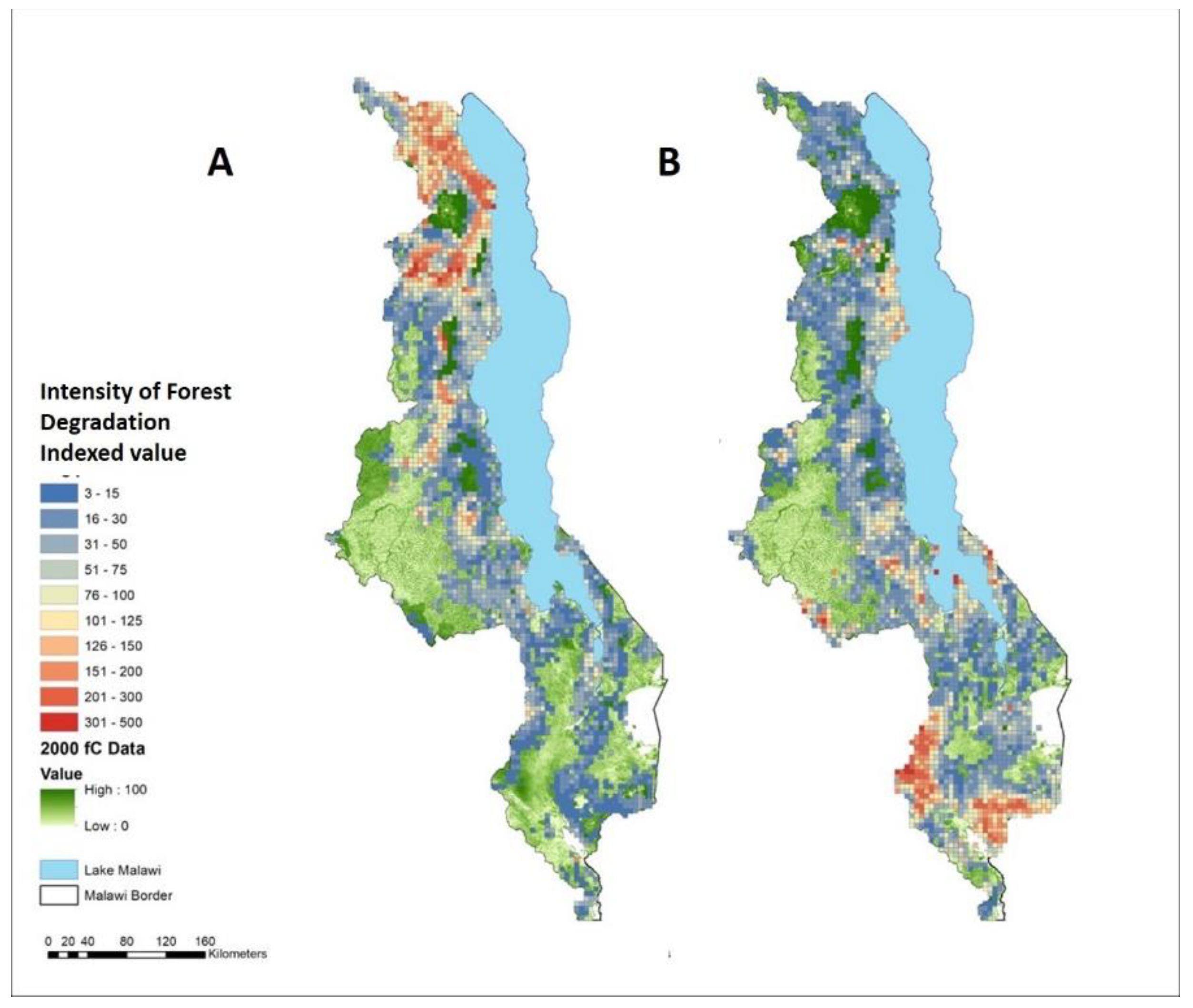
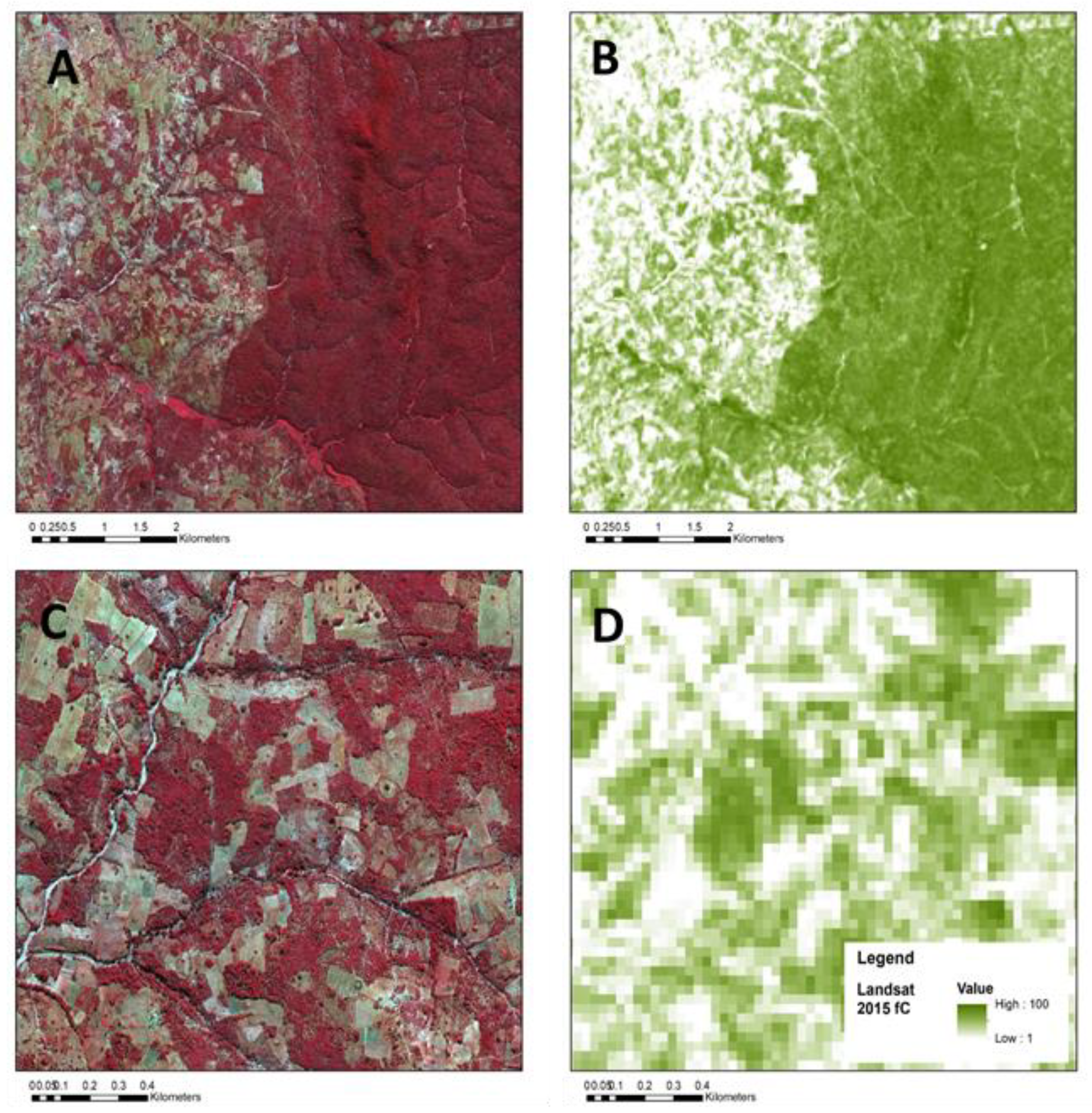
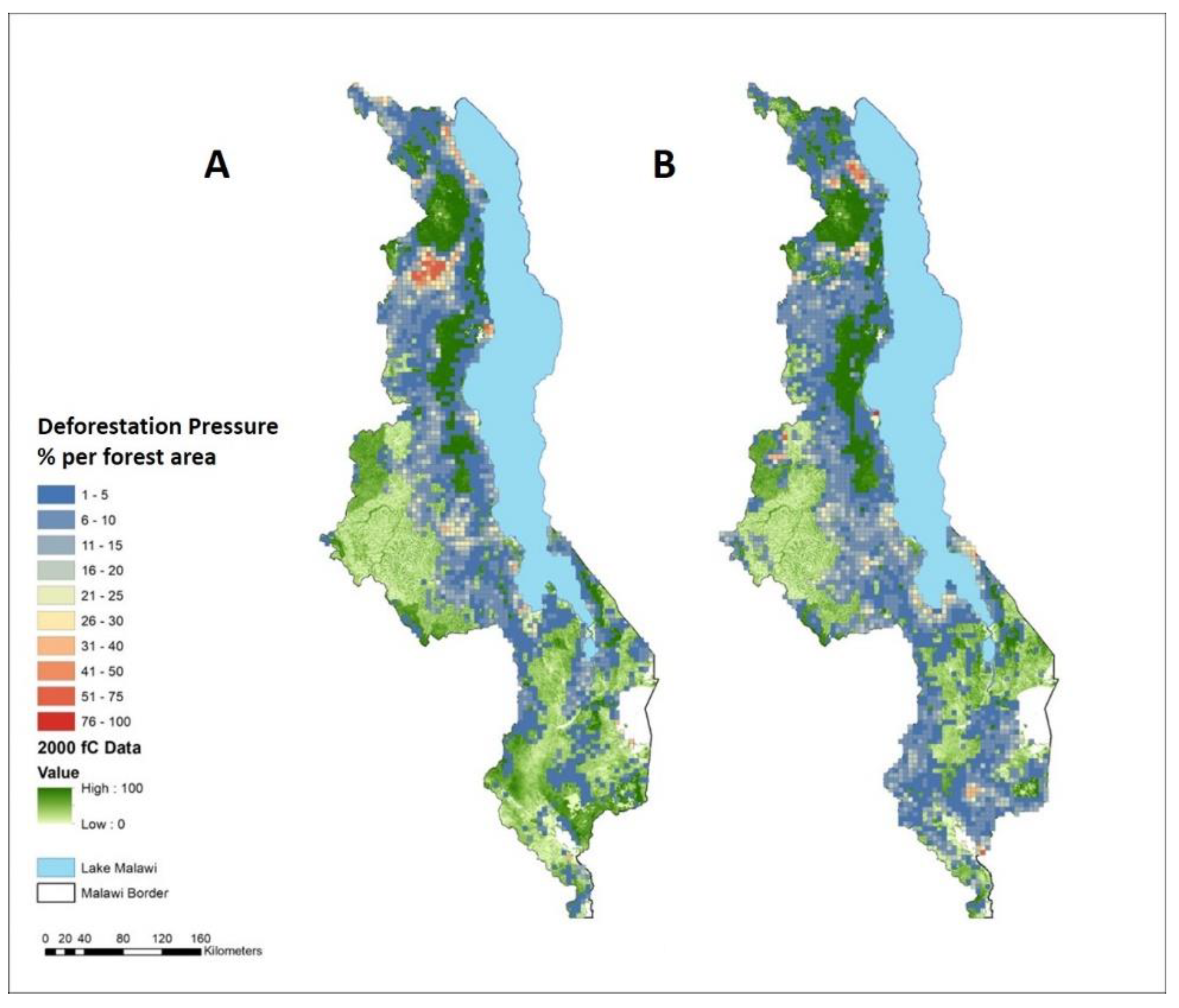
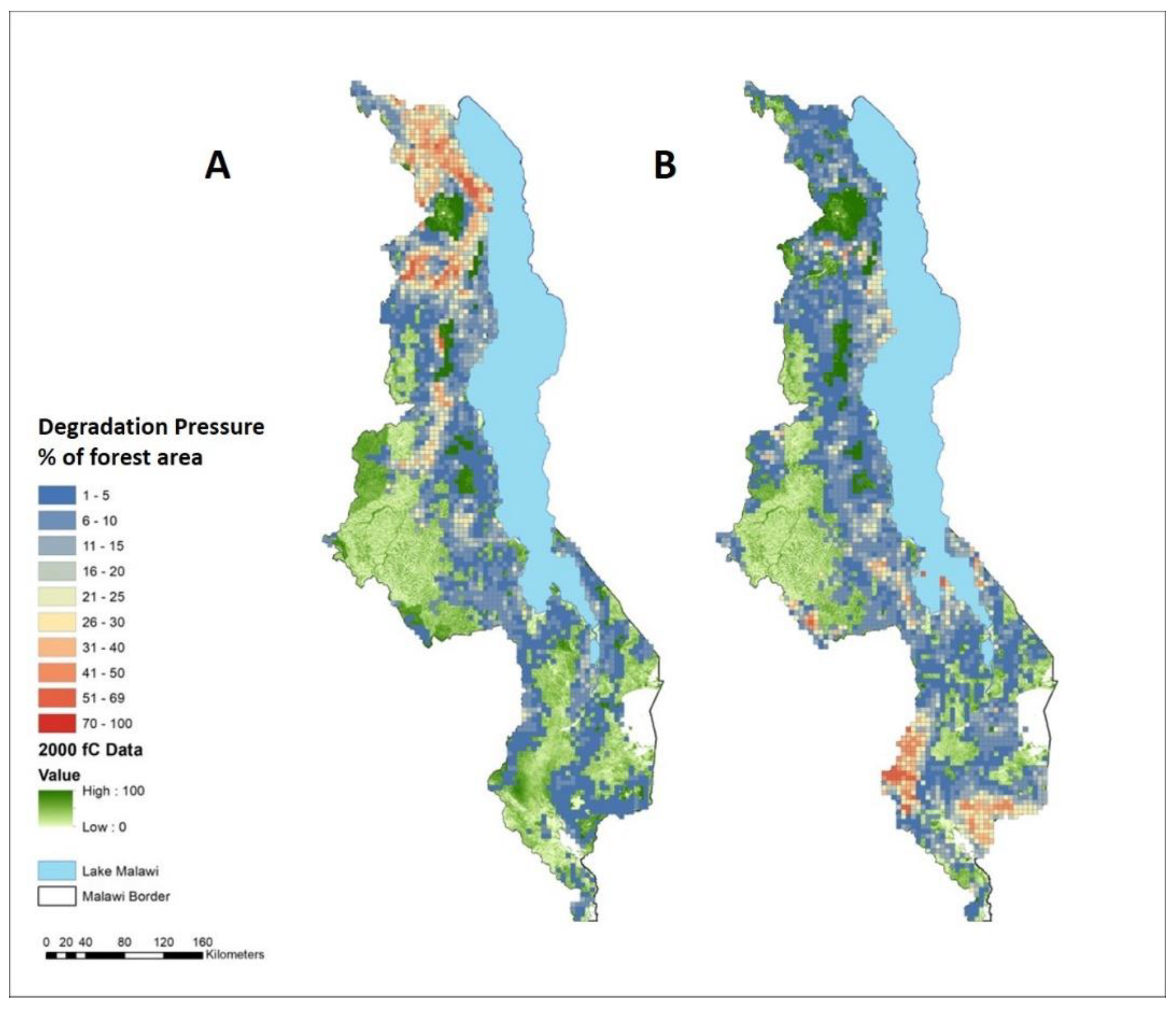
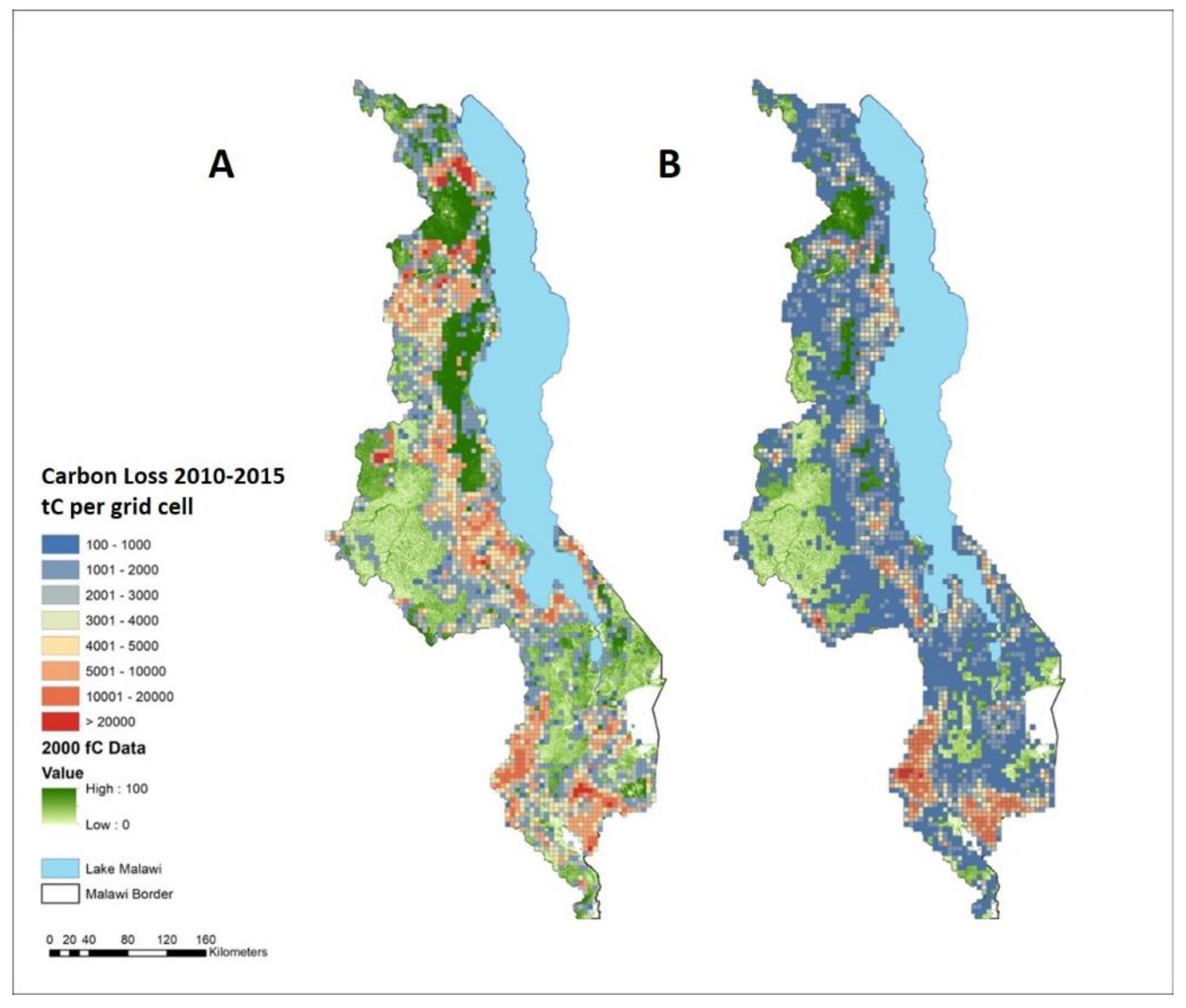
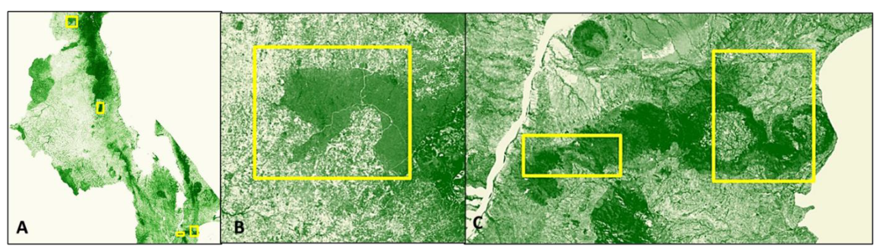
3.5. Mapping and Spatial Analysis

The analysis using remote sensing provides a mechanism to map forest and forest cover change with considerable spatial detail over the entire country. We have two basic formats of our spatial datasets. In the first we present the direct measurement of continuous fields as products from the fC analysis. This spatial dataset can be inspected at the landscape level, at the full 30 m spatial resolution of the fC product (Figure 2 and Figure 3). Disturbance intensity shows the degree of disturbance and is the primary tool for mapping forest degradation. The use of a pixel mixing models allows each pixel’s representation to reflect the sub-pixel fractions of cover. Figure 2A illustrates this point. This is a display of the map derived around the Liwonde Forest Reserve and reveals the continuous fields delineation of forest and woodland density (shades of green). The use of multi-date ∆fC allows for mapping the magnitude, or intensity, of change (color tones, blue/green as low to yellow/red as high). Figure 2B shows this map as a change intensity where the highest intensities represent complete forest conversion (deforestation) while the lower intensities represent forest degradation. The continuous results are split into separate classes for degraded areas and deforested areas. Based on a measure of intensity of change, the spatial dataset can be used to locate specific “hot spots” of deforestation or degradation.
A second mapping product is produced by aggregating 30 m resolution pixels into grid cells of 25 km2 for presenting national coverage in documents. Figure 4 shows the fractional cover map of baseline forest cover for this study. The northern region of Malawi has considerably more forest cover than the other regions of the country, although there are isolated areas with important dense Miombo woodlands throughout the country. Dense forest cover above 75% (fC > 75) of each 25 km2 grid cell exists only in isolated clusters, most of which are forest reserves and other protected areas under government management. To map nationally the magnitude of deforestation, we computed at the pixel level the change in fC (∆fC) between dates, and all pixels that drop fC levels below 45 are considered deforested and aggregated to the 25 km2 grid cell and presented (Figure 5). Not surprising many of the areas of high deforestation are also areas of high forest cover. There are definite hot spots of deforestation in both periods of time, and these have shifted south over the course of the 15 years of analysis. Spatially, deforestation expands considerably into the agricultural landscapes in the second period of analysis, even while the annual rate remains almost constant (Table 3).
The national situation for forest degradation can be examined in a map produced when ∆fC is between 15 and 55 with the final fC value is equal to or exceeds 45 (Figure 6). Forest degradation also expands considerably into agricultural landscapes, while increasing only slightly in magnitude (Table 3). However, it increases more in forest reserves and intact forests, also expanding considerably to the south of the country.
As noted, forest degradation can occur as a gradient of change, within an intensity range. Higher forest degradation has higher impact on carbon stocks. To spatially quantify the impact of forest degradation we used the continuous field and compute an index of degradation intensity for each 25 km2 grid cell, where the reported value is based on the magnitude of the change in fC (∆fC) at each pixel and summed for the cell (Figure 7). The intensity gives us a perspective on how severe the degradation is over time and place. The map shows hot spots of higher-intensity degradation, but generally most of the country has uniform moderate degradation intensities. Over time, there has been a significant shift from north to south in the location of high-intensity degradation.

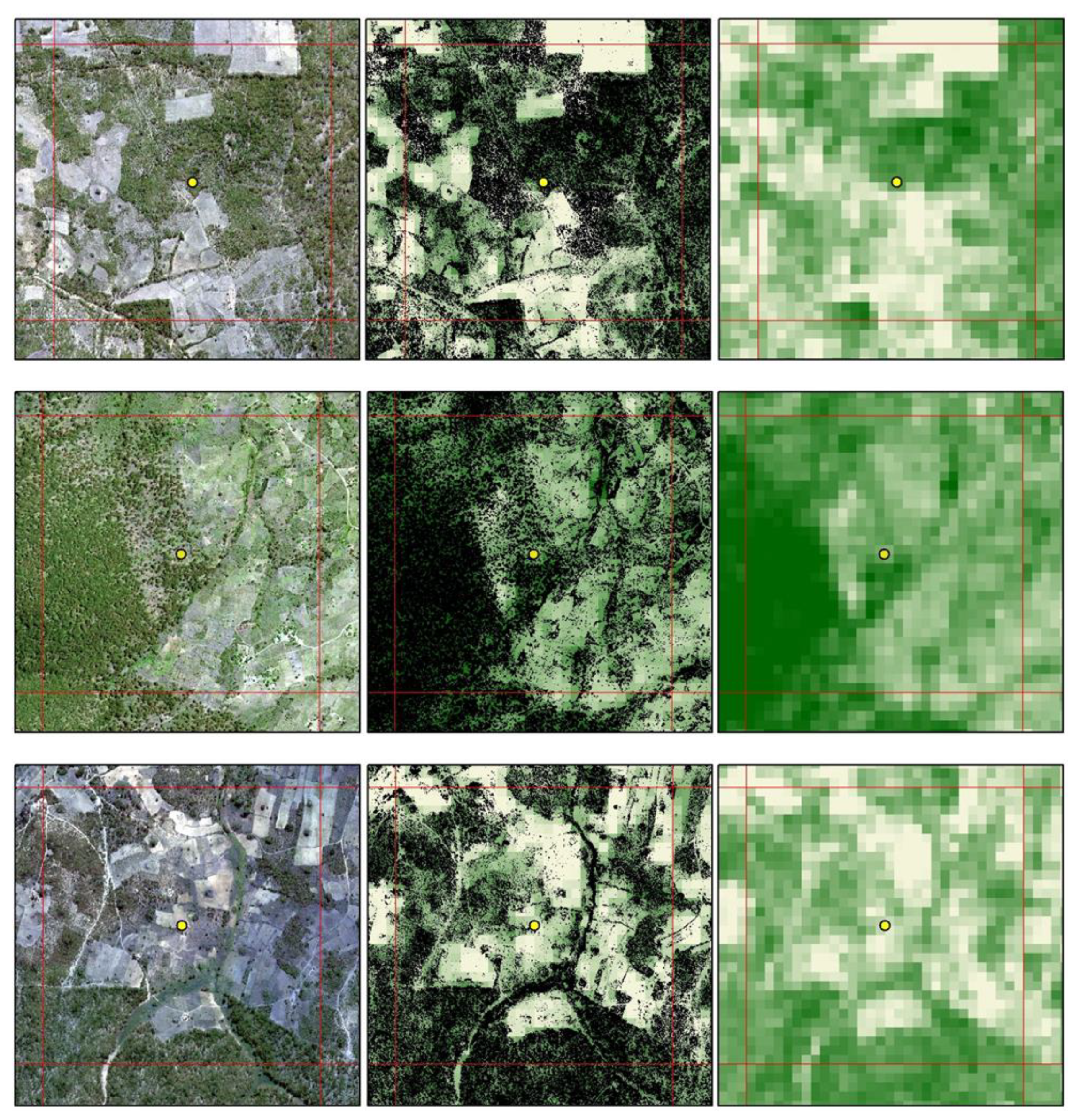
3.6. Accuracy Analysis and Quality Control

A detailed visual inspection of the forest cover product suggests that it well represents features in the landscape when we compare it to hyperspatial resolution imagery, as shown in Figure 8. We made a more quantitative assessment of the accuracy of the fC forest cover product using three analyses described in Appendix A (Figure A2, Figure A3 and Figure A4). In the first analysis we used hyperspatial resolution data to map the forest in the landscape and compare the quantitative estimates of forest cover by the fC product aggregated at the pixel level into a 80 ha grid overlay in three test landscapes in and around the Perekezi and Liwonde forest reserves (Figure A2). There was very good agreement between the independent estimate of forest area from hyperspatial mapping at 0.5 m resolution and the predicted estimate from the Landsat fC product, with linear regression R2 of approximately 0.9 or better (Figure A4).
In the second analysis we overlaid the fC product against a sample of ground validation plots. We deployed 346 30 m fixed radius plots to measure tree cover, tree density, and biomass. A simplified error table was produced for error estimation, suggesting overall accuracy of the fC forest cover product was 93–98% (Table A1).
In a third quantitative analysis, we used hyperspatial satellite data to prepare an fC product in which the fine resolution data (0.5 m) were resampled to the 30 m resolution of our fC product and compared using a standard contingency matrix, as shown in Table A2. Overall accuracy is 84% across all test sites. Producer’s and user’s accuracy were 84% and 94%, respectively, for forest cover mapping. It is important to note that the user’s accuracy, or how often the mapped forest areas are also identified as forests on the ground, is very high (Table A2).

4. Discussion

Most estimates of Malawi’s forest area are reported only for the recorded forest area in government reserves and protected areas, and often include designated forestland that may not contain tree cover at the time of reporting. In spite of recent claims that Malawi has the highest rate of deforestation in Southern Africa [57], we find almost no consistent and comprehensive data on the national deforestation rates and location. There is considerably less information available on forest degradation, which is also common across most of Africa [4,58]. There are important policy requirements for quantitative data on Malawi’s forest status, and growing interest in having improved monitoring capacity to support a range of national policies and measures (PAMs), including implementing Malawi’s new National Forest Policy [59], National Forest Landscape Restoration Strategy [60,61], national initiatives for scaling tree-based systems [23], and National Charcoal Strategy [62]. Accurate spatial data (maps) are particularly critical to support Malawi’s full participation in the United Nations Framework Convention on Climate Change, including its Nationally Determined Contributions [63], National Forest Reference Emission Levels [31], and REDD+ National Forest Monitoring System [47,57,59]. Having capacity for a National Forest Monitoring System is necessary for receiving performance-based payments.
There have been several previous remote sensing mapping exercises that have taken a broad examination of Malawi’s forests but based on a thorough review by [64] these products are highly variable and inconsistent in estimating national forest cover area, which ranges from 18 to 29% of the country area. Forest area in these studies ranged from 2.15–3.49 × 10⁶ ha in 2010. The minimum mapping unit for these analyses is much larger than our study, representing MMUs as large as 25–100 ha. In these reports no attempt was made to explicitly quantify forest cover outside of the recorded forest area (reserves and protected areas) or to include tree clusters, woodlots, agroforestry and village forests on agricultural or customary land. Our analysis reports area estimates that are comparable to these previous estimates for 2010 if we only use the area of forest cover confined to the forest reserves (2.52 × 10⁶ ha for this study), but we have considerably higher estimates overall because we include forests and tree cover on customary and rural land outside of the recorded forest areas (4.27 × 10⁶ ha).
Estimates for the rate of deforestation during the period of our analysis range from ~6 × 10³ ha yr−1 to 30 × 103 ha yr−1 [49,65,66], while our estimate ranges from 22 × 103 ha yr−1 to 39 × 103 ha yr−1. The Global Forest Watch (GFW) estimated total deforested area (i.e., total converted tree cover) between 2001 and 2009 of 51.8 × 10³ ha. Our measurement for the same period was 201.7 × 10³ ha, almost four-fold higher (Table 3). Likewise, the GFW estimates for total deforested area between 2010 and 2015 was 60.7 × 10³ ha compared to our estimate of 233.6 × 10³ ha. These differences are most apparent over the entire period of analysis, 2000–2015 where our measurement of the total area deforested is 435.3 × 10³ ha, which is considerably higher than GFW (Table 3). The most likely explanation for the difference is perhaps the consideration of deforestation in rural and customary land in addition to the contiguous forests of the national reserves and parks, which constitute 60% of our measurement of deforestation. These areas of customary forests, village forests, woodlots and agroforestry are abundant but are widely scattered and do not constitute an extensive and continuous canopy and are thus features that may get removed when processing medium resolution imagery. It has been known that there is substantial tree cover in areas outside of national parks and reserves [66] and informal evidence that tree-based systems are increasing [23,60]. Our measurements suggest that 40% of the national forest cover is on customary or other rural land, which is consistent with [49] who report 42% of forest cover is in trees outside of forests.
The contribution of customary forests is important, but quantitative information has heretofore been hard to find. Some customary forests have been officially designated as Village Forest Areas (VFAs) which are supervised by traditional authorities and managed by Village National Resources Management Committees (VNRMC). The VFAs are important tools for sustainable land management and conservation of public forestlands. However, only a small number of VFA have been registered, and fewer have been surveyed. The exact area and cadastral information do not readily exist [66]. The fC Tool used in this analysis could be deployed to create an inventory and monitoring framework for VFAs, although information concerning species would be difficult. Further investigation of this potential could be productive; supplementing this with very high-resolution (VHR) imagery (Figure A3) might be required.
Our analysis suggests that rates of deforestation are increasing, although the location of the deforestation has notably shifted away from customary forests to public forests (Table 3). There is some indication from informal reports that rates of deforestation during the period prior to 2000 were higher, particularly during the period of one-party government under Hastings Banda. One widely cited assessment [67], which was used in the FAOs Forest Outlook Studies in Africa, reports very high estimates, and that 2.5 × 10⁶ ha of forests were cleared in total, or 125 × 103 ha yr−1, between 1972 and 1992. It is difficult to evaluate these large estimates because no formal study was published, and the methods and definitions are unclear. We know that it was a two-date analysis using Landsat MSS and TM data, so it is quite possible that the results included areas of heavy forest degradation in addition to deforestation. Additionally, possible effects of phenology could have introduced errors because the Landsat collection was not very large, and older coarse resolution MSS data would be difficult to use for this application.
The Malawi State of the Environment and Outlook Report from 2010 [66] reports deforestation rates during the period after the formation of multi-party government. From 1992 to 2010, forest cover change is reported at five-year intervals, with annual deforestation rates at a constant 33 × 103 ha yr−1. Whether rates were exceptionally high in the 1970s and 1980s and declined thereafter, as these reports suggest, is difficult to evaluate. Thus, we have no reliable long term, multi-decadal record of deforestation in Malawi, but it might be possible to reconstruct a reasonable picture, at least to 1986 using Landsat’s historical archive that extends back to 1975. This would be useful for historical, political and economic development studies.
There have been no national-scale direct measurements of forest degradation for Malawi, although it is likely that past deforestation estimates produced without mapping or direct observations also included areas that were heavily degraded rather than completely cleared. Differences between various reports are likely to be related to the degree to which an estimate includes degraded forest in addition to deforestation, or the degree to which the study included disturbances in customary and agricultural landscapes. The results from our study highlight the importance of having a means to make direct measurements of forest degradation, since most of the forest disturbance is associated with forest degradation; degraded forest is almost 2-fold higher than cleared forest. Most of the forest degradation is occurring in public land (Table 3). In the current set of programs and activities under Malawi’s national REDD+ program, forest degradation rates are estimated indirectly from models of fuelwood demand.
This national example for Malawi suggests that new global datasets for forest cover change [41,65] are likely to have limited application to the national REDD+ MRV requirements for Activity Data. The mapping from Global Forest Watch includes almost no forest loss occurrences in rural and customary land outside of the dense Miombo forests of the public forest. Most of the forest loss in GFW is documented in industrial forests in the zone between Mzimba and Mzuzu. At the same time, degradation within forests is not mapped, which from an area perspective is greater than deforestation. An important aim of a National Forest Monitoring System for REDD+ is to identify important locations of both deforestation and forest degradation to proscribe specific controls and interventions, such as forest landscape restoration (FLR). This requires capacity to monitor drivers and post-intervention tree cover outcomes across whole landscapes, especially outside the public forest estate. The dense time series that are provided by these “big data” models may be less necessary than improved specificity of landscape-scale tree cover pattern, distribution and status.
Our spatial analysis suggests that in places where the forest resource base has diminished, deforestation and forest degradation has shifted location in response. This changing geography over time appears to have had three components: (1) an increase in the use of forest reserves, especially due to increased deforestation rates, (2) an expansion of the degradation of forests and tree complexes in customary land across an increasingly wider swath of landscape, and (3) a shift in the location of most deforestation and forest degradation from the northern region of the country to the southern region of the country (Figure 5 and Figure 6). Likewise, the intensity, or severity, of degradation has increased and has shifted from north to south, meaning more forests are being degraded and they are being more severely degraded, especially in the south (Figure 7).
We can examine the pressure on the forest resource base by calculating the ratio of deforestation or degradation per unit of forest, localized within a 25 km2 area (Figure 9 and Figure 10). This can be performed spatially which gives a more accurate representation of resource pressure than using nationally aggregate or average estimates. Some areas stand out because they are experiencing significant pressure on their local forests. In terms of both deforestation and particularly degradation forest pressure has declined in the north while increased in the south over the period of record. Commonly though, local pressure on the forest resource from deforestation, and forest degradation is stabilizing, or declining in some places. However, deforestation and forest degradation rates are indeed increasing because the degradation is expanding spatially over more area.
Regions with the highest rates of disturbance are also, generally, areas of highest amount and density of forest cover. This is particularly true for the northern region of the country, during the first period of analysis and the southern region in the second period of analysis. Thus, while the rates of conversion may be high the pressure on the remaining stock of forest may be lower than other places where there is considerable pressure on low density remaining forest. Typically, conservation priority would be placed on these threatened forests. However, from a carbon context, these areas of high forest cover density where relative pressure is lower may also need mitigation because the emissions may be higher from these forests. The usual management proscriptions to conserve areas of vestige forests may not result in emissions reductions compared to conservation of high cover and high-density forests. Therefor a multi-level approach to management will be required that places conservation strategies on endangered forests and high emissions forests.
The Government of Malawi (GoM) has produced its first national forest reference emissions level report [31], in which they use a sampling approach based on visual interpretation of tree cover using Google Earth for deforestation only, limited to forest reserves. Their estimate of the total area deforested between 2006 and 2016 was 88,474 ha. By comparison, our estimate of deforestation for the period 2009–2015 was 233,624 ha, which is considerably higher. The GoM estimate for the annual rate of 8847 ha yr−1 is low compared to our estimate of 38,937 ha yr−1. When we include forest degradation as well, our annual estimate is 12-fold higher at 110,815 ha yr−1. This is a significant difference and will affect calculations of greenhouse gas emissions considerably. Moreover, the GoM reporting does not measure forest degradation directly, but instead uses a model of fuelwood collection derived from proxy estimators rather that direct measurements. The GoM estimated emission from deforestation to be 1.24 × 10⁶ tCO2e yr−1, and 2.99 × 10⁶ tCO2e yr−1 from forest degradation by fuelwood extraction. By contrast, we measure forest degradation directly and in tandem with deforestation so we can separate the two types of disturbance. We can use our spatial datasets to quantify an approximate emissions level using the same simple method deployed by the GoM, and then present the results for deforestation and forest degradation separately and consistently in map form, as shown in Figure 11. Our estimate for deforestation emissions from 2010 to 2015 is 4.28 × 10⁶ tCO2e yr−1 and forest degradation is 3.49 × 10⁶ tCO2e yr−1. These results suggest that the current GoM estimates are low and misrepresented.
The considerable difference in estimates is due to three factors. First, GoM sample approach is very limited in the sample density, where the complete sample frame covered only 27% of the land areas of Malawi, and 61% of the forest area with a sampling density of only 0.04% within the sample frame. Because the spatial distributions of deforestation and forest degradation are not uniform, low sample densities can produce errors. The GoM report does not report an accuracy assessment for the estimated deforestation rates. Further, the low sample frame for rural and customary land eliminates important emission sources from both forest degradation and deforestation. Second, the GoM report uses a minimum mapping unit of 0.5 ha, while we use 0.1 ha. Although the difference between 0.5 and 0.1 MMU does not affect the total forest area estimates, it does have an effect on estimates of change in forest area, i.e., deforestation or forest degradation, underestimating by as much as 40% due to the omission of large number of small disturbances. Third, the use of models based on proxy variables rather than direct measurements may underestimate forest degradation because it does not capture all forms of forest degradation, is limited in geographic scope, and is based on only the wood removals rather than stand disturbance.

5. Conclusions

5.1. New Robust High-Resolution Time-Series Maps of Forest, Deforestation and Forest Degradation Have Been Produced

This study was based on complete national coverage at high spatial resolution (0.1 ha MMU), which provided direct measurements of deforestation and forest degradation, thus avoiding past confusion over rates when forest degradation is omitted or both types of disturbances are co-mingled. A mapping approach may appear to be difficult to implement in many African countries, particularly for forest degradation measurements, so many countries opt-out of including forest degradation in their national REDD+ scope. However, this study demonstrates a practical and accurate modality for implementing direct measurements of forest degradation. The mapping also enhances the utility of the results to proscribe specific local interventions under national polies and measures (PAMs) and for identifying locations and opportunities for forest landscape restoration.
Previous mapping work has been performed in Malawi by various partner organizations. However, these datasets and the technical methods have been limited in meeting the requirements and national needs for REDD+ measurement and monitoring. For example, most of previous products and approaches do not provide measures of forest degradation, which is a critical characteristic of forest cover change in Malawi, where charcoal and fuelwood removals are important drivers of forest degradation. Moreover, most mitigation interventions will be implemented through local-scale changes in forest management, and thus coarse-scale land cover classification maps that do not provide fine scale local information for forest management and planning are inadequate. Detailed, fine-scale maps of forest cover over large areas are needed to identify hot spots of forest degradation where interventions would be most cost-effective. Such detailed maps are also needed to identify hot spots for deploying detailed ground surveys to understand drivers of deforestation and forest degradation. Fine-scale mapping of forest cover change is needed to align with the spatial variation in carbon stocks from ground measurements for accurate GHG emissions and removals estimation.
This study produces new estimates and maps at high spatial resolution of forests in Malawi, which includes public land in reserves and parks as well as customary forests in agricultural area. The forest map adheres closely to the schema developed by the Malawi government but uses a much higher minimum mapping unit that captures considerable amount of important customary forests. The total estimated area of all forests for 2015 is 3.83 × 10⁶ ha, of which 21% is degraded forests.
This study also produces new estimates for the total area deforested between 2000–2009 (201,688) and 2009–2015 (233,624 ha), and new estimates of the rate of deforestation between 2000–2009 (22,410 ha yr−1) and 2009–2015 (38,937 ha yr−1). We further produce new and separate estimates of the total forest degradation between 2000–2009 (386,648 ha) and 2009–2015 (431,266 ha), and new estimates of the rate of forest degradation between 2000–2009 (42,961 ha yr−1) and 2009–2015 (71,878 ha yr−1). The implications of these new estimates for calculating carbon emissions are important. They are approximately 3-fold higher than reported by the GoM, with forest degradation accounting for a large fraction. These new estimates and the associated maps should be of interest to the national REDD community in Malawi and others for both science and policy use.
The current reporting from the GoM of carbon emissions for its national forest reference emission level (FREL) estimation is likely to be insufficient for use in the National REDD program. The current national estimates have been produced without published accuracy assessment. Based on our study, their quantitative results are likely to be low, perhaps by as much as an order of magnitude, due to methodological issues and use of proxy estimators rather than direct measurements. The choice of a MMU will have an important impact on measurement, resulting in underestimates due to the high level of small clearings and disturbances. Although we show that the choice of MMU only slightly affects the total area estimate of forest nationally, computations of change, i.e., deforestation and forest degradation areas and rates, can be very different, as appears to be the case here.

5.2. New Tools to Support a REDD+ National Forest Monitoring System Have Been Demonstrated

These results have implications for National REDD Programs in Malawi. The UNFCCC advises countries that are Parties to the Convention (COP) and are aiming to undertake REDD+ activities to follow specific methodologies for estimating greenhouse gas (GHG) emissions and removals developed by the International Panel on Climate Change (IPCC). These methodologies require a system for estimating forest stocks and fluxes using a national forest monitoring and measurement system (NFMS). Further, the UNFCCC recommend national programs consider their scope of REDD activities from a list of five elements: (1) reducing emissions from deforestation, (2) reducing emissions from forest degradation, (3) conservation of forest carbon, (4) enhancements of forest carbon, and (5) sustainable forest carbon. Determination of the national scope is important because it sets the agenda for national policies and measures (PAMs). All countries participating in REDD+ actions and programs need to have a basic level of “readiness” for implementing a NFMS to produce the data needed for REDD+ measurement, reporting, and verification (MRV). In this study we demonstrate potential for implementing in Malawi four of these scope elements and provide a model for operational components of Malawi’s NFMS.
As with many countries in Africa the establishment of a National Forest Monitoring System (NFMS) is a key challenge in developing its reporting stream under REDD+ and its NDC efforts. Following COP decisions and guidance a NFMS includes three parts, or pillars as sometimes called: (1) a satellite land change monitoring system (SLMS), which includes a national land classification schema and mapping of changes in forest cover due to deforestation and forest degradation, (2) a national forest inventory (NFI) that focuses on carbon stocks from a system of field plots, using standardized methods and field measurement protocols, and (3) routine quantitative estimation of GHG emissions and removals from plot data and forest cover monitoring data over time, benchmarked to reference emission levels (RELs). This study provides a demonstration of how Malawi can bring its NFMS efforts to an operational readiness level with respect to the SLMS and its ability to produce detailed, spatially explicit Activity Data.

5.3. The Way Forward and Next Steps

As Malawi expands its response to climate change through forest management, it will increase its deployment of the National Forest Landscape Restoration programs. Low carbon forest management is an essential component of low emissions development strategies aimed at enhancing livelihoods for millions of Malawians, and thus is an essential climate change adaptation measure as well as mitigation strategy. Furthermore, the country’s commitments to mitigation and adaptation through its Nationally Determined Contributions reports include increasing forest cover by 2% which requires a four-fold increase in reforestation efforts and sequestering up to 2.6 × 10⁶ tCO2e. Most of that would come from FLR activities. Although this analysis focused on deforestation and forest degradation, two important Activity Data emission sources, the approach would also apply to monitoring for FLR for tree cover regeneration over time.
This is a priority for a follow-on analysis. The National Opportunity Assessment for FLR produced in 2017 [61], identified candidate sites for interventions, based on a multi-criteria analysis based on an indirect mapping of forest degradation with proxy data inputs, while our analysis could provide an empirical, evidence-based map of actual forest degradation. Moreover, the FLR Opportunity Assessment was limited in its ability to identify intervention opportunities within forests, where previously degraded forest could be restored with overplanting and other practices. An important next step for this analysis must be the task to map regeneration. With that it will be possible to have a complete accounting of GHG emissions and removals and track the progress toward national climate mitigation goals.
As with many developing countries, the Government of Malawi (GoM) recognizes the general importance of expanding its national capacities to measure and manage its forest resources even without the predicate of REDD+. Indeed, national interests are best met by developing MRV capacities that satisfy carbon requirements of REDD+ and also basic national forest management needs, with as much utilization of capacities already in place or existing elsewhere that could be readily transferred. This strategy is often referred to as a “no regrets REDD” strategy. For most countries in Africa, there is a recognized immediate challenge to increase data collection, improve forest monitoring, develop measurement standards and protocols, define appropriate mitigation measures, and expand overall technical means. An optimal approach would be one that uses current capacities or readily available and tested best practices for making measurements compatible with IPCC guidelines and protocols. This study demonstrates that countries such as Malawi do not have to go elsewhere to acquire their measurements but can readily develop and own the necessary national technical capacity to deliver robust MRV functions from a National Forest Monitoring System.

Author Contributions

Conceptualization, D.L.S., J.H.S., C.M., M.C., T.T. and D.N.; methodology, D.L.S., J.H.S., C.M., M.C., D.N. and T.T.; validation, M.C., D.N., T.T., J.K., D.K., A.C. and F.K.; formal analysis, D.L.S., J.H.S., C.M., M.C., D.N., T.T., D.K., J.K., A.C. and F.K.; data curation, J.H.S.; writing—original draft preparation, D.L.S.; writing—review and editing, D.L.S., J.H.S., C.M., M.C., D.N., T.T., D.K., J.K., A.C. and F.K.; visualization, J.H.S.; supervision, D.L.S., C.M., D.K., J.K. and A.C. All authors have read and agreed to the published version of the manuscript.

Funding

This research was funded by National Aeronautics and Space Administration, Land Cover and Land Use Change Program (LCLUC), grant number 80NSSC21K0315 and 80NSSC20K0263d and the APC was funded by NASA grant 80NSSC21K0315 and Michigan State University.

Data Availability Statement

All results from data analysis needed to evaluate this report are available in the main text or in tables and figures. Primary public domain satellite remote sensing data are available from the U.S. Geological Survey Eros Data Center (EDC) in the United States. The remote sensing–derived products, spatial data layer products, validation data, and Excel spreadsheets of spatial analysis are available from the Tropical Rain Forest Information Center, a NASA ESIP Data Center, now maintained by the Global Observatory for Ecosystem Services at Michigan State University (https://goeslab.us/malawidata (accessed on 30 March 2021)), and from the NASA Land Cover and Land Use Change Program data server (https://lcluc.umd.edu/content/metadata (accessed on 30 March 2020)). Also the GOES map server, https://www.arcgis.com/apps/View/index.html?appid=181b9bdc8ae74b7b9402edb589bb6e93 (accessed on 30 March 2020).

Acknowledgments

We wish to acknowledge the Alliance for African Partnership at Michigan State University for support to the research collaboration and one workshop, as well as the Lilongwe University for Agriculture and Natural Resources for in-kind support for workshops. We acknowledge the U.S. Agency for International Development PERFORM project for graduate student support through early fellowships to Malawi in-service professionals in the Department of Forestry. We acknowledge the Department of Forestry, Ministry of Forests and Natural Resources for supporting researcher participation as well as early comments on the work. We acknowledge the Future Africa Institute at the University of Pretoria for administrative and technical support.

Conflicts of Interest

The authors declare no conflict of interest. The funders had no role in the design of the study; in the collection, analyses, or interpretation of data; in the writing of the manuscript, or in the decision to publish the results.

Appendix A

Appendix A.1. Data Processing

There are several steps to producing a final forest fractional cover product map, within two broad components. In the first component, we process data using a spectral mixting analysis (SMA) based on two linear end-members of NDVI according to Matricardi et al. [37]. In the second component, we use change detection to map the change intensity of fractional forest cover. The steps are shown in Figure A1.
Figure A1. Data processing flow for developing the fC product.
Forests 12 00426 g0a1

Appendix A.2. Accuracy Analysis

The To evaluate the accuracy of the forest cover product used in this analysis, we established five test sites in and around four national forest reserves (FR): Perekezi FR, Ntchisi FR, Liwonde FR and the Thuma-Dedza FR. Within these test sites we had access to ground sample plots acquired in 2015 (except Thuma-Dedza which were acquired in 2017) which provided tree and cover inventory data. Within the test areas we established four testing landscapes that included forests in the FRs and in the surrounding customary land, where we acquired very high-resolution (VHR) satellite data imagery to be used for ground truth (Figure A1).
Figure A2. Location of test sites. Yellow boxes outline the coverage with VHR satellite data. (A) Reference map showing four test sites in Malawi. (B) The landscape in and around the Perekezi Forest Reserve, and the bottom inserts is (C) The landscape in and around the Liwonde Forest Reserve, segmented into east and west test sites.
Forests 12 00426 g0a2
Figure A3. Landscape test sites where digital hyperspatial satellite data are used to produce an fC product and compared to the Landsat fC product. Image on the left is the raw hyperspatial data. Middle image is an tree cover product from hyperspatial data. Image on the right is the Landsat fC product.
Forests 12 00426 g0a3
We tested accuracy using three tiers of analysis. In the first test we overlaid our fC Tool forest cover mapping product on VHR multi-spectral satellite data (<0.5 m resolution) from Worldview. The VHR data were classified into a high resolution, very detailed forest cover maps, in which individual trees could be identified along with tree clusters and closed canopy forest (Figure A2). Using the VHR data we could construct a proxy ground thruth dataset in which we could precisely define forest cover based on our definition and criteria. For both the VHR forest cover map and the fC Tool output product we overlaid a grid mesh of 81 ha (810,000 m2) grid cells, representing a sample landscape (Figure A2). Each grid contained 900 fC product pixels and 3.2 × 10⁶ VHR pixels. In each 81 ha grid cell we summed the total forest cover. Although the fC Tool allows for mapping forest fraction cover we only considered total forest cover based on our definition without respect to density. The results of these two analyses were compared and are shown in Figure A3.
Figure A4. Test site regression analysis to compare the reference forest cover from very high-resolution (VHR) data to the output mapping from the fC Tool. Each data point represents the mapped and estimated forest cover in each 81-hectare grid cell covering the landscape sites shown in Figure A1.
Forests 12 00426 g0a4
These regressions test the coherence of the independent dataset from VHR data and the fC derived dataset. The results indicate high values for the coefficient of determination (R2). Lower values appear for the Ntchisi test site, which is likely due to its much higher density of forest cover and occurrence of other forest types than Miombo, including large establishment of evergreen forest. This suggest the spectral mixing model modulates the results when end-members of soil and non-photosynthetic vegetation are not well represented. However, in other areas, there is good agreement between the two datasets.
A second analysis was performed using a collection of field plots. We deployed 346 30 m fixed radius plots to measure tree cover, tree density, and biomass. We established these plots in preparation of the Malawi National Forest Inventory (NFI) demonstration under the national REDD+ program [27]. Field plots include measurements coincident with our period of analysis (2015) in Liwonde, Ntchisi, and Perekesi forest reserves and surrounding areas (N = 250) and two years later (2017) in Thuma-Dedza (N = 96). Accuracy of the fC forest cover product in the former was 98% and in the latter was 93% (Table A1).
In a third analysis we used digital hyperspatial data classified into forest cover. These 0.5 m resolution data were resampled to 30 m and directly compared to the fractional forest product. The forest threshold was set as an fC value of >45. Large test sites (complete forest reserves) were established in four forest reserves and surrounding landscapes: Liwonde, Ntchisi, Thuma-Dedza and Perekesi (Figure A1). Table A2 shows the summary statistics for accuracy of forest cover mapping. As a forest mapping product overall accuracy is 84% across all sites. Producer’s and user’s accuracy was 84% and 94% for forest cover mapping. It is important to note that the user’s accuracy, or how often the mapped forest areas are also identified as forests on the ground, is very high.
Table A1. The Accuracy of forest cover mapping using the fC method compared to field plots in selected forest reserves.
Liwonde, Perekezi, Ntchisi (2015)
Number of Field Plots—All Forest Areas250
Count
fC2015 ≥ 45 (Forest)245
fC2015 < 45 (non Forest)5
Percent Correct98%
Thuma-Dedza (2017)
Number of Field Plots—All Forest Areas96
Count
fC2015 ≥ 45 (Forest)89
fC2015 < 45 (non Forest)7
Percent Correct93%
Table A2. The accuracy assessment matrix comparing mapped forest cover from the fC product and measurements from a product that used hyperspatial imagery to map cover at 0.5 m resolution and aggregated to the 30 m grid spatial resolution. (data are shown as number of pixel samples).
Landsat 2015Hyperspatial 2015
fC < 45fC ≥ 45SumProducers Accuracy
fC < 45 (non forest)8325193810,26381%
fC ≥ 45 (forest)560529,88235,48784%
Sum13,93031,82038,207
Users Accuracy60%94%
n=45,750
Overall Accuracy84%

References

  1. Hosonuma, N.; Herold, M.; De Sy, V.; De Fries, R.S.; Brockhaus, M.; Verchot, L.; Angelsen, A.; Romijn, E. An assessment of deforestation and forest degradation drivers in developing countries. Environ. Res. Lett. 2012, 7, 1–12. [Google Scholar] [CrossRef]
  2. McNicol, I.M.; Ryan, C.M.; Mitchard, E.T.A. Carbon losses from deforestation and widespread degradation offset by extensive growth in African woodlands. Nat. Commun. 2018, 9, 1–11. [Google Scholar] [CrossRef]
  3. Bhattarai, S.; Dons, K.; Pant, B. Assessing spatial patterns of forest degradation in dry Miombo woodland in Southern Tanzania. Cogent Environ. Sci. 2020, 6, 1801218. [Google Scholar] [CrossRef]
  4. Gao, Y.; Skutsch, M.; Paneque-Gálvez, J.; Ghilardi, A. Remote sensing of forest degradation: A review. Environ. Res. Lett. 2020, 15, 103001. [Google Scholar] [CrossRef]
  5. Penman, J.; Gytarsky, M.; Hiraishi, T.; Krug, T.; Kruger, D.; Pipatti, R.; Buendia, L.; Miwa, K.; Ngara, T.; Tanabe, K.; et al. Definitions and Methodological Options to Inventory Emissions from Direct Human-Induced Degradation of Forests and Devegetation of Other Vegetation Types; National Greenhouse Gas Inventories Programme, Intergovernmental Panel on Climate Change (IPCC): Geneva, Switzerland, 2013. [Google Scholar]
  6. Watson, R.; Noble, I.R.; Bolin, B.; Ravindranath, N.H.; Verardo, D.J.; Dokken, D.J. (Eds.) Land Use, Land-Use Change, and Forestry; A Special Report of the IPCC; Cambridge University Press: Cambridge, UK, 2000. [Google Scholar]
  7. Shukla, P.R.; Skea, J.; Calvo Buendia, E.; Masson-Delmotte, V.; Pörtner, H.-O.; Roberts, D.C.; Zhai, P.; Slade, R.; Connors, S.; van Diemen, R.; et al. Climate Change and Land: An IPCC Special Report on Climate Change, Desertification, Land Degradation, Sustainable Land Management, Food Security, and Greenhouse Gas Fluxes in Terrestrial Ecosystems; Intergovernmental Panel on Climate Change (IPCC): Geneva, Switzerland, 2019. [Google Scholar]
  8. Ribeiro, N.S.; Katerere, Y.; Chirwa, P.W.; Grundy, I.M. (Eds.) Miombo Woodlands in a Changing Environment: Securing the Resilience and Sustainability of People and Woodlands; Springer: New York, NY, USA, 2020; p. 269. [Google Scholar] [CrossRef]
  9. Kachamba, D.J.; Eid, T.; Gobakken, T. Above-and Belowground Biomass Models for Trees in the Miombo Woodlands of Malawi. Forests 2016, 7, 38. [Google Scholar] [CrossRef] [Green Version]
  10. Missanjo, E.; Kamanga-Thole, G. Estimation of biomass and carbon stock for Miombo Woodland in Dzalanyama Forest Reserve, Malawi. Res. J. Agric. For. Sci. 2015, 3, 7–12. [Google Scholar]
  11. Chidumayo, E.N.; Gumbo, D.J. The Dry Forests and Woodlands of Africa: Managing for Products and Services; Earthscan: London, UK, 2010. [Google Scholar]
  12. Kuyah, S.; Sileshi, G.W.; Njoloma, J.; Mng’Omba, S.; Neufeldt, H. Estimating aboveground tree biomass in three different miombo woodlands and associated land use systems in Malawi. Biomass Bioenergy 2014, 66, 214–222. [Google Scholar] [CrossRef]
  13. Zulu, L.C. The forbidden fuel: Charcoal, urban woodfuel demand and supply dynamics, community forest management and woodfuel policy in Malawi. Energy Policy 2010, 38, 3717–3730. [Google Scholar] [CrossRef]
  14. Sedano, F.; Silva, J.; Machoco, R.; Meque, C.; Sitoe, A.; Ribeiro, N.; Anderson, K.; Ombe, Z.; Baule, S.; Tucker, C.J. The impact of charcoal production on forest degradation: A case study in Tete, Mozambique. Environ. Res. Lett. 2016, 11, 094020. [Google Scholar] [CrossRef]
  15. Sedano, F.; Lisboa, S.N.; Duncanson, L.; Ribeiro, N.; Sitoe, A.; Sahajpal, R.; Hurtt, G.; Tucker, C.J. Monitoring intra and inter annual dynamics of forest degradation from charcoal production in Southern Africa with Sentinel—2 imagery. Int. J. Appl. Earth Obs. Geoinf. 2020, 92, 102184. [Google Scholar] [CrossRef]
  16. Bone, R.A.; Parks, K.E.; Hudson, M.D.; Tsirinzeni, M.; Willcock, S. Deforestation since independence: A quantitative assessment of four decades of land-cover change in Malawi. South. For. J. For. Sci. 2016, 79, 269–275. [Google Scholar] [CrossRef] [Green Version]
  17. Minde, I.J.; Kowero, G.; Ngugi, D.; Luhanga, J. Agricultural Land Expansion and Deforestation in Malawi. For. Trees Livelihoods 2001, 11, 167–182. [Google Scholar] [CrossRef]
  18. Ngwira, S.; Watanabe, T. An Analysis of the Causes of Deforestation in Malawi: A Case of Mwazisi. Land 2019, 8, 48. [Google Scholar] [CrossRef] [Green Version]
  19. Katumbi, N.; Nyengere, J.; Mkandawire, E. Drivers of deforestation and forest degradation in Dzalanyama forest reserve in Malawi. Int. J. Sci. Res. 2015, 6, 889–893. [Google Scholar]
  20. Mbow, C.; Brandt, M.; Ouedraogo, I.; De Leeuw, J.; Marshall, M. What four decades of earth observation tell us about land degradation in the Sahel? Remote Sens. 2015, 7, 4048–4067. [Google Scholar] [CrossRef] [Green Version]
  21. Gumbo, D.; Clendenning, J.; Martius, C.; Moombe, K.; Grundy, I.; Nasi, R.; Mumba, K.Y.; Ribeiro, N.; Kabwe, G.; Petrokofsky, G. How have carbon stocks in central and southern Africa’s miombo woodlands changed over the last 50 years? A systematic map of the evidence. Environ. Évid. 2018, 7, 16. [Google Scholar] [CrossRef] [Green Version]
  22. Chidumayo, E. Management implications of tree growth patterns in miombo woodlands of Zambia. For. Ecol. Manag. 2019, 436, 105–116. [Google Scholar] [CrossRef]
  23. Kundhlande, G.; Winterbottom, R.; Nyoka, B.I.; Reytar, K.; Ha, K.; Behr, D.C. Taking to Scale Tree-Based Systems that Enhance Food Security, Improve Resilience to Climate Change, and Sequester Carbon in Malawi; World Bank PROFOR: Washington, DC, USA, 2017; p. 56. [Google Scholar]
  24. Zomer, R.J.; Neufeldt, H.; Xu, J.; Ahrends, A.; Bossio, D.; Trabucco, A.; Van Noordwijk, M.; Wang, M. Global Tree Cover and Biomass Carbon on Agricultural Land: The contribution of agroforestry to global and national carbon budgets. Sci. Rep. 2016, 6, 29987. [Google Scholar] [CrossRef]
  25. Brandt, M.; Rasmussen, K.; Hiernaux, P.; Herrmann, S.; Tucker, C.J.; Tong, X.; Tian, F.; Mertz, O.; Kergoat, L.; Mbow, C.; et al. Reduction of tree cover in West African woodlands and promotion in semi-arid farmlands. Nat. Geosci. 2018, 11, 328–333. [Google Scholar] [CrossRef] [PubMed]
  26. Mbow, C.; Toensmeier, E.; Brandt, M.; Skole, D.; Dieng, M.; Garrity, D.; Poulter, B. Agroforestry as a solution for multiple climate change challenges in Africa. In Climate Change and Agriculture; Deryng, D., Ed.; Burleigh Dodds Science Publishing: Cambridge, UK, 2020. [Google Scholar]
  27. Stringer, L.C.; Dougill, A.J.; Mkwambisi, D.D.; Dyer, J.C.; Kalaba, F.K.; Mngoli, M. Challenges and opportunities for carbon management in Malawi and Zambia. Carbon Manag. 2012, 3, 159–173. [Google Scholar] [CrossRef] [Green Version]
  28. Gibbs, H.K.; Brown, S.; Niles, J.O.; Foley, J.A. Monitoring and estimating tropical forest carbon stocks: Making REDD a reality. Environ. Res. Lett. 2007, 2, 045023. [Google Scholar] [CrossRef]
  29. Chiotha, S.; Jamu, D.; Nagoli, J.; Likongwe, P.; Chanyenga, T.F. (Eds.) Socio-Ecological Resilience to Climate Change in a Fragile Ecosystem: The Case of the Lake Chilwa Basin, Malawi; Routledge: London, UK, 2018. [Google Scholar]
  30. Mbow, M.; Skole, D.; Dieng, M.; Justice, C.; Kwesha, D.; Mane, L.; El Gamri, M.; Von Vordzogbe, V.; Virji, H. Challenges and Prospects for REDD+ in Africa: Desk Review of REDD+ Implementation in Africa; GLP Report No. 5. GLP-IPO; GLP International Project Office: Copenhagen, Denmark, 2012. [Google Scholar]
  31. GOM. Malawi REDD+ Program National Forest Reference Level; Government of Malawi: Lilongwe, Malawi, 2019. [Google Scholar]
  32. Grainger, A.; Kim, J. Reducing Global Environmental Uncertainties in Reports of Tropical Forest Carbon Fluxes to REDD+ and the Paris Agreement Global Stocktake. Remote Sens. 2020, 12, 2369. [Google Scholar] [CrossRef]
  33. FAO. Voluntary Guidelines on National Forest Monitoring; Food and Agriculture Organization of the United Nations: Rome, Italy, 2017; 62p. [Google Scholar]
  34. Angelsen, A.; Boucher, D.; Brown, S.; Merckx, V.; Streck, C.; Zarin, D. Guidelines for REDD+ Reference Levels: Principles and Recommendations; Meridian Institute: Washington, DC, USA, 2011; 24p. [Google Scholar]
  35. Matricardi, E.A.; Skole, D.L.; Pedlowski, M.A.; Chomentowski, W.; Fernandes, L.C. Assessment of tropical forest degradation by selective logging and fire using Landsat imagery. Remote Sens. Environ. 2010, 114, 1117–1129. [Google Scholar] [CrossRef]
  36. Matricardi, E.A.; Skole, D.L.; Pedlowski, M.A.; Chomentowski, W. Assessment of forest disturbances by selective logging and forest fires in the Brazilian Amazon using Landsat data. Int. J. Remote Sens. 2012, 34, 1057–1086. [Google Scholar] [CrossRef]
  37. Matricardi, E.A.T.; Skole, D.L.; Costa, O.B.; Pedlowski, M.A.; Samek, J.H.; Miguel, E.P. Long-term forest degradation surpasses deforestation in the Brazilian Amazon. Science 2020, 369, 1378–1382. [Google Scholar] [CrossRef] [PubMed]
  38. Bullock, E.L.; Woodcock, C.E.; Souza, C.; Olofsson, P. Satellite-based estimates reveal widespread forest degradation in the Amazon. Glob. Chang. Biol. 2020, 26, 2956–2969. [Google Scholar] [CrossRef]
  39. Goetz, S.J.; Hansen, M.; Houghton, R.A.; Walker, W.; Laporte, N.; Busch, J. Measurement and monitoring needs, capabilities and potential for addressing reduced emissions from deforestation and forest degradation under REDD+. Environ. Res. Lett. 2015, 10, 123001. [Google Scholar] [CrossRef]
  40. Mayes, M.; Mustard, J.; Melillo, J.; Neill, C.; Nyadzi, G. Going beyond the green: Senesced vegetation material predicts basal area and biomass in remote sensing of tree cover conditions in an African tropical dry forest (miombo woodland) landscape. Environ. Res. Lett. 2017, 12, 085004. [Google Scholar] [CrossRef] [Green Version]
  41. Hansen, M.C.; Potapov, P.V.; Moore, R.; Hancher, M.; Turubanova, S.A.; Tyukavina, A.; Thau, D.; Stehman, S.V.; Goetz, S.J.; Loveland, T.R.; et al. High-resolution global maps of 21st-century forest cover change. Science 2013, 342, 850–853. [Google Scholar] [CrossRef] [Green Version]
  42. Melo, J.B.; Ziv, G.; Baker, T.R.; Carreiras, J.M.B.; Pearson, T.R.H.; Vasconcelos, M.J. Striking divergences in Earth Observation products may limit their use for REDD+. Environ. Res. Lett. 2018, 13, 104020. [Google Scholar] [CrossRef]
  43. Skole, D.L.; Cochrane, M.A. Observations of LCLUCC in regional case studies. In Land Change Science: Observing, Monitoring and Understanding Trajectories of Change on the Earth’s Surface; Kluwer Academic Publishers: Dordrecht, The Netherlands, 2004; p. 461. [Google Scholar]
  44. Petersen, R.; Davis, C.; Herold, M.; De Sy, V. Tropical Forest Monitoring: Exploring the Gaps between What Is Required and What Is Possible for Redd+ and Other Initiatives; Working Paper; World Resources Institute: Washington, DC, USA, 2018; 12p. [Google Scholar]
  45. Seymour, F.; Harris, N.L. Reducing tropical deforestation. Science 2019, 365, 756–757. [Google Scholar] [CrossRef] [Green Version]
  46. Campbell, B. (Ed.) The Miombo in Transition; Center for International Forestry Research: Bogor, Indonesia, 1996. [Google Scholar]
  47. World Bank. Malawi Country Environmental Analysis; World Bank: Washington, DC, USA, 2019; 160p. [Google Scholar]
  48. Coutts, C.; Holmes, T.; Jackson, A. Forestry policy, conservation activities, and ecosystem services in the remote Misuku Hills of Malawi. Forests 2019, 10, 1056. [Google Scholar] [CrossRef] [Green Version]
  49. Mauambeta, D.; Chitedze, D.; Mumba, R. Status of Forests and Tree Management in Malawi; Coordination Union for Rehabilitation of the Environment (CURE): Lilongwe, Malawi, 2010. [Google Scholar]
  50. Kamoto, J.; Clarkson, G.; Dorward, P.; Shepherd, D. Doing more harm than good? Community based natural resource management and the neglect of local institutions in policy development. Land Use Policy 2013, 35, 293–301. [Google Scholar] [CrossRef] [Green Version]
  51. FAO. Atlas of Malawi; Food and Agriculture Organization of the United Nations: Rome, Italy, 2013; p. 139. [Google Scholar]
  52. Chander, G.; Markham, B.L.; Helder, D.L. Summary of current radiometric calibration coefficients for Landsat MSS, TM, ETM+, and EO-1 ALI sensors. Remote Sens. Environ. 2009, 113, 893–903. [Google Scholar] [CrossRef]
  53. Zhu, Z.; Woodcock, C.E. Object-Based Cloud and Cloud Shadow Detection in Landsat Imagery. Remote Sens. Environ. 2012, 118, 83–94. [Google Scholar] [CrossRef]
  54. Zhu, Z.; Wang, S.; Woodcock, C.E. Improvement and expansion of the Fmask algorithm: Cloud, cloud shadow, and snow detection for Landsats 4–7, 8, and Sentinel 2 images. Remote Sens. Environ. 2015, 159, 269–277. [Google Scholar] [CrossRef]
  55. Roy, D.P.; Borak, J.S.; Devadiga, S.; Wolfe, R.E.; Zheng, M.; Descloitres, J. The MODIS Land product quality assessment approach. Remote Sens. Environ. 2002, 83, 62–76. [Google Scholar] [CrossRef]
  56. Rouse, J.W.; Haas, R.H.; Shell, J.A.; Deering, D.W. Monitoring vegetation systems in the Great Plains with ERTS-1. In Proceedings of the Third Earth Resources Technology Satellite Symposium, Washington, DC, USA, 10–14 December 1973; Goddard Space Flight Center: Washington, DC, USA, 1973; pp. 309–317. [Google Scholar]
  57. USAID. Malawi Foreign Assistance Act 118/119 Tropical Forest and Biodiversity Analysis; US Agency for International Development: Washington, DC, USA, 2019.
  58. Pearson, T.R.; Brown, S.; Murray, L.; Sidman, G. Greenhouse gas emissions from tropical forest degradation: An underestimated source. Carbon Balance Manag. 2017, 12, 3. [Google Scholar] [CrossRef] [Green Version]
  59. GOM. National Forest Policy; Government of the Republic of Malawi, Department of Forestry: Lilongwe, Malawi, 2016; p. 60.
  60. GOM. National Forest Landscape Restoration Strategy; Government of the Republic of Malawi, The Ministry of Natural Resources, Energy and Mining: Lilongwe, Malawi, 2017; 44p.
  61. GOM. Forest Landscape Restoration Opportunities Assessment for Malawi; Ministry of Natural Resources, Energy and Mining: Lilongwe, Malawi, 2017; 126p.
  62. GOM. National Charcoal Strategy; Government of the Republic of Malawi, The Ministry of Natural Resources, Energy and Mining: Lilongwe, Malawi, 2017; 44p.
  63. GOM. Malawi Submission of its First Nationally Determined Contribution. 2015. Available online: https://www4.unfccc.int/sites/NDCStaging/Pages/All.aspx (accessed on 4 March 2021).
  64. Haack, B.; Mahabir, R.; Kerkering, J. Remote sensing-derived national land cover land use maps: A comparison for Malawi. Geocarto Int. 2014, 30, 270–292. [Google Scholar] [CrossRef]
  65. Global Forest Watch. Forest Monitoring Designed for Action. Available online: https://www.globalforestwatch.org/ (accessed on 23 February 2021).
  66. GOM. Malawi State of Environment and Outlook Report: Environment for Sustainable Economic Growth; Environmental Affairs Department, Ministry of Natural Resources, Energy, and Environment: Lilongwe, Malawi, 2010; 302p.
  67. Kainja, S. Forest Outlook Studies in Africa–Malawi. 2000. Available online: http://www.fao.org/3/a-ab585e.pdf (accessed on 10 January 2021).
Figure 1. Vegetation of Malawi, showing the distribution of forests. The majority of forest is Miombo woodlands, both open and closed forests. This map was generated by the Food and Agriculture Organization of the United Nations (FAO. 2013. Atlas of Malawi Land Cover and Land Use Change, 1990–2010, Rome. 139 pp.) Codes are URB: Built Up, TP: Tree Plantation, AG: Agriculture, TREO: Tree Cover Open, TREC: Tree Cover Closed, SCO: Shrub Cover, HCO: Herbaceous Cover, BS: Bare Land, and WAT: Water Bodies.
Forests 12 00426 g001
Figure 2. The fC model of forest cover and change measures the intensity of forest disturbance as a continuous field of observations. (A) The fC forest cover product for 2015, where shading of green represents a continuous field of forest cover. (B) Using change detection, ∆fC, is computed from two dates and presented as a continuous gradient of change. If the change is significant it is labeled as deforestation. If the change is within the range of fC values for forest, the intensity of degradation can be estimated and mapped as shown here, where tones of blue and green are low-intensity degradation, and tones of orange and red are high-intensity degradation.
Forests 12 00426 g002
Figure 3. The fractional forest cover product for the years 2009 and 2015. The scale represents a continuous field gradient of values for fC, and subtraction of two dates produces a change product, ∆fC, i.e., 2000–2009, 2010–2015.
Forests 12 00426 g003
Figure 4. Mapping of forest cover density aggregated to 25 km2 grid cells. Forest area is represented as a proportion (%) of each 25 km2 grid cell, from low values in blue to high values in red. The data are produced at 30 m resolution, and a large dataset at that resolution is available for the entire country. Aggregation is used for display at this scale.
Forests 12 00426 g004
Figure 5. Mapped areas of deforestation, 2000 to 2009 (A) and 2010 to 2015 (B), as the area of total new deforested land (ha) created during the period within each 25 km2 grid cell. Cells where deforested area is <20 ha are not shown.
Forests 12 00426 g005
Figure 6. Mapped areas of forest degradation, 2000–2009 (A), 2010–2015 (B), as the area of total new degraded forest (ha) created during each period within each 25 km2 grid cell. Cells where degraded area is <20 ha are not shown.
Forests 12 00426 g006
Figure 7. Mapping of degradation intensity, 2000–2009 (A) and 2010–2015 (B). These maps are used to display where degradadtion is most severe. Thus, two cells could have the same area of forest degradation but containg different intensities of degradation. To compute the intesity we use the following equation: ∑ (100 × ∆fC/55)/Af, where the difference in fC values between dates is divided by the maximum amount of degradation weighted against a proxy for biomass emission factors and summed for all pixels in each 25 km2 grid cell. This value is divided by the area of forest in the grid cell. Much degradation is low intensity, but there are some notable areas of more severe degradadtion. Further, over time there is a north to south shift in the location of highest-intensity degradation.
Forests 12 00426 g007
Figure 8. Examples of the fC product compared with very high-resolution (VHR) satellite data at 0.5 m resolution. (A) VHR, wide area perspective, (B) fC product, wide area perspective, (C) VHR, local area perspective, (D) fC product, local area perspective.
Forests 12 00426 g008
Figure 9. Mapping of the pressure on remaining forest resources from deforestation, 2000–2009 (A), 2010–2015 (B). The total area deforested at each date is expressed as a percent fraction of the forest area in each 25 km2 grid cell.
Forests 12 00426 g009
Figure 10. Mapping of the pressure on remaining forest resources from forest degradation 2000–2009 (A), 2010–2015 (B). The total area degraded at each date is expressed as a percent fraction of the forest area in each 26 km2 grid cell.
Forests 12 00426 g010
Figure 11. An estimate of emissions of carbon (106 g C per grid cell) from deforestation (A) and forest degradation (B), 2010–2015. This estimate uses the same method as found in the Government of Malawi’s report on its National Forest Reference Emission Levels [31]. The method follows IPCC guidance in which Emissions = Activity Data × Emission Factors. The Activity Data are produced by this study, and we used Emission Factors from GOM National Forest Reference Emissions Levels report [31].
Forests 12 00426 g011
Table 1. Listing of all Landsat path/row combinations, acquisition date and scene identifier for imagery used in this analysis.
Path/RowYear 2000Year 2010Year 2015
Scene IDAcq. DateScene IDAcq. DateScene IDAcq. Date
167/70LE71670702002146SGS0026 May 2002LT51670702008155JSA0126 May 2008LC81670702015158LGN00
LC81670702014155LGN00
LC81670702015126LGN00
7 June 2015
4 June 2014
6 May 2015
167/71LE71670712002146SGS0026 May 2002LT51670712009157JSA026 June 2009LC81670712015158LGN00
LC81670712014155LGN00
LC81670712015126LGN00
7 June 2015
4 June 2014
6 May 2015
167/72LE71670722002146SGS0026 May 2002LE71670722009149ASN00
LT51670722010128JSA00
LT51670722008123JSA00
LT51670722008139MLK00
29 May 2009
8 May 2010
2 May 2008
18 May 2008
LC81670722015158LGN00
LC81670722014155LGN00
LC81670722015126LGN00
7 June 2015
4 June 2014
6 May 2015
168/68LT51680681998134JSA00
LE71680682002073SGS00
5 May 1998
14 March 2002
LT51680682009148JSA02
LT51680682009164MLK00
28 May 2009
13 June 2009
LC81680682015229LGN0017 August 2015
168/69LT51680691998134JSA0014 May 1998LT51680692009148JSA02
LT51680692009180JSA02
LT51680692009148JSA02
28 May 2009
29 June 2009
28 May 2009
LC81680692015165LGN00
LC81680692015133LGN00
14 June 2015
13 May 2015
168/70LT51680701998134JSA0014 May 1998LT51680702009148JSA02
LT51680702009180JSA02
LT51680702009164MLK00
28 May 2009
29 June 2009
13 June 2009
LC81680702015165LGN00
LC81680702015133LGN00
14 June 2015
13 May 2015
168/71LT51680711998134JSA0014 May 1998LT51680712009148JSA02
LT51680712008130JSA00
28 May 2009
9 May 2008
LC81680712015165LGN00
LC81680712015133LGN00
14 June 2015
13 May 2015
169/67LE71690672002128SGS00
LT51690671998157JSA00
LE71690672002192SGS00
LT51690671999144JSA00
8 May 2002
6 June 1998
11 July 2002
24 May 1999
LT51690672009155JSA02
LT51690672008185JSA00
LE71690672009259ASN00
4 June 2009
3 July 2008
16 Sept. 2009
LC81690672015156LGN005 June 2015
169/68LE71690682002128SGS008 May 2002LT51690682009155JSA024 June 2009LC81690682015156LGN005 June 2015
169/69LE71690692002128SGS008 May 2002LT51690692009155JSA024 June 2009LC81690692015156LGN005 June 2015
169/70LE71690702002128SGS00
LE71690702001125SGS00
8 May 2002
5 May 2001
LT51690702009155JSA024 June 2009LC81690702015156LGN005 June 2015
Table 2. Baseline Area of Forest Cover. The baseline forest cover is presented with our minimum mapping unity (MMU) of 0.1 ha, broken down by (a) intact major forest areas outside of reserves and not on agricultural land, forest reserves, and other protected forests, and (b) tree complexes, woodlots, agroforestry and other forest areas in agricultural land with MMU greater than 0.1 ha. Also presented are forest area estimates using larger MMUs from 0.27 ha, 0.54 ha (which closely aligns with the Government of Malawi’s definition), and 0.9 ha. Forest area estimates do not vary significantly with changes in the MMU but larger MMUs produce lower estimates.
Area (ha)
Land ClassMMU = 0.1 haMMU = 0.27 haMMU = 0.54 haMMU = 0.9 ha
Intact forests, forest reserves and protected areas2,561,7222,556,8642,547,3902,530,602
Customary forests on rural and customary lands1,703,7081,666,9801,624,0571,570,397
Total Area4,265,4314,223,8444,171,4474,101,000
Table 3. Area estimates of deforestation and forest degradation in Malawi. Estimates are present for two time periods, 2000–2009 and 2010–2015, for both intact forests and forest reserves and forest land in agriculture and customary land. The total area deforested or degraded between time periods and the average annual rates in time periods are presented.
2000–2009:Area (ha)Rate (ha yr−1)
DeforestedDegradedDeforestedDegraded
Intact forests, forest reserves and protected areas39,661248,576440727,620
Customary forests on agricultural and other land162,028138,07218,00315,341
TOTAL201,688386,64822,41042,961
2010–2015:Area (ha)Rate (ha yr−1)
DeforestedDegradedDeforestedDegraded
Intact forests, forest reserves and protected areas136,040309,69422,6735161
Customary forests on agricultural and other land 97,584121,57216,26420,262
TOTAL233,624431,26638,93771,878
Table 4. Reporting of deforestation and forest degradation quantities by District (ha).
RegionDistrict2000–2009
Deforestation
2000–2009
Degradation
20010–2015
Deforestation
2010–2015
Degradation
NorthernChitipa10,45847,618849510,979
NorthernKaronga14,54074,74915,82012,837
NorthernMzimba64,96687,01335,18032,717
NorthernMzuzu City5661056546434
NorthernNkhata Bay668721,433477627,317
NorthernRumphi13,93641,03712,36420,021
Sub Total 111,154272,90677,182104,306
CentralDedza72509053940218591
CentralDowa9178694183786691
CentralKasungu10,62217,06416,35820,357
CentralLilongwe46254001787019,381
CentralLilongwe City655366734591
CentralMchinji38665424252242
CentralNkhotakota837011,829736915,877
CentralNtcheu5351586051439703
CentralNtchisi8317825771287921
CentralSalima71506335925810,559
Sub Total 61,90470,36174,065111,914
SouthernBalaka4417484810732275
SouthernBlantyre1088180812632833
SouthernBlantyre City427523753874
SouthernChikwawa1484199915,50756,150
SouthernChiradzulu58781422332226
SouthernMachinga3019312419696328
SouthernMangochi887513,84014,40630,130
SouthernMulanje8812273664118,733
SouthernMwanza3841019640821,297
SouthernNeno14803159660121,472
SouthernNsanje1869253341715716
SouthernPhalombe65390814422975
SouthernThyolo841255411,46734,940
SouthernZomba1964278873447414
SouthernZomba City4481222409
Sub Total 28,01442,27281,501213,772
TOTAL (ha)201,072385,539232,748429,992
Publisher’s Note: MDPI stays neutral with regard to jurisdictional claims in published maps and institutional affiliations.

