
Dynamic Prioritization of Functions during Real-Time Multi-Use Operation of Battery Energy Storage Systems


TU Wien, Institute of Energy Systems and Electrical Drives, 1040 Vienna, Austria
*
Author to whom correspondence should be addressed.
Energies 2021, 14(3), 655; https://doi.org/10.3390/en14030655
Submission received: 30 November 2020
/
Revised: 23 January 2021
/
Accepted: 24 January 2021
/
Published: 28 January 2021
(This article belongs to the Special Issue Battery Energy Storage for Operational Management of Electrical Networks and Micro-Grids)
Abstract
:Battery Energy Storage Systems (BESS) based on Li-Ion technology are considered to be one of the providers of services in the future power system. Although prices for Li-Ion batteries are falling continuously, it is still difficult to achieve profitability from a single service today. Multi-use operation of BESS in order to reach a so-called “value-stacking” of services therefore is a hotly debated topic in literature, since such an operation holds the potential to increase profitability dramatically. The multi-use operation of a BESS can be divided into two parts: the operational planning phase and the real-time operation. While the operational planning phase has been examined in many studies, there seems to be a lack of discussion for the real-time operation. This paper therefore tries to address the topic of the real-time operation in more detail. For this reason, this paper discusses concepts for implementing a real-time multi-use operation and introduces the novel concept of dynamic prioritization, which allows resolving conflicts of services. Besides the ability to cope with abnormal grid conditions, this concept also holds potential for a better utilization of resources during normal grid conditions. A mathematical framework is used to describe several services and their interaction, taking into account the concept of dynamic prioritization. Several applications are presented in order to demonstrate the behavior of the concept during normal and abnormal grid conditions. These applications are simulated in Matlab/Simulink for specific events and in the form of long-time simulations.
1. Introduction
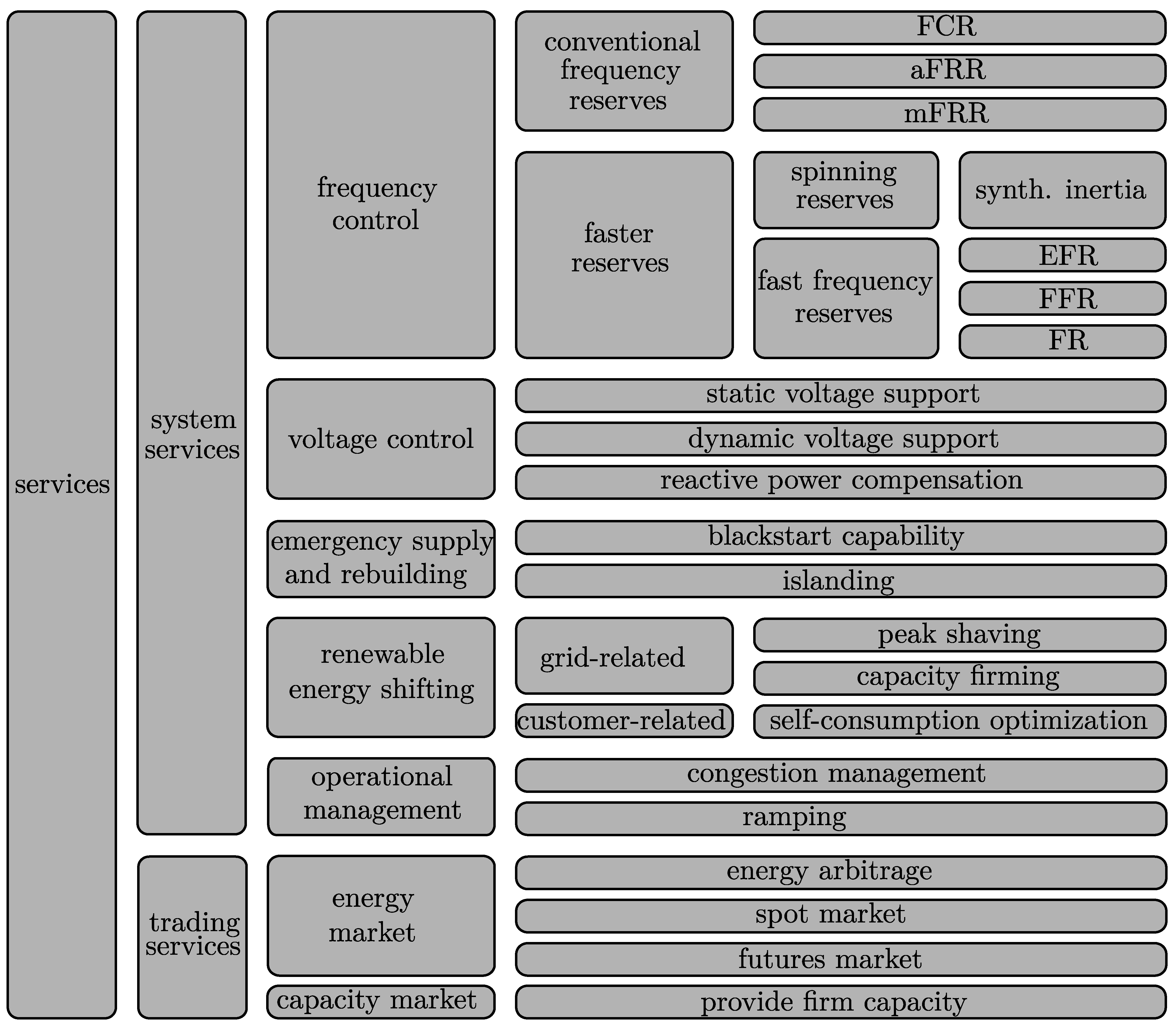
In order to reduce the greenhouse gas emissions, the European Union has defined the “Clean energy for all Europeans package”, which describes the corresponding measures up to 2030. These goals comprise an increase of the share of renewable energy by 32%, a reduction of the greenhouse gas emissions by 55% and an increase of energy efficiency by % by 2030, in each case compared to 1990. IRENA assumes the majority of renewable energy to be variable renewable energy such as wind power- and solar photovoltaic generation, which will represent 50% share of renewable energy in the power sector in 2030 [1]. This massive amount of variable renewable energy leads to increasing power fluctuations, which require additional flexibilities in the future power system. One way to provide such flexibilities are storage systems. Long- and short-term storage technologies therefore are expected to be increasingly integrated in the power system [2]. Battery Energy Storage Systems (BESS) are expected to cover a part of the short-term storage demand for durations between minutes, hours or days, especially due to their unique capability to quickly absorb, hold and then reinject electricity. IRENA estimates BESS to grow from a storage capacity of 11 GWh in 2017 to 100 GWh–412 GWh in 2030, which is expected to be evenly divided between front-of-the-meter (utility-scale) BESS and behind-the-meter BESS [3]. According to Hesse et al. [4], behind-the-meter BESS require a connection at the grid level of the meter and are typically integrated in the low-voltage- or medium-voltage grid, whereas utility-scale BESS typically are of larger size and integrated in the medium- or high-voltage grid. There are several services which are using the flexibility of a BESS and contribute to coping with power fluctuations in the future. Besides the prevention of curtailment of variable renewable energy, for example, by performing “peak-shaving”, which may aim to cache the energy surplus in times of high stress of the grid and release it in times of low stress of the grid, other services such as frequency control or voltage support are the main services currently provided by BESS [3]. Due to the moderate feed-in tariff for photovoltaic systems, the self-consumption optimization today is the most frequently used service for behind-the-meter BESS, which also contributes to destress the grid and to prevent curtailment. Based on the services identified in several studies [2,3,4,5,6], Figure 1 presents an overview of possible services BESS are suitable to provide.
Detailed descriptions of most of the services in Figure 1 can be found in literature [2,3,4,5,6]. Especially “faster reserves” according to Figure 1 are currently subject of intensive research activities [7,8,9,10,11,12,13,14,15]. Spinning reserve is inherently provided by conventional synchronous generators in the form of mechanical inertia, but may also be provided by inverter-based generation units in the form of “synthetic inertia” (SI) by adapting their control accordingly [16]. Fast frequency reserves, on the other hand, are activated identically to “frequency containment reserve” (FCR), namely based on the frequency deviation according to droop curves. There are various implementations, which are summarized under the term “fast frequency reserves”. Examples for actual products of such fast frequency reserves are the product “enhanced frequency response” (EFR), which has already been established in the United Kingdom [17], the product “fast frequency response” (FFR), which has already been established in Scandinavia [18], or the product “fast reserve” (FR), which will be established in Italy [19] shortly.
BESS have already become a promising provider of such services in recent years. The increase in the number of globally installed BESS from 200 in 2013 to 11 in 2019 underpins this statement [20]. However, in most cases, offering just a single service today is economically infeasible [21,22,23]. Providing multiple services, on the other hand, holds the potential for a more cost-effective operation of BESS and therefore is a hotly debated topic in literature [4,6,21,24,25,26,27,28,29]. However, such a multi-use operation, sometimes also referred to as multi-purpose operation or stacked operation, poses many challenges that must be considered for a successful realization.
One such challenge is the question as to which services are compatible when they are provided concurrently. According to EPRI, various aspects have to be considered in order to assess the compatibility of services that are associated with location-related, time-related and priority-related constraints of services [30]. For example, self-consumption optimization requires a location behind-the-meter, either on residential- or community scale. Time-related constraints refer to the feasibility of providing concurrent services. For example, that a service that requires discharging does not conflict with a service that requires charging or that providing one service now does not preclude another constraint service in the future (e.g., an acceptable range of state of charge—SoC for future applications). Constraints regarding prioritization of services refer to the circumstances in which certain services may have priority over other services. For example, the service of congestion management may provide power reserves during periods of peak infeed at a congestion point in order to store surplus power to prevent congestion or curtailment. Such a service demands power reserves regardless of wholesale market prices. Assuming congestion management to be valuable for system stability, it may have priority over services that are aiming at gaining revenues on the energy market, such as energy arbitrage or self-consumption optimization. During periods when a conflict of interest arises for such services, priorities are an option to handle their behavior. A report from Sandia National Laboratory [6] assesses the compatibility of services by technical- and operational compatibility. Whereas technical compatibility of several services is already given when the same BESS is capable of providing them, operational compatibility is determined based on operational conflicts that may arise due to location-related, time-related or priority related constraints as mentioned above. These operational conflicts are argued for different combinations of services throughout the report and are summarized in a “synergies matrix”, which evaluates the compatibility of couples of services based on the following categories: excellent, good, fair, poor and incompatible.
Besides such a general assessment of the compatibility of services, the most relevant challenges of a multi-use operation are its actual realization and implementation. Due to the limited power- and energy resources of a BESS, an allocation of certain power- and energy shares to services is necessary. Englberger et al. [24] identify three types of such an allocation, which are: sequential, parallel and dynamic. The sequential type is defined as an operation in which one service uses all resources of the BESS for a given time, after which another service takes over, etc. The parallel type is defined as an operation in which the resources of the BESS are divided in a predefined proportion between different services that are active at the same time. Shares of each resource can be viewed as “virtual BESS”, which provides a corresponding service and when put together forms the real BESS. The dynamic type is similar to the parallel type but dynamically allocates the share of resources for different time slots. However, as described by Namor et al. [25], a distinction must be made between an operational planning phase and a real-time operation. During the operational planning phase, the allocation of resources to services relies on the prediction of certain variables such as market prices or the power infeed of renewable generation. During the real-time phase, however, the allocation relies on variables that are measured in real-time.
Existing publications focus on the optimization problem of allocating resources of the BESS to different services via so-called “virtual BESS” in order to reach a certain optimization goal such as maximizing revenues [21,24,25,28,30,31]. In addition to such an operational planning, which is based on the results of such optimization models, the real-time behavior of a multi-use operation is a topic that has not been adequately addressed so far. Truong et al. [29], for example, describe an abstract definition of a multi-use operation and discuss possible issues during the real-time phase. They describe several conflicts of services during real-time operation and introduce the concept of priorities of services, which solves a conflict of services that leads to a total power exceeding the limits of the BESS. However, these descriptions only take into account active power and are only described on an abstract level. There appears to be a large gap to the actual implementation of a multi-use operation on real BESS that is capable of applying the results of an operational planning phase. In particular, the question of how to deal with unpredictable input variables in real-time operation has yet to be answered. This paper therefore tries to address the topic of the real-time multi-use operation of BESS in more detail. For this reason, this paper discusses concepts for implementing a real-time multi-use operation and introduces the novel concept of dynamic prioritization, which allows resolving conflicts of services. Besides the ability to cope with abnormal grid conditions during real-time operation, this concept also holds potential for a better utilization of resources during normal grid conditions.
A mathematical framework is presented that allows the definition of functions, which describe the execution of services and the description of the concurrent provision of services, taking into account the proposed concept of dynamic prioritization. For selected services, corresponding functions are described within this mathematical framework in order to demonstrate the functionality of the concept of dynamic prioritization in several applications. These applications include situations of normal and abnormal grid conditions. A model in Matlab/Simulink allows the simulation of these applications and demonstrates how the concept of dynamic prioritization can be used to cope with abnormal grid conditions. This model is also used to investigate a beneficial use of this concept during normal grid conditions in order to reach a better utilization of resources of the BESS. The corresponding application is investigated for a specific event and in the form of long-time simulations based on historical measurement data.
This paper is structured as follows. Section 2.1 presents possible concepts to realize a real-time multi-use operation of BESS. Section 2.1 discusses how to implement these concepts in a battery converter. Section 2.3 presents a mathematical framework to describe a multi-use operation of a BESS applying the concept of dynamic prioritization of functions, including the description of a corresponding current limitation in Section 2.3.1. Section 2.4 describes typical services provided by BESS via functions inside the mathematical framework. Section 3.1 presents several applications to demonstrate the behavior of the concept of dynamic prioritization and possible advantages over other concepts for a real-time multi-use operation. Section 3.2 discusses the results of a long-time simulation of one selected application. Section 4 concludes this paper.
2. Materials and Methods
2.1. Concepts of Real-Time Multi-Use Operation
In Section 1, three types of multi-use operation are described as sequential, parallel and dynamic, which were originally identified by Englberger et al. [24]. For all of these three types time-related constraints arise. As described in Section 1, there is existing literature on the consideration of these time-related constraints in optimization models, which allow the calculation of an optimal allocation of resources of the BESS for several services for each time slot in the optimization horizon regarding a specific optimization goal such as maximizing revenues. As described in Section 1, this phase is referred to as operational planning. The results of the operational planning can be used to parametrize corresponding schedules of services for each time slot in a real BESS accordingly. However, there are several services whose behavior is unpredictable during operational planning. This section discusses possible concepts to deal with such unpredictable behavior of services during real-time operation.
In this paper, the implementation of a service in a BESS is referred to as “function”. A service is considered as an abstract definition, whereas a function is a detailed definition of its implementation in a system. The implementation of a service as a function may differ between systems. Therefore, functions describe in detail how a service is executed. Besides such functions that are executing services, there may be additional functions that are necessary to operate a BESS or to guarantee the continuous execution of services. For example, the management of the state of charge (SoC) is one such function.
The first concept of real-time operation is based on a given allocation of virtual BESS for different services, which is the result of the operational planning for a specific time slot. The resources of a BESS can be split up into several virtual BESS. Such a division into virtual BESS has to be done for the power resources and the energy resources of the BESS, resulting in corresponding power bands and energy bands that represent the share of resources of each virtual BESS related to the total resources of the BESS. However, there is a difference between power bands and energy bands in the way they are influenced during real-time operation. While the power band of a virtual BESS defines the limits within which the operating point of an assigned function is allowed to operate, the energy band of a virtual BESS defines the reservation of energy resources of the BESS for a later usage by the corresponding function.
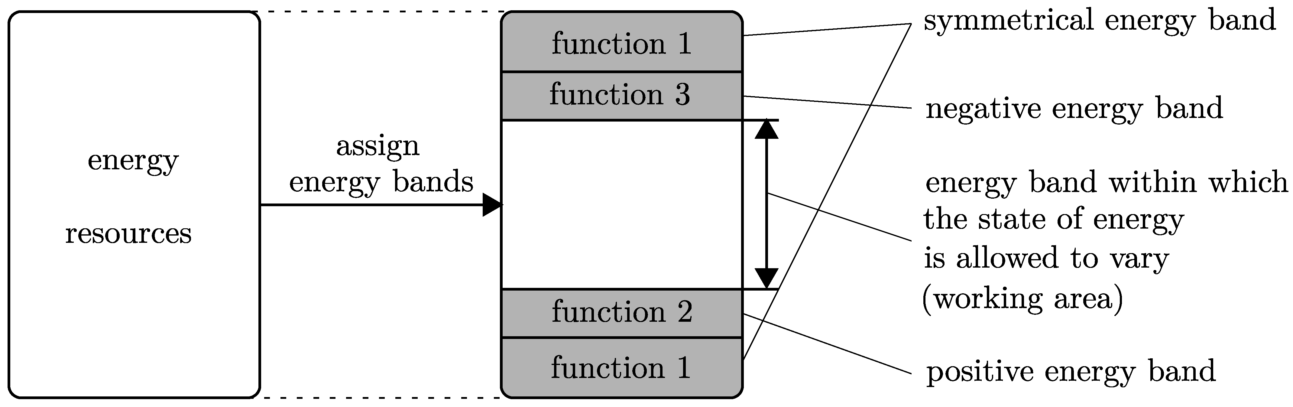
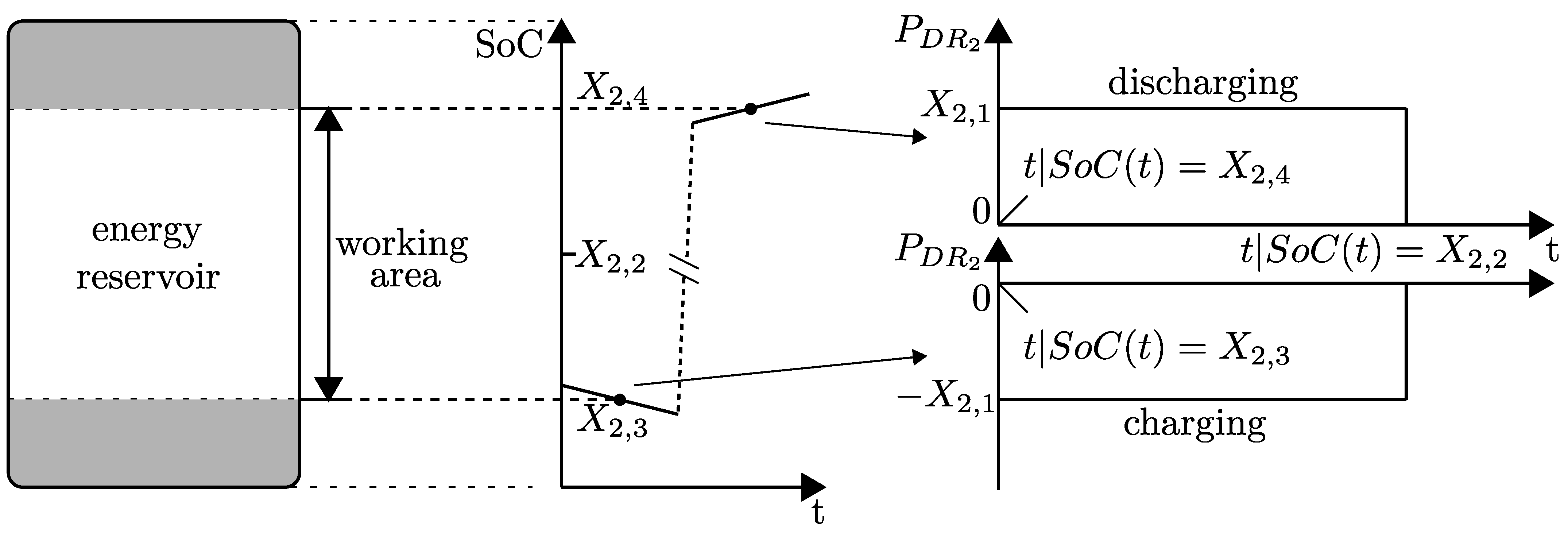
Figure 2 illustrates the first concept of real-time multi-use operation based on the allocated energy bands for each function in a specific time slot. A BESS that executes four services is assumed. Since the state of energy is a state variable it has an influence in which way the energy band of the corresponding virtual BESS is allocated within the energy resources of the BESS. The energy bands can either be allocated symmetrically, positively or negatively. In the case of symmetrical allocation, the energy resources of the corresponding virtual BESS are allocated with half their value in the upper and lower region of the energy resources. In case of positive allocation the energy resources of the corresponding virtual BESS are allocated in the lower region of the energy resources. In case of negative allocation, the energy resources of the corresponding virtual BESS are allocated in the upper region of the energy resources. A symmetrical allocation ensures that the BESS can store and provide energy at a later point in time, while a positive allocation only ensures the provision and a negative allocation only ensures the storage at a later point in time. As described in [32], an example of a service that requires symmetrical allocation is FCR. An example of a service that requires negative allocation is peak shaving. Peak shaving requires specific negative energy resources to be available in advance of its activation in order to be able to store energy while it is active. An example for positive allocation is the provision of firm capacity. Providing firm capacity requires specific positive energy resources to be available in advance of its activation in order to be able to provide energy while it is active. Furthermore, there are functions whose requirement for an energy band is zero. All voltage control services are of such type. Figure 2 shows a symmetrical allocation for function 1, a positive allocation for function 2, a negative allocation for function 3 and no energy band for function 4 in order to illustrate the resulting energy band, the so-called “working area”, within which the state of energy of the BESS is allowed to operate.
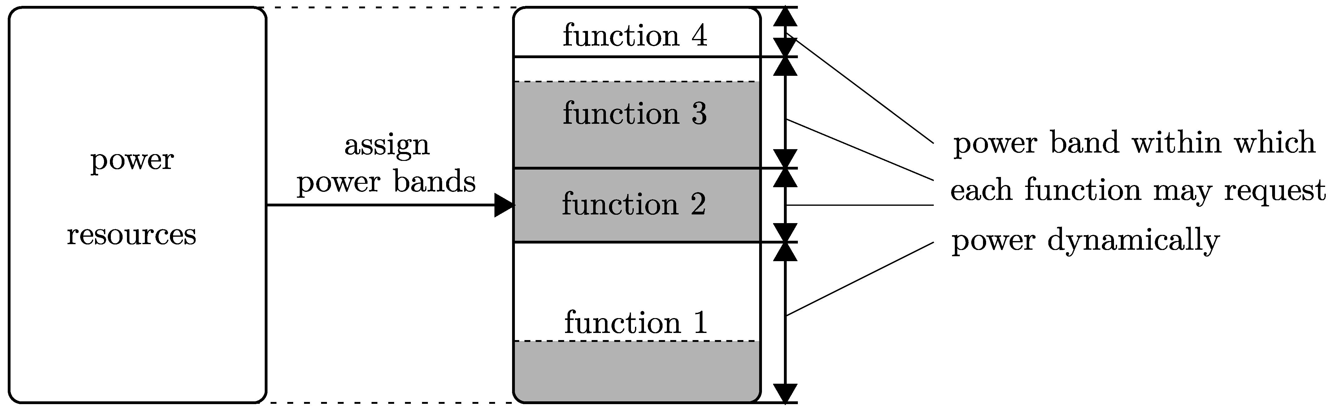
Figure 3 illustrates the first concept of real-time multi-use operation based on the allocated power bands for each function in a specific time slot. A BESS that executes four services simultaneously is assumed, where function 1 and function 3 are only partly exploiting their power band, whereas function 2 fully exploits its power band and function 4 does not have any power output. Conflicts of functions are avoided on the basis of such a concept. Since power resources are divided in advance to the actual real-time operation, the sum of the power output of all functions cannot exceed the power resources of the BESS.
However, most of the unpredictable services require large amounts of power resources only during rare events such as abnormal grid conditions. On the one hand, these power resources have to be reserved in corresponding virtual BESS at all times, but on the other hand, this reduces the flexibility for other services. With regard to Figure 3, such a situation may arise when function 1 and function 4 are assumed to be functions that execute such unpredictable services. Most of the time their request of power resources is small compared to the size of the allocated virtual BESS. The flexibility to allocate resources for function 2 and function 3 during operational planning therefore is limited, although a high share of the resources is unused most of the time.
The question arises as to whether there are services that are capable of using the same resources and whether there are situations when the concept of virtual BESS needs to be expanded. Sharing energy bands is not possible, but sharing power bands is an option. For example, different services for frequency control may be considered as decoupled in time to some extent and may be candidates to use shared power bands. Furthermore, there are services whose provision quality is not affected by the short-term sharing of power bands. As will be shown in Section 3.1, static voltage support can be considered as such a service. Besides the argument of better utilization of resources, there are services whose resource demand cannot be identified in advance and which may require the concept of allocation of virtual BESS to be overruled in order to contribute to system stabilization. As will be shown in Section 3.1, dynamic voltage support can be considered as such a service. All of these thoughts are considered in the next concept, which is described below.
The concept of dynamic prioritization is also based on the allocation of virtual BESS and allocates energy bands identical as shown in Figure 2. However, regarding power bands, an allocation is only done for functions for which such an allocation is possible. Based on priorities, the power resources of virtual BESS for functions with lower priority are made available for functions with higher priority when required. With such an approach it is possible to deal with the unpredictable behavior of services in such a way that during abnormal grid conditions they can exploit the corresponding resources but at the same time do not waste resources through corresponding reservations during normal grid conditions.
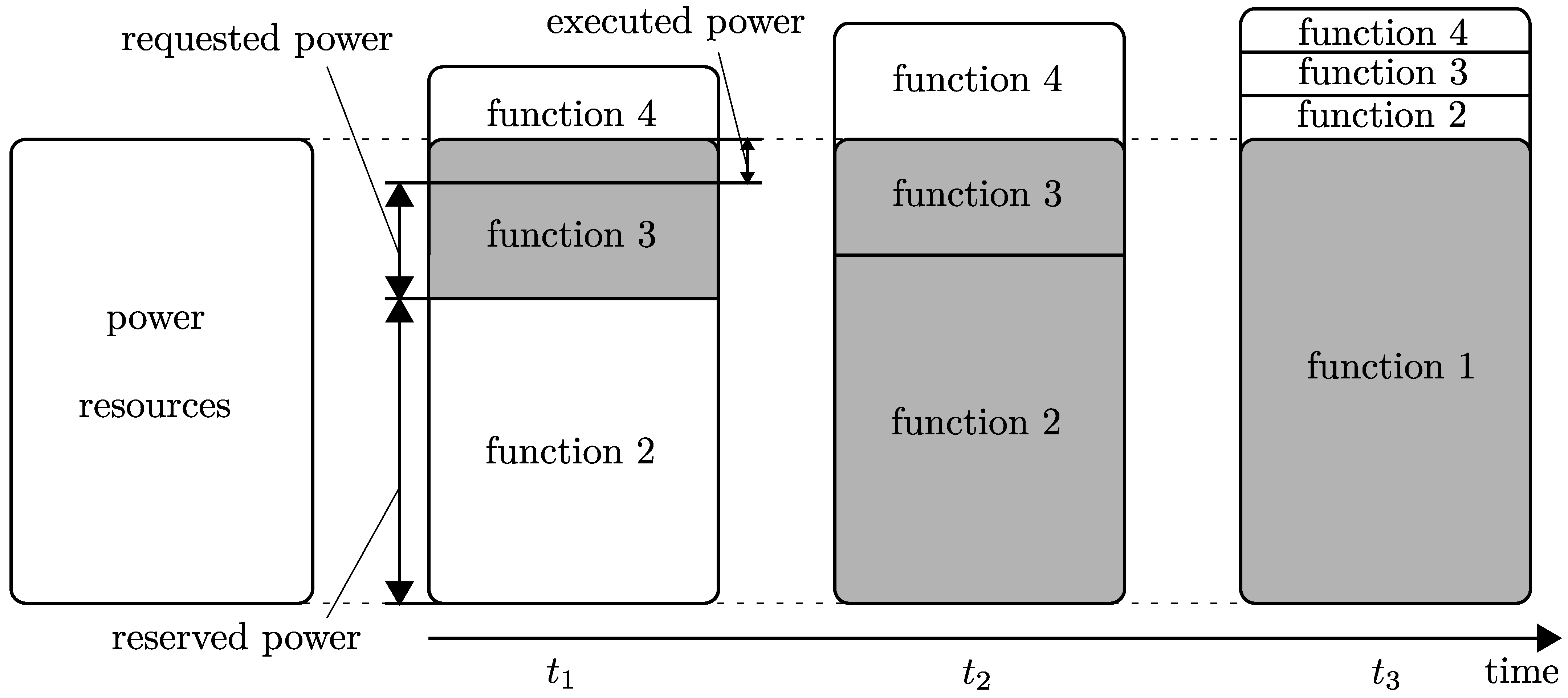
Figure 4 illustrates this concept of dynamic prioritization, again assuming a BESS providing four functions.
Priorities are assigned beginning with function 1, which is assigned the highest priority, up to function 4, which is assigned the lowest priority. In this example a virtual BESS with a corresponding power band is assigned only to function 2, which ensures the reservation of certain power resources of the BESS. In order to describe the behavior of functions in this concept, it is distinguished between
- reserved power: power resources according to the size of the virtual BESS assigned to the corresponding function,
- requested power: real-time power demand of the function and
- executed power: power output the system is able to execute for the corresponding function.
An activated function is allowed to reserve-, request- and execute powers, whereas a deactivated function is not allowed to do so. A function is active only when its executed power differs from zero, otherwise the function is inactive.
Figure 4 shows three different situations at the time , and , where the four functions are activated and have different requested powers for each situation. At the time function 1 and function 2 are inactive. However, for function 2 power resources are reserved according to the size of the allocated virtual BESS. Function 3 and function 4 are active and are using the remaining power resources. However, since the requested powers of all functions exceed the power resources there is a conflict of functions, which is resolved based on the priorities. Since function 3 has a higher priority than function 4, the requested power of function 3 can be fully executed, whereas the requested power output of function 4 is limited, leading to an executed power that is lower than the requested power. At the time function 2 fully exploits its allocated power resources and even requests a higher amount than reserved according to its virtual BESS. Due to the priorities, the power requests of function 4 cannot be executed any more and the function becomes inactive. At the time it is assumed that an abnormal grid condition leads to a power request of function 1 that fully exploits the whole power resources of the system. Due to the highest priority of function 1, requested powers of all other functions cannot be executed any more and power reservations are overruled. Therefore, the functions 2–4 become inactive.
Compared to the concept of virtual BESS of Figure 3, which prevents the occurrence of conflict of functions, the concept of dynamic prioritization of Figure 4 handles conflicts based on the priorities assigned to each function.
At the times and the whole power resources of the BESS are exploited. Assuming an immediate transition between these two situations, the question arises as to what influence the different assignments of power resources have, since the total power output of the system does not seem to change. The description of concepts in this section is based on a one-dimensional view. For example, it is not distinguished between active- and reactive power. Assuming the function 2 and function 3 to request active power and function 1 to request reactive power in Figure 4, the change of the total power output between the time and becomes visible. There are several other dimensions that have to be considered during the multi-use operation. Besides the active- and reactive power, for example, the influence of asymmetry and harmonics has to be taken into account. With consideration of such additional dimensions, a change of assignments at the time and in Figure 4 therefore has an influence on the total power output of the system, since the waveform may change depending on the functions that are active. The sign of the power is an additional matter that is not considered in the exemplary descriptions above.
2.2. Considerations on the Realization in Battery Converters
The descriptions of concepts in Section 2.1 are based on the assumption of a limited power capability of a BESS. To describe concepts, this assumption is helpful, because it allows a simplified description, but in more detail this limited power capability goes back on the maximum current a BESS is capable of handling, which is limited by its converter. This maximum instantaneous current , therefore, is the ultimate value, which has to be considered in the converter control. As already described at the end of Section 2.1 there are several dimensions that have to be taken into account when assigning power resources to different functions. Compared to the one-dimensional examples described in Section 2.1, the realization of a multi-use operation in a converter control structure requires a multi-dimensional assignment of resources. A typical converter control structure, such as described in [33], consists of a power control and a current control. Active- and reactive power set points are used to calculate current set points, which are typically described by a normalized current space vector . The nomenclature used in the following descriptions is summarized in Nomenclature. A summarized list of all symbols used in this paper can be found in Appendix B.
An assignment of resources has to ensure the condition
at any time. Therefore, an extended version of the concept described in Figure 4 has to be applied, which takes into account the multi-dimensional character of the current space vector .
Such an extended version of the concept of Figure 4 is described in Section 2.3. Based on a mathematical framework, which allows the definition of functions, the description of their behavior regarding requested powers and the formulation of a dynamic prioritization of functions based on priorities, a systematic description of a real-time multi-use operation of BESS is possible.
2.3. Mathematical Framework to Describe a Multi-Use Operation
The multi-use operation is based on a set of functions
where each function , with describes the behavior of the corresponding service the BESS provides. The number of functions is . A function is either activated or deactivated. This activation of functions is described by the set
with , and where means the function is deactivated, and where means the function is activated. There may be functions that must not be activated at the same time because they are incompatible. These forbidden activations are summarized in the set
According to Section 2.1 it is distinguished between the reserved-, the requested- and the executed power. Each function describes the behavior of its requested power, based on a set of parameters
where is the number of parameters of the function and a set of control variables
where is the number of control variables of the function . Based on these parameters and control variables the behavior of the requested power of each function can be described. The requested power is divided into two parts, a statically requested part and a dynamically requested part. The statically requested power represents the static operating point, whereas the dynamically requested power represents the dynamic behavior of the power output that follows this operating point. The statically requested power of a function is defined by
and the dynamically requested power of the function results from the dynamic behavior, defined in the parameters of the function, and the statically requested power
Both the statically- as well as the dynamically requested part are apparent powers, which consist of an active- and a reactive power, which are and for the statically requested power and and for the dynamically requested power.
Many functions only request either active- or reactive power. The two sets and therefore are defined by
and include the corresponding functions that only request active- or reactive power. All functions included in the set are called “active power functions” and all functions included in the set are called “reactive power functions”.
As described in Section 2.2 the converter control structure typically includes the inverter current control, whose input are four Park-components, which are summarized in the vector
The contribution of each function to has to be calculated based on the dynamically requested power on the basis of the corresponding current request:
Besides the requested power, Section 2.1 lists the reservation of power resources in order to ensure that functions are capable of executing certain power increments at any time. Such a power reservation of a function results in a corresponding reservation of current reserves in the “power control” of Figure 4, which is defined by
and reserves either positive-, negative- or symmetrical power resources. For example, FCR requires a symmetrical reservation of power resources, whereas for aFRR it is possible to tender positive- and negative products separately.
In Section 2.1 a conflict of functions was indirectly defined as a situation where a function requests power but is prohibited to execute it. With regard to the corresponding current request , such a situation is characterized by a limitation of . Therefore, the different current contributions of functions sum up to
where the executable current request of each function is . This executable current request is defined by
and depends on the requested current and the already “occupied current capabilities” of functions with higher priority than the function , which will be defined in Equation (23).
In case of a conflict of functions, at least one current request of a function has to be limited, which leads to
To manage such a conflict of functions a set of priorities is defined by
Each function is assigned a priority according to
A function has highest priority when and it has lowest priority when . When a conflict of function occurs, the current requests of functions are limited, beginning from the function with lowest priority , up to the function with highest priority , until the condition according to Equation (1) is fulfilled. In order to identify the functions which have to be limited, a set is defined for each function , which consists of all function indices with higher priorities than . These sets are defined by
In order to calculate the limited currents for each function in case of a conflict of functions, a matrix is defined by
which describes the already “occupied” current resources considered from the point of view of function and where the value of m is depending on the number of current requests, which exceed the current reservation of the corresponding function. In case there are no current reservations, this leads to . In case of at least one function with higher priority reserving current resources symmetrically and assuming all current requests are zero, this leads to , since every symmetrical current reservation has to be taken into account with positive- and negative sign. In order to realize a behavior as shown in Figure 4 the occupied current resources for each function are depending on the current requests and current reservations of all functions with higher priority than . Since each function may have positive-, negative- or symmetrical current reservations and may be an active- or reactive power function, this leads to a rather complex structure of Equation (21). The first part of the case distinction in Equation (21) takes into account a situation when a current request exceeds current reservations but also comes into force when a function has no current reservation. For example, a current request with a corresponding current reservation and a current request has to result in executable currents of and when and . However, current reservations only have to be taken into account for the corresponding type of function. For example, for an active power function only current reservations of other active power functions with higher priority have to be taken into account, whereas current reservations of reactive power functions do not have to be taken into account. Such a behavior is described by the second and third part of the case distinction in Equation (21).
Each column vector in can be assigned a maximum phase current that would occur in one of the three phases, in case the corresponding vector would be executed. The set of these maximum currents where each entry is the maximum phase current of the corresponding column vector out of is defined by
where is the angle between the positive- and negative-sequence system. In this set of maximum phase currents , a maximum can be found, which is assigned to the corresponding vector. This corresponding vector that leads to this maximum phase current is defined by
The maximum phase current and its corresponding vector can be used to calculate the executable currents of each function by
where the lower part of the equation corresponds to Equation (16) and leads to a current limitation of the current request of function . A detailed description of the calculation of this current limitation of Equation (24) is described in Section 2.3.1.
Calculation of Limited Currents
Any current space vector in the -plane is a function of its Park-components, the grid angle and the angle between positive- and negative-sequence system:
Assuming there is no zero-sequence system, the relationship between a current space vector in the -plane and a current space vector in the -plane is given by the Park-transformation
In more detail, a current space vector can be expressed by
where a division of the space vector in a positive-sequence part and a negative-sequence part is considered. Each of these two parts can be further divided into a direct- and a quadrature part by using
All four Park-components can be summarized in a vector . The instantaneous phase currents can be calculated by projecting the space vector on the corresponding phase:
To calculate the maximum phase current, the corresponding grid angle , which is calculated by
can be used as follows
Equation (32) can be used to calculate the individual maximum phase currents in Equation (22):
which leads to the maximum phase current
in Equation (23).
When a current limitation according to the lower part in Equation (24) is necessary, a procedure has to be defined, that determines which of the four components of the corresponding current request of a function have to be limited and to what value they have to be limited. In Equation (24) this procedure is represented by the term . In order to describe this term in more detail all functions that need to be limited have to be identified first. The case distinction in Equation (24) implicitly reveals all functions that have to be limited. According to Equation (24), all functions with the function index k out of the following set
have to be limited. In this set , the function with highest priority can execute a limited amount of its current request, whereas the current request of all other functions have to be limited to zero. This function is defined by
For this function , the limited currents have to be calculated explicitly, whereas for all other functions , the corresponding executable currents according to Equation (24) are zero:
For the calculation of of the function , a stepwise approach as described in [33] can be applied under the use of , where consists of fixed values of executable currents of functions with higher priority than the function and is to be calculated by the current limitation algorithm described in [33]. In a first step, a prioritization of the direct- or quadrature components of the function has to be defined. For the sake of simplicity, this prioritization is assumed for the quadrature components, identical as in [33]. Furthermore, it is assumed that the -component is zero. Taking into account these assumptions, the three remaining components , and can be calculated according to the Algorithm described in [33].
2.4. Description of Selected Functions
Based on the services shown in Figure 1, selected functions are presented in this Section, which are described within the mathematical framework of Section 2.3 and which are taken into account in Section 3. The selection of functions is based on the capabilities of a real BESS system, which is described in more detail in [32], as well as on their suitability to describe applications in order to demonstrate the concept of dynamic prioritization. Table 1 gives an overview of these functions. Each of the functions is assigned a function index according to Equation (2).
Section 2.4.1 presents a detailed description of the function based on the framework of Section 2.3 in order to demonstrate the application of the framework to describe functions. Such detailed descriptions for the remaining functions out of Table 1, on the other hand, are given in Appendix A.
2.4.1. FCR
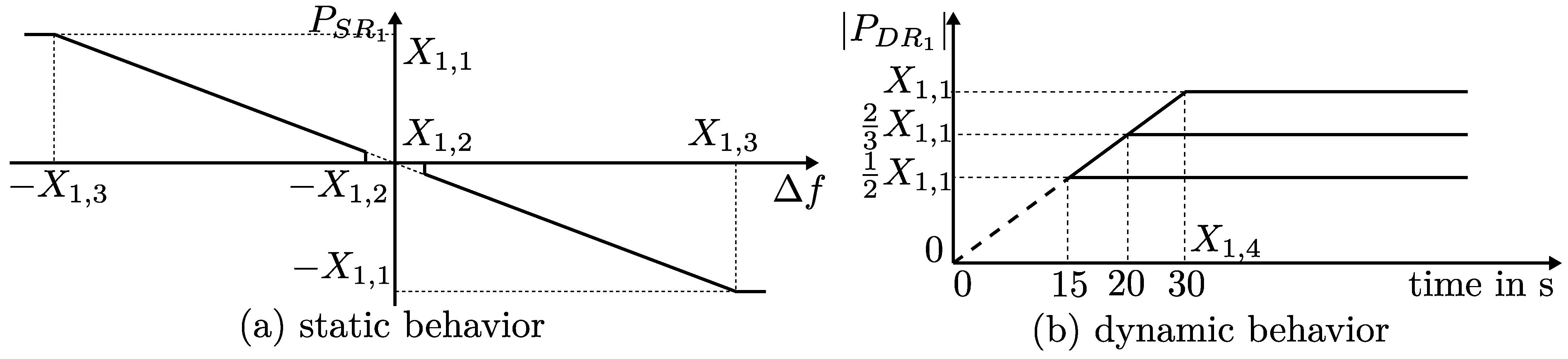
FCR is the first stage of the conventional load-frequency control. Following a difference between load and generation in the electric power grid, a frequency deviation in relation to the nominal frequency occurs. All technical entities which are providing FCR are taking part in stabilizing the grid frequency according to a droop control. According to the system operation guideline (SOGL) [34], which defines the regulatory requirements for FCR in Continental Europe, a full activation of FCR takes place in the case of a frequency deviation of 200 . A full activation equals a power output of the technical entity, which is identical to the corresponding tendered FCR-power. The full activation time after which such a full activation has to be reached is 30 following the occurrence of a frequency deviation. These requirements are illustrated in Figure 5, where the frequency deviation is calculated by
In accordance with Section 2.3, the corresponding statically- and dynamically requested powers of the function can be defined by
and
The parameter defines a frequency deadband, which represents an insensitivity area that takes into account possible frequency measurement errors and which is usually defined with 10 . All parameters of the function are summarized in Table 2.
Although most of the parameters in are prescribed by SOGL [34], there are cases where some of them may be altered. For example, it may be an option to dynamically adapt the parameters dependent on the SoC in order to contribute to SoC-management, as described in [32].
According to Section 2.3 the corresponding current request of function has to be calculated based on the dynamically requested power. The current request can be calculated by
The control variables of function therefore can be summarized to . Assuming and nominal frequency , a power increment with a value of should be possible all the time. Therefore, a corresponding current reservation according to Section 2.3 has to be done. This current reservation can be calculated by
in accordance with Equation (13).
2.4.2. SoC-Management
Due to the limited energy reservoir of a BESS, a suitable SoC-management is essential. The SoC-management implements does not implement a corresponding service but ensures that other services can be offered continuously. The basic concept for handling energy resources has already been described in Section 2.1. This function implements the behavior described in Figure 2, which shows an energy band within which the state of energy is allowed during real-time operation. The state of energy is directly related to the state of charge. However, during real-time operation usually the state of charge is used. The energy bands of Figure 2 can be transformed into corresponding SoC-bands. The consideration of each SoC-band leads to an area within which the actual SoC is allowed to operate, which is termed as “working area” of the SoC. This function therefore ensures that the actual SoC is kept within this working area. When the actual SoC of the BESS reaches the corresponding limits of such SoC-bands, a charging- or discharging action is initiated.
A detailed description of the function based on the framework of Section 2.3 is given in Appendix A.1.
2.4.3. FR
FR is one possibility to offer a service which acts as faster control reserve. FR basically has a similar behavior as FCR, but its full activation time is much shorter, compared to the full activation time of FCR. Furthermore, its duration of activation is limited, whereas the duration of activation of FCR generally is not limited.
A detailed description of the function based on the framework of Section 2.3 is given in Appendix A.2.
2.4.4. SI
SI can be described as imitation of the behavior of mechanical inertia in converter-based systems. A detailed description of possible implementations of SI is given in [16].
A detailed description of the function based on the framework of Section 2.3 is given in Appendix A.3.
2.4.5. Static Voltage Support
Many grid codes, for example [35] in Austria and [36] in Germany, require inverter-based generators to provide static voltage support. This is achieved by certain reactive power consumption or reactive power infeed, depending on the actual voltage in the grid. The reactive power influences the local grid voltage and can therefore be actively controlled in order to support the voltage maintenance in the grid.
A detailed description of the function based on the framework of Section 2.3 is given in Appendix A.4.
2.4.6. Dynamic Voltage Support
Besides the static voltage support, many grid codes also require inverter-based generators to provide dynamic voltage support. Similar to static voltage support, dynamic voltage support is achieved by reactive power injection or consumption. While static voltage support is used for contributing to voltage maintenance during normal grid conditions, dynamic voltage support becomes active only during grid faults, for example, short-circuits, to dynamically stabilize the voltage during such conditions. The prescriptions in grid codes, for example in [35,36], require a certain reactive current increment in response to the voltage drop during short-circuits.
A detailed description of the function based on the framework of Section 2.3 is given in Appendix A.6.
2.4.7. Island Operation
All foregoing functions rely on a converter control structure which is referred to as “grid-following” control approach. A grid-following control approach is based on a measurement of the grid angle . Therefore, such an approach is only feasible in case there are other generating units in the grid as well. In case of a Microgrid, on the other hand, where a BESS is the only generating unit, a so called “grid-forming” control approach has to be applied instead of a grid-following approach. With a grid-forming control approach, the grid angle is generated by the converter itself instead of measuring it based on the grid voltage. An island operation therefore requires the implementation of such a grid-forming control approach. This makes the function , which describes the island operation in this paper, the only function out of the list in Table 1 which requires the control structure to be changed. A description of how to achieve such a change of the control approach from grid-following to grid-forming, for example, is illustrated in [16].
A detailed description of the function based on the framework of Section 2.3 is given in Appendix A.6.
3. Results and Discussion
This section is divided into two parts. Section 3.1 investigates selected applications during specific events via short-term simulations, while Section 3.2 investigates one of these applications in a long-time simulation. A real BESS system, which is described in more detail in [32], is used as the basis for parametrization of the simulation models.
3.1. Selected Applications to Demonstrate the Use of Dynamic Prioritization
The mathematical framework presented in Section 2.3 introduces the set of activations , the set of priorities and the sets of parameters for each function . Compared to the sets of control variables of each function , which are also introduced in Section 2.3, , and have to be parametrized in advance to a real-time operation, whereas the control variables are measured during real-time operation.
With regard to Section 1, the operational planning phase results in the parametrization of , and for each time slot of the planning horizon. This determination takes place a predefined time before the real-time operation, e.g., one day ahead.
Section 2.1 mentions the difficulties of unpredictable services to be considered in the operational planning phase. Considering the services whose execution is described via functions listed in Table 1, these difficulties can be discussed in more detail. Examples for such unpredictable services are services for frequency control. Three functions for frequency control are considered in Table 1. However, while the executed powers for all of these functions are unpredictable during the operational planning phase, for the functions FCR and FR at least a corresponding reservation of resources can be considered in the form of virtual BESS. For the service SI, on the other hand, its definition in Appendix A.3 allows the request of the full power resources of the BESS, ignoring the borders of allocated virtual BESS. In the rare event of the occurrence of very high frequency gradients, such a situation may happen. Therefore, two categories of unpredictability of functions can be identified, which are
- (a)
- unpredictability regarding execution inside a virtual BESS and
- (b)
- unpredictability regarding the request of resources.
Such an unpredictability type can be assigned to all functions from Table 1. The results for such an assignment are summarized in Table 3.
Besides the function SI, Table 3 lists Dynamic Voltage Support and Island Operation to be from unpredictability type (b). Both functions may request the full power resources of the BESS in case of a short-circuit (Dynamic Voltage Support), or in case of a blackout of the power system (Island Operation). Due to the definition of the function Static Voltage Support in Appendix A.4 this function can be considered as perfectly predictable, since it requests a predefined amount of resources at any time. With regard to Figure 1 there are several other services which can be considered as perfectly predictable, such as energy arbitrage or providing firm capacity.
Since functions of unpredictability type (b) cannot be considered during the operational planning phase by allocating virtual BESS, an appropriate concept of how to react during real-time operation in case of rare events during abnormal grid conditions, where corresponding functions may exploit the full power resources, is necessary. The concept of dynamic prioritization presented in Section 2.3 is capable of handling such events. One goal in this section therefore is to demonstrate the behavior of the concept of dynamic prioritization during such events based on the functions described in Section 2.4. Section 3.1.1 and Section 3.1.2 describe corresponding applications.
Section 2.1 describes functions of unpredictability type (a) to diminish flexibilities for other functions. The allocation of virtual BESS for such functions during the operational planning phase leads to the reservation of relatively large amounts of resources, which are fully utilized only in the case of infrequent events during real-time operation. The concept of dynamic prioritization presented in Section 2.3 allows a better utilization of the reserved resources from functions of unpredictability type (a). A second goal in this section therefore is to demonstrate how the concept of dynamic prioritization can be used to achieve such a better utilization of resources during normal grid conditions based on the functions described in Section 2.4. Section 3.1.3 describes a corresponding application.
The operational planning phase may result in different priorities of functions between time slots. However, based on the functions which are listed in Table 1, a meaningful static assignment of priorities can be argued, which is used in order to describe the applications in this section. The highest priority is assigned to function , island operation, with . Although it has already been stated in Appendix A.6 that a combined activation of another function together with is not allowed (), according to Equation (18) a priority has to be assigned to all functions, because . The next higher priority is assigned to function , dynamic voltage support, with . When the function becomes active, it contributes to solve a local- and dynamic voltage problem. Since a long duration of such a voltage problem may lead to the trip of protection relays in the feeder the BESS is connected to, the prevention of such a situation has high priority. Since fault conditions in the grid typically only last for short time periods until the fault is cleared (e.g., several seconds), the possible limitation of other functions by may not be considerable, for example regarding revenues. In addition, the function only provides reactive power, and therefore does not influence the SoC. The next higher priority is assigned to function , SoC-Management, with . Since the function ensures an appropriate energy reservoir at any time, which is necessary for a continuous provision of services, its priority is relatively high. Although functions as , FR, and , SI, are little energy intensive and are only active during short durations, a possible current reservation by these functions may lead to a longer lasting limitation of the function , SoC-Management, when they are assigned higher priority than has. In order to prioritize current requests of over current reservations of other functions, the priority of is higher than the priorities of the remaining functions. The next higher priorities are assigned to the functions , VI, , FR and , FCR, with , and . Since all of these three functions are contributing to the global stabilization of the frequency in the grid, which is one of the most relevant services in the electric power system, their priorities are relatively high. The function has higher priority , because the clearance of a local dynamic voltage problem is considered to be more important than the global frequency stabilization. The assignment of priorities between the three functions is discussed in more detail in Section 3.1.2. The lowest priority is assigned to function , static voltage support, with . Since the contribution to static voltage support can be considered as long-term goal, a possible limitation by other functions may not be a problem as long as the function can be temporarily active between times of short-time limitations.
For all applications it is assumed that a BESS with an apparent power of is offering the corresponding services of the functions of Table 1 with an assignment of priorities as described above: . Furthermore, a nominal frequency of and a maximum current capability of and are assumed.
3.1.1. Application 1: Occurrence of Grid Faults
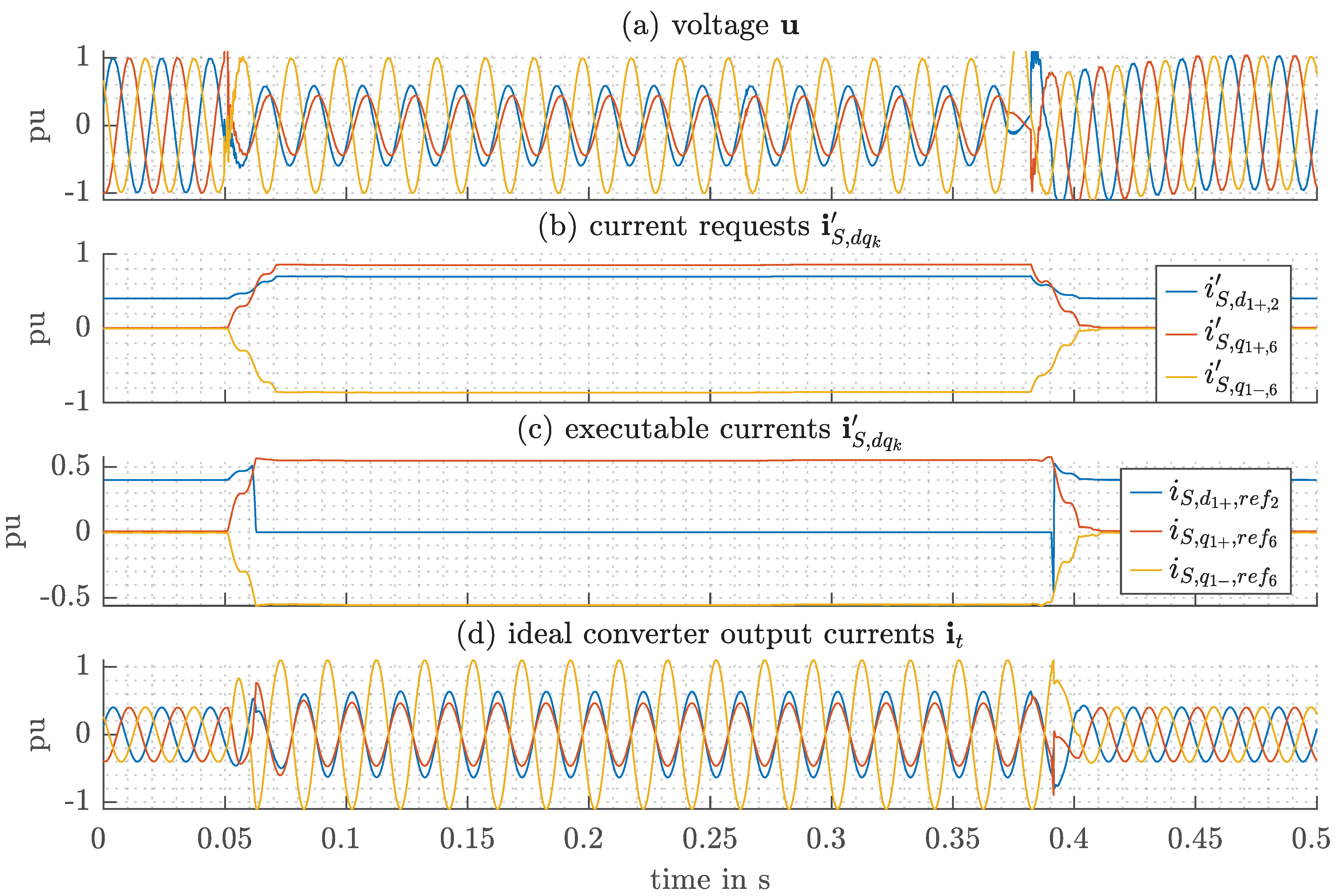
A short-circuit event can be viewed as an abnormal grid condition that cannot be predicted in the scope of the operational planning phase. During short-circuit events in the grid, the function , Dynamic Voltage Support, becomes active in order to dynamically stabilize the grid voltage. At the moment of occurrence of the short-circuit, other functions of the BESS may be active already. Due to the high priority of the function , its current request is prioritized over the current requests of other functions. Figure 6a shows the normalized phase-to-phase voltages during a two-phase short-circuit nearby the point of common coupling of the BESS, which were measured in the scope of [37]. The two-phase short-circuit leads to a drop in the positive-sequence voltage and a rise in the negative-sequence voltage . According to Appendix A.5 this leads to current requests of the function . Assuming the functions and to be the only activated functions and also assuming the function , SoC-Management, to be active before, during and after the short-circuit, this leads to a conflict of functions. It is assumed that and , which corresponds to . Figure 6b shows the corresponding current requests of the functions and . Because of the drop of during the short-circuit, the current request of rises according to Equation (A3). Figure 6c shows the corresponding executable currents. The current requests of the function are and , which lead to a conflict of functions in combination with the current request of the function , which is . Due to the higher priority of in relation to , with , the executable current of during the short-circuit is . According to Section 2.3.1, also the current requests of have to be limited to respect the maximum current capability. Figure 6d shows the corresponding phase currents, which result from the executable currents.
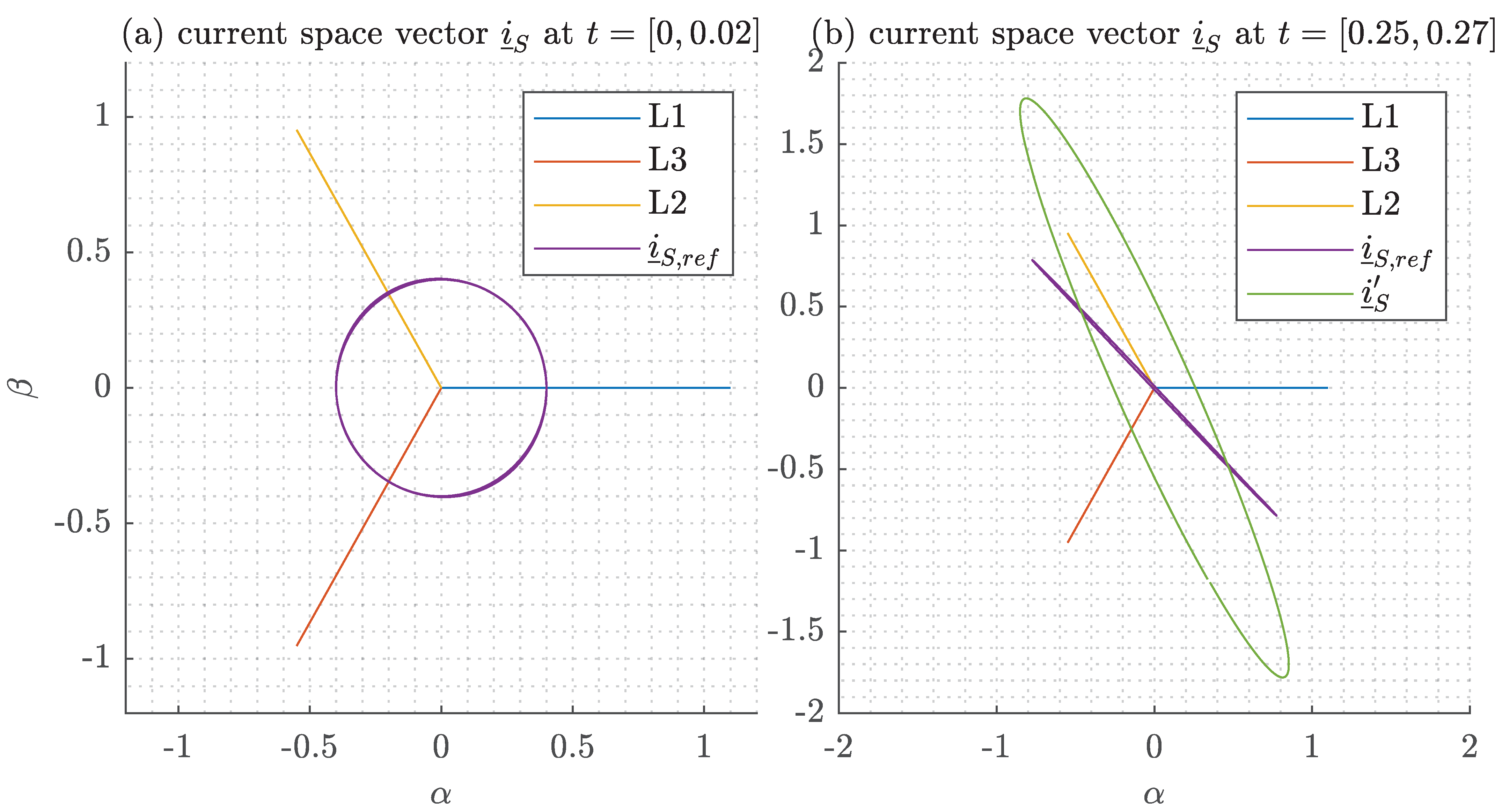
Figure 7 shows the corresponding vector diagrams in the -plane before and during the short-circuit event. Figure 7b shows that the execution of the requested current space vector would exceed the current capability of . The current limitation leads to a corresponding executable current space vector . Figure 6c and Figure 7b both show that the maximum current capability of is respected by this executable current space vector .
With regard to Figure 3 and Figure 4, a comparison of the corresponding concepts of static power band assignment and dynamic prioritization can be made. Assuming a situation as described above and applying the concept of static power band assignment according to Figure 3, this would make it necessary to predefine power bands for the function and . This would lead to a different behavior in Figure 6c,d, where the output of function would remain constant and the reactive current contributions of would be lower. The result would be a less effective influence on the dynamic voltage stabilization during the short-circuit. Applying the concept of dynamic prioritization, on the other hand, allows the function to fully exploit the current capability of the BESS, without the necessity to share the power capability between and .
3.1.2. Application 2: Simultaneous Provision of Frequency Reserves
With SI, FFR and FCR, three frequency control services have already been discussed in this paper. These services act in different time horizons. Whereas SI acts fastest in response to a frequency deviation, it is followed by FR and FCR, the latter acting slowest among the three services. Although the three services interact during activation, they can approximately be viewed as decoupled in time. Such a view opens up the possibility of providing all services based on the same power reserves without having to allocate reservations for each service. The tendering of the same amount of power reserves for different kind of frequency control services may be forbidden due to legal requirements. However, new services as FR are still under discussion; therefore, such a possibility of concurrent provision is assumed in the following.
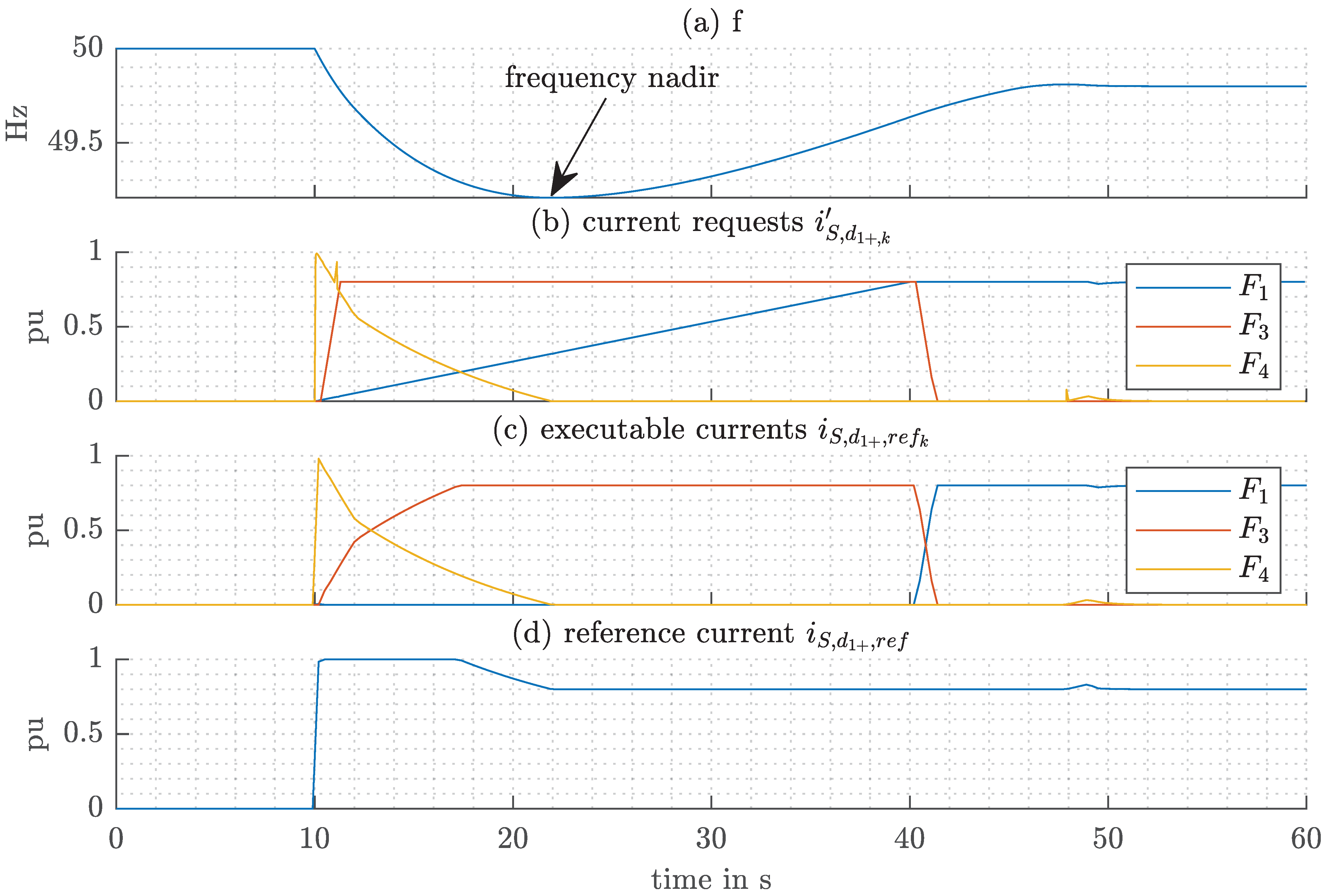
All three services become active during frequency deviations. A so-called “reference incident” [38] is assumed to lead to the worst-case frequency deviation curve in Continental Europe. It assumes the failure of two major power plants with a corresponding power of 3 , leading to a frequency deviation curve as shown in Figure 8a. This reference incident is considered to discuss the simultaneous provision of the three frequency control reserves mentioned above, while applying dynamic prioritization of functions. It is assumed that the functions , FCR, , FR, and , SI, are the only activated functions with and are parametrized as follows. For the function , FCR, the tendered FCR-power is , which corresponds to . For the function , FR, the tendered EFR-power is , which corresponds to . For the function , SI, the parameters are and and a static current reservation of is parametrized. The positive-sequence voltage is assumed to be constant .
Figure 8b shows the corresponding current requests of the functions in response to a reference incident. In order to respect the current reservation of , SI, and the maximum current capability of , the executable currents are calculated according to Section 2.3 and are shown in Figure 8c. The resulting reference currents are shown in Figure 8d.
With regard to Figure 3 and Figure 4, a comparison of the corresponding concepts of static power band assignment and dynamic prioritization can be made. Assuming the static power band assignment is applied, any function has to be assigned a power band. Assuming the situation as described above, the power capability has to be divided between the functions, for example, for each function. In this case, the individual functions can only be offered with this power of . Applying dynamic prioritization, on the other hand, theoretically allows each of the functions to offer the whole power capability of . In the special case of Figure 8 the corresponding offerable power of and is reduced by the reservation of . As shown in Figure 8c the executable currents of and , which are identical to the corresponding normalized power outputs because , no longer meet their individual requirements according to the corresponding regulations regarding full activation time. However, the total power output in Figure 8d does meet these individual requirements.
The frequency nadir is a relevant parameter during the grid stabilization after a massive power imbalance in the power system. Figure 8a shows the frequency nadir for the reference incident. The value of this frequency nadir depends on the inertia in the power system and the reaction time (or full activation time) of frequency reserves [15]. The higher the inertia in the power system and the shorter the reaction time of frequency reserves, the less pronounced is the frequency nadir. The trend towards a decreasing number of conventional power plants goes hand in hand with a lower inertia in the power system. There are several services for providing faster reserves that are suitable to compensate for the decreasing inertia in the power grid, including SI and FR. However, as shown in Figure 8b the duration during which they are provided is limited to a very short period. Since the conventional load frequency control is based on temporally overlapping frequency reserves, of which FCR is the first stage, the mere provision of faster reserves does not contribute to the actual stabilization of the grid frequency but only to intercepting the frequency nadir. At the moment the regulatory requirements on faster reserves are still under debate. However, it can be stated that BESS are required to provide both faster reserves and conventional reserves in the future.
Since conventional reserves are very energy intensive regarding the required reservation of energy resources, a BESS loses flexibility when providing such services. On the other hand, the sole provision of conventional frequency reserves lacks the fast reaction time of faster reserves. The application in Figure 8 shows a way for concurrent provision of frequency reserves by BESS, which allows a very flexible stacking of the services. Regardless of which combination of the services in Figure 8 is activated, the total power output respects the regulatory requirements of every single service. Each combination of activations leads to a corresponding “new” frequency reserve product. Referring to Figure 8 such combinations would be FCR, FCR+SI, FCR+FR, SI+FR or FCR+SI+FR. Such flexible stacking of frequency reserves allows a high flexibility during operational planning, while at the same time ensuring the highest contribution to frequency stability and probably the highest revenues for operators of BESS.
3.1.3. Application 3: Utilization of the Remaining Power Resources of FCR through Static Voltage Support during Active SoC-Management
Appendix A.1 mentions the requirements on SoC-Management during provision of FCR, which are based on the SOGL [39]. These requirements include a minimum power for the SoC-Management to be available at any time during provision of FCR in order to ensure that a compensation of the worst-case of a so-called “normal state” of the frequency is possible. This worst-case assumes a continuous frequency deviation of 50 , which corresponds to a continuous provision of a quarter of the tendered FCR-power. In order to hold the SoC in such a situation, the SoC-management is required to compensate this power. This situation is used as an application to demonstrate the behavior of dynamic prioritization. It is assumed that the functions , and are activated and are parametrized with the following parameters. The tendered FCR-power of the function , FCR, is , which corresponds to . According to the descriptions above this requires the power for SoC-Management to be parametrized with , which corresponds to . Besides the functions , FCR, and , SoC-Management, the function , Static Voltage Support, is assumed to provide reactive power compensation with a value of , which corresponds to the nominal power .
It is assumed that a continuous frequency deviation of and a constant positive-sequence voltage of are present. The function , SoC-Management, is assumed to be inactive at the time and assumed to be active at the time . Figure 9 shows the corresponding vector diagrams of the current requests, the current reservations and the executable currents for the times and . Due to the frequency deviation of a quarter of the tendered FCR-power is requested and executed , whereas the corresponding current reservation of the function , FCR, is . At the time in Figure 9a the SoC-Management is inactive, which allows the function , Static Voltage Support, to execute a current request according to Equation (21). Since the function is a reactive power function, the third part of the case distinction in Equation (21) comes into force. Since function is the only function with higher priority and a current request different from zero, the occupied current becomes . The current limitation algorithm of Section 2.3.1 for such a simple situation leads to an executable current of , which is almost the requested current of .
At the time in Figure 9b the function , SoC-Management, becomes active. Due to higher priority of over (), the current request of is executed with . Since function and both are active power functions the second part of the case distinction according to Equation (21) comes into force. The occupied current therefore becomes but does not exceed the maximum current . Therefore, the full amount of the requested current can be executed. For the occupied current of function , on the other hand, the third part of the case distinction according to Equation (21) comes into force and leads to . Since the requested currents of the functions and sum up to zero, the full amount of the requested current can be executed with .
With regard to Figure 3 and Figure 4, a comparison between the corresponding concepts of static power band assignment and dynamic prioritization can be made. Assuming a static power band assignment to be applied for a situation as described above, this would make it necessary to predefine power bands for each function. In Figure 9a this would prohibit function to execute its power, because the power capability is fully exploited by the reservations of function and , including the case where no requests are present. As shown for dynamic prioritization in Figure 9a, on the other hand, the function is able to execute requests. Therefore, dynamic prioritization allows offering the services and , besides an activated SoC-Management , while a static power band assignment would only allow offering function , besides an activated SoC-Management . Therefore, applying dynamic prioritization may hold the potential of increased revenues, for example, when reactive power compensation in the scope of function , Static Voltage Support, is being marketed. In the situation described above with the concept of static power band assignment it would be possible to offer of FCR via the function , whereas with the concept of dynamic prioritization it would be possible to additionally offer of reactive power compensation via the function . The dynamic prioritization therefore makes better use of the power resources of the BESS.
Since the limitation of the function in Figure 9 is depending on the requested currents of the remaining functions, situations may arise when is limited to zero. In order to investigate the occurrence of limitations for such a case in more detail, Section 3.2 presents simulation results of a long-time simulation based on measurement data.
3.2. Long-Time Simulation of a Multi-Use Operation
Section 3.1 describes two types of unpredictability of functions. Three applications are discussed, which demonstrate the behavior of dynamic prioritization in order to handle the two types of unpredictability. As described in the beginning of Section 3.1, the first two applications demonstrate the behavior of dynamic prioritization to cope with functions of unpredictability type (b), when they are utilizing large amount of power resources during worst-case scenarios. The third application, on the other hand, demonstrates the potential of dynamic prioritization in order to better utilize the power reserves of functions of unpredictability type (a). Compared to the first two applications, whose goal is to show how to cope with functions of unpredictability type (b), which is only possible via worst-case scenarios, the potential of dynamic prioritization demonstrated in the third application can be investigated in more detail via long-time simulation.
This section therefore presents and discusses the results of such a long-time simulation in order to assess the feasibility of the application in Section 3.1.3. The values of , and are identical to the description in Section 3.1.3. In addition to these values, the function SoC-management is parametrized with , the value of is varied and the energy content of the battery is assumed to be . As input for the control variables of function , historical measurement data of the frequency f from January 2019 is used. The data is chosen due to several large frequency events that happened within this month [40]. A model created in Matlab/Simulink allows the simulation of the behavior of the BESS, where the executed power of FCR based on the frequency influences the behavior of the functions SoC-management and static voltage support, based on the concept of dynamic prioritization. The step size for this simulation is one second.
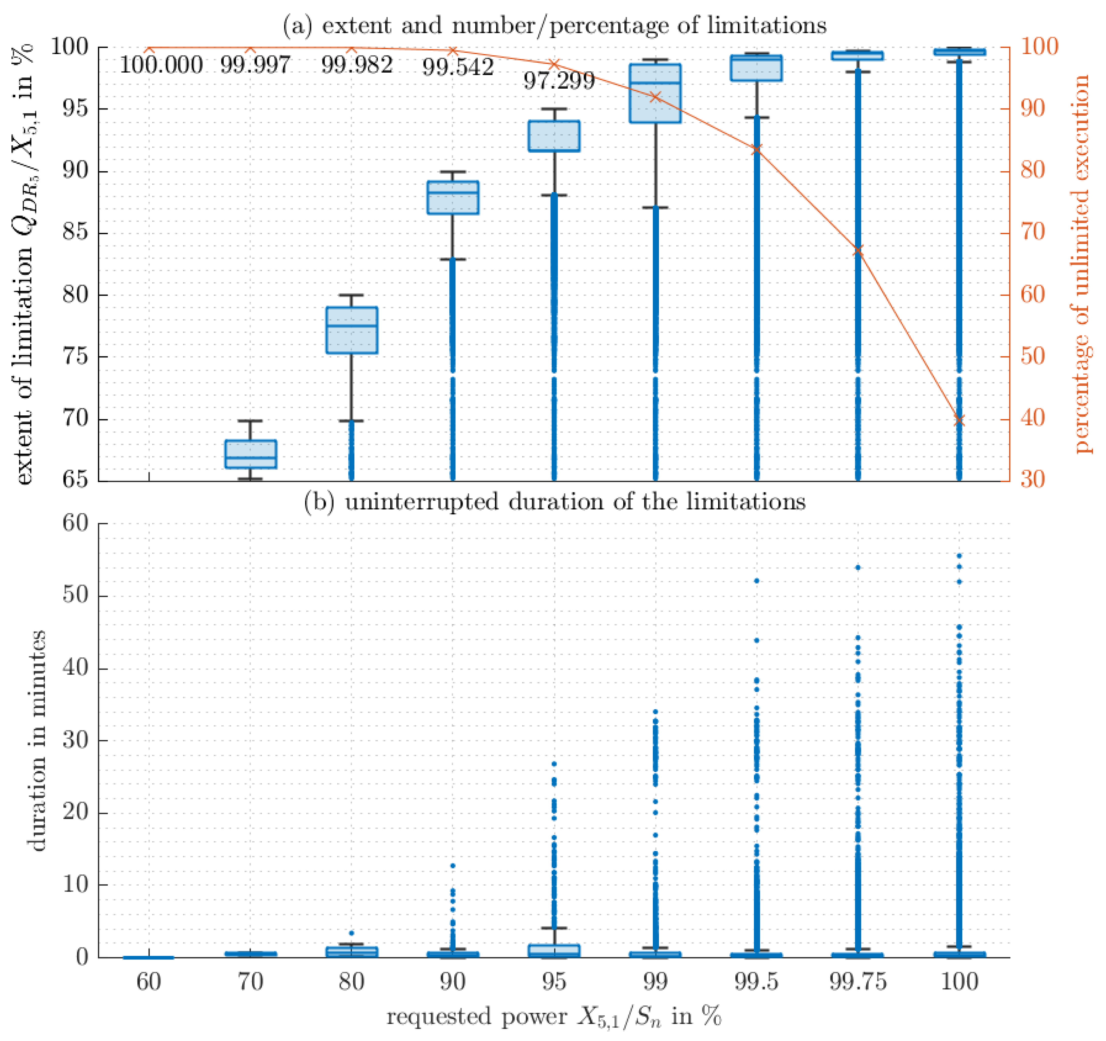
Figure 10 shows the results of this simulation depending on different but only negative values of . Figure 10a presents box plots that show the extent of the limitation on the left y-axis for each moment in which a limitation of the function occurs. Figure 10a also shows the percentage of time where limitations occur. The corresponding values can be read on the right y-axis. Figure 10b shows the uninterrupted duration of each limitation in the form of box plots. The results show function is able to provide a value of at any time. This value corresponds to a maximum limitation of function due to the function following a frequency deviation of nearly . For higher values of the percentage of limitations decreases. However, only for values of higher than the percentage of limitations is lower than 92%. As indicated by the box plots, the majority of the extent of limitations remains at values higher than 90%, even for values of . In Figure 10b the results show that the uninterrupted duration of each limitation is kept below 10 for values of up to . Regardless of the value of , the majority of durations lies below a value of 4 .
The limitation of the function Static Voltage support has two consequences. The description in Section 3.1.3 defines the use of the function as reactive power compensation, to compensate for reactive power loads. A reactive power compensation reduces the payment of tariffs for reactive energy, which business customers have to pay. A limitation therefore leads to an decrease of this payment. However, limitations of short duration can be neglected. The second consequence of a limitation is the influence on the local voltage. A limitation of the reactive power compensation leads to increasing voltage values. However, limitations of short duration do not have that much impact on power quality. The power quality regarding voltage values usually refers to mean values over a predefined duration. According to the standard EN 50160 [41], this predefined duration is ten minutes. The limitation of the function influences the local voltage values. Taking into account the requirements regarding power quality, the results in Figure 10 show that up to a value of the influence of the limitation of the function on the power quality can be neglected.
The results prove the potential of dynamic prioritization of better utilizing the power resources. Compared to a static power band assignment, where the function would not be able to utilize resources at any time, the concept of dynamic prioritization allows an utilization of power resources up to a value of without compromising the power quality. Considering an appropriate behavior during operational planning holds the potential to increase the profitability of a BESS. Based on the services summarized in Figure 1 it is an interesting future research question which other services are suitable for taking advantage of the potential of dynamic prioritization as it has been shown for the application above.
4. Conclusions
This paper investigated the real-time multi-use operation of BESS based on the concept of “dynamic prioritization”, which was presented as a novel approach inside this paper in order to handle conflicts of services. Especially during unforeseen events such as grid faults or other abnormal grid conditions, such conflicts may arise from requests for resources from several services, the overall request of which exceeds the resources of the BESS. Compared to existing approaches in literature the presented concept is not limited to specific dimensions but is based on a multi-dimensional approach, which takes into account not only active- but also reactive power components of services and their asymmetrical behavior.
Based on priorities assigned to each service it was demonstrated that the concept of dynamic prioritization is able to resolve conflicts between services. This was demonstrated based on the investigation of the behavior of a specific BESS applying the concept of dynamic prioritization during the occurrence of a short-circuit. A suitable assignment of priorities was suggested, which allows an appropriate handling of this conflict.
Besides the benefits of handling abnormal grid conditions, the investigations in this paper also proved the beneficial use of the concept of dynamic prioritization during normal grid conditions. Compared to static approaches of allocating virtual BESS for each service, the concept of dynamic prioritization holds potential for a better utilization of resources during operation at normal grid conditions. The concept of dynamic prioritization allows several services to use shared resources instead of a predefined allocation of resources. This was demonstrated based on applications such as the simultaneous provision of frequency reserves and the utilization of remaining resources of FCR by providing voltage support. Both applications showed an improved utilization of resources when using the concept of dynamic prioritization compared to static approaches. A long-time simulation of the latter application further demonstrated the potential of dynamic prioritization in order to fully exhaust the resources at any time and validated the feasibility of the concept to be considered during an operational planning phase of a multi-use operation. Assuming each of the services assigned to the functions to generate revenues, dynamic prioritization therefore may lead to higher revenues compared to static approaches.
The concept of dynamic prioritization in this paper was investigated for selected services and applications only. Future research goals therefore include the consideration of other services, the investigation of further applications and an integration of the concept of dynamic prioritization during the operational planning phase of a multi-use operation. Furthermore, future research goals comprise the consideration of key performance indicators, such as battery aging, during long-time simulation in order to be able to compare these indicators for different combinations of services.
Author Contributions
Conceptualization, J.M. and W.G.; Formal analysis, J.M.; Funding acquisition, W.G.; Methodology, J.M.; Software, J.M.; Supervision, W.G.; Visualization, J.M.; Writing—original draft, J.M.; Writing—review and editing, W.G. All authors have read and agreed to the published version of the manuscript.
Funding
This work received no external funding.
Acknowledgments
The publication of this article was supported by the Open Access Funding by TU Wien.
Conflicts of Interest
The authors declare no conflict of interest.
Nomenclature
Uppercase and lowercase letters are used to distinguish between unit-based and normalized values. Uppercase letters are used for unit-based values, while lowercase letters are used for normalized values. The unit of the normalized values is described with “pu”. To distinguish between phasors and instantaneous values, the index “t” is used for instantaneous values. Symbols in bold indicate a vector or a set. Underlined symbols in-dicate complex values. Nominal values are described with the index “n”. A summarized list of all sym-bols used in this paper can be found in Appendix B.
Appendix A. Detailed Description of Functions
Appendix A.1. F2 SoC-Management
In this paper especially for the provision of FCR the requirements regarding energy reserves to be kept available are relevant to be considered in the SoC-management. These requirements are formulated in [39] and discussed in more detail in [32]. According to Figure 2a symmetrical energy band and therefore SoC-band has to be considered for FCR.
Figure A1 shows a possible implementation of such a behavior in function .
Figure A1.
Behavior of SoC-management.

In accordance with Section 2.3 the corresponding statically- and dynamically requested powers of the function can be defined by
and
All parameters of the function are summarized in Table A1.

Table A1.
Parameters of function .
| Parameter | Parameters Description |
|---|---|
| power for SoC-management | |
| target-SoC | |
| lower limit of SoC-band | |
| upper limit of SoC-band |
According to Section 2.3 the corresponding current request of function has to be calculated based on the dynamically requested power. The current request can be calculated by
The control variables of function , therefore, can be summarized to . Although SoC-management is essential for continuous operation of the BESS, a corresponding power reservation for function may not be necessary when assuming a suitable operation management, which handles the priorities of functions, their activations and parametrization of their parameters. Therefore, the current reservation of function is defined by
Appendix A.2. F3 FR
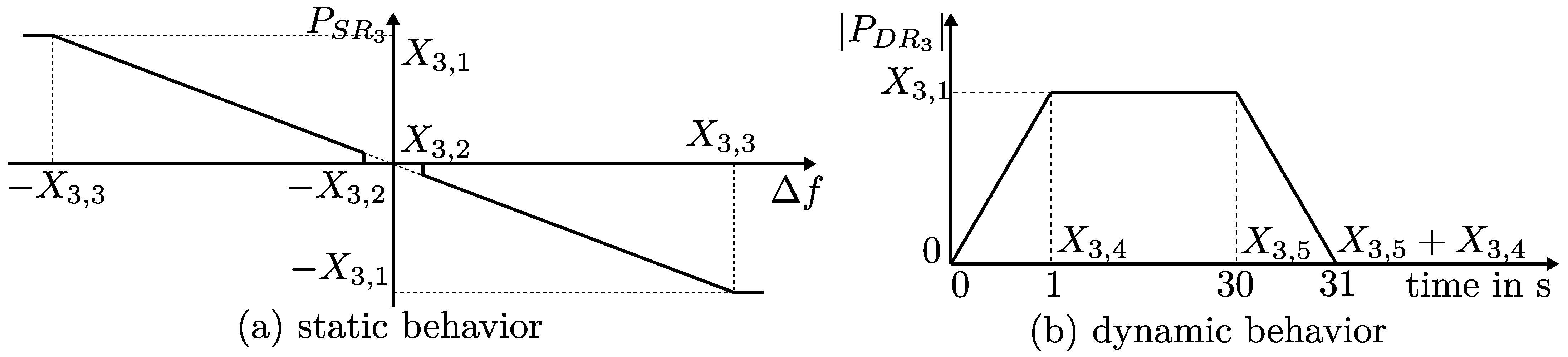
The static- and dynamic behavior of FR is illustrated in Figure A2.
Figure A2.
Static- and dynamic behavior of FR.

As shown in Figure A2a the static behavior looks identical to the static behavior of FCR, which is shown in Figure 5a. However, as already mentioned, the dynamic behavior which is shown in Figure A2b of FR looks different compared to the dynamic behavior of FCR which is shown in Figure 5b. The full activation of FR has to be reached within 1 (respectively the value parametrized in ) after a frequency deviation of 200 (respectively the value parametrized in ). However, compared to FCR, the dynamic behavior of FR includes a “release time” after which the power output returns to zero, independent from the actual frequency deviation.
In accordance with Section 2.3 the corresponding statically- and dynamically requested powers of the function can be defined by
which looks similar to and
where is related to the release time according to Figure A2. The issue with the implementation of such a release time is the dealing with part activations. For example, assuming a frequency deviation which oscillates between , the power gradient and the power output of the function change continuously. The determination of the release time for such a situation is a more complex issue than illustrated in Figure A2. It is even more difficult when the frequency deviation oscillates in a small range around the frequency deadband . The “timer” for the release time has to be defined rather clearly to deal with such part activations. The start of such a timer is defined by the moment when the frequency deviation reaches the frequency deadband and when the function is not already active ():
By defining a time mean value of the frequency deviation
the “timer” for the release time can be defined by
which is used in Equation (A6) to consider the release time. The time mean value ensures that in case of an oscillation around the frequency deadband the function becomes also inactive after a release time . Since immediately switches from 1 to 0 when the release time is reached, Equation (A6) takes into account the terms and in order to describe the gradual decrease of back to zero, as shown in Figure A2. All parameters of the function are summarized in Table A2.
Table A2.
Parameters of function .
| Parameter | Parameters Description |
|---|---|
| tendered EFR-power | |
| frequency deadband (e.g., 50 ) | |
| full activation frequency (e.g., 200 ) | |
| Full activation time ( 1 according to TERNA [19]) | |
| Release time (e.g., 30 ) |
According to Section 2.3 the corresponding current request of function has to be calculated based on the dynamically requested power. The current request can be calculated by
The control variables of function , therefore, can be summarized to . Section 3.1 describes how FCR and FR can be offered in combination by a single BESS. In such a combined operation a current reservation of function (FCR) can also be used by the function (FR), since acts much faster than and can be considered to be decoupled in time. A current reservation, therefore, is only useful when is deactivated or the tendered FR-power is higher than the tendered FCR-power. The current reservation of function , therefore, can be defined by
Appendix A.3. F4 SI
The statically requested power of SI is defined by
where the parameter represents the starting time constant and the parameter represents the apparent power of a corresponding mechanical inertia, whose behavior is imitated by the function . The parameter defines a frequency gradient deadband. The term leads to a zone-selective activation of the function, which ensures the function to request power only when it is contributory to the frequency restoration process. More details of the advantages of such a zone-selective activation are discussed in [42]. Since SI should be available instantaneously, the dynamically requested power is identical to the statically requested power:
All parameters of the function are summarized in Table A3.
Table A3.
Parameters of function .
| Parameter | Parameters Description |
|---|---|
| starting time constant of a corresponding generator whose mechanical inertia is to be imitated | |
| apparent power of a corresponding generator whose mechanical inertia is to be imitated | |
| frequency gradient deadband |
According to Section 2.3 the corresponding current request of function has to be calculated based on the dynamically requested power. The current request can be calculated by
The control variables of function , therefore, can be summarized to .
Similar to function , a certain power increment requested by function should be possible at any time in order to ensure a certain response to occurring frequency gradients. Otherwise the function would not be able to provide inertial response when other active power functions already occupy resources. In order to define a reasonable value for the current reservation, the maximum value of has to be considered. According to Equation (A12), this maximum value is depending on the maximum value of the frequency gradient and the frequency f. The maximum frequency gradient in Continental Europe today is likely to be less than 1 / [43], including situations of system split. The maximum frequency can be considered with , as the protection relays of generators usually are parametrized to disconnect at frequencies above this value. The current reservation for function can be defined by
in accordance with Equation (13).
Assuming the parameters to be , which corresponds to the starting time constant of a typical gas turbine, and , which leads to an imitation of the mechanical inertia of a gas turbine with an apparent power of , and , this would lead to a current reservation of 20%.
Appendix A.4. F5 Static Voltage Support
There are several options to define the behavior of such a static voltage support:
- according to a voltage droop control [Q(U)-control],
- according to a power factor depending on the actual active power output [-control],
- according to a fixed power factor [-control], or
- according to a parametrizeable value of reactive power (Q-control).
In this paper, the last option, Q-control, is considered and described by function . A description of the other options within the mathematical framework of Section 2.3 is easily possible. In accordance with Section 2.3 the statically requested powers of the function can be defined by
There are no special requirements on the dynamic behavior of static voltage support. Therefore, the dynamically requested power equals the statically requested power:
The current request can be calculated by
where the parameter is a parametrizable value of the reactive power. The control variables of function can therefore be summarized to . As static voltage support does not require a certain power increment but rather requires the voltage to be influenced over longer periods, there is no need for current reservation. The corresponding current reservation of function can therefore be defined by
Appendix A.5. F6 Dynamic Voltage Support
Due to these prescriptions, the direct definition of the current request of a function , which describes the dynamic voltage support, is easier than defining it via the dynamically requested power, as it was the case with foregoing functions. The Park-components of this current request of function can be defined by
where the voltage deviation in the positive-sequence system and the voltage deviation in the negative-sequence system are defined by
which represent the voltage deviations of the actual voltages in relation to the time mean value of the voltage before the occurrence of a short-circuit:
where is the root-mean-square value of . This leads to a current request of the function of
All parameters of the function are summarized in Table A4.
Table A4.
Parameters of function .
| Parameter | Parameters Description |
|---|---|
| voltage deadband (usually ) | |
| linear factor of reactive current injection in the positive-sequence system (usually this value is 2) | |
| linear factor of reactive current injection in the negative-sequence system (usually this value is 2) |
The current request of the function can be calculated based on Equation (27) with the corresponding Park-components defined above. The relation to the statically- and dynamically requested power can be calculated by
The control variables of function can therefore be summarized to .
Although the function requires a certain power increment in response to a voltage drop, Section 3.1 shows that such a power increment can be achieved by assigning this function the highest priority. Therefore, the current reservation of function is defined by
Appendix A.6. F7 Island Operation
Due to the necessary change of the control approach from a grid-following to a grid-forming control structure during island operation, the combined activation of any function in Table 1 together with function automatically becomes a member of the set , as defined in Equation (4), and must not be activated simultaneously. A grid-forming control approach has to apply a voltage control as described in [44]. This voltage control directly controls the Park-components of the voltage and based on PI-controllers.
As the voltage control of a grid-forming control approach delivers current requests which are further processed by the inverter current control, the current request of the function can be defined directly by
which is assumed to be controlled only in the positive-sequence system by the voltage control.
The relation to the statically- and dynamically requested power can be calculated by
The control variables of function can therefore be summarized to .
During island control the full current capability has to be available for function . However, as activations with other functions activated combined with are a member of the set a current reservation for the function is not necessary. Therefore, the current reservation for the function is defined by
Appendix B. List of Symbols
| normalized instantaneous current vector | |
| instantaneous value of the current in phase L1 | |
| instantaneous value of the current in phase L2 | |
| instantaneous value of the current in phase L3 | |
| current space vector in the -plane | |
| current space vector in the dq-plane | |
| reference current space vector in the dq-plane | |
| nominal current | |
| maximum current capability | |
| maximum normalized current capability | |
| reference value of the direct/active, positive-sequence component of the normalized current space vector | |
| reference value of the quadrature/reactive, positive-sequence component of the normalized current space vector | |
| reference value of the direct/active, negative-sequence component of the normalized current space vector | |
| reference value of the quadrature/reactive, negative-sequence component of the normalized current space vector | |
| direct/active, positive-sequence component of the normalized current output space vector | |
| quadrature/reactive, positive-sequence component of the normalized current output space vector | |
| phase-to-phase root-mean-square voltage vector | |
| nominal phase-to-phase voltage | |
| normalized phase-to-phase root-mean-square voltage vector | |
| normalized phase-to-neutral instantaneous voltage vector | |
| magnitude of the normalized positive-sequence voltage | |
| magnitude of the normalized negative-sequence voltage | |
| angle of the normalized positive-sequence voltage | |
| f | frequency |
| nominal frequency | |
| nominal apparent power of the BESS | |
| set of functions | |
| Function k | |
| number of functions | |
| set of activations of functions | |
| activation of function | |
| set of forbidden activation sets | |
| set of parameters of function | |
| number of parameters of function | |
| set of control variables of function | |
| number of control variables of function | |
| complex statically requested apparent power of function | |
| complex dynamically requested apparent power of function | |
| set of active power functions | |
| set of reactive power functions | |
| current request of function | |
| current reservation of function | |
| executable currents of function | |
| set of priorities | |
| priority of function | |
| set of function indices of functions with higher priorities than function has | |
| set of vectors of possible occupied currents of function | |
| maximum phase current resulting of one vector in | |
| vector in which leads to the maximum phase current | |
| set of function indices of functions their current request has to be limited | |
| function, whose current request has to be limited to values greater zero | |
| angle between positive-sequence voltage and negative-sequence voltage |
References
- IRENA. Renewable Energy Prospects for the European Union; International Renewable Energy Agency (IRENA), European Commission (EC): Abu Dhabi, UAE, 2018. [Google Scholar]
- Sterner, M.; Stadler, I. Handbook of Energy Storage: Demand, Technologies, Integration; Springer: Berlin/Heidelberg, Germany, 2019. [Google Scholar]
- IRENA. Innovation Landscape Brief: Utility-Scale Batteries; International Renewable Energy Agency (IRENA), European Commission (EC): Abu Dhabi, UAE, 2019. [Google Scholar]
- Hesse, H.C.; Schimpe, M.; Kucevic, D.; Jossen, A. Lithium-ion battery storage for the grid—A review of stationary battery storage system design tailored for applications in modern power grids. Energies 2017, 10, 2107. [Google Scholar] [CrossRef] [Green Version]
- IRENA. Electricity Storage Valuation Framework: Assessing System Value and Ensuring Project Viability; International Renewable Energy Agency (IRENA), European Commission (EC): Abu Dhabi, UAE, 2020. [Google Scholar]
- Eyer, J.; Corey, G. Energy storage for the electricity grid: Benefits and market potential assessment guide. Sandia Natl. Lab. 2010, 20, 5. [Google Scholar]
- Denis, G.; Prevost, T.; Debry, M.S.; Xavier, F.; Guillaud, X.; Menze, A. The Migrate project: The challenges of operating a transmission grid with only inverter-based generation. A grid-forming control improvement with transient current-limiting control. IET Renew. Power Gener. 2018, 12, 523–529. [Google Scholar] [CrossRef]
- Milano, F.; Dörfler, F.; Hug, G.; Hill, D.J.; Verbič, G. Foundations and challenges of low-inertia systems. In Proceedings of the 2018 IEEE Power Systems Computation Conference (PSCC), Dublin, Ireland, 11–15 June 2018; pp. 1–25. [Google Scholar]
- Crivellaro, A.; Tayyebi, A.; Gavriluta, C.; Groβ, D.; Anta, A.; Kupzog, F.; Dörfler, F. Beyond low-inertia systems: Massive integration of grid-forming power converters in transmission grids. In Proceedings of the 2020 IEEE Power & Energy Society General Meeting (PESGM), Montreal, QB, Canada, 2–6 August 2020; pp. 1–5. [Google Scholar]
- Delille, G.; Francois, B.; Malarange, G. Dynamic frequency control support by energy storage to reduce the impact of wind and solar generation on isolated power system’s inertia. IEEE Trans. Sustain. Energy 2012, 3, 931–939. [Google Scholar] [CrossRef]
- Eriksson, R.; Modig, N.; Elkington, K. Synthetic inertia versus fast frequency response: A definition. IET Renew. Power Gener. 2017, 12, 507–514. [Google Scholar] [CrossRef]
- Gundogdu, B.M.; Nejad, S.; Gladwin, D.T.; Foster, M.P.; Stone, D.A. A battery energy management strategy for UK enhanced frequency response and triad avoidance. IEEE Trans. Ind. Electron. 2018, 65, 9509–9517. [Google Scholar] [CrossRef] [Green Version]
- Campagna, G.; Landini, A.; Stefanelli, D.; Tommasi, V.; Bernabei, B.; Cantù, M.; Giovannelli, A.; Giancola, F. New flexibility services and technologies: ENEL experiences in Italy. In Proceedings of the 2020 AEIT International Annual Conference (AEIT), Catania, Italy, 23–25 September 2020; pp. 1–6. [Google Scholar]
- Rancilio, G.; Rossi, A.; Di Profio, C.; Alborghetti, M.; Galliani, A.; Merlo, M. Grid-Scale BESS for Ancillary Services Provision: SoC Restoration Strategies. Appl. Sci. 2020, 10, 4121. [Google Scholar] [CrossRef]
- Stimmer, A.; Lenz, M.; Forschauer, M.; Leonhardt, M.; Gawlik, W.; Alacs, C.; Corinaldesi, C.; Lettner, G.; Guo, Y.; Marchgraber, J.; et al. Options for the Implementation of Fast Control Reserves in the Continental European Power System. In Proceedings of the 4th Grid Service Markets Symposium; Imboden, C., Ed.; Luzern University of Applied Sciences and Arts: Lucerne, Switzerland, 2020; pp. 54–65. [Google Scholar] [CrossRef]
- Marchgraber, J.; Alács, C.; Guo, Y.; Gawlik, W.; Anta, A.; Stimmer, A.; Lenz, M.; Froschauer, M.; Leonhardt, M. Comparison of Control Strategies to Realize Synthetic Inertia in Converters. Energies 2020, 13, 3491. [Google Scholar] [CrossRef]
- National-Grid. Enhanced Frequency Response: Invitation to Tender for Pre-Qualified Parties. Website. 2018. Available online: https://www.nationalgrideso.com/sites/eso/files/documents/Enhanced%20Frequency%20Response%20ITT%20v2_2%20clean.pdf (accessed on 5 August 2020).
- ENTSO-E. Fast Frequency Reserve—Solution to the Nordic Inertia Challenge. Website. 2019. Available online: http://www.epressi.com/media/userfiles/107305/1576157646/fast-frequency-reserve-solution-to-the-nordic-inertia-challenge-1.pdf (accessed on 5 August 2020).
- TERNA. Fast Reserve. Website. 2020. Available online: https://download.terna.it/terna/Fast%20Reserve%20-%20Information%20pack_8d82fe02cbed7ad.pdf (accessed on 5 August 2020).
- International Energy Agency (IEA). Tracking Report Energy Storage. Website. 2020. Available online: https://www.iea.org/reports/energy-storage (accessed on 5 August 2020).
- Stephan, A.; Battke, B.; Beuse, M.D.; Clausdeinken, J.H.; Schmidt, T.S. Limiting the public cost of stationary battery deployment by combining applications. Nat. Energy 2016, 1, 1–9. [Google Scholar] [CrossRef]
- Olk, C.; Sauer, D.U.; Merten, M. Bidding strategy for a battery storage in the German secondary balancing power market. J. Energy Storage 2019, 21, 787–800. [Google Scholar] [CrossRef]
- Schimpe, M.; Naumann, M.; Truong, N.; Hesse, H.C.; Santhanagopalan, S.; Saxon, A.; Jossen, A. Energy efficiency evaluation of a stationary lithium-ion battery container storage system via electro-thermal modeling and detailed component analysis. Appl. Energy 2018, 210, 211–229. [Google Scholar] [CrossRef]
- Englberger, S.; Hesse, H.; Hanselmann, N.; Jossen, A. SimSES Multi-Use: A simulation tool for multiple storage system applications. In Proceedings of the 2019 16th International Conference on the European Energy Market (EEM), Ljubljana, Slovenia, 18–20 September 2019; pp. 1–5. [Google Scholar]
- Namor, E.; Sossan, F.; Cherkaoui, R.; Paolone, M. Control of battery storage systems for the simultaneous provision of multiple services. IEEE Trans. Smart Grid 2018, 10, 2799–2808. [Google Scholar] [CrossRef] [Green Version]
- Brogan, P.V.; Best, R.; Morrow, J.; Duncan, R.; Kubik, M. Stacking battery energy storage revenues with enhanced service provision. IET Smart Grid 2019, 3, 520–529. [Google Scholar] [CrossRef]
- Almasalma, H.; Deconinck, G. Simultaneous Provision of Voltage and Frequency Control by PV-Battery Systems. IEEE Access 2020, 8, 152820–152836. [Google Scholar] [CrossRef]
- Kucevic, D.; Tepe, B.; Englberger, S.; Parlikar, A.; Mühlbauer, M.; Bohlen, O.; Jossen, A.; Hesse, H. Standard battery energy storage system profiles: Analysis of various applications for stationary energy storage systems using a holistic simulation framework. J. Energy Storage 2020, 28, 101077. [Google Scholar] [CrossRef]
- Truong, C.N.; Schimpe, M.; Bürger, U.; Hesse, H.C.; Jossen, A. Multi-use of stationary battery storage systems with blockchain based markets. Energy Procedia 2018, 155, 3–16. [Google Scholar] [CrossRef]
- Electric Power Research Institute (EPRI), Storage Value Estimation Tool (StorageVET). 2020. Available online: https://www.storagevet.com/ (accessed on 5 August 2020).
- Arteaga, J.; Zareipour, H. A price-maker/price-taker model for the operation of battery storage systems in electricity markets. IEEE Trans. Smart Grid 2019, 10, 6912–6920. [Google Scholar] [CrossRef]
- Marchgraber, J.; Gawlik, W.; Wailzer, G. Reducing SoC-Management and losses of battery energy storage systems during provision of frequency containment reserve. J. Energy Storage 2020, 27, 101107. [Google Scholar] [CrossRef]
- Marchgraber, J.; Gawlik, W. Dynamic Voltage Support of Converters during Grid Faults in Accordance with National Grid Code Requirements. Energies 2020, 13, 2484. [Google Scholar] [CrossRef]
- European Union. Commission Regulation (EU) 2017/1485; Establishing a Guideline on Electricity Transmission System Operation; System Operator guideline (SO GL). Website. 2017. Available online: https://eur-lex.europa.eu/legal-content/EN/TXT/?uri=CELEX%3A32017R1485 (accessed on 5 August 2020).
- E-Control. Technische und Organisatorische Regeln für Betreiber Und Benutzer von Netzen: TOR Erzeuger: Anschluss und Parallelbetrieb von Stromerzeugungsanlagen des Typs B. 2019. Available online: https://www.e-control.at/documents/1785851/1811582/TOR+Erzeuger+Typ+B+V1.0.pdf/a9a7e5ae-5842-caa9-d2c0-93be4b6e0802?t=1562757801048 (accessed on 27 June 2019).
- VDE. Technische Regeln für den Anschluss von Kundenanlagen an das Mittelspannungsnetz und deren Betrieb (TAR Mittelspannung. 2017. Available online: https://www.vde.com/de/fnn/arbeitsgebiete/tar/tar-mittelspannung-vde-ar-n-4110 (accessed on 27 June 2019).
- Wurm, M. 110-und 30-kV-Netzkurzschlussversuche mit einem 2, 2-MWh-Batteriespeicher. e & i Elektrotechnik und Informationstechnik 2019, 136, 21–30. [Google Scholar]
- UCTE. Load-Frequency Control and Performance; Appendix A1. Website. 2004. Available online: https://www.entsoe.eu/fileadmin/user_upload/_library/publications/entsoe/Operation_Handbook/Policy_1_Appendix%20_final.pdf (accessed on 19 March 2019).
- ENTSO-E. All CE TSOs’ Proposal for Additional Properties of FCR in Accordance with Article 154(2) of the Commission Regulation (EU) 2017/1485 of 2 August 2017 Establishing a Guideline on Electricity Transmission System Operations. 2018. Available online: https://consultations.entsoe.eu/system-operations/synchronous-area-operational-agreement-policy-1-lo/supporting_documents/Article%20A2_Additional%20properties%20of%20FCR%20002.pdf (accessed on 27 June 2019).
- ENTSO-E. Continental Europe; Significant Frequency Deviations—January 2019. 2019. Available online: https://eepublicdownloads.entsoe.eu/clean-documents/news/2019/190522_SOC_TOP_11.6_Task%20Force%20Significant%20Frequency%20Deviations_External%20Report.pdf (accessed on 27 June 2019).
- OVE. OVE EN 50160:2011. Voltage Characteristics of Electricity Supplied by Public Electricity Networks 2016. p. 36. Available online: https://shop.austrian-standards.at/action/de/public/details/383226/OEVE_OENORM_EN_50160_2011_03_01 (accessed on 23 June 2020).
- Gawlik, W.; Alacs, C.; Marchgraber, J.; Guo, Y.; Anta, A.; Kathan, J.; Weiss, B.; Oberhauser, K.; Lenz, M.; Froschauer, M.; et al. Improving synthetic inertia provision by Power Electronic Interfaced Power Sources to support future system stability. e & i Elektrotechnik und Informationstechnik 2020, 137, 460–469. [Google Scholar] [CrossRef]
- ENTSO-E RG-CE System Protection and Dynamics Sub Group. Frequency Stability Evaluation Criteria for the Synchronous Zone of Continental Europe. 2016. Available online: https://eepublicdownloads.entsoe.eu/clean-documents/SOC%20documents/RGCE_SPD_frequency_stability_criteria_v10.pdf (accessed on 27 June 2019).
- Marchgraber, J.; Gawlik, W. Investigation of Black-Starting and Islanding Capabilities of a Battery Energy Storage System Supplying a Microgrid Consisting of Wind Turbines, Impedance- and Motor-Loads. Energies 2020, 13, 5170. [Google Scholar] [CrossRef]
Figure 1.
Categorization of services for which Battery Energy Storage Systems (BESS) are suited.

Figure 2.
Concept of allocation of virtual BESS for each function on the example of assignment of energy bands for each function in a specific time slot. The grey color marks the reserved energy band of corresponding functions.
Figure 2.
Concept of allocation of virtual BESS for each function on the example of assignment of energy bands for each function in a specific time slot. The grey color marks the reserved energy band of corresponding functions.

Figure 3.
Concept of allocation of virtual BESS for each function on the example of static assignment of power bands for each function in a specific time slot. The grey color marks the currently occupied share of the power band of the corresponding function.
Figure 3.
Concept of allocation of virtual BESS for each function on the example of static assignment of power bands for each function in a specific time slot. The grey color marks the currently occupied share of the power band of the corresponding function.

Figure 4.
Concept of dynamic prioritization of functions.

Figure 5.
Static- and dynamic behavior of FCR.

Figure 6.
Dynamic prioritization during short-circuit event.

Figure 7.
Vector diagrams of the space vectors in the -plane before (a) and during (b) the short-circuit event. In (a) and (b) the vectors L1, L2 and L3 all have a length of . (b) shows that during the short-circuit event the projection of on L3 equals the maximum current capability .
Figure 7.
Vector diagrams of the space vectors in the -plane before (a) and during (b) the short-circuit event. In (a) and (b) the vectors L1, L2 and L3 all have a length of . (b) shows that during the short-circuit event the projection of on L3 equals the maximum current capability .

Figure 8.
Dynamic prioritization during reference incident.

Figure 9.
Dynamic prioritization during active functions , FCR, , state of charge (SoC)-Management, , Static Voltage Support.
Figure 9.
Dynamic prioritization during active functions , FCR, , state of charge (SoC)-Management, , Static Voltage Support.

Figure 10.
Simulation results of the limitation of the function static voltage support during long-time simulation in Matlab/Simulink.
Figure 10.
Simulation results of the limitation of the function static voltage support during long-time simulation in Matlab/Simulink.

Table 1.
Overview of selected functions.
| Function | Function Description |
|---|---|
| FCR | |
| Management of the state of charge (SoC-management) | |
| FR | |
| SI | |
| Static voltage support | |
| Dynamic voltage support | |
| Island operation |
Table 2.
Parameters of function .
| Parameter | Parameters Description |
|---|---|
| tendered FCR-power | |
| frequency deadband (usually 10 ) | |
| full activation frequency ( 200 according to SOGL [34]) | |
| Full activation time ( 30 according to SOGL [34]) |
Table 3.
Unpredictability of selected functions.
| Function | Unpredictability | Function Description |
|---|---|---|
| (a) | FCR | |
| (a) | Management of the state of charge (SoC-management) | |
| (a) | FR | |
| (b) | SI | |
| - | Static voltage support | |
| (b) | Dynamic voltage support | |
| (b) | Island operation |
Publisher’s Note: MDPI stays neutral with regard to jurisdictional claims in published maps and institutional affiliations. |
© 2021 by the authors. Licensee MDPI, Basel, Switzerland. This article is an open access article distributed under the terms and conditions of the Creative Commons Attribution (CC BY) license (http://creativecommons.org/licenses/by/4.0/).
Share and Cite
MDPI and ACS Style
Marchgraber, J.; Gawlik, W. Dynamic Prioritization of Functions during Real-Time Multi-Use Operation of Battery Energy Storage Systems. Energies 2021, 14, 655. https://doi.org/10.3390/en14030655
AMA Style
Marchgraber J, Gawlik W. Dynamic Prioritization of Functions during Real-Time Multi-Use Operation of Battery Energy Storage Systems. Energies. 2021; 14(3):655. https://doi.org/10.3390/en14030655
Chicago/Turabian StyleMarchgraber, Jürgen, and Wolfgang Gawlik. 2021. "Dynamic Prioritization of Functions during Real-Time Multi-Use Operation of Battery Energy Storage Systems" Energies 14, no. 3: 655. https://doi.org/10.3390/en14030655
Note that from the first issue of 2016, this journal uses article numbers instead of page numbers. See further details here.