Case Study of Residential PV Power and Battery Storage with the Danish Flexible Pricing Scheme


Department of Energy Technology, Aalborg University, 9220 Aalborg, Denmark
*
Author to whom correspondence should be addressed.
Energies 2019, 12(5), 799; https://doi.org/10.3390/en12050799
Submission received: 8 January 2019
/
Revised: 15 February 2019
/
Accepted: 20 February 2019
/
Published: 28 February 2019
Abstract
:The economic viability of renewable energy generation is vital for sustainability. Ensuring that optimal operation is always achieved, using energy management systems and control algorithms, is essential in this endeavor. Here, a new real-time pricing scheme, the Danish flexible pricing scheme, illustrates how residential PV and battery systems can optimize the electricity bill of households, without changing consumption behavior or providing grid services in exchange. This means that the only addition is PV production, storage, and control. A case study is constructed from Danish household consumption data, irradiance measurements, and recorded spot prices. With the input data, the pricing scheme, and the energy flow, simulation models are computed in MATLAB, thereby validating the algorithmic potential and finding the best strategy for charging and discharging the energy storage unit. Different methods are compared to list the viable options and evaluate them, based on the economic feasibility for the household. Furthermore, a discussion of the system implementation is also included to highlight technical difficulties, co-integration opportunities, short-comings, and advantages present in the case study. In conclusion, it is possible to make renewable energy generation, and storage, viable for a Danish residential household under the new pricing scheme.
1. Introduction
Concerns about the implications of energy production, transmission, and consumption with respect to the environmental challenges that the world is currently faced with have sparked tremendous research into sustainable alternatives and the consequences if changes are not made with sufficient determination [1,2,3]. A shift in the energy mix, from fossil fuels to renewable energy sources (RES), has been made a priority, and the aftermath presents several challenges to the energy industry. Many of the RES are inherently distributed energy resources (DES), which means that the production of energy is moved from centralized to decentralized power plants, of varying sizes and controllability. Therefore, problems naturally arise when the electrical grid is forced to change [4]. Some of the challenges that this presents are natural [5,6], as new initiatives arise and technological advancements are weaved into the mix [7]. Others are inherent to the nature of intermittent sources [8] or related to the power electronic interfaces of wind power systems (WPS), photovoltaic power (PV) plants, among others [9]. A crucial variable is the levelized cost of energy [10], as the economic motivation is prominent.
From the consumers’ perspective, the electricity market is mostly a supply of energy, traded for monetary value. This has been coupled with real-time pricing (RTP), to prioritize RES [11,12,13]. In turn, technical advancements in consumer technology and systems have been made to utilize RTP schemes, including behind-the-meter storage (BTMS) systems, where energy storage is installed locally to minimize the electricity bill of the consumers [14,15,16,17,18]. As the RTP schemes become more widespread, so will BTMS. A country that is in the process of installing smart-meters and introducing an RTP scheme is Denmark.
2. The Flexible Pricing Scheme
In Denmark, the electricity market has many operators influencing the energy mix and pricing for consumers, which also complicates the market pricing procedure. A brief overview is presented to introduce this, with emphasis on the most influential actors.
The Danish transmission system operator (TSO) is Energinet. Its role is to run the transmission grid, ensure energy balance in the grid, and create the framework for a well-functioning electricity market. Datahub is responsible for data integrity and validity, reporting to the European electricity exchange, Nord Pool, owned by the European TSOs. Operators responsible for balancing trade energy on the exchange, which is supplied by plant owners, bought by suppliers, and re-sold to consumers. The energy is transported through the transmission grid and then through a distribution grid, owned by various grid companies, to the consumer. Despite this market structure, with hourly-quoted RTPs, the Danish residential consumers pay a fixed price for electricity (DKK/kWh) along with various tariffs, taxes, subscriptions, and profits to the involved operators in the electrical energy market.
In December 2017, the Danish Energy Agency and Energinet began imposing a new price structure, called the flexible pricing scheme (FPS) (DA: Flexafregning). Within this, the fixed price for electricity will be substituted by the hourly-quoted (flexible) spot price from Nord Pool, an RTP scheme. Consumers are thereby incentivized to adopt more environmentally-friendly consumer habits by favouring an energy mix of inexpensive RES instead of fossil fuels [19]. Additionally, modifications in consumer behaviour, seen from the grid, can be dynamically incentivized through price changes.
The FPS was first introduced in December 2017 by two Danish grid companies, Radius (in the Copenhagen area) and NRGI Net (in the Eastern Jutland area). A requirement for the FPS is remote electricity meters, installed in the households. The FPS is planned to be fully implemented on a national scale by 2020.
A new pricing scheme has the potential to influence consumer behaviour, but will also inherently alter which energy investment options are economically viable and to what degree.
While there are options for consumers to change behaviour dependent on external factors and scheduling schemes [20,21], there will still be a segment of them who cannot or does not wish to change their consumption behaviour. RES and BTMS with intelligent control, linked to Nord Pool spot prices, could be a viable option, with the FPS. This involves implementing an energy management algorithm, which considers the behaviour of the residential household load, as seen from the grid— producing/selling energy when prices are high, and consuming/buying energy when prices are low. The general idea has been investigated in the literature, in relation to other countries and cases [22,23,24,25,26,27]. This paper investigates BTMS with unchanged energy consumption behaviour in Denmark for residential consumers. It furthermore addresses the technological challenges associated with it and discusses the economic validity of the solution.
The current pricing scheme and FPS are summarized in Table 1 and Table 2, respectively. Please note that E = consumption −production. From the tables, these two schemes primarily differ in two ways: (1) prices for electricity are either fixed or tied to the hourly-quoted spot price, and (2) the surplus subsidiary is lowered from 600 to 250 DKK/MWh. These changes are significant because the residential energy balance under the FPS now relates to the instantaneous balance of energy, and not only to the annual accumulated values, net-transfer. This motivates a monitoring and control system for households to minimize the electricity bill. It is difficult to provide a simplified example for calculating the difference in the electricity bill for a household with PV under the new and old pricing schemes. This is due to a large dependence on the correlation between price-production, price-consumption, and the instantaneous overlap between production and consumption. These factors influence the results so highly that a simplification cannot be representative, i.e., simulations should be made in each case to calculate the difference.
3. Danish Case Study
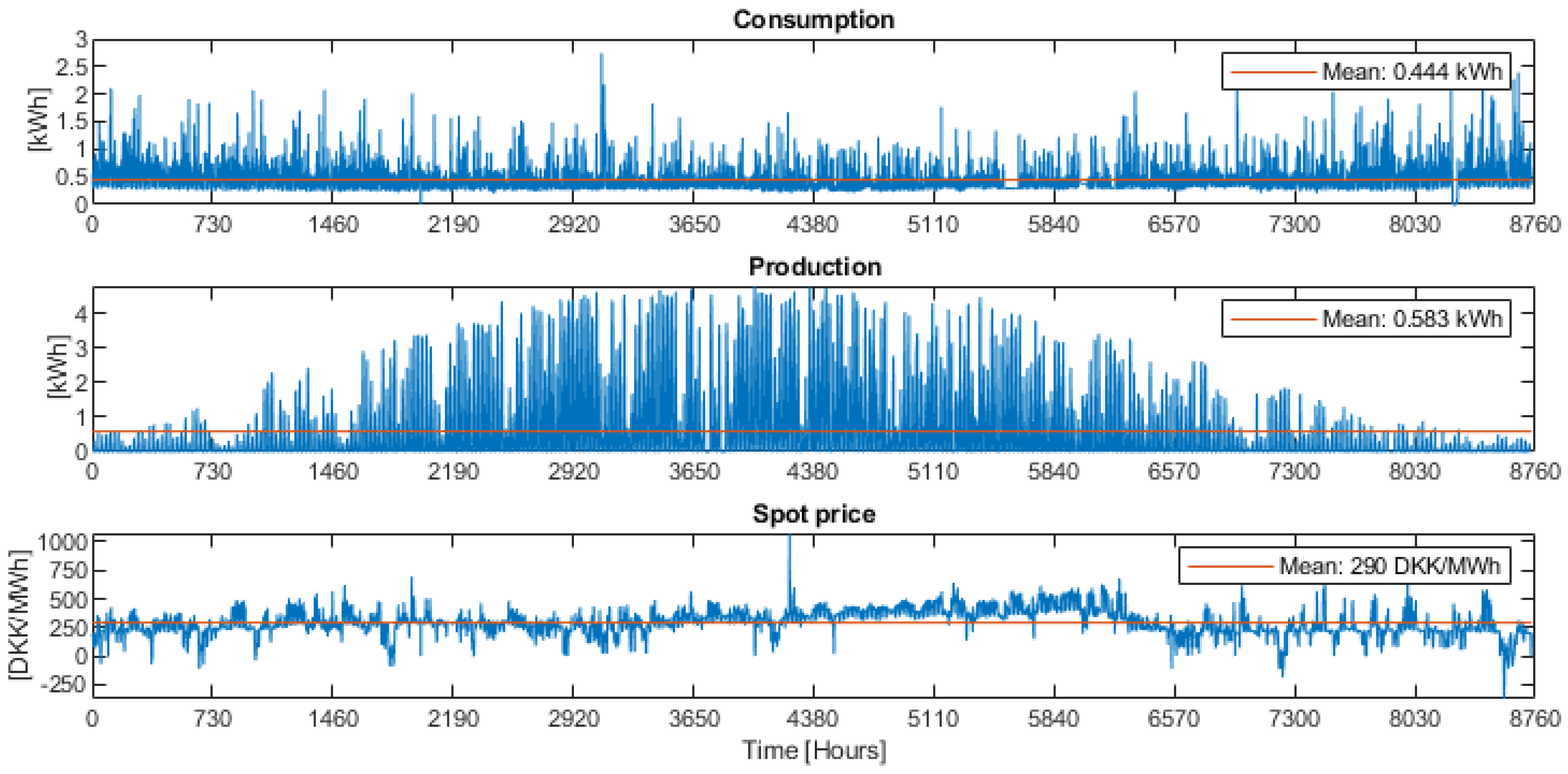
A case study of a randomly-selected Danish household in the Thisted area was used to assess the economic validity. The household did not have electric heating or any renewable energy production, so the energy consumption time series data were purely from home appliances (lighting, cooking, refrigeration, cleaning, etc.). A plot of the time series is shown in Figure 1. On a yearly basis, the household had a consumption of 3.900 kWh. To simulate the PV system, a time series of measured irradiance has been converted to energy production from the data sheet values of a 6-kWp system. PV power (including inverter) is, simply, related to irradiance, r, panel area, A, and system efficiency, , through,
which states that power can be calculated by the incident irradiance per area times the actual area, including a measure of efficiency for conversion. From the PV panel data sheet values and inverter efficiency of 90% (low estimate for worst case), the system efficiency is calculated from (1) as:
As the panel efficiency has been determined, energy production within a given hour () can be calculated by integrating irradiance, yielding the maximum possible energy output, and then multiplying by the system efficiency to obtain the output,
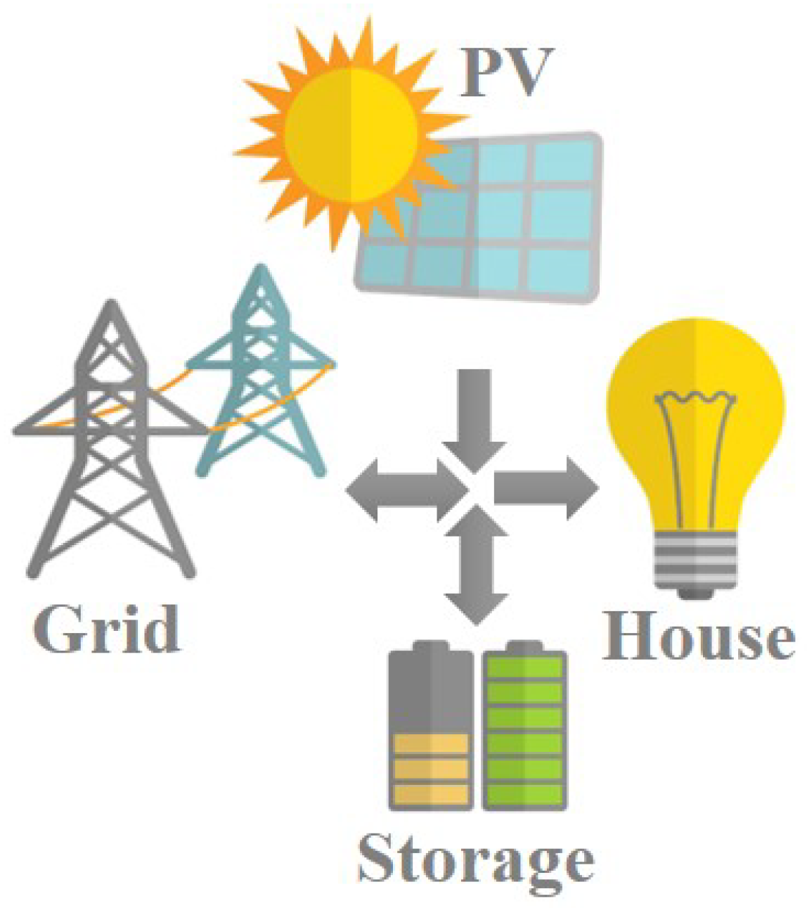
The PV energy production time series is shown in Figure 1. This amounts to 5.100 kWh per year, making the household a net-producer seen from the grid. Energy storage is added to the system in the form of a 13.5-kWh, AC-coupled stand-alone Li-ion battery system (storage and inverter), with a power rating of 5 kWp and a round-trip efficiency of 90% (5% for charging and discharging, respectively). The residential energy system is schematically depicted in Figure 2.
Prices of energy are recorded by Datahub and are available online for the Danish grid, DK1, synchronized with western Europe. This time series is also shown in Figure 1. The PV, storage, and combined PV with storage systems pose an investment for the consumer, which must be accounted for when solutions are compared. Therefore, investment, annual service, and annuity are incorporated into the analysis, for each of the three cases, shown in Table 3. The annual interest was assumed to be 3.95%, based on Danish credit institutions.
Simulations were done with a MATLAB script that loops through each hour of the past year and records the system behavior, consumption, production, and spot price to calculate the yearly electricity bill as a metric for performance. This is done for a select set of configurations,
- Only consumption (current pricing scheme);
- Only consumption (FPS);
- Consumption with FPS and PV;
- Consumption with FPS, PV, and storage (simple);
- Consumption with FPS, PV, and storage (optimal).
These were all compared based on their relative economic viability (investment and reduction in electricity bill). As shown above, this was done in relation to two energy management algorithms for battery storage: simple and decision tree-based (referred to as “optimal”, due to the decision process).
4. Energy Management Algorithms
For comparison, two algorithms are covered in the following subsections.
4.1. Simple Strategy
The first is simply to charge the battery with PV power when there is excess production (as opposed to selling it to the grid) and discharging the battery when PV production cannot cover consumption (instead of drawing from the grid). When the battery is depleted, energy is supplied from the grid, without regards to the prices. When PV power is available, but the battery is fully charged and the load is met, energy is sold to the grid.
4.2. Optimal Decisions
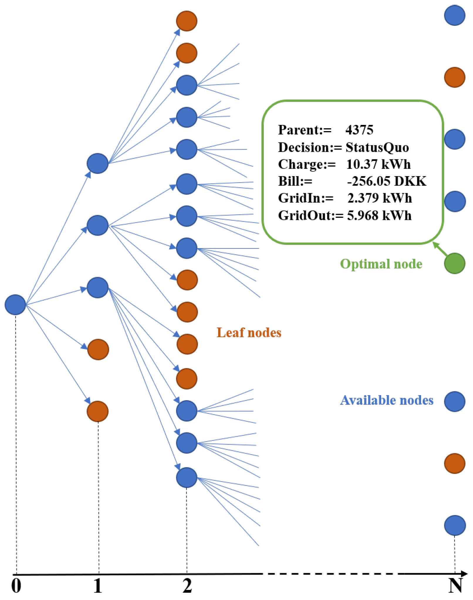
The second attempts to calculate an optimal decision flow for the battery charge, with respect to the electricity bill, within a prediction horizon (N). This is done by assuming that the controller has a finite number of choices each hour (to simplify the control objective), corresponding to the hourly price changes, in this case five. These are: (1) do not use the battery (always applicable); (2) discharge the battery to the grid (battery charge > 0 kWh); (3) discharge battery to the household (battery charge > 0 kWh); (4) charge battery from the grid (battery charge < 13.5 kWh); (5) charge battery from PV (battery charge < 13.5 kWh). Realistically, not all of these options are available in every time-step since the battery can be fully charged or discharged, and PV energy may not be available. However, the optimal algorithm works by constructing the full decision tree with all available options every hour of the prediction horizon and then selecting the outcome with the lowest electricity bill, providing the controller with a decision for every hour. If all options are available for all time-steps (no leaf/terminal nodes in the decision tree), the number of nodes is where N is the prediction horizon, i.e., number of hours.
For a case of five options and a prediction horizon of 12 h, the number of nodes becomes approximately 300 million, which is not computationally feasible. Therefore, prediction horizons of less than 12 h will be used in this paper.
An example of a decision tree is shown in Figure 3. Each node contains information about the parent (decision in the previous time-step), the current decision (status quo, discharge-grid, discharge-house, charge-Grid, charge-PV), battery state-of-charge (SoC), electricity bill, and accumulated energy transferred to and from the grid. This allows the nodes at the final time-step to be inspected for an optimal solution and then back-tracing the decisions that yield that particular outcome.
The procedure is repeated every hour, to ensure that the controller is always using the most recent data and using the optimal decision to match the real-time price progression. Additionally, the algorithm needs a second part, to feed in the necessary data every hour, namely N-hour forecasts of prices, PV production, and consumption, which are beyond the scope of this paper. As they will introduce uncertainty and thereby reduce the accuracy of the optimal solution, a short discussion of this is presented in the following section.
5. Forecasting of Time Series
As previously mentioned, this paper does not address the issues of uncertainty imposed by forecasting prices, residential load, and PV production. As these will inevitably influence the viability of the solution, they are briefly mentioned in this section, with references to other work in the literature.
There are many different approaches to forecasting these variables, such as support vector machines (SVM) with kernel functions or soft margins, various deep learning neural networks (NN), and seasonal auto-regression integral moving average exogenous (SARIMAX) time series models, to name a few. In this particular case, the seasonal trend is more important than the absolute value, i.e., a large error can be tolerated, as long as the volatility and seasonality are accurately represented in the forecasting model. Therefore, it is difficult to draw conclusions, based on previous work where only the average error over the entire prediction horizon was reported. Mohsenian-Rad and Leon-Garcia reported a 17% average forecasting error for a 24-h prediction horizon using a weighted average price predictor. They simulated that this results in a 1.5% increase in cost for the consumer [12]. However, the results are difficult to generalize.
Other work with forecasting, such as Khan and Jayaweeara, reported a mean absolute percentage error (MAPE) of around 10% for yearly aggregated consumer forecasts, with k-means machine learning for classification of customer segments and a neural network for forecast regression [21]. Anbazhagan and Kumarappan [30] studied electricity price forecasting errors, which generally range from approximately 5% to 36%. In comparison, [31] reported short-term electric load forecasting with between 1% and 3% error.
As the forecasting error is dependent on methodology, pricing scheme, modeling, computational effort, and data availability, it is difficult to make an assessment of the impact on the economic viability for the consumer in this particular case study. A deviation of 1 to 2% can be tolerated, but this will also depend on the prediction horizon. Therefore, it is suggested that predictions be incorporated into a future analysis, if possible.
6. Simulation and Results
Running the simulations yielded profiles for battery charge, production, and consumption throughout the year. However, the most important metric was the final electrical bill. This number represents the system performance, along with investment cost. Table 4 summarizes the results.
A notable difference can be seen between the current pricing scheme and the new FPS. This is due to three things: (1) the fixed price used, (2) RTP level, and (3) price-consumption correlation. In this case, the consumer was predicted to have a reduction of the electricity bill of 1.041 DKK, without taking any action. The addition of 6 kWp PV significantly reduced the electrical bill even further (830 DKK), but not enough to off-set the investment as the total yearly cost (11.497 DKK) was higher than without PV (8.151 DKK). With the FPS, PV, and a 10-h prediction horizon, the addition of storage substantially reduced the electricity bill, towards a monetary gain. Again, this is not enough to counteract the investment with the simple energy management algorithm. With the optimal algorithm, a clear trend can be seen when the prediction horizon is increased from h to h. Breaking even was achieved when , and the electricity bill was further decreased as the horizon was increased. Simulations for took approximately five days for a computer with 32 GB RAM and six 3.60-GHz CPU cores. Therefore, results for have not been obtained.
The best option, listed here, was FPS incl.PV and storage with a 10-h prediction horizon. From Table 4, the difference between this and FPS without an energy management system was DKK/year, with loan service over the first 10 years. After the initial 10 years, the loan is paid back, and the earnings would be DKK/year, not including repairs, maintenance, and replacement. For a 20-year period (10 years with loan service and 10 years without), the total difference between FPS and FPS with a PV and storage system would be DKK. This is significant for its viability, as it poses an opportunity for the consumers to not only break even, but also to have a reasonable return on their investment.
7. Limitations and Further Work
From the previous section, it is evident that the methods presented here pose an opportunity for PV and storage in the residential sector, under the new Danish FPS. As the prediction horizon was increased, the algorithm approached a yearly optimum, for the energy management scheme, and minimized the household electricity bill. However, the results presented here are based on assumptions and are subject to constraints that limit the potential to extrapolate and scale indefinitely. These assumptions and limitations are discussed below.
Firstly, the time series forecasting has been omitted for simplicity. However, this part has the potential to influence the viability significantly. Perfect forecasting is impossible to achieve in practice, and even though the progression of the time series is more important than the exact values, this should be addressed.
The second is data availability. Residential consumers may not have historical data records of energy consumption and/or PV production. The algorithm must therefore run, without data, while the necessary inputs are gathered. As data become available, the performance can be improved with higher fidelity forecasting estimates. Price data are available on Datahub, and the system therefore, only, needs an Internet connection to access the vast records of historical price developments.
Another issue is the integration with other controllers in the system. Since this algorithm provides the overall guideline for what action is preferred within the hour, another controller must be designed to actuate this. If the choice is to charge the battery from PV, the intra-hour controller must standby, prepared to route power from the PV system, whenever power comes on-line, and reroute power when the battery is fully charged. Additionally, this paper has assumed no overlap between PV production and household consumption. Even though the pricing scheme refers to instantaneous energy balance and power transfer, this is not a realistic case. The intra-hour controller must also account for this, possibly by using the battery as a buffer, to achieve the overall command objective.
The optimal energy management problem described here is continuous in nature, but is discretized into five available options, per hour. This is done to simplify the solution process; however, other choices may lead to better solutions with higher pay-offs.
Computational requirements by the system processor and memory are currently quite high, as a real-time system must finish the optimization routine within the hour to avoid process overrun. Since there is an obvious trade-off between economic viability/profit, prediction horizon, and computational effort, a reduction in algorithmic complexity and processor/memory requirements will enable the system to generate better solutions and possibly increase profits beyond the current prediction. With respect to this, it would be desirable to have an operable heuristic alternative to the brute-force approach described herein, since this is where the bulk of the effort is spent, i.e., the bottleneck.
Another assumption lies in the representative nature of the available data. The correlation between price and consumption time series is imperative. A high positive correlation merits the investment into storage and PV, as the average price of energy is relatively high. Conversely, a high negative correlation leads to a relatively low average price of energy, meaning that this solution has less merit. It is still possible to produce from PV, store it, and sell the energy when prices are high, yet it cannot be coupled with a lower price for consumption, which neutralizes half of the control advantage. The consumption and price time series used in this case study have a cross-correlation coefficient of 0.775, with a p-value of 0.8 (with the null-hypothesis that there is no correlation, i.e., the correlation is statistically significant). The result of this is that the household is a good case for the application of this energy management system.
Additionally, an important assumption behind the motivation for this work is that the consumers intend to maintain their consumption habits, regardless of the electricity price developments. This assumption in itself may be valid to some extent; nevertheless, initiatives such as smart-grid, smart-appliances, and electric vehicle (EV) charge controllers open up the possibility of additional flexibility for the residential energy management system, as consumption can be, partially, used to decrease costs even further. Consequently, this adds another layer of complexity, though the overall methodology described in this paper could still be valid or used to form the basis for further work.
Lastly, for a given household, with a fixed pricing scheme, there is an optimal size for PV and storage systems. Analogously, it would be desirable to develop an approach to determine the optimal storage capacity and PV system with the FPS. Factors such as price-consumption correlation, base load, and consumption variance could influence how the system is scaled and can maximize investment return. Additionally, other options for renewable energy production and storage technologies could also be included in the analysis as these also have the potential to influence the economic viability. It is also possible that some cases cannot support production, as it does not off-set the investment, and storage is the only addition that makes economic sense. Therefore, a full analysis of all possible scenarios will reveal what solution is best in the given case. For a complete analysis and evaluation of the economic impact, from the installation of PV and storage, it is also prudent to briefly mention the household market price [32]. In the Danish market, this is positively correlated with the Energy Certificate rating [33], which is improved by renovations with renewable energy installation. Therefore, a monetary gain, besides reduction in the electrical bill, is also added in the form of an increase in property value. The exact value of this is complicated to assess and goes beyond the scope of this paper, but it is worth mentioning that it also has an impact on the economic viability.
8. Conclusions
Changes in the energy sector are occurring in more ways than one. The electrical energy mix is shifting from fossil fuels to renewable; decentralized generation is being favored over centralized generation; and different economic initiatives such as RTP enable BTMS solutions. This is also seen in Denmark with the new FPS being implemented over the next few years. To capitalize on this and support the integration of renewable energy sources in the residential sector, a case study has been formulated and analyzed, including energy management. The choice of algorithm has potential to influence the viability of PV and storage, without altering consumer behavior or installing any other smart technology in the household. This is done by predicting PV production, residential consumption, and energy spot prices a certain number of hours in advance and then calculating the best course of action for the storage unit to charge, discharge, supply the load, sell energy to the grid, or buy when prices are low. As the prediction horizon increases, the algorithm minimizes the electricity bill, thereby increasing the profits. It remains inconclusive whether this off-sets the uncertainty of the predictions or where the optimal prediction horizon lies, as further work is needed to verify the results conclusively and implement the algorithm. By focusing not on renewable energy or CO emissions, but rather relying on the market economics, this methodology is shown to make storage and RES viable for Danish households in the foreseeable future.
Author Contributions
Conceptualization, J.B.N., T.K., and D.S.; methodology, J.B.N., T.K., and D.S.; software, J.B.N.; validation, J.B.N.; formal analysis, J.B.N.; investigation, J.B.N.; resources, T.K. and D.S.; data curation, T.K.; writing, original draft preparation, J.B.N.; writing, review and editing, J.B.N., T.K., and D.S.; visualization, J.B.N.; supervision, T.K. and D.S.
Funding
The authors acknowledge the support of the Danish Energy Technology Development and Demonstration Program (EUDP) through the project PVST – PV+STorage Operation and Economics in distribution systems, project nr. 12,551.
Acknowledgments
The authors would like to express their gratitude towards the people who have contributed with assistance, knowledge, and data curation for this work. Alan Sørensen from Spar Nord has aided in establishing the economic analysis for financing the various systems. Rolf Kirk from Thy-Mors Energi provided data of residential consumption for the case study. Preben Høj Larsen from Energinet was instrumental in understanding the new pricing scheme, FPS.
Conflicts of Interest
The authors declare no conflict of interest. The funders had no role in the design of the study; in the collection, analyses, or interpretation of data; in the writing of the manuscript; nor in the decision to publish the results.
References
- Hansen, J.; Sato, M.; Ruedy, R. Perception of climate change. Proc. Nat. Acad. Sci. USA 2012, 109, 14726–14727. [Google Scholar] [CrossRef] [PubMed]
- U.S. EPA. Climate Impacts on Energy. 2017. Available online: https://19january2017snapshot.epa.gov/climate-impacts/climate-impacts-energy_.html (accessed on 19 January 2017).
- U.S. Department of Energy. Climate Change and the U.S. Energy Sector: Regional Vulnerabilities and Resilience Solutions. 2018. Available online: https://www.energy.gov/policy/downloads/climate-change-and-us-energy-sector-regional-vulnerabilities-and-resilience (accessed on 16 December 2018).
- Xu, Z.; Gordon, M.; Lind, M.; Ostergaard, J. Towards a Danish power system with 50 percent wind—Smart grids activities in Denmark. In Proceedings of the 2009 IEEE Power Energy Society General Meeting, Calgary, AB, Canada, 26–30 July 2009; pp. 1–8. [Google Scholar] [CrossRef]
- Alsaif, A.K. Challenges and benefits of integrating the renewable energy technologies into the AC power system grid. Am. J. Eng. Res. 2017, 6, 95–100. [Google Scholar]
- Eltigani, D.; Masri, S. Challenges of integrating renewable energy sources to smart grids: A review. Renew. Sustain. Energy Rev. 2015, 52, 770–780. [Google Scholar] [CrossRef]
- Yang, S.; Bryant, A.; Mawby, P.; Xiang, D.; Ran, L.; Tavner, P. An industry-based survey of reliability in power electronic converters. IEEE Trans. Ind. Appl. 2011, 47, 1441–1451. [Google Scholar] [CrossRef]
- Ertugrul, N. Battery storage technologies, applications and trend in renewable energy. In Proceedings of the 2016 IEEE International Conference on Sustainable Energy Technologies (ICSET), Hanoi, Vietnam, 14–16 November 2016; pp. 420–425. [Google Scholar] [CrossRef]
- Al-Muhaini, M.; Heydt, G.T. Evaluating future power distribution system reliability including distributed generation. IEEE Trans. Power Deliv. 2013, 28, 2264–2272. [Google Scholar] [CrossRef]
- Blaabjerg, F.; Ma, K. Wind energy systems. Proc. IEEE 2017, 105, 2116–2131. [Google Scholar] [CrossRef]
- Zhe, T.; Jiang, W. Energy consumption management for multistage production systems considering real time pricing. In Proceedings of the 2015 34th Chinese Control Conference (CCC), Hangzhou, China, 28–30 July 2015; pp. 2627–2632. [Google Scholar] [CrossRef]
- Mohsenian-Rad, A.; Leon-Garcia, A. Optimal residential load control with price prediction in real-time electricity pricing environments. IEEE Trans. Smart Grid 2010, 1, 120–133. [Google Scholar] [CrossRef]
- Pecoraro, G.; Favuzza, S.; Ippolito, M.G.; Galioto, G.; Massaro, F.; Sanseverino, E.R.; Zizzo, G. An algorithm for simulating end-user behavior in a real time pricing market. In Proceedings of the 2015 IEEE 15th International Conference on Environment and Electrical Engineering (EEEIC), Rome, Italy, 10–13 June 2015; pp. 198–201. [Google Scholar] [CrossRef]
- Nguyen, T.A.; Byrne, R.H. Maximizing the cost-savings for time-of-use and net-metering customers using behind-the-meter energy storage systems. In Proceedings of the 2017 North American Power Symposium (NAPS), Morgantown, WV, USA, 17–19 September 2017; pp. 1–6. [Google Scholar] [CrossRef]
- Wu, D.; Kintner-Meyer, M.; Yang, T.; Balducci, P. Economic analysis and optimal sizing for behind-the-meter battery storage. In Proceedings of the 2016 IEEE Power and Energy Society General Meeting (PESGM), Boston, MA, USA, 17–21 July 2016; pp. 1–5. [Google Scholar] [CrossRef]
- Moslemi, R.; Hooshmand, A.; Sharma, R.K. A data-driven demand charge management solution for behind-the-meter storage applications. In Proceedings of the 2017 IEEE Power Energy Society Innovative Smart Grid Technologies Conference (ISGT), Washington, DC, USA, 23–26 April 2017; pp. 1–5. [Google Scholar] [CrossRef]
- Odukomaiya, A.; Abu-Heiba, A.; Bekker, B. The value of behind-the-meter energy storage for buildings: A case study on a university building in South Africa. In Proceedings of the 2018 IEEE PES/IAS PowerAfrica, Cape Town, South Africa, 28–29 June 2018; pp. 640–645. [Google Scholar] [CrossRef]
- Zurfi, A.; Albayati, G.; Zhang, J. Economic feasibility of residential behind-the-meter battery energy storage under energy time-of-use and demand charge rates. In Proceedings of the 2017 IEEE 6th International Conference on Renewable Energy Research and Applications (ICRERA), San Diego, CA, USA, 5–8 November 2017; pp. 842–849. [Google Scholar] [CrossRef]
- Hu, W.; Chen, Z.; Bak-Jensen, B. Analysis of electricity price in Danish competitive electricity market. In Proceedings of the 2012 IEEE Power and Energy Society General Meeting, San Diego, CA, USA, 22–26 July 2012; pp. 1–8. [Google Scholar] [CrossRef]
- Pang, Q.; Su, P.; Sun, B. Real-time price based home appliances intelligent control. In Proceedings of the 2012 Third International Conference on Digital Manufacturing Automation, GuiLin, China, 31 July–2 August 2012; pp. 634–637. [Google Scholar] [CrossRef]
- Khan, Z.A.; Jayaweera, D. Approach for forecasting smart customer demand with significant energy demand variability. In Proceedings of the 2018 1st International Conference on Power, Energy and Smart Grid (ICPESG), Mirpur Azad Kashmir, Pakistan, 9–10 April 2018; pp. 1–5. [Google Scholar] [CrossRef]
- Pinto, R.; Matos, M.A.; Bessa, R.J.; Gouveia, J.; Gouveia, C. Multi-period modeling of behind-the-meter flexibility. In Proceedings of the 2017 IEEE Manchester PowerTech, Manchester, UK, 18–22 June 2017; pp. 1–6. [Google Scholar] [CrossRef]
- Nizami, M.S.H.; Hossain, M.J.; Mahmud, K.; Ravishankar, J. Energy cost optimization and DER scheduling for unified energy management system of residential neighborhood. In Proceedings of the 2018 IEEE International Conference on Environment and Electrical Engineering and 2018 IEEE Industrial and Commercial Power Systems Europe (EEEIC/ICPS Europe), Palermo, Italy, 12–15 June 2018; pp. 1–6. [Google Scholar] [CrossRef]
- Refaat, S.S.; Abu-Rub, H. Implementation of smart residential energy management system for smart grid. In Proceedings of the 2015 IEEE Energy Conversion Congress and Exposition (ECCE), Montreal, QC, Canada, 20–24 Spetembar 2015; pp. 3436–3441. [Google Scholar] [CrossRef]
- Zhou, C.; Liu, S.; Liu, P. Neural network pattern recognition based non-intrusive load monitoring for a residential energy management system. In Proceedings of the 2016 3rd International Conference on Information Science and Control Engineering (ICISCE), Beijing, China, 8–10 July 2016; pp. 483–487. [Google Scholar] [CrossRef]
- Bejoy, E.; Islam, S.N.; Oo, A.M.T. Optimal scheduling of appliances through residential energy management. In Proceedings of the 2017 Australasian Universities Power Engineering Conference (AUPEC), Melbourne, VIC, Australia, 19–22 November 2017; pp. 1–6. [Google Scholar] [CrossRef]
- Krishna Prakash, N.; Prasanna Vadana, D. Machine learning based residential energy management system. In Proceedings of the 2017 IEEE International Conference on Computational Intelligence and Computing Research (ICCIC), Tamil Nadu, India, 14–16 December 2017; pp. 1–4. [Google Scholar] [CrossRef]
- Dansk Energi. Flexafregning for Årsnettoafregnede Egenproducenter. 2018. Available online: https://www.danskenergi.dk/sites/danskenergi.dk/files/media/dokumenter/2018-09/Flexafregning_for_aarsnettoafregnede_egenproducenter_sept18_2.pdf (accessed on 27 February 2019).
- Larsen, P.H.; Jørgensen, B.S. Regneeksempel—Flexafregning for Årsnettoafregnere. 2018. Available online: https://energinet.dk/-/media/2A64A753ABED4537A3D057EAF14376E4.xlsx?la=da&hash=21D7A6F77D6695B8904EDC32E3FF0C2B65AC7E1A (accessed on 27 February 2019).
- Anbazhagan, S.; Kumarappan, N. Classification of day-ahead prices in Asia’s first liberalized electricity market using GRNN. In Proceedings of the IET Chennai 3rd International on Sustainable Energy and Intelligent Systems (SEISCON 2012), Tiruchengode, India, 27–29 December 2012; pp. 1–5. [Google Scholar] [CrossRef]
- Zareipour, H.; Janjani, A.; Leung, H.; Motamedi, A.; Schellenberg, A. Classification of future electricity market prices. IEEE Trans. Power Syst. 2011, 26, 165–173. [Google Scholar] [CrossRef]
- De Ruggiero, M.; Forestiero, G.; Manganelli, B.; Salvo, F. Buildings energy performance in a market comparison approach. Buildings 2017, 7, 16. [Google Scholar] [CrossRef]
- Copenhagen Economics. Giver en God Energistandard en HøJere Boligpris?—Sammenfattende Rapport; Technical Report; The Danish Energy Agency: Copenhagen, Denmark, 2015. [Google Scholar]
Figure 1.
The three time series from the case study, used in the simulations and analysis.

Figure 2.
Overview of the energy flow in the case study.

Figure 3.
An example of a decision tree for the optimal energy management algorithm.


| Item | Applicable to | Price [DKK/MWh] |
|---|---|---|
| Consumption | min (, 0) | 481 |
| Local grid tariff | Consumption | 250 |
| Transmission tariff | min (, 0) | 104 |
| PSO tariff | min (, 0) | 216 |
| Tax | min (, 0) | 1138 |
| Surplus subsidiary | min (, 0) | 600 |
| Hourly | Price [DKK/MWh] | |
| Consumption | Spot price + 10% revenue + 25% VAT | |
| Production | Spot price | |
| Yearly | Applicable to | Price [DKK/MWh] |
| Local grid tariff | Consumption | 250 |
| Transmission tariff | min (, 0) | 104 |
| PSO tariff | min (, 0) | 216 |
| Tax | min (, 0) | 1138 |
| Surplus subsidiary | min (−, 0) | 250 |
Table 3.
Structure of the economic investment for the different systems.
| Financing of the Energy Systems | |||
|---|---|---|---|
| PV | Storage | PV + Storage | |
| Investment (DKK) | 83.000 | 62.700 | 145.700 |
| Service (DKK) | 10.667 | 7.963 | 18.647 |
| Annuity (Years) | 10 | 10 | 10 |
Table 4.
Results from the simulated model. “Bill” is the yearly household electricity bill, and “Total” includes annual investment service (interest and back-payment). FPS, flexible pricing scheme.
Table 4.
Results from the simulated model. “Bill” is the yearly household electricity bill, and “Total” includes annual investment service (interest and back-payment). FPS, flexible pricing scheme.
| Config. | Pred. | Bill (DKK) | Total (DKK) |
|---|---|---|---|
| CPS | - | 9.192 | 9.192 |
| FPS | - | 8.151 | 8.151 |
| FPS + PV | - | 830 | 11.497 |
| FPS + PV + simp. | - | −3.490 | 15.157 |
| FPS + PV + opt. | N = 5 | −9.405 | 9.242 |
| FPS + PV + opt. | N = 6 | −9.951 | 8.696 |
| FPS + PV + opt. | N = 7 | −10.410 | 8.237 |
| FPS + PV + opt. | N = 8 | −10.673 | 7.974 |
| FPS + PV + opt. | N = 9 | −10.962 | 7.685 |
| FPS + PV + opt. | N = 10 | −11.142 | 7.505 |
© 2019 by the authors. Licensee MDPI, Basel, Switzerland. This article is an open access article distributed under the terms and conditions of the Creative Commons Attribution (CC BY) license (http://creativecommons.org/licenses/by/4.0/).
Share and Cite
MDPI and ACS Style
Nørgaard, J.B.; Kerekes, T.; Séra, D. Case Study of Residential PV Power and Battery Storage with the Danish Flexible Pricing Scheme. Energies 2019, 12, 799. https://doi.org/10.3390/en12050799
AMA Style
Nørgaard JB, Kerekes T, Séra D. Case Study of Residential PV Power and Battery Storage with the Danish Flexible Pricing Scheme. Energies. 2019; 12(5):799. https://doi.org/10.3390/en12050799
Chicago/Turabian StyleNørgaard, Jacob Bitsch, Tamás Kerekes, and Dezso Séra. 2019. "Case Study of Residential PV Power and Battery Storage with the Danish Flexible Pricing Scheme" Energies 12, no. 5: 799. https://doi.org/10.3390/en12050799
Note that from the first issue of 2016, this journal uses article numbers instead of page numbers. See further details here.