Economic and Environmental Analysis of Different District Heating Systems Aided by Geothermal Energy


Department of Cartographic and Land Engineering, University of Salamanca, Higher Polytechnic School of Avila, Hornos Caleros 50, 05003 Avila, Spain
*
Author to whom correspondence should be addressed.
Energies 2018, 11(5), 1265; https://doi.org/10.3390/en11051265
Submission received: 16 March 2018
/
Revised: 4 May 2018
/
Accepted: 10 May 2018
/
Published: 15 May 2018
(This article belongs to the Special Issue Geothermal Energy: Utilization and Technology 2018)
Abstract
:As a renewable energy source, geothermal energy can provide base-load power supply both for electricity and direct uses, such as space heating. Regarding this last use, in the present study, district heating systems aided by geothermal energy, the so-called geothermal district heating systems, are studied. Thus, three different options of a geothermal district heating system are evaluated and compared in terms of environmental and economic aspects with a traditional fossil installation. Calculations were carried out from a particular study case, a set of buildings located Province of León in the north of Spain. From real data of each of the assumptions considered, an exhaustive comparison among the different scenarios studied, was thoroughly made. Results revealed the most suitable option from an economic point of view but always considering the environmental impacts of each one. In this regard, the assumption of a district heating system totally supplied by geothermal energy clearly stands out from the rest of options. Thus, the manuscript main objective is to emphasise the advantages of these systems as they constitute the ideal solution from both the economic and environmental parameters analysed.
1. Introduction
Sustainable development has become an issue of crucial importance for the present society. In this context, district heating systems aided by renewable energies play a fundamental role. In regards to geothermal energy, it appears to have the potential of a suitable alternative for this kind of installations [1,2,3]. The use of this energy has recently been the focus of increasing attention because of its minimum negative environmental impact, low operating costs and the simplicity of the required technologies [4,5,6,7,8]. For these reasons, numerous district heating plants supplied by the mentioned energy were implemented in many countries during the last decade [9]. Most of them were installed in Europe, being France and Iceland in the lead [10,11,12,13,14].
In the particular case of Spain, in 2016, the number of district heating installations was of 306, or 59 more than in 2015, with a total installed capacity of 1219 MW. In most of the autonomous communities there has been a clear increase in the number of these systems [15,16]. Cataluña stands out with 19 new installations and represents the 35.8% of the total capacity installed in Spain. It is followed by Madrid, whose 316 MW represent 25.9% of the 1219 MW total.
A remarkable fact is that 74% of the Spanish district heating uses a renewable energy source. A total of 225 installations are aided by these energies, of which 218 use biomass [17]. In relation to the geothermal energy, only two of the total 225 installations use this energy, that is to say, the number of geothermal district heating installations is less than 1.0% for this country representing 0.51 MW. The high initial investment this energy requires is often the reason why this option is commonly rejected. This fact together with the lack of knowledge in the field of this energy does not allow its expansion. For this reason, it is highly advisable and necessary to clarify the economic and environmental advantages these systems present in the medium and long term [18,19,20].
The objective of this work is to emphasize the benefits of a geothermal district heating from an economic and environmental point of view [21,22,23]. For this purpose, different district heating scenarios using exclusively geothermal energy or combined with gas boilers were contemplated. The group of assumptions was applied to a certain case of study implementing real data and making the corresponding dimensioning. Results derived from the set of calculations allowed to know how the use of geothermal technology positively affects the economy of the whole process being at the same time largely environmentally friendly.
2. Materials and Methods
2.1. Initial Description of the Study Area
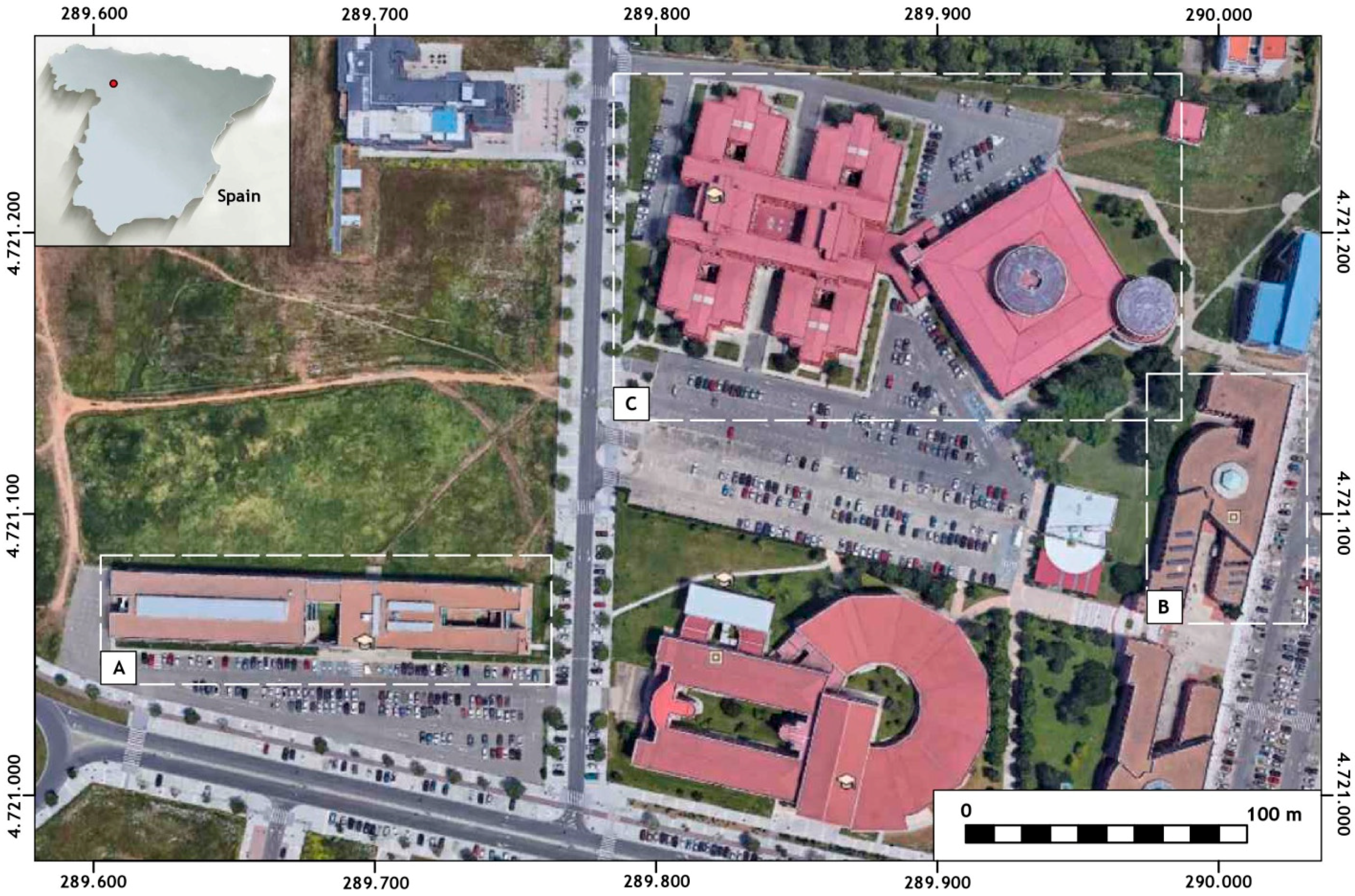
The different heating options contemplated in this work were designed to cover the thermal needs of three buildings placed at the University Campus of Vegazana in the province of León (Spain):
- The university school of education (A)
- The higher and technical school of mining engineers (B)
- The higher and technical school of industrial and aerospace engineering (C)
Figure 1 shows the regional situation and location of the buildings in question.
The present heat source that covers the thermal demand of these universities is a common installation of natural gas where each building is supplied by an individual boiler. The annual use of fuel of each construction can be found in Table 1. Additional information is provided in Table A1 of Appendix A.
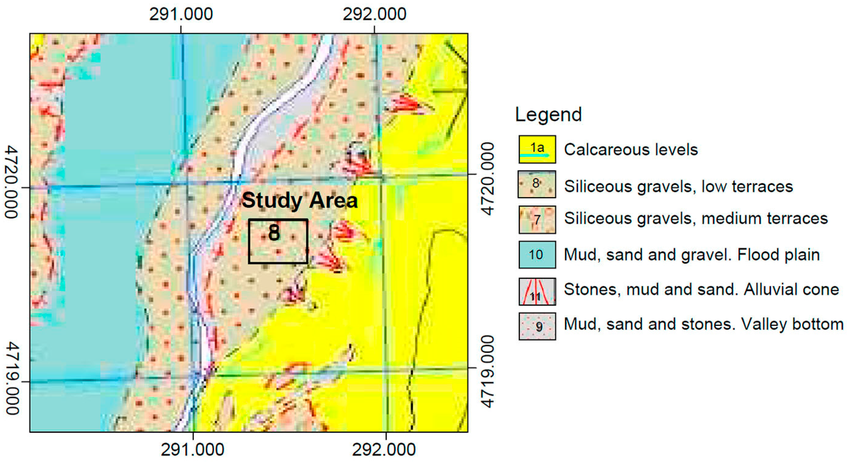
Figure 2 shows the geological characterization of the area where the research is set. The geological formations play a fundamental role in the process of thermal exchange between ground and the heat carrier fluid. For this reason, geology is subsequently required during the process of calculation of the future geothermal district heating system. Parameters such as the total drilling length or the heat pump power are closely related to the capacity of the ground to conduce the heat (thermal conductivity of the ground). Table 2 presents the parameter of thermal conductivity for each of the geological formations described in Figure 2.
Additionally, the meteorological information of the study area is presented in Table A2 belonging to Appendix A.
2.2. Description of the Proposed Solutions
● Case 1
The first alternative was designed to cover the thermal needs of the set of buildings by a district heating system exclusively aided by geothermal energy. The integrated installation was defined to supply the thermal demand of each of the buildings connected to the network. The generator plant was constituted by a vertical closed-loop geothermal system of very low enthalpy since the drilling depths (as Section 3.1 shows) are moderate. Additionally, the geological characteristics of the area in question did not allow implementing any other version of geothermal energy, given that high temperature points are not found in that kind of materials.
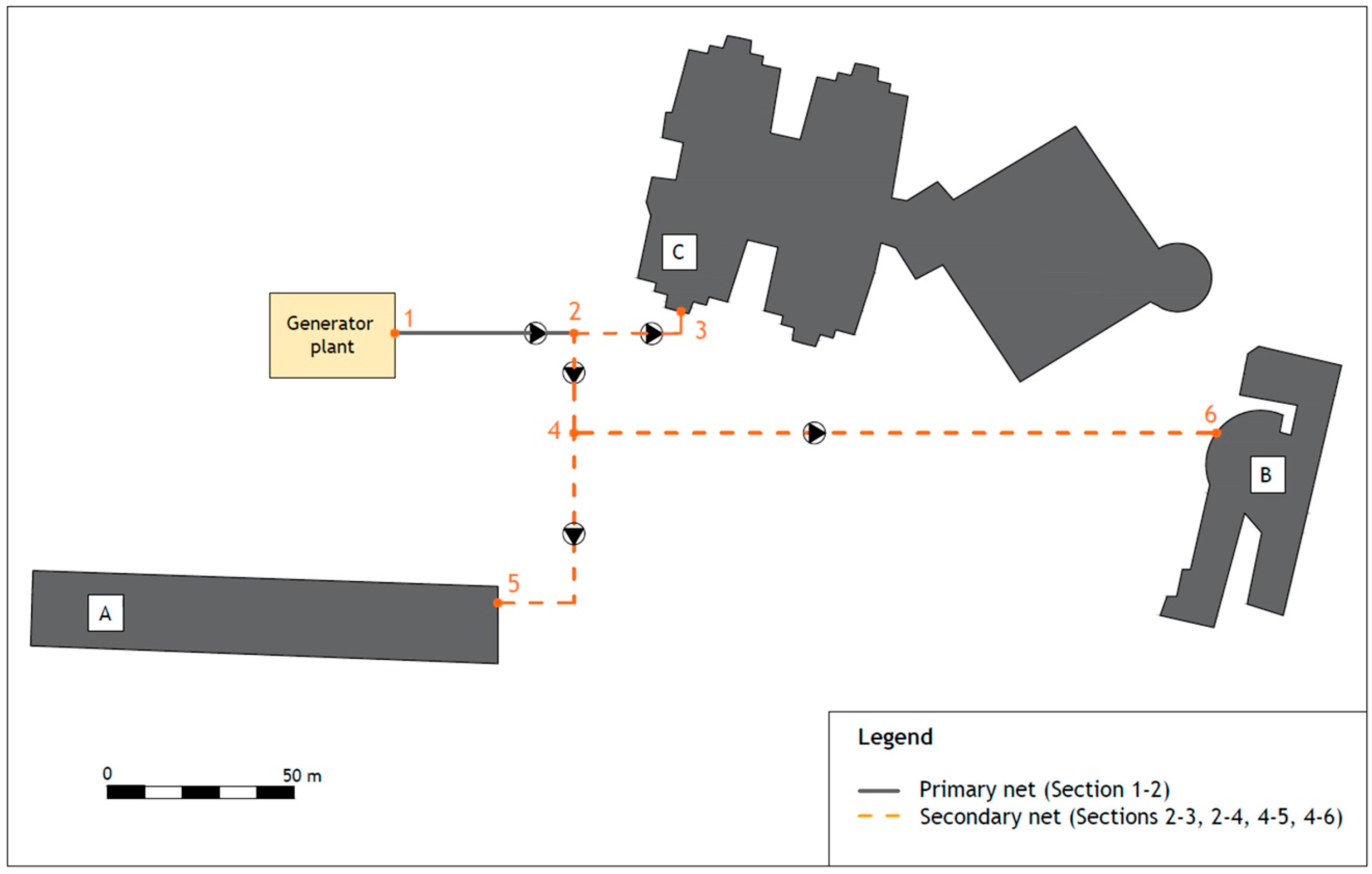
The central installation was planned to follow a branched pattern (fishbone schema) where each building was connected to the same generator plant by a single supplying network. The structure of the fishbone schema can be found in Figure 3. This figure presents an initial schema of the primary and secondary nets that constitutes the projected district heating plant.
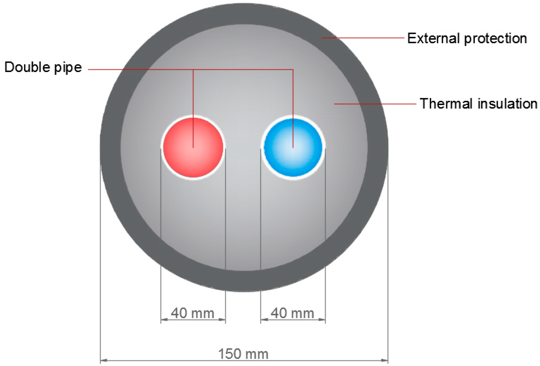
Since it was designed to just cover the heating needs, the circuit consisted of a double pipe pattern. In this system, one of the pipes is responsible for transporting the fluid to each building which returns through a second pipe to the main plant. Both pipes were properly insulated and protected, as Figure 4 shows.
● Case 2
The second solution to supply the demand of the buildings in question was projected to combine the geothermal district heating considered above and the existing natural gas installation. Thus, it was possible to reduce the total drilling length as well as the heat pump power of the geothermal plant. In this case the thermal demand was fundamentally covered by the geothermal district heating while the individual natural gas system (already existing) provided the remaining needs. The design of the geothermal district heating was identical to the one presented for case 1. However, the calculation of this option must be carried out independently.
● Case 3
The third assumption is quite similar to the above presented. However, this case proposes a district heating system where the generator plant is constituted by a single natural gas boiler in addition to the geothermal plant. Thus, the distribution system is common for both thermal sources. The geothermal system covers most of the total thermal demand (as in the previous case 2) while the natural gas boiler supplies the remaining demand. As it will be described in subsequent sections, the initial investment will be higher than in the previous case where the fossil installation is already set. Nevertheless, the higher efficiency of this natural gas boiler (in comparison with the individual heaters) will contribute to decrease the global operational costs.
Although cases 2 and 3 use as auxiliary energy source the natural gas, both cases present important differences. While case 2 need an individual natural gas boiler for each building, case 3 only implements a natural gas heater that will be common for the set of buildings.
2.3. Test Procedure
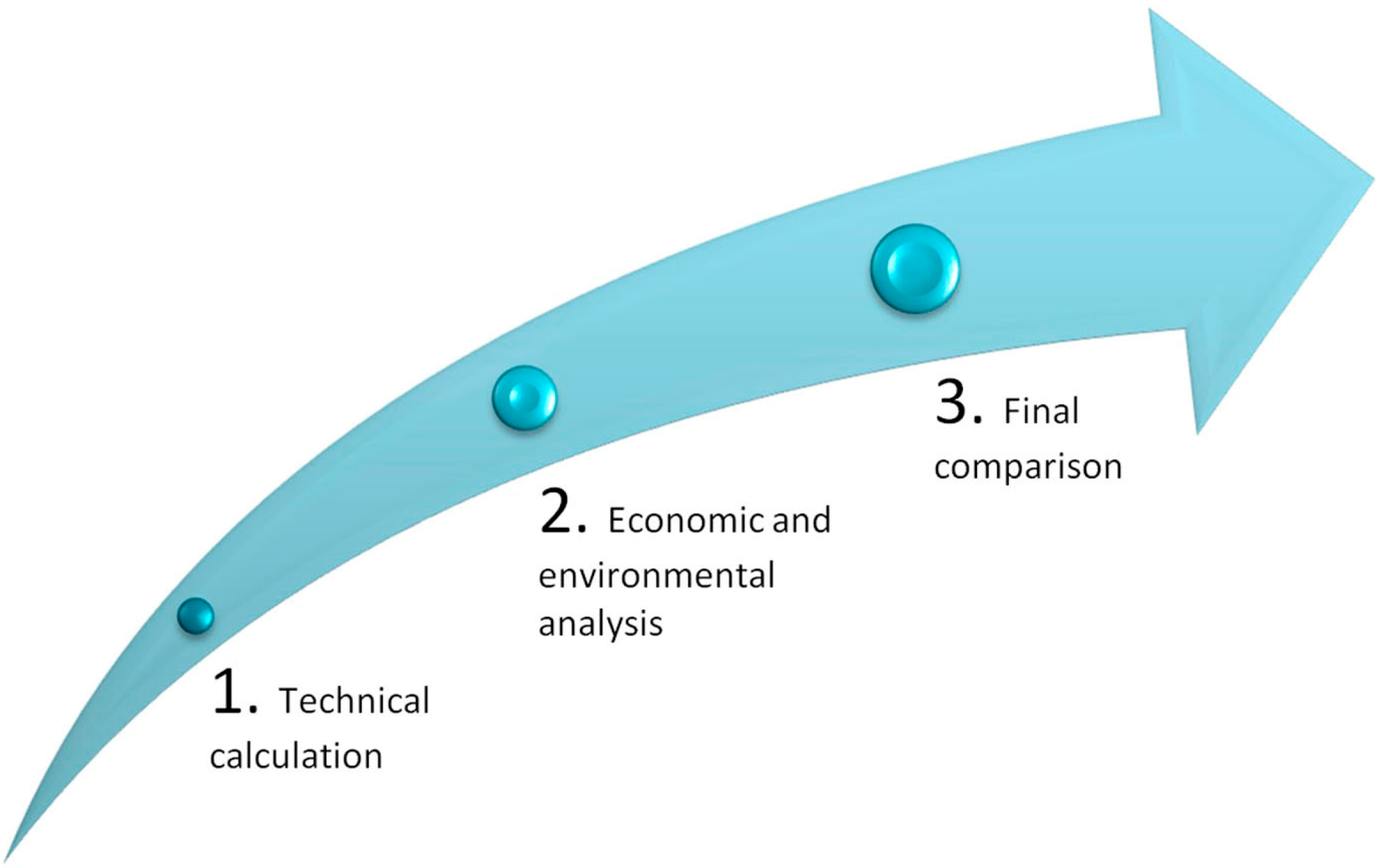
Initially, the proposed solutions previously described were technically calculated. The dimensioning of the district heating system derived from the thermal and geological description presented in the above section. Afterwards, an economic analysis of each option was also established. Once known this information, the proposed solutions (case 1, 2 and 3) and the existing installation were properly compared and evaluated. By way of clarification, the following Figure 5 describes the workflow followed throughout this research.
3. Results
3.1. Dimensioning
● Case 1 calculation
The dimensioning process of a district heating system involves the calculation of three main sections: the generator plant, the distribution system and the substations. Geothermal energy was in this case selected as the energy source to constitute the generator plant. By using the energy demand of the set of buildings integrating the district heating, the geothermal installation was calculated by the software “Earth Energy Designer” (EED). This software, developed by Blocon Software (Lund, Sweden), allows knowing the total drilling depth of the vertical closed-loop system and the heat pump power required in the plant. The calculation process of EED is based on a series of initial data (provided by the user) about the installation and the ground where it will be placed [26,27,28]. These initial data include the selection of the heat exchangers design. For this research, double-U polyethylene pipes of 32 mm in diameter, will allow the thermal exchange with the ground.
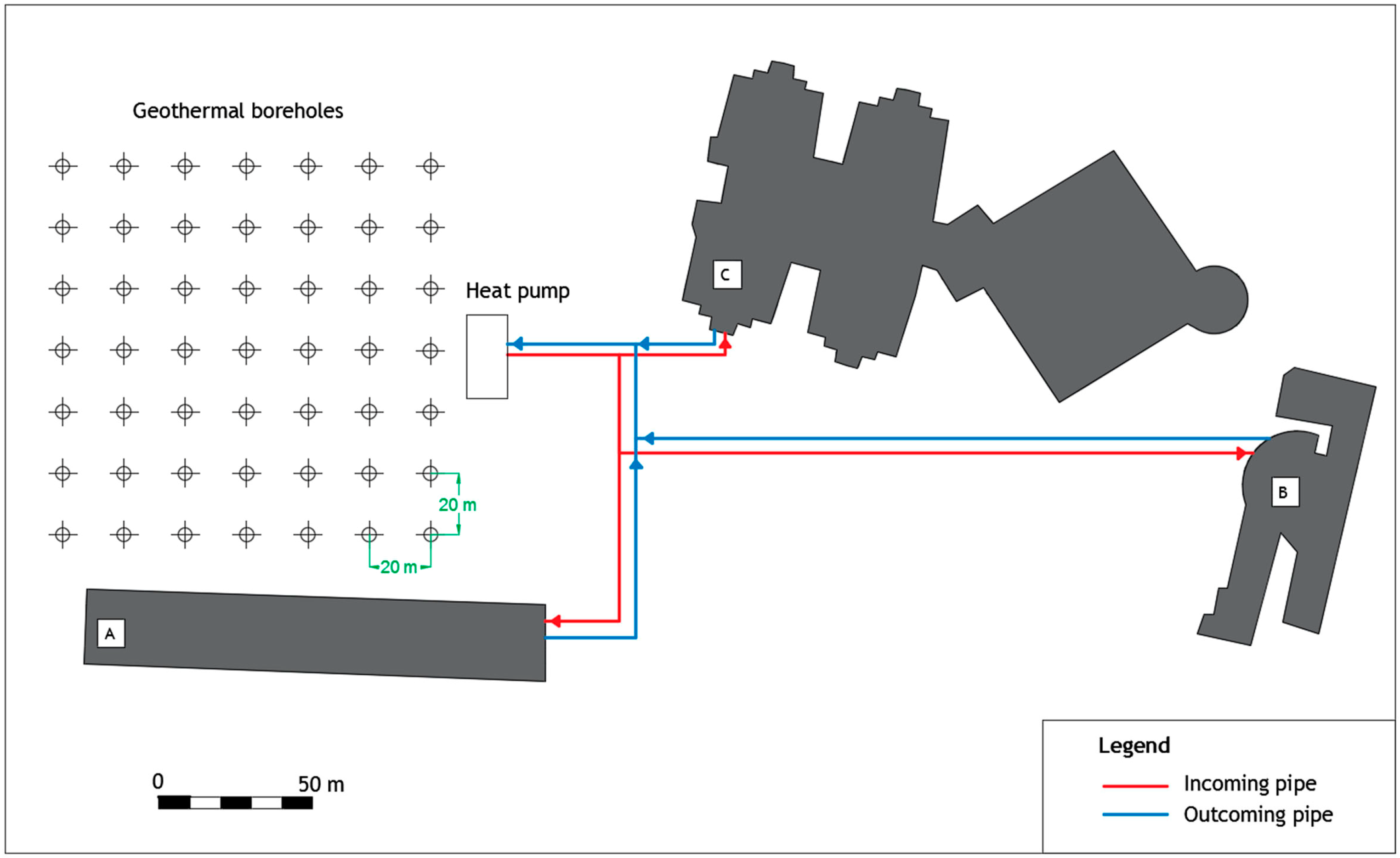
Once introduced the particular data of the system in question, EED evaluates the main parameters of the geothermal installation. In this way, the heat pump power and the number and length of boreholes required to cover the specific demand were calculated. During the process of calculation, the software suggests a series of alternatives. For the present assumption, the most optimal option (the first one) was selected so the installation requires a heat pump power of at least 330.62 kW and 49 boreholes of 178 m depth spaced every 20 m. The general distribution of each of the components of the geothermal district heating is presented in Figure 6.
By the above calculations, the part of the system corresponding to the geothermal installation (generator plant) was completely defined.
In relation to the distribution system, it was designed as a double-pipe system connecting the generator plant with each building. As made in the generator plant, this section was also thoroughly established. The diameters of the pipes were defined according to the mass flow rate. The required mass flow rate was calculated using Equation (1):
where: = mass flow rate (kg/s), = Capacity (kW), = temperature difference (K) and = specific heat capacity (kJ/kgK).
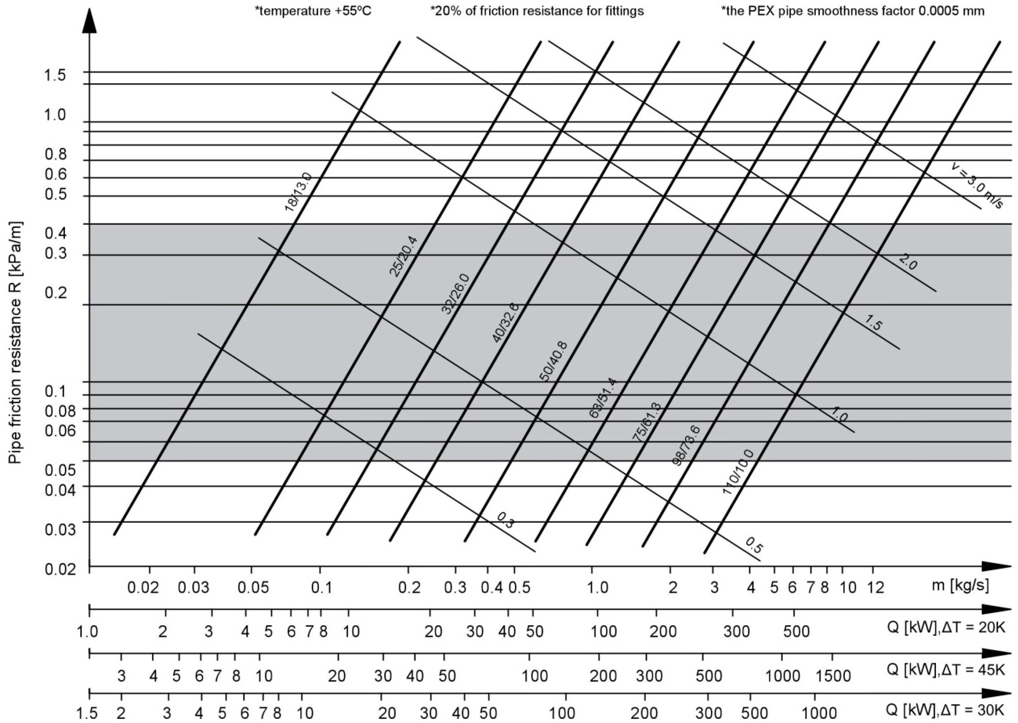
Considering PEX-a pipes, it was possible to observe at the nomogram of Figure 7 the recommended pressure loss area (in darker colour) for this kind of pipes. This nomogram allows knowing the diameter of piping required in function of the power installed and the expected thermal increase. On the basis of these data, the pipe diameter (mm), pipe friction resistance (kPa/m) and velocity (m/s) are directly deduced.
Entering in the nomogram the power installed in each section, the diameters of each pipe were directly obtained. The pipe friction resistances and velocities corresponding to those pipes were also established. Table 3 lists the descriptions of each section of pipe.
It must be clarified that the total power installed (section 1–2) should be 330.62 kW according to the calculations presented above. However, it is not possible to find commercial heat pumps with that exact power. Thus, the most similar commercial power was the 360 kW listed in Table 3.
Another important aspect to be considered is the heat loss through the pipes previously selected. They were accordingly calculated from the thermal transmittance provided by the manufacturer for each pipe diameter (considering pipes mounted in the air). These calculations can be found in Table A3 of Appendix A. Heat losses results are obtained for each section by the product of the thermal transmittance, the piping length and the thermal increase. The thermal increase considered in this Table A3 (80 K) represents the maximum increase that could be achieved in the system conditions for which the maximum heat losses would be found. Since the total losses are fewer than 3%, they have not been considered for subsequent calculations.
Substations were the last modules to be defined. They must be integrated by a set of heat exchangers, a buffer tank and different regulation and control devices. The buffer tank is responsible for adjusting the temperature and pressure conditions of the fluid coming from the generator plant. Its capacity was defined according to the “Regulation of thermal installations in buildings” (RITE) [30], which recommends a volume of 15–30 litres per kW of usable nominal power generated. Additionally, heat exchangers connect the generator plant with the primary circuit as well as the primary circuit with the rest of secondary nets. These systems were selected in function of the power installed in the section where they are placed. All of them were designed to work with the following conditions (Table 4):
● Case 2 calculation
The process of calculation of the geothermal district heating in this second case was equally performed by using the EED software. In the present option, the 70% of the whole demand (demands of buildings presented in Table 1) is covered by the renewable part of the mixed system (geothermal district heating). Therefore, entering in the software with the pertinent demand and the rest of specific values of the ground and installation, new working conditions were obtained. Thus, a heat pump power of 229.38 kW was needed and 36 boreholes of 193 m depth spaced every 24 m were required.
The same methodology than in the previous assumption was also applied to define the distribution system and substations in case 2. Given that the system of piping is identical, Equation (1) and nomogram presented in Figure 7 were also used to define the main parameters of each section of piping. These parameters can be found in Table 5.
Substations are constituted by the same elements described in case one. A buffer tank was also selected in this second option with a lower capacity since the total power was also lower. Relative to heat exchangers, they were designed to operate with the conditions previously collected in Table 4. The selection of these devices was also made depending on the power installed in each section.
Lastly, the remaining 30% of the global demand was covered by the set of individual natural gas boilers placed in each of the buildings. Thus, additional calculations were not needed given that the mentioned heaters were already installed and operating.
● Case 3 calculation
The generator plant was in this case planned to be constituted by a geothermal system and a sole natural gas heater. The geothermal plant was identical to the one calculated above for case 2 (since it covers the 70% of the demand too). Regarding the natural gas boiler, considering and efficiency of 0.9 (higher than the existing devices), to cover the 30% of the current demand (obtained from the consumptions of Table 1), a heater device of at least 218.9 kW would be needed. Thus, three commercial natural gas heaters of 80 kW (each one) were chosen providing enough power to supply the requested demand.
In relation to the distribution system and substations, they were designed to transport the whole power produced in the generator plant. Since the total distributed power was the same than in case one, the dimensioning process was identical and therefore parameters were those presented in Table 3 and Table 4. Therefore, piping, buffer tank and heat exchangers were the same than in case one.
3.2. Economic Analysis
Along this subsection an economic calculation is presented for each of the assumption considered in this research. This analysis includes the initial investment and operational costs as can be seen below.
3.2.1. Initial Investment
● Case 1
Once the first case was designed, it was possible to calculate the initial investment required. Table 6 presents the unitary and the total price of each of the components of the generator plant, distribution system and substations that are part of the geothermal district heating. Additionally, the total investment for this assumption is also collected in Table 6.
● Case 2
As in the first option, the initial investment was calculated as follows: regarding the natural gas installation, and given that it already exists, the initial costs of this part of the mixed system are zero. For this reason, the initial investment corresponding to the second case only includes the elements required in the geothermal district heating. Thus, the same elements of the previous option were also considered in this second assumption. Table 7 presents the initial investment of the mentioned elements belonging to the geothermal district heating of the second option.
● Case 3
The initial investment for case three includes the costs associated to the general district heating system. On this matter, the investment of the generator plant must consider the implementation of the geothermal module and the natural gas boiler. The costs connected to the distribution system and substations were identical to those calculated in case one. Table 8 collects the initial investment that case three involves.
3.2.2. Operational Costs
● Case 1
Despite being a completely renewable installation, in addition to the initial investment, several additional costs have to be considered. Such costs mainly correspond to the heat and circulating pump operation and the periodic installation maintenance.
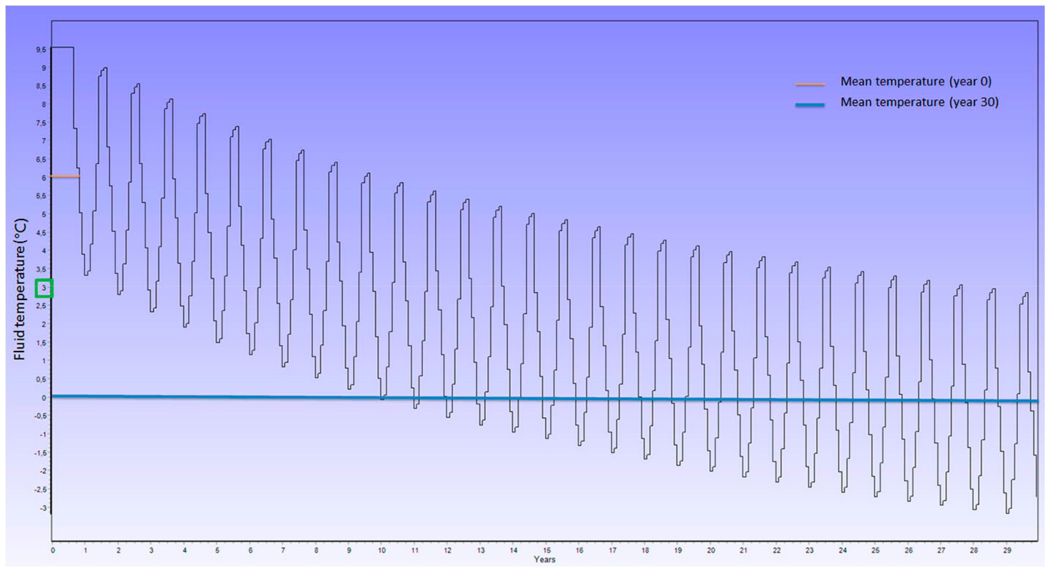
Most of the energy consumption derives from the heat pumps working. The excellent coefficient of operation (COP) of these devices allows them to provide a notable quantity of thermal energy consuming a minor amount of electricity. For the present case, two heat pumps of 180 kW (produced by ENERTRES, Galicia, Spain) connected in series provide a total of 360 kW that thoroughly cover the demand of 330.62 kW previously calculated. According to the manufacturer’s data, the power consumption of each of these devices is 40.92 kW, given the high COP (4.27) they have. This COP was calculated from the mean temperature of the fluid simulated with EED software for a thirty years operational period. From this simulation presented in Figure 8, the mean temperature of the fluid (3 °C) was estimated in order to obtain the mentioned COP for that period and according to the European Normative UE 813/2013 [31].
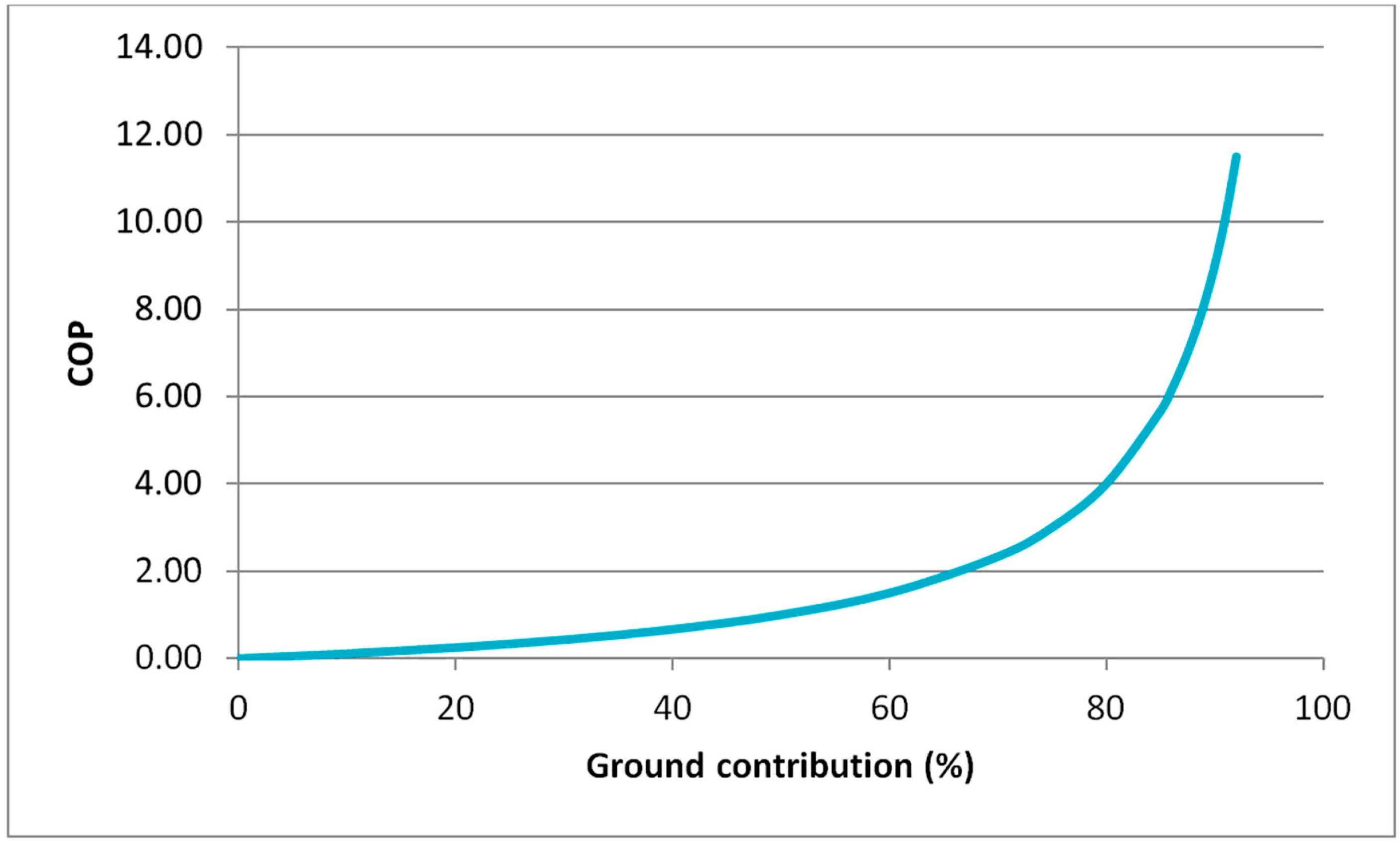
Heat pumps will be operational during 9 months a year for an average of 10 h a day (considering the climatic conditions of the area and the use of the buildings). It means an electrical use of 220.968 kWh/year for the set of geothermal heat pumps. It is important to clarify that the high seasonal COP is possible thanks to a combination of different factors. The heat pumps connection (in series) increases the COP of the second heat pump, this fact joined to the favourable geological and hydrogeological ground conditions result in an improvement of the global COP. Additionally, the ground/heat pump contribution ratio shoots up the COP with a small ground contribution increase. This fact can be observed in Figure 9.
Since the electrical use of the rest of components that integrate the geothermal district heating was comparatively lower, in this section, only the heat pumps consumption and the maintenance of the whole installation were considered. Table 9 provides the costs associated to the mentioned items.
● Case 2
The operational costs in this case derive from the heat pumps operation and maintenance of the whole district heating system as well as the fossil installation working. Regarding the geothermal plant, two heat pumps (of 90 kW and 140 kW) connected in series provide 230 kW to supply the previously calculated power of 229.38 kW. The COP of these pumps is also extraordinary (of 4.27 and 4.33 respectively) and hence, the power consumptions of these devices are 20.46 kW and 32.76 kW. These COP values were equally calculated as in the previous case 1. Likewise, heat pumps will be operational during 9 months a year to an average of 10 h a day. Thus, the electricity use of both heat pumps will be of 143.694 kWh/year. As in the previous case, the electricity use of the rest of components of the geothermal district heating was not considered (since it is comparatively lower).
Thanks to the geothermal system, the 70% of the total demand is covered. The remaining demand is provided by the existing fossil installation. For this reason, the operational costs must also include the pertinent natural gas use. Table 10 collects the operational costs including all the mentioned items.
● Case 3
In this last case, operational costs include the district heating working which, in turn, involves the heat pumps and natural gas heater operation besides the maintenance of the whole general system.
Since the geothermal plant was designed to cover the same demand than in case two (70% of the total demand), heat pumps described in that case are also used here. Thus, a power consumption of 143.694 kWh/year is required to supply two heat pumps of 90 kW and 140 kW. Natural gas use of the heater that integrates the generator plant must be also considered in this section. As in the previous case, operational costs for the natural gas are calculated considering the natural gas use (kW/h) and a local rate of 0.056 €/kWh + 4.54 €/month.
Table 11 shows the operational cost corresponding to case three.
3.3. Environmental Analysis
The environmental analysis is performed according to the CO2 emissions associated with each scenario. The estimation of the greenhouse gases is based on a series of emission factors commonly accepted for each of the energy sources used [32]. Thus, Table 12 presents the quantity of CO2 emitted by the installations implemented in each of the cases described in the manuscript. It is important to clarify that for case 1, CO2 emissions are the corresponding to the heat pumps operation. For case 2, emissions are associated to the heat pumps working as well as the fossil installation. For case 3, these emissions derive from the operation of the heat pumps and the unique natural gas boiler. Therefore, for cases 2 and 3, two conversion factors are considered. Finally, CO2 emissions of the system currently installed (designated here as case 4) correspond to the fossil plant constituted by three individual natural gas devices.
4. Discussion
Three different scenarios have been described in the present manuscript. These options together with the existing fossil installation (case 4) are now evaluated and compared from an economic and environmental point of view.
Table 13 presents the economic balance based on the calculations made in the above section. The comparison considers the initial investment and operational costs per year of each assumption until a period of thirty years (lifespan of these plants). With the aim of updating the costs of each year to the real value in that moment, data are express in terms of the “Net Present Value” (NPV). Equation (2) shows the expression for NPV:
where: I0 = Initial investment, C1 = Operational costs for year 1, C2 = Operational costs for year 2, CT = Operational costs for year T and k = Discount rate.
Every term of Equation (2) is negative given that initial investment and operational costs are both outlays and there are no positive cash flows. Additionally, it must be mentioned that a discount rate of 1.8% has been used in all the calculations. The operational costs for case 4 presented in this Table 13, are exclusively those corresponding to the use of natural gas.
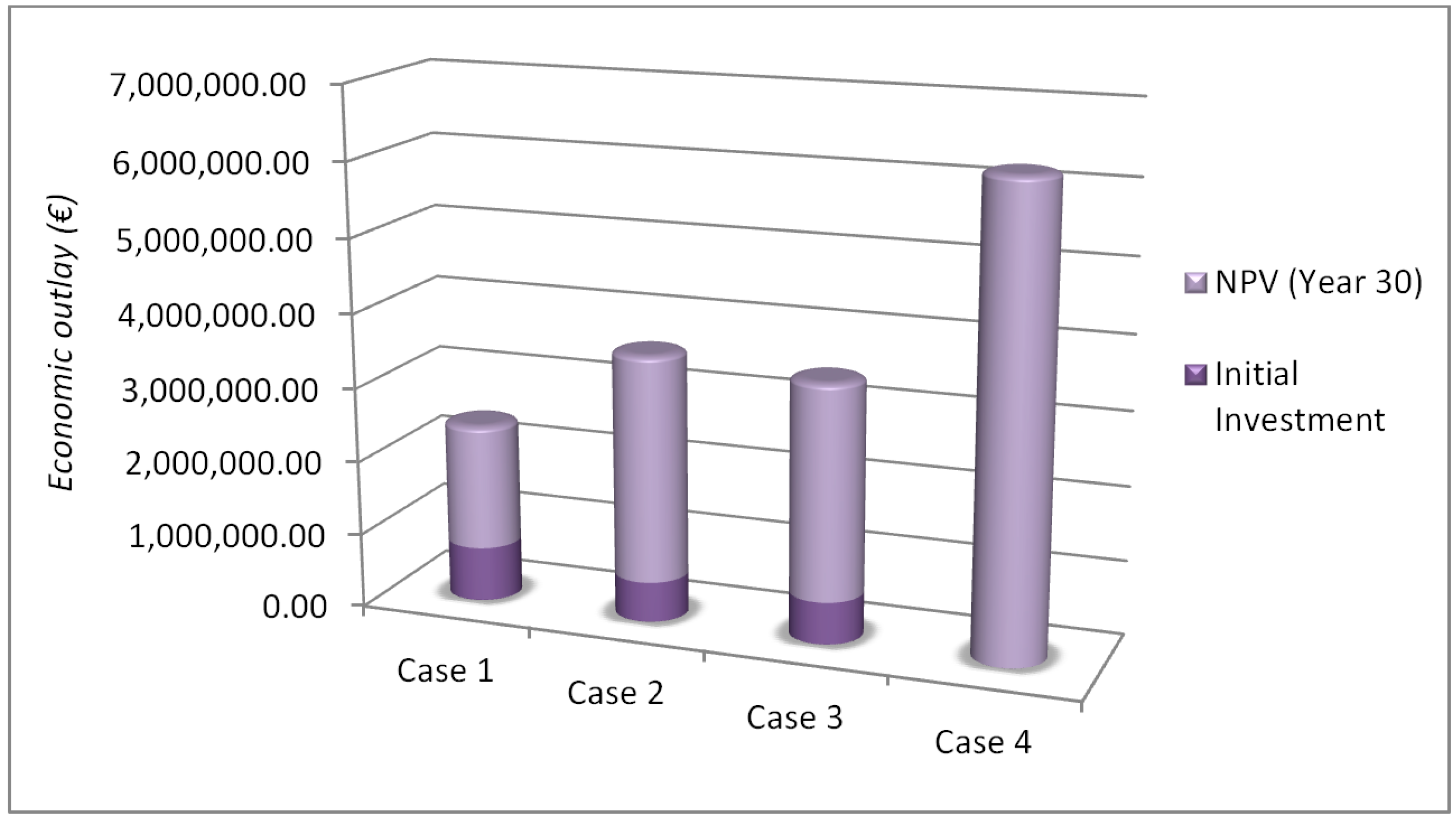
Figure 10 graphically shows the final economic results presented in the above Table 13 at the end of the period considered.
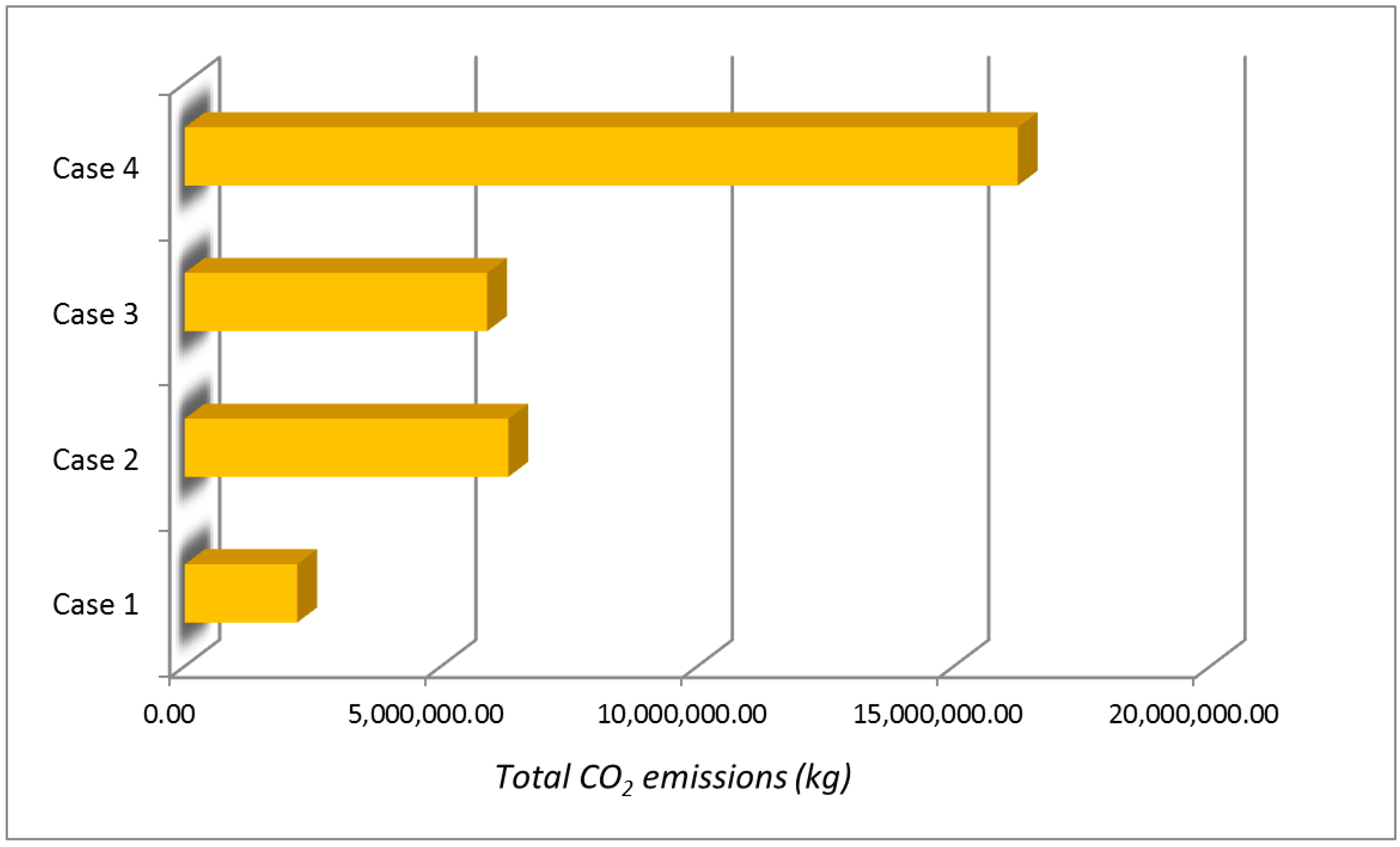
At same time, from the annual environmental analysis previously presented in Section 3.3, it was possible to estimate the total CO2 emissions accumulated at the end of the period considered (year 30). In this way, Figure 11 schematically shows the mentioned parameter for each of the cases described in this study. From the economic and environmental comparisons expounded above, a series of statements can be made:
- The first option (case 1) requires the highest initial investment in contrast with the existing system (case 4) where this item is null. Regarding the initial investment of cases 2 and 3 (quite similar), it is significantly lower (around 25%) than in case 1.
- Analysing the operational costs, it is easily observable that case 4 has the highest costs due to the plant working in each one of the years considered. On the contrary, the lowest operational costs belong to case 1, with case 2 and 3 in the middle of both scenarios.
- Differences of operational costs between cases 1 and 4 progressively increase until year 30 where the maximum deviation is found. Thus, the high initial investment of case 1 would be more than amortized in the eighth year in comparison with the present installation (case 4). Case 2 and 3 would also be amortized in year 8. However, the total savings in the last year (year 30) are much more favourable for case 1.
- In economic terms, and considering the global balance of Table 13 named “NPV”, the most favourable option is case 1, followed by case 3 and case 2. From an economic point of view these assumptions (case 2 and 3) are quite similar and significant differences are not detected. On the other hand, case 4 is clearly distanced from the rest of scenarios constituting the worst option regarding the economic issue.
- In respect of the environmental point of view, case 1 involves the lowest quantity of annual CO2 emissions. In case 2 and 3 these emissions are of around three times larger than in the first assumption. Regarding case 4, CO2 emissions are seven times larger than in case 1. Therefore, with reference to the environmental aspect, case 1 represents the most respectful and appropriate solution for the area studied in this research. At the other extreme, case 4 constitutes the least favourable option given the high level of CO2 emissions its operation involves.
5. Conclusions
An exhaustive calculation of three options specifically designed to cover the thermal needs of a set of buildings has been carried out in this study. From these calculations, an economic and environmental analysis has been presented in order to compare the different scenarios and select the most suitable one. Based on this comparison, case 1, where a geothermal district heating is proposed, means the ideal solution from both the economic and environmental point of view. Although it requires the highest initial investment, the operational costs are significantly lower than in the current fossil system and in the rest of cases studied. Thus, the investment would be easily amortized in a short period of time and important savings could be achieved in the remaining lifetime of the system in question. Additionally, this case 1 is also supported by the environmental side since it presents the lowest CO2 emission rate. Even the mixed systems (case 2 and 3) constituted by geothermal energy and natural gas heaters are substantially better than the existing fossil installation thanks to the introduction of the mentioned renewable source. In any case, it has been demonstrated how the use of the geothermal energy offer a large number of interesting advantages. The initial investment of this kind of geothermal plants is always amortized in the first years of operation. In addition, the scarce electricity demand of the geothermal heat pumps causes the low operational costs as well as a limited greenhouse gases emission.
Author Contributions
All authors conceived, designed and performed the experimental and theoretical basis of the research. C.S.B., A.F.M. and I.M.N. implemented the methodology and calculations and analysed the results. D.G.-A. provided technical and theoretical support. C.S.B. wrote the manuscript and all authors read and approved the final version.
Acknowledgments
Authors would like to thank the Department of Cartographic and Land Engineering of the Higher Polytechnic School of Avila, University of Salamanca, for allowing us to use their facilities and their collaboration during the experimental phase of this research. The gratitude is extensible to the University of León for providing the real data used in this work. Authors also want to thank the Ministry of Education, Culture and Sport for providing a FPU Grant (Training of University Teachers Grant) to the corresponding author of this paper what has made possible the realization of the present work.
Conflicts of Interest
The authors declare no conflict of interest.
Appendix A

Table A1.
Additional characterization of the buildings studied.
| Building | Total heated Surface (m2) | Usual Number of Occupants | Operational Schedule |
|---|---|---|---|
| A | 4914.09 | 148 | 9 months/year Mean value of 10 hours/day |
| B | 3402.39 | 102 | |
| C | 13,096.88 | 393 |
Table A2.
Meteorological information of the place where the study is focused.
| Month. | Mean Temperature (°C) | Minimum Temperature (°C) | Maximum Temperature (°C) |
|---|---|---|---|
| January | 3.2 | −0.7 | 7.1 |
| February | 4.6 | 0 | 9.3 |
| March | 7.6 | 2.6 | 12.7 |
| April | 9.7 | 3.8 | 15.6 |
| May | 12.6 | 6.5 | 18.8 |
| June | 17.1 | 10.1 | 24.2 |
| July | 19.7 | 11.8 | 27.7 |
| August | 19.5 | 12 | 27 |
| September | 16.7 | 10 | 23.4 |
| October | 11.9 | 6.3 | 17.6 |
| November | 7.3 | 2.7 | 12 |
| December | 4.2 | 0.6 | 7.9 |
Table A3.
Power losses of each section of pipes and total loss for the set of piping.
| Section | Length (m) | ∆T (K) | Thermal Transmittance (W/mk) | Power Loss * (kW) | Power Flow (kW) | Loss (%) |
|---|---|---|---|---|---|---|
| 1–2 | 36.72 | 80 | 0.40 | 1.17 | 360.00 | 0.33 |
| 2–3 | 41.29 | 80 | 0.38 | 1.25 | 239.40 | 0.52 |
| 2–4 | 32.11 | 80 | 0.34 | 0.69 | 120.60 | 0.57 |
| 4–5 | 79.04 | 80 | 0.32 | 2.02 | 76.28 | 2.65 |
| 4–6 | 206.53 | 80 | 0.32 | 5.29 | 44.32 | 11.93 |
| Total loss | 10.42 | 360.00 | 2.89 | |||
* Calculated from the product of Length, temperature increment and thermal transmittance.
References
- Carotenuto, A.; Figaj, R.D.; Vanoli, L. A novel solar-geothermal district heating, cooling and domestic hot water system: Dynamic simulation and energy-economic analysis. Energy 2017, 141, 2652–2669. [Google Scholar] [CrossRef]
- Mink, L.L. The Nation’s Oldest and Largest Geothermal District Heating System. Geotherm. Resour. Counc. Trans. 2017, 41, 205–212. [Google Scholar]
- Oktay, Z.; Coskun, C.; Dincer, I. Energetic and exergetic performance investigation of the Bigadic Geothermal District Heating System in Turkey. Energy Build. 2008, 40, 702–709. [Google Scholar] [CrossRef]
- Pinto, J.F.; da Graça, G.C. Comparison between geothermal district heating and deep energy refurbishment of residential building districts. Appl. Therm. Eng. 2007, 27, 1303–1310. [Google Scholar]
- Arat, H.; Arslan, O. Exergoeconomic analysis of district heating system boosted by the geothermal heat pump. Energy 2017, 119, 1159–1170. [Google Scholar] [CrossRef]
- Unternährer, J.; Moret, S.; Joost, S.; Maréchal, F. Spatial clustering for district heating integration in urban energy systems: Application to geothermal energy. Appl. Energy 2017, 190, 749–763. [Google Scholar] [CrossRef]
- Keçebaş, A.; Hepbasli, A. Conventional and advanced exergoeconomic analyses of geothermal district heating systems. Energy Build. 2014, 69, 434–441. [Google Scholar] [CrossRef]
- Kyriakis, S.A.; Younger, P.L. Towards the increased utilisation of geothermal energy in a district heating network through the use of a heat storage. Appl. Therm. Eng. 2016, 94, 99–110. [Google Scholar] [CrossRef]
- Lund, J.W.; Boyd, T.L. Direct utilization of geothermal energy 2015 worldwide review. Geothermics 2016, 60, 66–93. [Google Scholar] [CrossRef]
- Hepbasli, A.; Canakci, C. Geothermal district heating applications in Turkey: A case study of Izmir–Balcova. Energy Convers. Manag. 2003, 44, 1285–1301. [Google Scholar] [CrossRef]
- Abdurafikov, R.; Grahn, E.; Ypyä, L.K.J.; Kaukonen, S.; Heimonen, I.; Paiho, S. An analysis of heating energy scenarios of a Finnish case district. Sustain. Cities Soc. 2017, 32, 56–66. [Google Scholar] [CrossRef]
- Carotenuto, A.; De Luca, G.; Fabozzi, S.; Figaj, R.D.; Iorio, M.; Massarotti, N.; Vanoli, L. Energy analysis of a small geothermal district heating system in Southern Italy. Int. J. Heat Technol. 2016, 34, S519–S527. [Google Scholar] [CrossRef]
- Sander, M. Geothermal district heating systems: Country case studies from China, Germany, Iceland, and United States of America, and schemes to overcome the gaps. Trans. Geotherm. Resour. Counc. 2016, 40, 769–775. [Google Scholar]
- Muñoz, M.; Garat, P.; Flores-Aqueveque, V.; Vargas, G.; Rebolledo, S.; Sepúlveda, S.; Daniele, L.; Morata, D.; Parada, M.Á. Estimating low-enthalpy geothermal energy potential for district heating in Santiago basin-Chile (33.5 °S). Renew. Energy 2015, 76, 186–195. [Google Scholar] [CrossRef]
- Soltero, V.M.; Chacartegui, R.; Ortiz, C.; Velázquez, R. Evaluation of the potential of natural gas district heating cogeneration in Spain as a tool for decarbonisation of the economy. Energy 2016, 115, 1513–1532. [Google Scholar] [CrossRef]
- Rodriguez-Aumente, P.A.; del Carmen Rodriguez-Hidalgo, M.; Nogueira, J.I.; del Carmen Venegas, M. District heating and cooling for business buildings in Madrid. Appl. Therm. Eng. 2013, 50, 1496–1503. [Google Scholar] [CrossRef]
- Ioakimidis, C.S.; Gutiérrez, I.A.; Genikomsakis, K.N.; Stroe, E.R.; Savuto, E. The use of district heating on a small Spanish village. In Proceedings of the 26th International Conference on Efficiency, Cost, Optimization, Simulation and Environmental Impact of Energy Systems, ECOS, Guilin, China, 19 July 2013. [Google Scholar]
- Ozgener, L.; Hepbasli, A.; Dincer, I.; Rosen, M.A. Exergoeconomic analysis of geothermal district heating systems: A case study. Appl. Therm. Eng. 2007, 27, 1303–1310. [Google Scholar] [CrossRef]
- Möller, B.; Lund, H. Conversion of individual natural gas to district heating: Geographical studies of supply costs and consequences for the Danish energy system. Appl. Energy 2010, 87, 1846–1857. [Google Scholar] [CrossRef]
- Keçebas, A. Performance and thermo-economic assessments of geothermal district heating system: A case study in Afyon, Turkey. Renew. Energy 2011, 36, 77–83. [Google Scholar] [CrossRef]
- Keçebaş, P.; Gökgedik, H.; Alkan, M.A.; Keçebaş, A. An economic comparison and evaluation of two geothermal district heating systems for advanced exergoeconomic analysis. Energy Convers. Manag. 2014, 84, 471–480. [Google Scholar] [CrossRef]
- Hepbasli, A.; Keçebaş, A. A comparative study on conventional and advanced exergetic analyses of geothermal district heating systems based on actual operational data. Energy Build. 2013, 61, 193–201. [Google Scholar] [CrossRef]
- Aslan, A.; Yüksel, B.; Akyol, T. Energy analysis of different types of buildings in Gonen geothermal district heating system. Appl. Therm. Eng. 2011, 31, 2726–2734. [Google Scholar] [CrossRef]
- Ministerio de Economía. Industria y Competitividad; Instituto Geológico y Minero de España (IGME): Madrid, Spain, 2003. [Google Scholar]
- Blázquez, C.S.; Martín, A.F.; Nieto, I.M.; García, P.C.; Pérez, L.S.S.; Aguilera, D.G. Thermal conductivity map of the Avila region (Spain) based on thermal conductivity measurements of different rock and soil samples. Geothermics 2017, 65, 60–71. [Google Scholar] [CrossRef]
- Sliwa, T.; Nowosiad, T.; Vytyaz, O.; Sapinska-Sliwa, A. Study on the efficiency of deep borehole heat exchangers. SOCAR Proc. 2016, 2, 29–42. [Google Scholar] [CrossRef]
- Blázquez, C.S.; Martín, A.F.; Nieto, I.M.; González-Aguilera, D. Measuring of Thermal Conductivities of Soils and Rocks to Be Used in the Calculation of A Geothermal Installation. Energies 2017, 10, 795–813. [Google Scholar] [CrossRef]
- Blázquez, C.S.; Martín, A.F.; García, P.C.; Pérez, L.S.S.; del Caso, S.J. Analysis of the process of design of a geothermal installation. Renew. Energy 2016, 89, 1–12. [Google Scholar] [CrossRef]
- Uponor. Guía de Microrredes de Distrito de Calor y Frío, 1st ed.; Uponor: Pfungen, Switzerland, 2011. [Google Scholar]
- Ministerio de Industria. Energía y Turismo, Dirección General de Política Energética y Minas, Reglamento de Instalaciones Térmicas en los Edificios (RITE); Ministerio de Industria: Madrid, Spain, 2013. [Google Scholar]
- European Commission. Reglamento (UE) 813/2013 de la Comisión de 2 de Agosto de 2013 por el que se Desarrolla la Directiva 2009/125/CE del Parlamento Europeo y del Consejo Respecto de Los Requisitos de Diseño Ecológico Aplicables a Los Aparatos de Calefacción y a los Calefactores Combinados; European Commission: Brussels, Belgium, 2013. [Google Scholar]
- Ministerio de Industria. Energía y Turismo, IDEA (Instituto Para la Diversificación y Ahorro de la Energía), Factores de Emisión de CO2 y Coeficientes de Paso a Energía Primaria de Diferentes Fuentes de Energía Final Consumidas en el Sector de Edificios en España; Ministerio de Industria: Madrid, Spain, 2014. [Google Scholar]
Figure 1.
Position of the buildings considered in the present research (Geodetic Datum: WGS84, Cartographic projection: UTM, Time zone: 30).
Figure 1.
Position of the buildings considered in the present research (Geodetic Datum: WGS84, Cartographic projection: UTM, Time zone: 30).

Figure 2.
Geological description of the study area [24].
Figure 2.
Geological description of the study area [24].

Figure 3.
Network distribution.

Figure 4.
Schema of the double pipe system of 40 mm in diameter.

Figure 5.
Workflow established in the present research.

Figure 6.
Schema of the main components of the whole geothermal district heating system.

Figure 7.
Nomogram of pipe friction resistance-flow-velocity for PEX-a pipes [29].
Figure 7.
Nomogram of pipe friction resistance-flow-velocity for PEX-a pipes [29].

Figure 8.
Fluid temperature evolution for the period of thirty years.

Figure 9.
Relation COP-Ground contribution.

Figure 10.
Economic position at the end of the period studied (thirty years).

Figure 11.
CO2 emissions associated to each scenario at the end of year 30.

Table 1.
Annual use of natural gas of each building.
| Building | Annual Use of Natural Gas (kWh) |
|---|---|
| University school of education (A) | 455,541.00 |
| Higher and technical school of mining engineers (B) | 264,666.00 |
| Higher and technical school of industrial and aerospace engineering (C) | 1,429,101.00 |
Table 2.
Thermal conductivity of the materials presented in the study area.
| Geological Formation | Thermal Conductivity (W/mK) * |
|---|---|
| Calcareous levels | 1.40 |
| Siliceous gravels | 0.80 |
| Mud, sand and stones | 1.10 |
| Mud, sand and gravel | 1.30 |
* Values based on laboratory measurements in materials with similar geological composition [25].
Table 3.
Main parameters of the pipes used in the geothermal district heating.
| Section * | Power Installed (kW) | Thermal Increase (K) | Flow Rate (L/h) | Velocity (m/s) | Pipe Friction Resistance (kPa/m) | Pipe Diameter (mm) |
|---|---|---|---|---|---|---|
| 1–2 | 360 | 20 | 15,480 | 1.59 | 0.34 | 75 |
| 2–3 | 239.40 | 20 | 10,292 | 1.25 | 0.22 | 63 |
| 2–4 | 120.60 | 20 | 5186 | 1.00 | 0.26 | 50 |
| 4–5 | 76.28 | 20 | 3280 | 1.10 | 0.37 | 40 |
| 4–6 | 44.32 | 20 | 1906 | 0.65 | 017 | 40 |
* Sections can be found in Figure 3.
Table 4.
Heat exchangers working conditions.
| Condition | Primary Circuit | Secondary Circuit (User) |
|---|---|---|
| Inlet temperature (°C) | Minimum 80 | Maximum 25 |
| Outlet temperature (°C) | Maximum 60 | Maximum 50 |
Table 5.
Main parameters of the pipes used in the case 2.
| Section | Power Installed (kW) | Thermal Increase (K) | Flow Rate (L/h) | Velocity (m/s) | Pipe Friction Resistance (kPa/m) | Pipe Diameter (mm) |
|---|---|---|---|---|---|---|
| 1–2 | 230 | 20 | 9890 | 1.20 | 0.24 | 63 |
| 2–3 | 152.95 | 20 | 6577 | 1.18 | 0.30 | 50 |
| 2–4 | 77.05 | 20 | 3313 | 1.10 | 0.39 | 40 |
| 4–5 | 48.74 | 20 | 2096 | 0.77 | 0.21 | 40 |
| 4–6 | 28.31 | 20 | 1217 | 0.60 | 0.20 | 32 |
Table 6.
Summary of the initial investment for case 1.
| Initial Investment Case 1 | ||||
|---|---|---|---|---|
| Element | Quantity | Unitary Price (€) | Total Price (€) | |
| Generator plant | Drilling | 8722 * | 44.00 | 383,768.00 |
| Heat pumps | 2 ** | 115,010.00 | 230,020.00 | |
| Heat exchangers | 49 ** | 880.00 | 43,120.00 | |
| Control device | 1 ** | 120.00 | 120.00 | |
| Accessory elements | - | - | 11,573.20 | |
| Distribution system | Double piping | 395.69 * | - | 35,048.19 |
| Circulating pumps | 5 ** | - | 8664.00 | |
| Leak detection system | 1 ** | 948.00 | 948.00 | |
| Accessory elements | - | - | 4712.58 | |
| Substation | Buffer tank | 1 ** | 10,700.00 | 10,700.00 |
| Heat exchangers | 3 ** | - | 2782.00 | |
| Total investment (€) | 731,455.97 | |||
* (meters), ** (units).
Table 7.
Summary of the initial investment for case 2.
| Initial Investment Case 2 | ||||
|---|---|---|---|---|
| Element | Quantity | Unit Price (€) | Total Price (€) | |
| Generator plant | Drilling | 6948 * | 44.00 | 305,712.00 |
| Heat pumps | 2 ** | 69,379.00 | 138,758.00 | |
| Heat exchangers | 36 ** | 880.00 | 31,680.00 | |
| Control device | 1 ** | 120.00 | 120.00 | |
| Accessory elements | - | - | 9196.80 | |
| Distribution system | Double piping | 395.69 * | - | 30,734.97 |
| Circulating pumps | 5 ** | 1678.80 | 8394.00 | |
| Leak detection system | 1 ** | 948.00 | 948.00 | |
| Accessory elements | - | - | 4712.59 | |
| Substation | Buffer tank | 1 ** | 6588.00 | 6588.00 |
| Heat exchangers | 3 ** | - | 2316.00 | |
| Total investment (€) | 539,160.36 | |||
* (meters), ** (units).
Table 8.
Summary of the initial investment for case 3.
| Initial Investment Case 3 | ||||
|---|---|---|---|---|
| Element | Quantity | Unitary Price (€) | Total Price (€) | |
| Generator plant | Drilling | 6948 * | 44.00 | 305,712.00 |
| Heat pumps | 2 ** | 69,379.00 | 138,758.00 | |
| Heat exchangers | 36 ** | 880.00 | 31,680.00 | |
| Control device | 1 ** | 120.00 | 120.00 | |
| Natural gas boiler | 3 ** | 4600.00 | 13,800.00 | |
| Accessory elements | - | - | 12,321.80 | |
| Distribution system | Double piping | 395.69 * | - | 35,048.19 |
| Circulating pumps | 5 ** | 1678.80 | 8664.00 | |
| Leak detection system | 1 ** | 948.00 | 948.00 | |
| Accessory elements | - | - | 4712.58 | |
| Substation | Buffer tank | 1 ** | 10,700.00 | 10,700.00 |
| Heat exchangers | 3 ** | - | 2782.00 | |
| Total investment (€) | 565,246.57 | |||
* (meters), ** (units).
Table 9.
Operational costs for case 1.
| Operational Costs Case 1 | |
|---|---|
| Item | Cost (€/year) |
| Heat pumps working | 28,725.84 * |
| District heating system maintenance | 3733.00 |
| Total operational costs | 32,498.84 |
* total cost per year for the two heat pumps required to cover the demand in question and considering a local rate of 0.13 €/kWh.
Table 10.
Operational costs for case 2.
| Operational Costs Case 2 | |
|---|---|
| Item | Cost (€/Year) |
| Heat pumps working | 18,680.22 * |
| District heating system and fossil plant maintenance | 4120.00 |
| Natural gas use | 36,147.72 ** |
| Total operational costs | 58,947.94 |
* total cost per year for the two heat pumps required to cover the 70% of the demand and considering a local rate of 0.13 €/kWh. ** Natural gas rate of 0.056 €/kWh + 4.54 €/month.
Table 11.
Operational costs for case 3.
| Operational Costs Case 3 | |
|---|---|
| Item | Cost (€/Year) |
| Heat pumps working | 18,680.22 * |
| District heating system maintenance | 3980.00 |
| Natural gas use | 33,138.82 ** |
| Total operational costs | 55,799.04 |
* total cost per year for the two heat pumps required to cover the 70% of the demand and considering a local rate of 0.13 €/kWh. ** Natural gas rate of 0.056 €/kWh + 4.54 €/month.
Table 12.
Conversion factor and emissions of CO2 for each assumption.
| Conversion Factor (kg CO2/kWh of Final Energy) | CO2 Emission (kg/Year) | |
|---|---|---|
| CASE 1 | 0.331 | 73,140.41 |
| CASE 2 | 0.331/0.252 | 210,374.59 |
| CASE 3 | 0.331/0.252 | 196,503.52 |
| CASE 4 | 0.252 | 541,602.94 |
Table 13.
Economic balance of each case for a period of 30 years.
| CASE 1 | CASE 2 | CASE 3 | CASE 4 | ||
|---|---|---|---|---|---|
| Initial Investment (€) | 731,345.38 | 539,055.45 | 565,135.98 | 0 | |
| OPERACIONAL COSTS (€) | Year 1 | 33,094.54 | 60,028.45 | 56,821.83 | 122,687.16 |
| Year 5 | 177,942.80 | 322,761.12 | 305,519.74 | 659,664.56 | |
| Year 10 | 389,720.26 | 706,893.15 | 669,132.04 | 1,444,760.01 | |
| Year 15 | 640,157.45 | 1,161,148.04 | 1,099,121.36 | 2,373,173.73 | |
| Year 20 | 934,691.08 | 1,695,387.16 | 1,604,822.28 | 3,465,060.56 | |
| Year 25 | 1,279,442.21 | 2,320,713.16 | 2,196,744.36 | 4,743,112.26 | |
| Year 30 | 1,681,297.17 | 3,049,616.80 | 2,886,711.13 | 6,232,857.69 | |
| NPV (€) | −2,412,752.56 | −3,588,777.15 | −3,451,957.70 | −6,232,857.69 |
© 2018 by the authors. Licensee MDPI, Basel, Switzerland. This article is an open access article distributed under the terms and conditions of the Creative Commons Attribution (CC BY) license (http://creativecommons.org/licenses/by/4.0/).
Share and Cite
MDPI and ACS Style
Sáez Blázquez, C.; Farfán Martín, A.; Nieto, I.M.; González-Aguilera, D. Economic and Environmental Analysis of Different District Heating Systems Aided by Geothermal Energy. Energies 2018, 11, 1265. https://doi.org/10.3390/en11051265
AMA Style
Sáez Blázquez C, Farfán Martín A, Nieto IM, González-Aguilera D. Economic and Environmental Analysis of Different District Heating Systems Aided by Geothermal Energy. Energies. 2018; 11(5):1265. https://doi.org/10.3390/en11051265
Chicago/Turabian StyleSáez Blázquez, Cristina, Arturo Farfán Martín, Ignacio Martín Nieto, and Diego González-Aguilera. 2018. "Economic and Environmental Analysis of Different District Heating Systems Aided by Geothermal Energy" Energies 11, no. 5: 1265. https://doi.org/10.3390/en11051265
Note that from the first issue of 2016, this journal uses article numbers instead of page numbers. See further details here.