Nonsingular Bouncing Model in Closed and Open Universe ^†

Abstract

We investigate the background dynamics of a class of models with noncanonical scalar field and matter both in Friedmann Lemaitre Robertson Walker (FLRW) closed and open spacetime. The detailed dynamical system analysis is carried out in a bouncing scenario. Cosmological solutions satisfying the stability and bouncing conditions are obtained using the tools of the dynamical system.

1. Introduction

The shortcomings of the standard model of cosmology address inflation as well as a bouncing scenario. Recent years have shown grand success for the inflationary paradigm supported by precision data. Though inflation solves most of the problems (horizon, flatness and entropy) of the standard model of cosmology, the issue with the initial singularity is not resolved under its domain. It is the alternate scenario, the nonsingular bouncing model, that eradicates the singularity by constructing a universe that begins with a contracting phase and then bounces back to an expanding phase through a nonzero minimum in the scale factor. Nonsingular bouncing models can be categorized into two types, matter bounce model [1] and Ekpyrotik models [2,3]. For a review of these models refers to [4,5,6,7,8]. Here let us not undermine the fact that the occurrence of singularity is an artifact of pushing the classical theory of gravity, General Relativity to the limit, the Planck region, where it no longer holds. We understand that in a true theory of quantum gravity, the singularity would be mitigated because of the uncertainty principle. At the same time, we emphasize that all the candidate theories of quantum gravity to date are tentative in nature as the complete theory of quantum gravity has not been discovered yet and hence the physics of the Planck region is still unknown. It is in this spirit that one must keep exploring for the viable classical scenario, for the simple fact that away from the Planck region the universe looks classical. It is to be noted that in a classical bouncing scenario, the singularity is avoided by construction and the universe bounces from a contracting phase to an expanding phase before reaching the Planck length. Therefore, until the final theory of quantum gravity is constructed, it is of equal importance to explore the classical dynamics due to the nontrivial Lagrangian which can possibly mimic a bouncing scenario. A recent past study of anisotropic bouncing scenarios has been carried out by authors [9] and the necessary and sufficient conditions for a nonsingular bounce to occur in terms of the dynamical variables are derived. In this paper, we consider a noncanonical scalar field with a general function of kinetic term $F(X),$ where $X=-\frac{1}{2}{\partial }_{\mu }\varphi {\partial }^{\mu }\varphi .$ These theories are originally motivated to provide a large tensor to scalar perturbation in inflationary settings [10,11,12]. Dark energy with a general kinetic term $F(X)$ is modeled first in [13]. For other variants of models of dark energy in this context refer to [14]. Other works related to unifying dark matter, dark energy and/or inflation for noncanonical scalar field models are studied in [15,16,17,18]. In order to study the phase space in this model, we write the first-order equations of motion in terms of dimensionless dynamical variables [19]. The motivation to use the noncanonical scalar field as the matter is to construct nonsingular bouncing models. The phase space analysis of a cosmological model with scalar field Lagrangian $F(X)-V(\varphi )$ and matter for an FRW flat background is given in [20]. The condition for a nonsingular bounce is also discussed in [20]. In order to explore the behavior of the curvature parameter near bounce in a nonsingular bouncing model we do a phase space analysis in an FRW closed and the open universe. This can be easily extended to other nonsingular bouncing models.

We study the cosmology of a curved, closed and open, universe with a matter Lagrangian of the form $F(X)-V(\varphi )$ and ad-hoc matter. In Section 2, we write Einstein’s equation in terms of dynamical variables suitable for the analysis of a bouncing scenario in an FRW closed and open universe. Following this, we find the fixed points and their stability in Section 3. It should be noted that one of the primary goals of this paper is to look for a bouncing solution that goes to a stable fixed point at a late time. The importance of Section 3 lies in the fact that it would give us the region of parameter space allowed by the stability criteria for stable fixed points. Thus, we intend to look for cosmological solutions whose values of parameters are picked, strictly, from the allowed region. Next, conditions for the existence of a nonsingular bouncing solution are derived in terms of dynamical variables in Section 4. We summarize our results in Section 5.

2. Einstein Equations in FRW Closed and Open Universe

The action for our model is given by

$$S=\int d^{4}x\sqrt{-g}[\frac{1}{2}R+F(X)-V(\varphi )+L_m]$$

(1)

where $L_m$ is the lagrangian of the matter field.

To see the behavior of the curvature parameter of the spacetime in a nonsingular bouncing scenario we work with an FRW closed and open universe. The line element of the same is given by:

$$d{s}^2=-d{t}^2+a^2(t)[\frac{d{r}^2}{1-k{r}^2}+r^{2}d{\theta }^2+r^{2}si{n}^2\theta {d\varphi }^2].$$

(2)

where $k=+1$ denotes closed and $k=-1$ denotes an open universe, respectively.

The Hubble parameter H is defined as

$$H=\frac{1}{a}\frac{da}{dt}$$

In terms of the Hubble parameter, the Einstein equations take the following form

$$\begin{array}{ccc}\hfill \frac{dH}{dt}& =& -H^2-\frac{1}{6}(\rho +3p),\hfill \\ \hfill H^2& =& \frac{\rho }{3}-\frac{k}{a^2},\hfill \end{array}$$

(3)

where $\rho ={\rho }_{\varphi }+{\rho }_m$ and $p=p_{\varphi }+p_m.$

Here the energy density ${\rho }_{\varphi }$ and pressure $p_{\varphi }$ of the scalar field is found to be

$$\begin{array}{ccc}\hfill {\rho }_{\varphi }& =& 2X{F}_X-F+V,\hfill \\ \hfill p_{\varphi }& =& F(X)-V(\varphi ),\hfill \end{array}$$

(4)

and ${\rho }_m$ and $p_m$ are the energy density and pressure due to the term $L_m$.

Substituting Equation (4) in first and third line of Equation (3), we get

$$\frac{dH}{dt}=-H^2-\frac{1}{6}(2X{F}_X-F+V+{\rho }_m+3(F-V)+3p_m)$$

(5)

$$H^2=\frac{2X{F}_X-F}{3}+\frac{V}{3}-\frac{k}{a^2}+\frac{{\rho }_m}{3}$$

(6)

Here we further define a few more variables which are useful for defining dimensionless dynamical variables. They are

$$\begin{array}{ccc}\hfill {\rho }_k& =& 2X{F}_X-F,\hfill \\ \hfill w_k& =& \frac{F}{2X{F}_X-F},\hfill \\ \hfill \sigma & =& -\frac{1}{\sqrt{3}\left|{\rho }_k\right|}\frac{dlogV}{dt},\hfill \end{array}$$

(7)

where ${\rho }_k$ is the kinetic part of the energy density ${\rho }_{\varphi },$ $w_k$ is the ratio of the kinetic part of the pressure $p_{\varphi }$ to the ${\rho }_k$ and $\sigma$ is the auxiliary variable which depends on the variation of potential with time.

Neglecting the interaction between scalar field and matter, the continuity equation for ${\rho }_{\varphi }$ in terms of dimensionless time variable N $(dN=Hdt),$ is

$$\frac{d}{dN}(2X{F}_X-F+V)+6X{F}_X=0.$$

(8)

Now we define a set of dimensionless dynamical variables which is suitable for nonsingular bounce models. The relevance of these variables is that they remain finite during the entire evolution across bounce. The dynamic variables are

$$\begin{array}{c}\hfill \tilde{x}=\frac{\sqrt{3}H}{\sqrt{|{\rho }_k|}},\tilde{y}=\frac{\sqrt{\left|V\right|}}{\sqrt{|{\rho }_k|}}sign(V),\tilde{z}=\frac{\sqrt{\left|k\right|}}{\sqrt{|{\rho }_k|}}sign(\tilde{z}),{\tilde{\Omega }}_m=\frac{{\rho }_m}{|{\rho }_k|}.\end{array}$$

(9)

Here $sign(\tilde{z})\equiv$$sign(k)$ denotes FRW closed universe for $+1$ and open for $-1.$ Using Equations (3), (8) and (9) and parameters defined in Equation (7), the evolution equations of $\tilde{x},$ $\tilde{y}$ and $\tilde{z}$ are written as,

$$\begin{array}{ccc}\hfill \frac{d\tilde{x}}{d\tilde{N}}& =& -\frac{3}{2}\left[(w_k-w_m)sign({\rho }_k)+(1+w_m)({\tilde{x}}^2-\tilde{y}\widetilde{\left|y\right|})+\frac{\tilde{z}\left|\tilde{z}\right|}{3}(1+3w_m)\right]\hfill \\ & +& \frac{3}{2}\tilde{x}\left[(w_k+1)\tilde{x}-\sigma \tilde{y}\left|\tilde{y}\right|sign({\rho }_k)\right],\hfill \\ \hfill \frac{d\tilde{y}}{d\tilde{N}}& =& \frac{3}{2}\tilde{y}\left[-\sigma +(w_k+1)\tilde{x}-\sigma \tilde{y}|\tilde{y}|sign({\rho }_k)\right],\hfill \\ \hfill \frac{d\tilde{z}}{d\tilde{N}}& =& -\tilde{z}\tilde{x}+\frac{3}{2}\tilde{z}(\tilde{x}(1+w_k)-\tilde{y}|\tilde{y}|sign({\rho }_k)),\hfill \\ \hfill \frac{d{\tilde{\Omega }}_m}{d\tilde{N}}& =& -3(1+w_m)\tilde{x}{\tilde{\Omega }}_m-{\tilde{\Omega }}_m\left[3\sigma \tilde{y}\left|\tilde{y}\right|sign({\rho }_k)-3\tilde{x}(1+w_k)\right],\hfill \end{array}$$

(10)

where $d\tilde{N}=\sqrt{\frac{|{\rho }_k|}{3}}dt$ and the constraint equation relating dynamical variables is

$${\tilde{x}}^2-\tilde{y}\left|\tilde{y}\right|+\tilde{z}\left|\tilde{z}\right|-{\tilde{\Omega }}_m=1\times sign({\rho }_k).$$

(11)

The equation for parameter $\sigma$ becomes [20]

$$\frac{d\sigma }{d\tilde{N}}=-3{\sigma }^2\left(\Gamma -1\right)+\frac{3\sigma \left(2\Xi \left(w_k+1\right)+w_k-1\right)}{2\left(2\sigma +1\right)\left(w_k+1\right)}\left[\left(w_k+1\right)\tilde{x}-\sigma {\tilde{y}}^2\right]$$

(12)

where $\Xi =\frac{X{F}_{XX}}{F_X}$ and $\Gamma =\frac{V{V}_{\varphi \varphi }}{V_{\varphi }}$

For our model we have taken power law form for $F(X)=F_0{X}^{\eta },$ where $F_0$ is a constant. For this form of $F(X),$$w_k=\frac{1}{2\eta -1}$ and $\Xi =\eta -1.$

Potential $V(\varphi )$ is taken as $V(\varphi )=V_0{e}^{-c\varphi },$ where $V_0$ and c are constants with positive values. For this choice of $V(\varphi ),$ $\Gamma$ becomes unity.

In the next section, we do a fixed point analysis of dynamical equations for $\tilde{x}$, $\tilde{y}$, $\tilde{z}$ and $\sigma .$ The evolution of ${\tilde{\Omega }}_m$ is determined from the constraint Equation (11).

3. Fixed Point Analysis

In this section, we do a fixed point analysis of our system of dynamical equations in order to extract qualitative information about the nature of the solution. Fixed points are calculated by taking the first derivative of the dynamical variables to be zero. The stability of a fixed point is determined by the behavior of a small perturbation around that fixed point.

We get the set of fixed points ${\tilde{x}}_c$, ${\tilde{y}}_c$, ${\tilde{z}}_c$ and ${\sigma }_c$ by solving the following set of equations simultaneously (where the subscript c denotes fixed points). Now, if we define the slopes of the dynamical variables $\tilde{x}$, $\tilde{y}$, $\tilde{z}$ and $\sigma$ as $f(\tilde{x},\tilde{y},\tilde{z},\sigma )$, $g(\tilde{x},\tilde{y},\tilde{z},\sigma )$, $h(\tilde{x},\tilde{y},\tilde{z},\sigma )$ and $i(\tilde{x},\tilde{y},\tilde{z},\sigma )$. The set of equations we need to solve to obtain the fixed point is

$$\begin{array}{ccc}\hfill f(\tilde{x},\tilde{y},\tilde{z},\sigma )& \equiv & \frac{d\tilde{x}}{d\tilde{N}}=0,\hfill \\ \hfill g(\tilde{x},\tilde{y},\tilde{z},\sigma )& \equiv & \frac{d\tilde{y}}{d\tilde{N}}=0,\hfill \\ \hfill h(\tilde{x},\tilde{y},\tilde{z},\sigma )& \equiv & \frac{d\tilde{z}}{d\tilde{N}}=0,\hfill \\ \hfill i(\tilde{x},\tilde{y},\tilde{z},\sigma )& \equiv & \frac{d\sigma }{d\tilde{N}}=0\hfill \end{array}$$

(13)

where,

$$\begin{array}{ccc}\hfill f(\tilde{x},\tilde{y},\tilde{z},\sigma )& \equiv & -\frac{3}{2}[(w_k-w_m)(sign{\rho }_k)+(1+w_m)({\tilde{x}}^2-\tilde{y}|\tilde{y}|)+(1+3w_m)\frac{\tilde{z}\left|\tilde{z}\right|}{3}]\hfill \\ & +& \frac{3}{2}\tilde{x}[(w_k+1)\tilde{x}-\sigma \tilde{y}|\tilde{y}|sign({\rho }_k)],\hfill \\ \hfill g(\tilde{x},\tilde{y},\tilde{z},\sigma )& \equiv & \frac{3}{2}\tilde{y}[-\sigma +(w_k+1)\tilde{x}-\sigma \tilde{y}|\tilde{y}|sign({\rho }_k)],\hfill \\ \hfill h(\tilde{x},\tilde{y},\tilde{z},\sigma )& \equiv & -3\tilde{z}\tilde{x}+3\tilde{z}\tilde{x}(1+w_k)-3\tilde{z}\tilde{y}\left|\tilde{y}\right|sign({\rho }_k),\hfill \\ \hfill i(\tilde{x},\tilde{y},\tilde{z},\sigma )& \equiv & \frac{3}{2}\frac{[2\Xi (w_k+1)+(w_k-1)]}{2(2\sigma +1)(w_k+1)}[(w_k+1)\tilde{x}-\sigma {\tilde{y}}^2].\hfill \end{array}$$

(14)

The corresponding fixed point for ${\tilde{\Omega }}_m$ can be found using the constraint Equation (11).

The stability of the fixed points can be examined from the evolution of perturbations around fixed points. Now, if $({\tilde{x}}_c,{\tilde{y}}_c,{\tilde{z}}_c,{\sigma }_c)$ is a fixed point and $\delta \tilde{x}=\tilde{x}-{\tilde{x}}_c,\delta \tilde{y}=\tilde{y}-{\tilde{y}}_c$, $\delta \tilde{z}=\tilde{z}-{\tilde{z}}_c$ and $\delta \sigma =\sigma -{\sigma }_c$ be the respective perturbation around it, then the evolution of the perturbation is determined by

$$\begin{array}{ccc}\hfill \delta \dot{\tilde{x}}& =& \dot{\tilde{x}}=f({\tilde{x}}_c+\delta \tilde{x},{\tilde{y}}_c+\delta \tilde{y},{\tilde{z}}_c+\delta \tilde{z},\sigma +\delta \sigma ),\hfill \\ \hfill \delta \dot{\tilde{y}}& =& \dot{\tilde{y}}=g({\tilde{x}}_c+\delta \tilde{x},{\tilde{y}}_c+\delta \tilde{y},{\tilde{z}}_c+\delta \tilde{z},\sigma +\delta \sigma ),\hfill \\ \hfill \delta \dot{\tilde{z}}& =& \dot{\tilde{z}}=h({\tilde{x}}_c+\delta \tilde{x},{\tilde{y}}_c+\delta \tilde{y},{\tilde{z}}_c+\delta \tilde{z},\sigma +\delta \sigma ),\hfill \\ \hfill \delta \dot{\sigma }& =& \dot{\sigma }=h({\tilde{x}}_c+\delta \tilde{x},{\tilde{y}}_c+\delta \tilde{y},{\tilde{z}}_c+\delta \tilde{z},\sigma +\delta \sigma )\hfill \end{array}$$

(15)

For these perturbations, the evolution equations, up to first order, are

$$\begin{array}{c}\hfill \left(\begin{array}{c}\delta \dot{\tilde{x}}\\ \delta \dot{\tilde{y}}\\ \delta \dot{\tilde{z}}\\ \delta \dot{\sigma }\end{array}\right)=\mathbf{A}\left(\begin{array}{c}\delta \tilde{x}\\ \delta \tilde{y}\\ \delta \tilde{z}\\ \delta \sigma \end{array}\right)\end{array}$$

(16)

where the matrix is

$$\begin{array}{c}\hfill \mathbf{A}=\left(\begin{array}{cccc}\frac{\partial f}{\partial \tilde{x}}& \frac{\partial f}{\partial \tilde{y}}& \frac{\partial f}{\partial \tilde{z}}& \frac{\partial f}{\partial \sigma }\\ \frac{\partial g}{\partial \tilde{x}}& \frac{\partial g}{\partial \tilde{y}}& \frac{\partial g}{\partial \tilde{z}}& \frac{\partial g}{\partial \sigma }\\ \frac{\partial h}{\partial \tilde{x}}& \frac{\partial h}{\partial \tilde{y}}& \frac{\partial h}{\partial \tilde{z}}& \frac{\partial h}{\partial \sigma }\\ \frac{\partial i}{\partial \tilde{x}}& \frac{\partial i}{\partial \tilde{y}}& \frac{\partial i}{\partial \tilde{z}}& \frac{\partial i}{\partial \sigma }\end{array}\right)\end{array}$$

(17)

is the Jacobian matrix and is evaluated at the fixed point $({\tilde{x}}_c,{\tilde{y}}_c,{\tilde{z}}_c,{\sigma }_c)$ and hence each entry of $\mathbf{A}$ is a number. The solution of the system of equations can be found by diagonalizing the matrix $\mathbf{A}$. A nontrivial solution exists only when the determinant $|\mathbf{A}-\lambda \mathbf{I}|$ is zero. Thus, solving this equation in $\lambda$ we would get all the eigenvalues of the system corresponding to each fixed point.

We have two cases: one with a positive kinetic term, $sign({\rho }_k)=+ve$ and the other one with a negative kinetic term, $sign({\rho }_k)=-ve.$

3.1. Closed Universe

3.1.1. Case I, with $sign{\rho }_k=+ve$

In this case, we study the fixed points for all possible values of parameters in an FRW closed universe. The fixed point $(0,0,0,0)$ is obtained for $w_k=w_m$ signifying all the dynamical variables $\tilde{x}$, $\tilde{y}$, $\tilde{z}$ and $\sigma$, going to zero at late times. It is a nonhyperbolic fixed point as the eigenvalue of $\mathbf{A}$ for this is $(0,0,0,0)$. Its stability cannot be decided from our first-order analysis of perturbations. From now onwards, eigenvalues would mean eigenvalues of matrix $\mathbf{A}.$

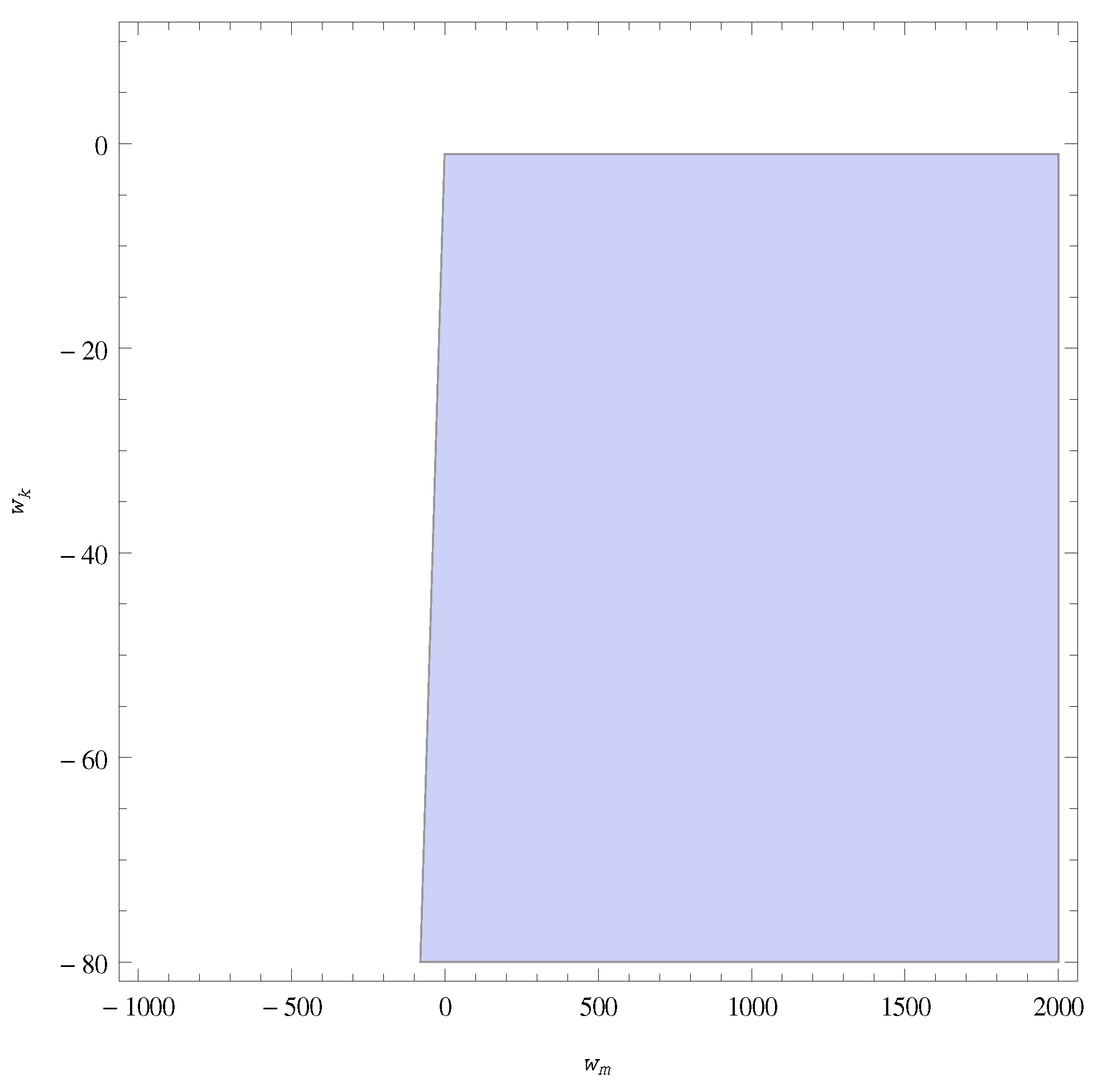
The second fixed point $(1,0,0,0)$ denotes a late time kinetic dominated universe with other dynamical variables $\tilde{y}$, $\tilde{z}$ and $\sigma$ becoming zero. In this case, eigenvalues are $(\frac{3(w_k+1)}{2},-1+\frac{3}{2}(1+w_k),\frac{3}{2}(-1+w_k+\frac{(1-w_k)(1+w_k)}{w_k}),3(w_k-w_m)).$ This is a stable fixed point for the region of parameter space shown in Figure 1.

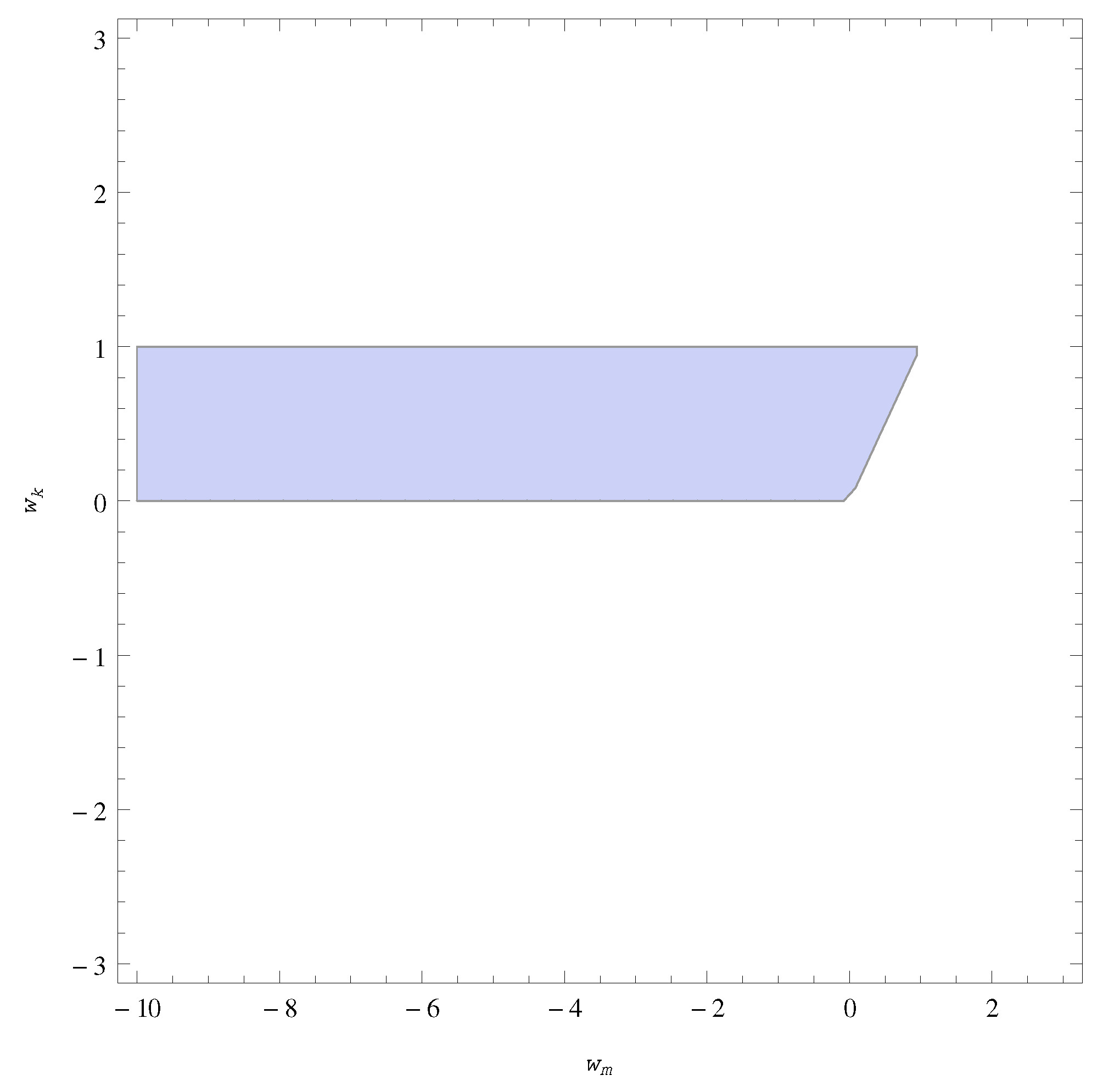
The next stable fixed point in this subsection is $(-1,0,0,0)$ with eigenvalue $(1+\frac{3}{2}(-1-w_k),\frac{3}{2}(-1-w_k),\frac{3(-1-w_k)(-1+w_k+\frac{(1-w_k)(1+w_k)}{w_k})}{2(1+w_k)},\frac{3}{2}(-1-w_k)-\frac{3}{2}(1+w_k)+3(1+w_m))$ shows again a late time kinetic dominated phase but with a negative value of Hubble parameter H signifying a contracting universe. This fixed point is found to be stable for the region of parameter space shown in Figure 2. The point $(-1,0,0,0)$ may not be important from a bouncing point of view, as we need the universe to transit to an expanding phase to be discussed in Section 4.

The remaining fixed points, in this section, being $(0,0,\sqrt{3}\frac{\sqrt{-w_k+w_m}}{\sqrt{1+3w_m}},0)$ for $w_m>w_k$ and $w_m>-\frac{1}{3}$, $(0,\frac{\sqrt{w_k-w_m}}{\sqrt{1+w_m}},0,0)$ with $w_k>w_m$ and $w_m>-1$, with eigen values

$(0,0,$$-\sqrt{\frac{3}{2}}\sqrt{w_k+3w_k^2-w_m-3w_k{w}_m},\sqrt{\frac{3}{2}}\sqrt{w_k+2w_k^2-w_m-3w_k{w}_m})$,

$(0,0,-\frac{3}{2}\sqrt{\frac{w_k+w_k^2-w_m-w_k{w}_m}{2}},$$\frac{3}{\sqrt{2}}\sqrt{w_k+w_k^2-w_m-w_k{w}_m})$ are also nonhyperbolic points. The stability of such fixed points goes beyond the linear stability analysis. All the fixed points and their stability conditions are noted in

Table 1. Stablity Analysis of fixed points for closed universe with $sign({\rho }_k)=+ve$.

Fixed Points $({\mathit{x}}_{\mathit{c}},{\mathit{y}}_{\mathit{c}},{\mathit{z}}_{\mathit{c}},{\mathit{\sigma }}_{\mathit{c}})$	Stability Conditions
$(0,0,0,0)$ for $w_k=w_m$	Ca not decide
$(1,0,0,0)$	Stable (see Figure 1)
$(-1,0,0,0)$	Stable (see Figure 2)
$(0,0,\sqrt{3}\frac{\sqrt{-w_k+w_m}}{\sqrt{1+3w_m}},0)$ with $w_m>w_k$ and $w_m>-\frac{1}{3}$	Ca not decide
$(0,\frac{\sqrt{w_k-w_m}}{\sqrt{1+w_m}},0,0)$ with $w_k>w_m$ and $w_m>-1$	Ca not decide

.

3.1.2. Case II, $sign({\rho }_k)=-ve$

In this section, we state the results of the stability analysis of our dynamical variables for the negative sign of kinetic energy density. The fixed points are found to be $(0,0,0,0)$, $(0,0,-\sqrt{3}\sqrt{\frac{w_k-w_m}{1+3w_m}},0)$ and $(0,\sqrt{\frac{-w_k+w_m}{1+w_m}},0,0)$ with eigen values $(0,0,0,0)$, $(0,0,$$-\sqrt{\frac{3}{2}}\sqrt{-w_k-3w_k^2+w_m+3w_k{w}_m}$, $\sqrt{\frac{3}{2}}\sqrt{-w_k-3w_k^2+w_m+3w_k{w}_m})$ and $(-3,0,0\frac{r{w}_k-w_k^2+w_m+w_k{w}_m}{\sqrt{2}},3\frac{\sqrt{w_k-w_k^2+w_m+w_k{w}_m}}{\sqrt{2}})$, respectively. All these fixed points are nonhyperbolic and tabulated in

Table 2. Stablity Analysis of fixed points for closed universe with $sign({\rho }_k)=-ve$.

Fixed Points $({\mathit{x}}_{\mathit{c}},{\mathit{y}}_{\mathit{c}},{\mathit{z}}_{\mathit{c}},{\mathit{\sigma }}_{\mathit{c}})$	Stability Conditions
$(0,0,0,0)$ for $w_k=w_m$	Ca not decide
$(0,0,-\sqrt{3}\sqrt{\frac{w_k-w_m}{1+3w_m}},0)$	Ca not decide
$(0,\sqrt{\frac{-w_k+w_m}{1+w_m}},0,0)$	Ca not decide

.

3.2. Open Universe

3.2.1. Case I, with $sign{\rho }_k=+ve$

In this case, we study the fixed points for all possible values of parameters in an FRW open universe. The fixed point $(0,0,0,0)$ is obtained for $w_k=w_m$ signifying all the dynamical variables $\tilde{x}$, $\tilde{y}$, $\tilde{z}$ and $\sigma$, going to zero at late times. It is a nonhyperbolic fixed point as the eigenvalue of $\mathbf{A}$ for this is $(0,0,0,0)$. Its stability cannot be decided from our first-order analysis of perturbations.

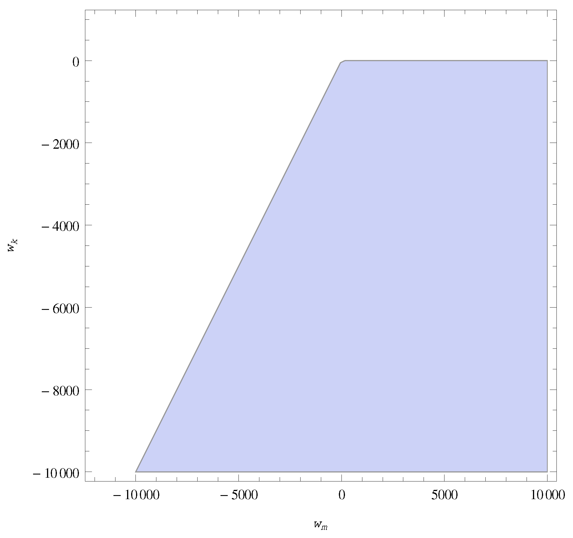
The second fixed point $(1,0,0,0)$ denotes a late time kinetic dominated universe with other dynamical variables $\tilde{y}$, $\tilde{z}$ and $\sigma$ becoming zero. In this case, eigenvalues are $(\frac{3(w_k+1)}{2},-1+\frac{3}{2}(1+w_k),\frac{3}{2}(-1+w_k+\frac{(1-w_k)(1+w_k)}{w_k}),3(w_k-w_m)).$ This is a stable fixed point for the region of parameter space shown in Figure 3.

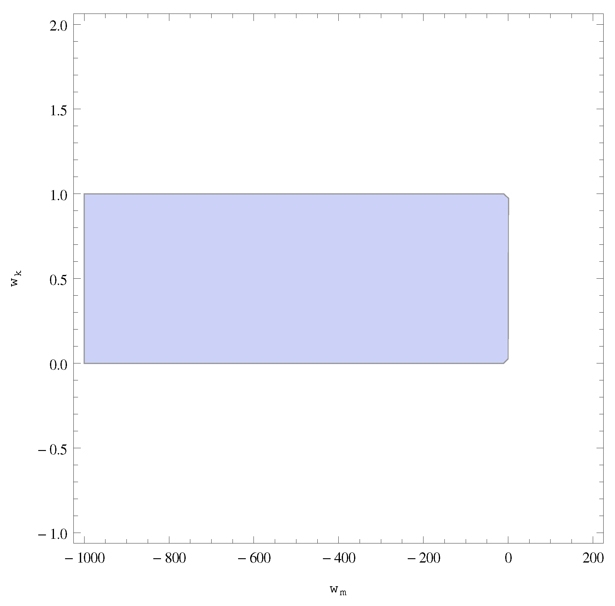
The next stable fixed point in this subsection is $(-1,0,0,0)$ with eigenvalue $(1+\frac{3}{2}(-1-w_k),\frac{3}{2}(-1-w_k),\frac{3(-1-w_k)(-1+w_k+\frac{(1-w_k)(1+w_k)}{w_k})}{2(1+w_k)},\frac{3}{2}(-1+w_k)-\frac{3}{2}(1+w_k)+3(1+w_m))$ shows again a late time kinetic dominated phase but with a negative value of Hubble parameter H signifying a contracting universe. This fixed point is found to be stable for the region of parameter space shown in Figure 4. The point $(-1,0,0,0)$ may not be important for the bouncing point of view, as again, we need the universe to transit to an expanding phase to be discussed in Section 4.

The remaining two fixed points being $(0,0,-\frac{\sqrt{3}\sqrt{w_k-w_m}}{\sqrt{1+3w_m}},0)$ with $w_k>w_m$ and $w_m>-\frac{1}{3}$ and $(0,\frac{\sqrt{w_k-w_m}}{\sqrt{1+w_m}},0,0)$ with $w_k>w_m$ and $w_m>-1$ with eigen values $(0,0,-\sqrt{\frac{3}{2}}\sqrt{w_k+3w_k^2-w_m-3w_k{w}_m},\sqrt{\frac{3}{2}}\sqrt{w_k+3w_k^2-w_m-3w_k{w}_m})$ and $(0,0,-\frac{3}{\sqrt{2}}\sqrt{w_k+w_k^2-w_m-w_k{w}_m},\frac{3}{\sqrt{2}}\sqrt{w_k+w_k^2-w_m-w_k{w}_m})$ are also nonhyperbolic points. The stability of such fixed points goes beyond the linear stability analysis. All the fixed points and their stability are noted in

Table 3. Stablity Analysis of fixed points for open universe with $sign({\rho }_k)=+ve$.

Fixed Points $({\mathit{x}}_{\mathit{c}},{\mathit{y}}_{\mathit{c}},{\mathit{z}}_{\mathit{c}},{\mathit{\sigma }}_{\mathit{c}})$	Stability Conditions
$(0,0,0,0)$ for $w_k=w_m$	Ca not decide
$(1,0,0,0)$	Stable (see Figure 3)
$(-1,0,0,0)$	Stable (see Figure 4)
$(0,0,-\frac{\sqrt{3}\sqrt{w_k-w_m}}{\sqrt{1+3w_m}},0)$ with $w_k>w_m$ and $w_m>-\frac{1}{3}$	Ca not decide
$(0,\frac{\sqrt{w_k-w_m}}{\sqrt{1+w_m}},0,0)$ with $w_k>w_m$ and $w_m>-1$	Ca not decide

.

3.2.2. Case II, $sign({\rho }_k)=-ve$

In this section, we state the results of the stability analysis of our dynamical variables for the negative sign of kinetic energy density. The fixed points are found to be $(0,0,0,0)$, $(0,0,$$-\sqrt{\frac{3(-w_k+w_m)}{1+3w_m}},0)$ with $w_m>w_k$ and $w_m>-\frac{1}{3}$, and $(0,\sqrt{\frac{-w_k+w_m}{1+w_m}},0,0)$ with $w_m>w_k$ and $w_m>-1$ with eigen values $(0,0,0,0)$, $(0,0,-\sqrt{\frac{3}{2}}\sqrt{-w_k-3w_k^2+w_m+3w_k{w}_m},$$\sqrt{\frac{3}{2}}\sqrt{-w_k-3w_k^2+w_m+3w_k{w}_m})$ and $(0,0,-\frac{3\sqrt{-w_k-w_k^2+w_m+w_k{w}_m}}{\sqrt{2}},\frac{3\sqrt{-w_k-w_k^2+w_m+w_k{w}_m}}{\sqrt{2}})$, respectively. All these fixed points are nonhyperbolic and tabulated in

Table 4. Stablity Analysis of fixed points for open universe with $sign({\rho }_k)=-ve$.

Fixed Points $({\mathit{x}}_{\mathit{c}},{\mathit{y}}_{\mathit{c}},{\mathit{z}}_{\mathit{c}},{\mathit{\sigma }}_{\mathit{c}})$	Stability Conditions
$(0,0,0,0)$ for $w_k=w_m$	Ca not decide
$(0,0,-\sqrt{\frac{3(-w_k+w_m)}{1+3w_m}},0)$ with $w_m>w_k$ and $w_m>-\frac{1}{3}$	Ca not decide
$(0,\sqrt{\frac{-w_k+w_m}{1+w_m}},0,0)$ with $w_m>w_k$ and $w_m>-1$	Ca not decide

.

4. Bouncing Scenario

Now we obtain the conditions for a nonsingular bounce to occur and also show the evolution of dynamical variables numerically. A nonsingular bounce is attained whenever the universe passes from a contracting phase to an expanding phase through a minimum value of the average scale factor $a(t),$ but not zero. Mathematically, it satisfies

$${(H)}_b\equiv \frac{1}{a_b(t)}{\left(\frac{\mathrm{d}a(t)}{\mathrm{d}t}\right)}_b=0,$$

(18)

where subscript b denotes the value of the variable at the bounce, and

$${\left(\frac{{\mathrm{d}}^{2}a(t)}{\mathrm{d}{t}^2}\right)}_b>0$$

(19)

for minimum to occur. This implies

$${\left(\frac{\mathrm{d}H}{\mathrm{d}t}\right)}_b={\left(\frac{\ddot{a}}{a}\right)}_b-{\left(\frac{\dot{a}}{a}\right)}_b^2>0$$

(20)

Now, writing the above conditions in terms of dynamical variables for bouncing, we get ${\tilde{x}}_b=0$ and ${\left(\frac{\mathrm{d}\tilde{x}}{\mathrm{d}\tilde{N}}\right)}_b>0$ which translate to the following equation

$${\left(\frac{\mathrm{d}\tilde{x}}{\mathrm{d}\tilde{N}}\right)}_b=-\frac{3}{2}\left[(w_k-w_m)(sign{\rho }_k)+(1+w_m)(-\tilde{y}|\tilde{y}|)+\frac{(1+3w_m)}{3}\tilde{z}\left|\tilde{z}\right|\right]>0$$

(21)

This implies

$${\left(\tilde{y}\widetilde{\left|y\right|}(1+w_m)-\tilde{z}\left|\tilde{z}\right|(1+3w_m)\right)}_b>1\times sign({\rho }_k)(w_k-w_m)$$

(22)

At the bounce, we then obtain the constraint equation among dynamical variables as

$${\left({\tilde{x}}^2-\tilde{y}\widetilde{\left|y\right|}+\tilde{z}\left|\tilde{z}\right|-{\tilde{\Omega }}_m\right)}_b=-\tilde{y}\widetilde{\left|y\right|}+\tilde{z}\left|\tilde{z}\right|-{\tilde{\Omega }}_m=1\times sign({\rho }_k)$$

(23)

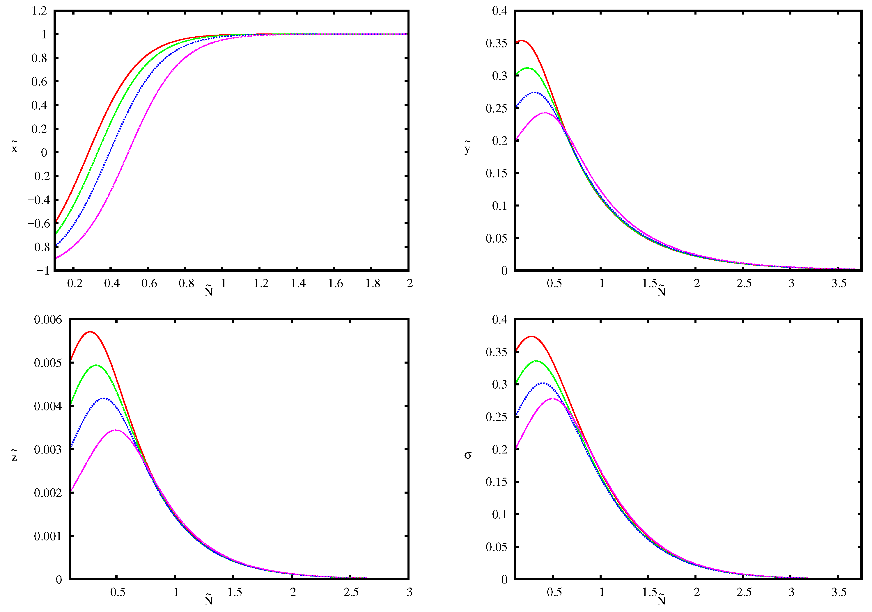
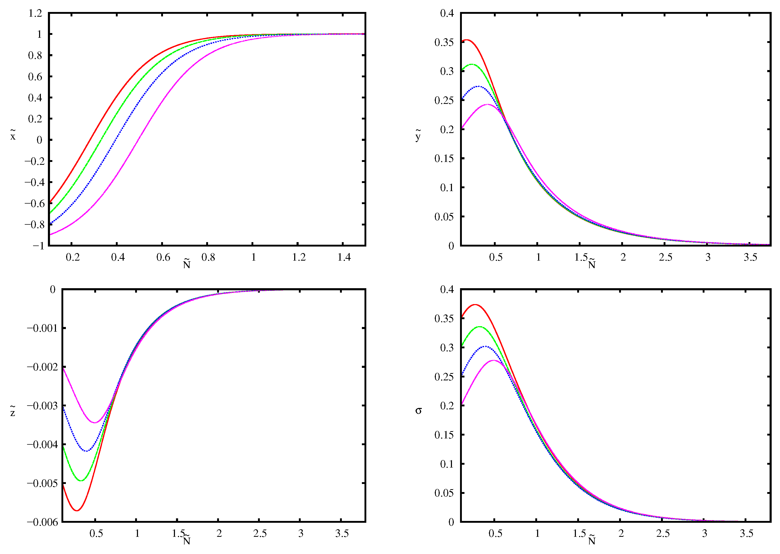
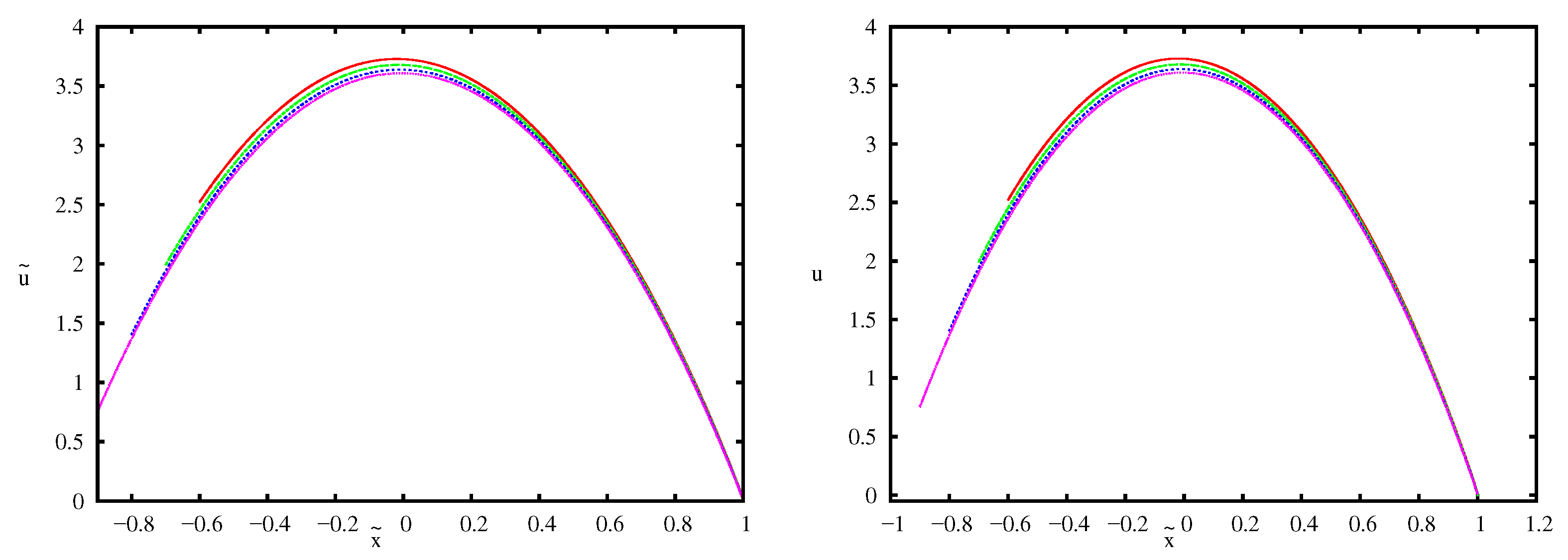
Now, for different negative initial conditions of $\tilde{x}$ (contracting phase), Figure 5 (top left) and Figure 6 (top left) for the closed and open universe, respectively, show its transition to positive values (expanding phase) crossing zero (bounce). The bouncing is guaranteed by the positivity of the slope of $\tilde{x}$ as shown in Figure 7 (left plot for closed and right plot for open). Thus, the top left of Figure 5, Figure 6 and Figure 7, together, do indeed represent a stable bouncing scenario in an FRW closed and open universe. This is obtained by setting the values of the equation of state parameters $w_k=-2$$(\eta =1/4),$$w_m=1/3$ and $sign({\rho }_k)=+ve$ and $sign(y)=+ve$. The evolution of other dynamical variables can be seen in Figure 5 and Figure 6, which show their asymptotic evolution to the respective fixed points for the same choice of parameters.

It can be seen that the fixed point $({\tilde{x}}_c,{\tilde{y}}_c,{\tilde{z}}_c,{\sigma }_c)=(1,0,0,0)$ does give rise to a stable bouncing universe as it satisfies Equations (22) and (23) for open ($sign(\tilde{z})$ = −ve) and closed ($sign(\tilde{z})$ = +ve) universe. From this analysis, we conclude that finally after the bounce our universe at late times is driven by kinetic energy density in both cases. The other fixed point $(-1,0,0,0)$, though stable, can not give rise to a bouncing scenario as it ends up with a negative value of the Hubble parameter, H, signifying a late time contracting phase.

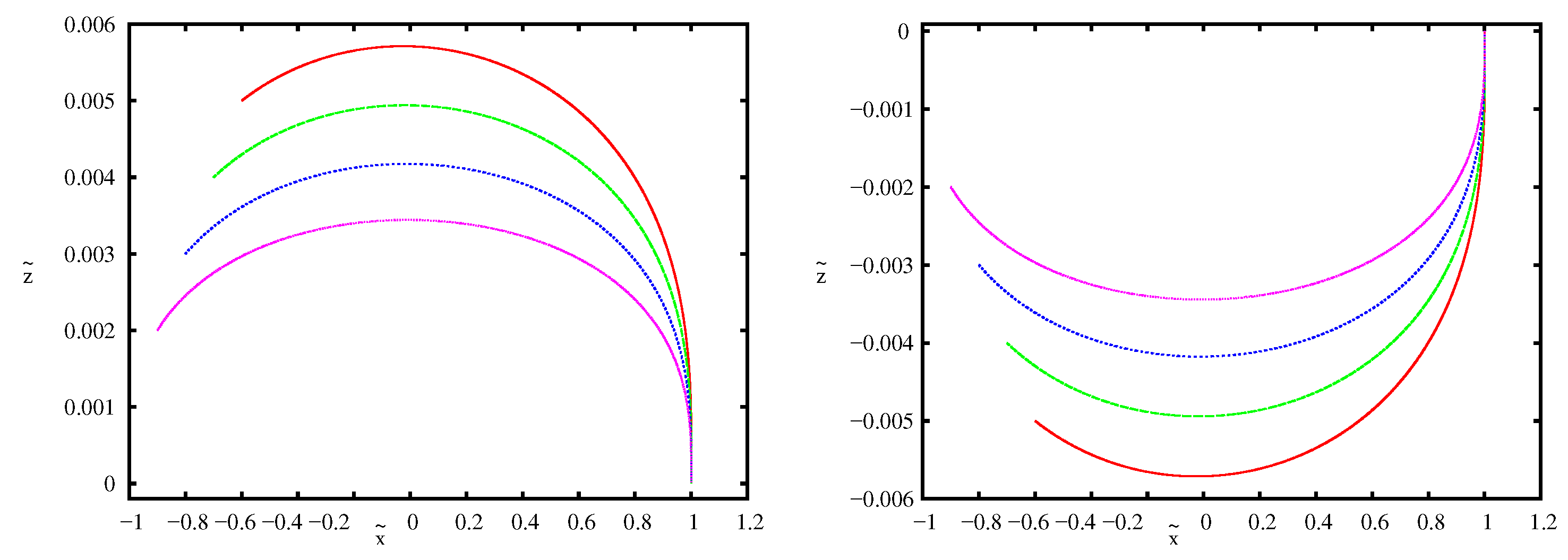
Furthermore, we show the behavior of the curvature parameter, $\tilde{z},$ in this nonsingular bouncing setup. The curvature parameter increases initially in the contracting phase reaching an extremum at the bounce and then decreases to zero in the expanding phase as shown in Figure 8 for both open and closed universe. Thus, the curvature parameter remains finite at the bounce as expected in a nonsingular bouncing scenario and at late time universe becomes flat irrespective of whether we start initially with closed or open. This may be useful for building realistic models.

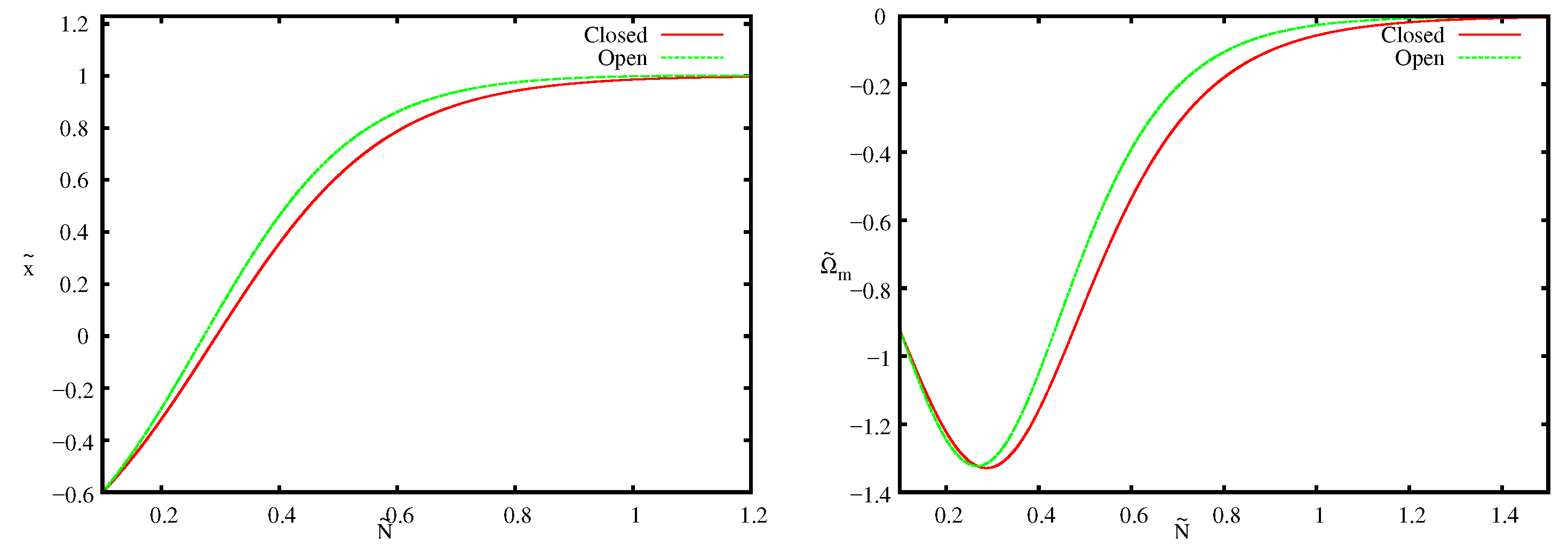
The comparison between bouncing solutions for open and closed is done in Figure 9. It has been found that bouncing occurs earlier in the case of an open than in a closed universe as shown in the left-hand side of Figure 9 for the same set of initial conditions and parameters. Furthermore, it is noted that, though the solutions differ appreciably near the bounce, they approach the same value at a late time owing to the zero value of the curvature parameter. The nonsingular bounce happens only for negative values of ${\tilde{\Omega }}_m$ with our choice of parameters as shown in Figure 9 (right) for both open and closed universe.

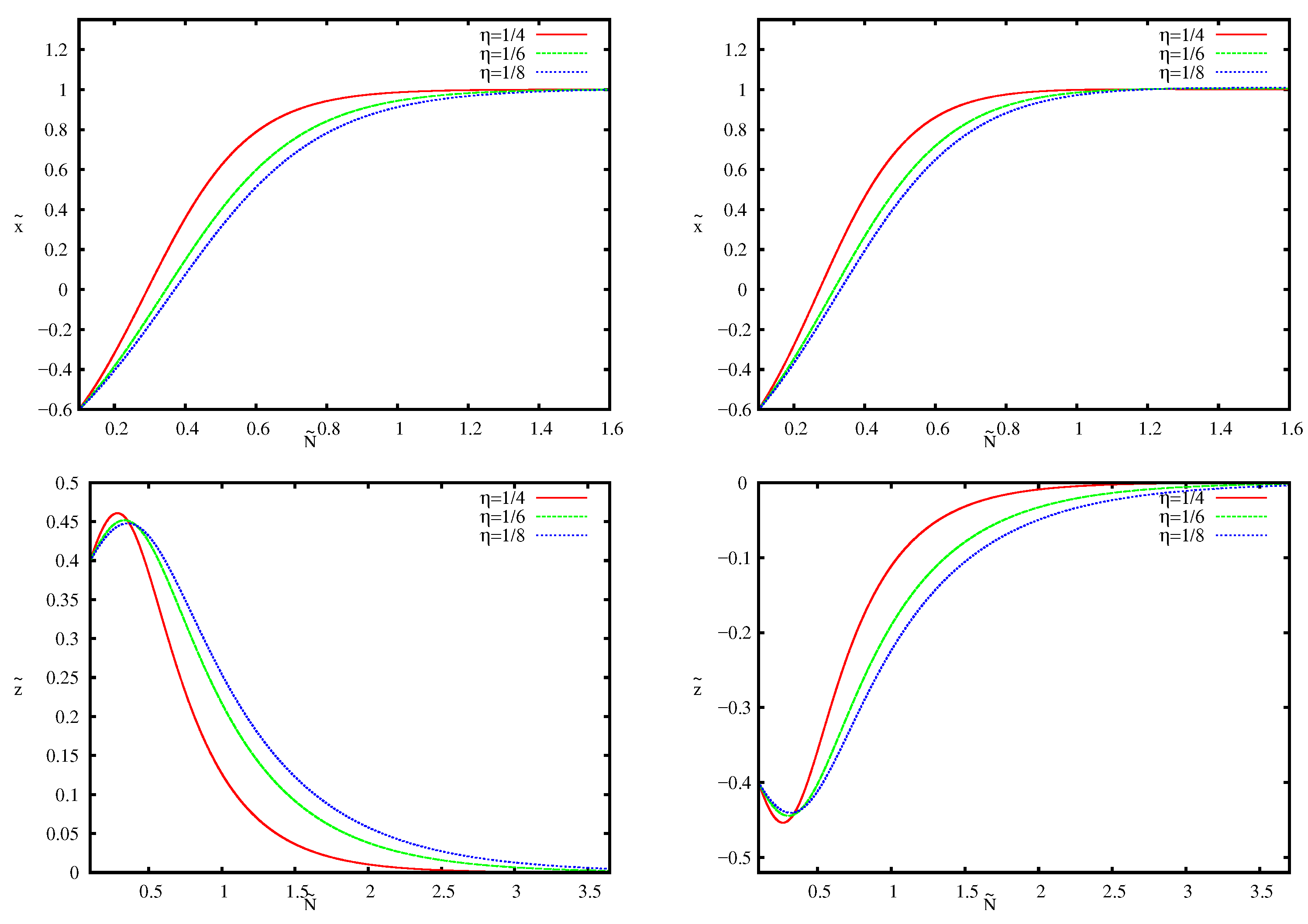
Finally, we show the effect of different values of $\eta$ on the behavior of bouncing solutions in Figure 10 for both closed and open universes. All the plots are generated for the same set of initial conditions and the same set of parameters $w_m=1/3$, $sign({\rho }_k)=+ve$ but with three different values of parameters $\eta =1/4$, $1/6$ and $1/8$. It has been observed that the value of $\eta$ has a direct impact on the occurrence of the bouncing point. Indeed, the position of the bouncing point is delayed as we decrease the value of $\eta$ for both closed and open universe as shown in Figure 10 (top left and top right). The bottom left and bottom right of Figure 10 indicate the effect of $\eta$ on the curvature parameter for both closed and open cases, respectively. It has been found that the magnitude of the maximum value of $\tilde{z},$ at the bounce, decreases as we decrease the value of $\eta .$

5. Conclusions

A cosmological scenario with a noncanonical scalar field and matter is explored in this work. Using dynamical equations for a set of dimensionless dynamical variables, we find all the fixed points for the two cases with positive and negative kinetic energy density terms in FRW closed and the open universe. Allowed regions of parameter spaces for the stability of fixed points are shown for both cases. The necessary and sufficient conditions for a nonsingular bounce are obtained in terms of the dynamical variables. Thus, stable bouncing solutions are obtained by satisfying nonsingular bouncing conditions and stability criteria. This is achieved for the negative energy density of matter, ${\tilde{\Omega }}_m,$ with the equation of state parameter $w_m=1/3$ in both closed and open universe. In addition to this, the finitude of curvature parameter at the bounce is obtained as expected in a nonsingular bouncing scenario and the universe becomes flat at a late time irrespective of whether we start with a closed or open one. Finally, the effect of the parameter $\eta$ on the behavior of the bouncing solution is noted. It is seen that the point of occurrence of bounce is delayed as we decrease the value of $\eta$ and the magnitude of the value of curvature parameter at the bounce decreases with $\eta$ for both open and closed universe.

We restrict our analysis to a positive sign of potential. It is straightforward to extend our analysis for a negative potential by changing the parameter $sign(y)$ to $-1$.

As mentioned above this work is in the classical regime. Furthermore, it is obvious that there are two ways to solve the initial singularity: Either by invoking modification in the matter sector or by modifying the gravity sector which includes modified theories of gravity. However, none of these modifications deals with the physics at the Planck region. The popularly known inflationary paradigm which predicts the formation of the structure still treats spacetime to be classical and obviously this can not be correct at the high curvature limit.

This is interesting and a matter of paramount importance to include quantum effects. In the next series of works, we propose to formulate the present model in the framework of loop quantum cosmology. The loop quantum cosmology in the case of a minimally coupled scalar field is well studied. Our future work would involve studying the effective dynamics due to non-trivial Lagrangian like the present case. This would be followed by a detailed dynamical system analysis of the phase space.

References

- Finelli, F.; Brandenberger, R. On the generation of a scale-invariant spectrum of adiabatic fluctuations in cosmological models with a contracting phase. Phys. Rev. D 2002, 65, 103522. [Google Scholar] [CrossRef]
- Khoury, J.; Ovrut, B.A.; Steinhardt, P.J.; Turok, N. The ekpyrotic universe: Colliding branes and the origin of the hot big bang. Phys. Rev. D 2001, 64, 123522. [Google Scholar] [CrossRef]
- Khoury, J.; Ovrut, B.A.; Seiberg, N.; Steinhardt, P.J.; Turok, N. From big crunch to big bang. Phys. Rev. D 2002, 65, 086007. [Google Scholar] [CrossRef]
- Brandenberger, R.H. Alternatives to Cosmological Inflation. arXiv 2009, arXiv:0902.4731. [Google Scholar] [CrossRef]
- Brandenberger, R.H. Cosmology of the Very Early Universe. AIP Conf. Proc. 2010, 1268, 3–70. [Google Scholar]
- Brandenberger, R.H. Introduction to Early Universe Cosmology. arXiv 2010, arXiv:1103.2271. [Google Scholar]
- Brandenberger, R.H. The Matter Bounce Alternative to Inflationary Cosmology. arXiv 2012, arXiv:1206.4196. [Google Scholar]
- Lehners, J.-L. Ekpyrotic and Cyclic Cosmology. Phys. Rept. 2008, 465, 223. [Google Scholar] [CrossRef]
- Panda, S.; Sharma, M. Anisotropic bouncing scenario in F(X)−V(ϕ) model. Astrophys. Space Sci. 2016, 361, 87. [Google Scholar] [CrossRef]
- Mukhanov, V.F.; Vikman, A. Enhancing the tensor-to-scalar ratio in simple inflation. JCAP 2006, 0602, 4. [Google Scholar] [CrossRef]
- Panotopoulos, G. Detectable primordial non-gaussianities and gravitational waves in k-inflation. Phys. Rev. D 2007, 76, 127302. [Google Scholar] [CrossRef]
- Unnikrishnan, S.; Sahni, V.; Toporensky, A. Refining inflation using non-canonical scalars. JCAP 2012, 1208, 18. [Google Scholar] [CrossRef]
- Chiba, T.; Okabe, T.; Yamaguchi, M. Kinetically driven quintessence. Phys. Rev. D 2000, 62, 023511. [Google Scholar] [CrossRef]
- Copeland, E.J.; Sami, M.; Tsujikawa, S. Dynamics of dark energy. Int. J. Mod. Phys. D 2006, 15, 1753. [Google Scholar] [CrossRef]
- Bertacca, D.; Bartolo, N.; Matarrese, S. Unified Dark Matter Scalar Field Models. Adv. Astron. 2010, 2010, 904379. [Google Scholar] [CrossRef]
- Bose, N.; Majumdar, A.S. A k-essence Model Of Inflation, Dark Matter and Dark Energy. Phys. Rev. D 2009, 79, 103517. [Google Scholar] [CrossRef]
- Bose, N.; Majumdar, A.S. Unified Model of k-Inflation, Dark Matter and Dark Energy. Phys. Rev. D 2009, 80, 103508. [Google Scholar] [CrossRef]
- De-Santiago, J.; Cervantes-Cota, J.L. Generalizing a Unified Model of Dark Matter, Dark Energy, and Inflation with Non Canonical Kinetic Term. Phys. Rev. D 2011, 83, 063502. [Google Scholar] [CrossRef]
- Copeland, E.J.; Liddle, A.R.; Wands, D. Exponential potentials and cosmological scaling solutions. Phys. Rev. D 1998, 57, 4686. [Google Scholar] [CrossRef]
- De-Santiago, J.; Cervantes-Cota, J.L.; Wands, D. Cosmological phase space analysis of the F (X) - V (phi) scalar field and bouncing solutions. Phys. Rev. D 2013, 87, 023502. [Google Scholar] [CrossRef]
Figure 1.
Allowed region of parameter space for the fixed point in closed universe.
Figure 2.
Figure 3.
Allowed region of parameter space for the fixed point in open universe.
Figure 4.
Figure 5.
Evolution of the dynamical variables (top left), (top right), (bottom left) and (bottom right) for the fixed point with the values of parameters , , and for different initial conditions.
Figure 6.
Figure 7.
vs. for closed (left) and for open (right) with , and .
Figure 8.
Figure 9.
Comparision between closed and open for vs. (left) and vs. (right) with , and .
Figure 10.
Evolution for closed (top left) and open (top right); for closed (bottom left) and open (bottom right) with values and , and .