Consistent Estimation of Generalized Linear Models with High Dimensional Predictors via Stepwise Regression

Abstract

Predictive models play a central role in decision making. Penalized regression approaches, such as least absolute shrinkage and selection operator (LASSO), have been widely used to construct predictive models and explain the impacts of the selected predictors, but the estimates are typically biased. Moreover, when data are ultrahigh-dimensional, penalized regression is usable only after applying variable screening methods to downsize variables. We propose a stepwise procedure for fitting generalized linear models with ultrahigh dimensional predictors. Our procedure can provide a final model; control both false negatives and false positives; and yield consistent estimates, which are useful to gauge the actual effect size of risk factors. Simulations and applications to two clinical studies verify the utility of the method.

1. Introduction

In the era of precision medicine, constructing interpretable and accurate predictive models, based on patients’ demographic characteristics, clinical conditions and molecular biomarkers, has been crucial for disease prevention, early diagnosis and targeted therapy [1]. When the number of predictors is moderate, penalized regression approaches such as least absolute shrinkage and selection operator (LASSO) by [2] have been used to construct predictive models and explain the impacts of the selected predictors. However, in ultrahigh dimensional settings where p is in the exponential order of n, penalized methods may incur computational challenges [3], may not reach globally optimal solutions and often generate biased estimates [4]. Sure independence screening (SIS) proposed by [5] has emerged as a powerful tool for modeling ultrahigh dimensional data. However, the method relies on a partial faithfulness assumption, which stipulates that jointly important variables must be marginally important, an assumption that may not be always realistic. To relieve this condition, some iterative procedures, such as ISIS [5], have been adopted to repeatedly screen variables based on the residuals from the previous iterations, but with heavy computation and unclear theoretical properties. Conditional screening approaches [see, e.g., [6]] have, to some extent, addressed the challenge. However, screening methods do not directly generate a final model, and post-screening regularization methods, such as LASSO, are recommended by [5] to produce a final model.

For generating a final predictive model in ultrahigh dimensional settings, recent years have seen a surging interest of performing forward regression, an old technique for model selection; see [7,8,9], among many others. Under some regularity conditions and with some proper stopping criteria, forward regression can achieve screening consistency and sequentially select variables according to metrics such as AIC, BIC or $R^2$. Closely related to forward selection also, is least angle regression (LARS) [10], a widely used model selection algorithm for high-dimensional models. In the generalized linear model setting [11,12], proposed differential geometrical LARS (dgLARS) based on a differential geometrical extension of LARS.

However, these methods have drawbacks. First, once a variable is identified by the forward selection, it is not removable from the list of selected variables. Hence, false positives are unavoidable without a systematic elimination procedure. Second, most of the existing works focus on variable selection and are silent with respect to estimation accuracy.

To address the first issue, some works have been proposed to add backward elimination steps once forward selection is accomplished, as backward elimination may further eliminate false positives from the variables selected by forward selection. For example, ref. [13,14] proposed a stepwise selection for linear regression models in high-dimensional settings and proved model selection consistency. However, it is unclear whether the results hold for high-dimensional generalized linear models (GLMs); Ref. [15] proposed a similar stepwise algorithm in high-dimensional GLM settings, but with no theoretical properties on model selection. Moreover, none of the relevant works have touched upon the accuracy of estimation.

We extend a stepwise regression method to accommodate GLMs with high-dimensional predictors. Our method embraces both model selection and estimation. It starts with an empty model or pre-specified predictors, scans all features and sequentially selects features, and conducts backward elimination once forward selection is completed. Our proposal controls both false negatives and false positives in high dimensional settings: the forward selection steps recruit variables in an inclusive way by allowing some false positives for the sake of avoiding false negatives, while the backward selection steps eliminate the potential false positives from the recruited variables. We use different stopping criteria in the forward and backward selection steps, to control the numbers of false positives and false negatives. Moreover, we prove that, under a sparsity assumption of the true model, the proposed approach can discover all of the relevant predictors within a finite number of steps, and the estimated coefficients are consistent, a property still unknown to the literature. Finally, our GLM framework enables our work to accommodate a wide range of data types, such as binary, categorical and count data.

To recap, our proposed method distinguishes from the existing stepwise approaches in high dimensional settings. For example, it improves  [13,14] by extending the work to a more broad GLM setting and  [15] by establishing the theoretical properties.

Compared with the other variable selection and screening works, our method produces a final model in ultrahigh dimensional settings, without applying a pre-screening step which may produce unintended false negatives. Under some regularity conditions, the method identifies or includes the true model with probability going to 1. Moreover, unlike the penalized approaches such as LASSO, the coefficients estimated by our stepwise selection procedure in the final model will be consistent, which are useful for gauging the real effect sizes of risk factors.

2. Method

Let $({\mathbf{X}}_i,Y_i),i=1,\dots ,n,$ denote n independently and identically distributed (i.i.d.) copies of $(\mathbf{X},Y)$. Here, $\mathbf{X}={(1,X_1,\dots ,X_p)}^{\mathrm{T}}$ is a $(p+1)$-dimensional predictor vector with $X_0=1$ corresponding to the intercept term, and Y is an outcome. Suppose that the conditional density of Y, given $\mathbf{X}$, belongs to a linear exponential family:

$$\begin{array}{c}\hfill \pi (Y\mid \mathbf{X})=exp\{Y{\mathbf{X}}^{\mathrm{T}}\mathit{\beta }-b\left({\mathbf{X}}^{\mathrm{T}}\mathit{\beta }\right)+\mathcal{A}\left(Y\right)\},\end{array}$$

(1)

where $\mathit{\beta }={({\beta }_0,{\beta }_1,\dots ,{\beta }_p)}^{\mathrm{T}}$ is the vector of coefficients; ${\beta }_0$ is the intercept; and $\mathcal{A}\left(·\right)$ and $b\left(·\right)$ are known functions. Model (1), with a canonical link function and a unit dispersion parameter, belongs to a larger exponential family [16]. Further, $b\left(·\right)$ is assumed twice continuously differentiable with a non-negative second derivative $b^{\prime \prime }\left(·\right)$. We use $\mu \left(·\right)$ and $\sigma \left(·\right)$ to denote $b^{\prime }\left(·\right)$ and $b^{\prime \prime }\left(·\right)$, i.e., the mean and variance functions, respectively. For example, $b\left(\theta \right)=log(1+exp(\theta \left)\right)$ in a logistic distribution and $b\left(\theta \right)=exp\left(\theta \right)$ in a Poisson distribution.

Let $L(u,v)=uv-b\left(u\right)$ and ${\mathbb{E}}_n\left\{f\left(\xi \right)\right\}=n^{-1}{\sum }_{i=1}^{n}f\left({\xi }_i\right)$ denote the mean of ${\left\{f\left({\xi }_i\right)\right\}}_{i=1}^n$ for a sequence of i.i.d. random variables ${\xi }_i$$(i=1,\dots ,n)$ and a non-random function $f\left(·\right)$. Based on the i.i.d. observations, the log-likelihood function is

$$\begin{array}{c}\hfill \ell \left(\mathit{\beta }\right)=n^{-1}\sum _{i=1}^{n}L({\mathbf{X}}_i^{\mathrm{T}}\mathit{\beta },Y_i)={\mathbb{E}}_n\left\{L({\mathbf{X}}^{\mathrm{T}}\mathit{\beta },Y)\right\}.\end{array}$$

(2)

We use ${\mathit{\beta }}_{*}={({\beta }_{*0},{\beta }_{*1},\dots ,{\beta }_{*p})}^{\mathrm{T}}$ to denote the true values of $\mathit{\beta }$. Then the true model is $\mathcal{M}=\{j:{\beta }_{*j}\ne 0,j\ge 1\}\cup \left\{0\right\}$, which consists of the intercept and all variables with nonzero effects. Overarching goals of ultra-high dimensional data analysis are to identify $\mathcal{M}$ and estimate ${\beta }_{*j}$ for $j\in \mathcal{M}$. While most of the relevant literature [8,9] is on estimating $\mathcal{M}$, this work is to accomplish both identification of $\mathcal{M}$ and estimation of ${\beta }_{*j}$.

When p is in the exponential order of n, we aim to generate a predictive model that contains the true model with high probability, and provide consistent estimates of regression coefficients. We further introduce the following notation. For a generic index set $S\subset \{0,1,\dots ,p\}$ and a $(p+1)$-dimensional vector $\mathbf{A}$, we use $S^c$ to denote the complement of a set S and ${\mathbf{A}}_S=\{A_j:j\in S\}$ to denote the subvector of $\mathbf{A}$ corresponding to S. For instance, if $S=\{2,3,4\}$, then ${\mathbf{X}}_{iS}={(X_{i2},X_{i3},X_{i4})}^{\mathrm{T}}$. Moreover, denote by ${\ell }_S\left({\mathit{\beta }}_S\right)={\mathbb{E}}_n\left\{L({\mathbf{X}}_S^{\mathrm{T}}{\mathit{\beta }}_S,Y)\right\}$ the log-likelihood of the regression model of Y on ${\mathbf{X}}_S$ and denote by ${\widehat{\mathit{\beta }}}_S$ the maximizer of ${\ell }_S\left({\mathit{\beta }}_S\right)$. Under model (1), we elaborate on the idea of stepwise (details in the supplementary materials) selection, consisting of the forward and backward stages.

Forward stage: We start with $F_0$, a set of variables that need to be included according to some a priori knowledge, such as clinically important factors and conditions. If no such information is available, $F_0$ is set to be $\left\{0\right\}$, corresponding to a null model. We sequentially add covariates as follows:

$$F_0\subset F_1\subset F_2\subset \cdots \subset F_k,$$

where $F_k\subset \{0,1,\dots ,p\}$ is the index set of the selected covariates upon completion of the kth step, with $k\ge 0$. At the $(k+1)$th step, we append new variables to $F_k$ one at a time and refit GLMs: for every $j\in F_k^c$, we let $F_{k,j}=F_k\cup \left\{j\right\}$, obtain ${\widehat{\mathit{\beta }}}_{F_{k,j}}$ by maximizing ${\ell }_{F_{k,j}}\left({\mathit{\beta }}_{F_{k,j}}\right)$, and compute the increment of log-likelihood,

$${\ell }_{F_{k,j}}\left({\widehat{\mathit{\beta }}}_{F_{k,j}}\right)-{\ell }_{F_k}\left({\widehat{\mathit{\beta }}}_{F_k}\right).$$

Then the index of a new candidate variable is determined to be

$$j_{k+1}=\underset{j\in F_k^c}{arg\; max}{\ell }_{F_{k,j}}\left({\widehat{\mathit{\beta }}}_{F_{k,j}}\right)-{\ell }_{F_k}\left({\widehat{\mathit{\beta }}}_{F_k}\right).$$

Additionally, we update $F_{k+1}=F_k\cup \left\{j_{k+1}\right\}.$ We then need to decide whether to stop at the kth step or move on to the $(k+1)$th step with $F_{k+1}$. To do so, we use the following EBIC criterion:

$$EBIC\left(F_{k+1}\right)=-2{\ell }_{F_{k+1}}\left({\widehat{\mathit{\beta }}}_{F_{k+1}}\right)+\left|F_{k+1}\right|n^{-1}(logn+2{\eta }_{1}logp),$$

(3)

where the second term is motivated by [17] and $\left|F\right|$ denotes the cardinality of a set F.

The forward selection stops if $EBIC\left(F_{k+1}\right)>EBIC\left(F_k\right)$. We denote the stopping step by $k^{*}$ and the set of variables selected so far by $F_{k^{*}}$.

Backward stage: Upon the completion of forward stage, backward elimination, starting with $B_0=F_{k^{*}}$, sequentially drops covariates as follows:

$$B_0\supset B_1\supset B_2\supset \cdots \supset B_k,$$

where $B_k$ is the index set of the remaining covariates upon the completion of the kth step of the backward stage, with $k\ge 0$. At the $(k+1)$th backward step and for every $j\in B_k$, we let $B_{k/j}=B_k\backslash \left\{j\right\}$, obtain ${\widehat{\mathit{\beta }}}_{B_{k/j}}$ by maximizing $\ell \left({\mathit{\beta }}_{B_{k/j}}\right)$, and calculating the difference of the log-likelihoods between these two nested models:

$${\ell }_{B_k}\left({\widehat{\mathit{\beta }}}_{B_k}\right)-{\ell }_{B_{k/j}}\left({\widehat{\mathit{\beta }}}_{B_{k/j}}\right).$$

The variable that can be removed from the current set of variables is indexed by

$$j_{k+1}=\underset{j\in B_k}{arg\; min}{\ell }_{B_k}\left({\widehat{\mathit{\beta }}}_{B_k}\right)-{\ell }_{B_{k/j}}\left({\widehat{\mathit{\beta }}}_{B_{k/j}}\right).$$

Let $B_{k+1}=B_k\backslash \left\{j_{k+1}\right\}.$ We determine whether to stop at the kth step or move on to the ($k+1$)th step of the backward stage according to the following BIC criterion:

$$BIC\left(B_{k+1}\right)=-2{\ell }_{B_{k+1}}\left({\widehat{\mathit{\beta }}}_{B_{k+1}}\right)+{\eta }_2{n}^{-1}\left|B_{k+1}\right|logn.$$

(4)

If $BIC\left(B_{k+1}\right)>BIC\left(B_k\right)$, we end the backward stage at the kth step. Let $k^{**}$ denote the stopping step and we declare the selected model $B_{k^{**}}$ to be the final model. Thus, $\widehat{\mathcal{M}}=B_{k^{**}}$ is the estimate of $\mathcal{M}$. As the backward stage starts with the $k^{*}$ variables selected by forward selection, $k^{**}$ cannot exceed $k^{*}$.

A strength of our algorithm, termed STEPWISE hereafter, is the added flexibility with ${\eta }_1$ and ${\eta }_2$ in the stopping criteria for controlling the false negatives and positives. For example, a smaller value of ${\eta }_1$ close to zero in the forward selection step will likely include more variables, and thus incur more false positives and less false negatives, whereas a larger value of ${\eta }_1$ will recruit too few variables and cause too many false negatives. Similarly, in the backward selection step, a large ${\eta }_2$ would eliminate more variables and therefore further reduce more false positives, and vice versa for a small ${\eta }_2$. While finding optimal ${\eta }_1$ and ${\eta }_2$ is not trivial, our numerical experiences suggest a small ${\eta }_1$ and a large ${\eta }_2$ may well balance the false negatives and positives. When ${\eta }_2=0$, no variables can be dropped after forward selection; hence, our proposal includes forward selection as a special case.

Moreover, [8] proposed a sequentially conditioning approach based on offset terms that absorb the prior information. However, our numerical experiments indicate that the offset approach may be suboptimal compared to our full stepwise optimization approach, which will be demonstrated in the simulation studies.

3. Theoretical Properties

With a column vector $\mathbf{v}$, let ${\parallel \mathbf{v}\parallel }_q$ denote the $L_q$-norm for any $q\ge 1$. For simplicity, we denote the $L_2$-norm of $\mathbf{v}$ by $\parallel \mathbf{v}\parallel$, and denote $\mathbf{v}{\mathbf{v}}^{\mathrm{T}}$ by ${\mathbf{v}}^{\otimes 2}$. We use $C_1,C_2,\dots ,$ to denote some generic constants that do not depend on n and may change from line to line. The following regularity conditions are set.

• There exist a positive integer q satisfying $\left|\mathcal{M}\right|\le q$ and $qlogp=o\left(n^{1/3}\right)$ and a constant $K>0$ such that ${sup}_{\left|S\right|\le q}{\parallel {\mathit{\beta }}_S^{*}\parallel }_1\le K$, where ${\mathit{\beta }}_S^{*}={arg\; max}_{{\mathit{\beta }}_S}E\left[{\ell }_S\left({\mathit{\beta }}_S\right)\right]$ is termed the least false value of model S.
• ${\parallel \mathbf{X}\parallel }_{\infty }\le K$. In addition, $E\left(X_j\right)=0$ and $E\left(X_j^2\right)=1$ for $j\ge 1$.
• Let ${ϵ}_i=Y_i-\mu \left({\mathit{\beta }}_{*}^{\mathrm{T}}{\mathbf{X}}_i\right)$. There exists a positive constant M such that the Cramer condition holds, i.e., $E\left[{\left|{ϵ}_i\right|}^m\right]\le m!M^m$ for all $m\ge 1$.
• $\left|\sigma \right(a)-\sigma (b\left)\right|\le K|a-b|$ and ${\sigma }_{min}:={inf}_{\left|t\right|\le K^3}\left|b^{\prime \prime }\left(t\right)\right|$ is bounded below.
• There exist two positive constants, ${\kappa }_{min}$ and ${\kappa }_{max}$ such that $0<{\kappa }_{min}<\Lambda \left(E\left({\mathbf{X}}_S^{\otimes 2}\right)\right)<{\kappa }_{max}<\infty$, uniformly in $S\subset \{0,1,\dots ,p\}$ satisfying $\left|S\right|\le q$, where $\Lambda \left(\mathbf{A}\right)$ is the collection of all eigenvalues of a square matrix $\mathbf{A}$.
• ${min}_{S:\mathcal{M}⊈S,\left|S\right|\le q}{D}_S>C{n}^{-\alpha }$ for some constants $C>0$ and $\alpha >0$ that satisfies $q{n}^{-1+4\alpha }logp\to 0$, where $D_S={max}_{j\in {\mathcal{S}}^c\cap \mathcal{M}}\left|E\left[\left(\mu \left({\mathit{\beta }}_{*}^{\mathrm{T}}\mathbf{X}\right)-\mu \left({\mathit{\beta }}_S^{*\mathrm{T}}{\mathbf{X}}_S\right)\right)X_j\right]\right|$.

Condition (1), as assumed in  [8,18], is an alternative to the Lipschitz assumption [5,19]. The bound of the model size allowed in the selection procedure or q is often required in model-based screening methods see, e.g., [8,20,21,22]. The bound should be large enough so that the correct model can be included, but not too large; otherwise, excessive noise variables would be included, leading to unstable and inconsistent estimates. Indeed, Conditions (1) and (6) reveal that the range of q depends on the true model size $\left|\mathcal{M}\right|$, the minimum signal strength, $n^{-\alpha }$ and the total number of covariates, p. The upper bound of q is $o((n^{1-4\alpha }/logp)\wedge (n^{1/3}/logp))$, ensuring the consistency of EBIC [17]. Condition (1) also implies that the parameter space under consideration can be restricted to $\mathbb{B}:=\{\mathit{\beta }\in {\mathbb{R}}^{p+1}:\parallel \mathit{\beta }{\parallel }_1\le K^2\}$, for any model S with $\left|S\right|\le q$. Condition (2), as assumed in  [23,24], reflects that data are often standardized at the pre-processing stage. Condition (3) ensures that Y has a light tail, and is satisfied by Gaussian and discrete data, such as binary and count data [25]. Condition (4) is satisfied by common GLM models, such as Gaussian, binomial, Poisson and gamma distributions. Condition (5) represents the sparse Riesz condition [26] and Condition (6) is a strong "irrepresentable" condition, suggesting that $\mathcal{M}$ cannot be represented by a set of variables that does not include the true model. It further implies that adding a signal variable to a mis-specified model will increase the log-likelihood by a certain lower bound [8]. The signal rate is comparable to the conditions required by the other sequential methods, see, e.g., [7,22].

Theorem 1 develops a lower bound of the increment of the log-likelihood if the true model $\mathcal{M}$ is not yet included in a selected model S.

Theorem 1.

Suppose Conditions (1)–(6) hold. There exists some constant $C_1$ such that with probability at least 1–6$exp(-6qlogp)$,

$$\begin{array}{c}\hfill \underset{S:\mathcal{M}⊈S,\left|S\right|<q}{min}\left\{\underset{j\in S^c}{max}{\ell }_{S\cup \left\{j\right\}}\left({\widehat{\mathit{\beta }}}_{S\cup \left\{j\right\}}\right)-{\ell }_S\left({\widehat{\mathit{\beta }}}_S\right)\right\}\ge C_1{n}^{-2\alpha }.\end{array}$$

Theorem 1 shows that, before the true model is included in the selected model, we can append a variable which will increase the log-likelihood by at least $C_1{n}^{-2\alpha }$ with probability tending to 1. This ensures that in the forward stage, our proposed STEPWISE approach will keep searching for signal variables until the true model is contained. To see this, suppose at the kth step of the forward stage that $F_k$ satisfies $M⊈F_k$ and $|F_k|<q$, and let r be the index selected by STEPWISE. By Theorem 1, we obtain that, for any ${\eta }_1>0$, when n is sufficiently large,

$$\begin{array}{cc}\hfill \mathrm{EBIC}\left(F_{k,r}\right)-\mathrm{EBIC}\left(F_k\right)& =-2{\ell }_{F_{k,r}}\left({\widehat{\mathit{\beta }}}_{F_{k,r}}\right)+\left(\right|F_k|+1)n^{-1}(logn+2{\eta }_{1}logp)\hfill \\ \hfill & -\left[-2{\ell }_{F_k}\left({\widehat{\mathit{\beta }}}_{F_k}\right)+\left|F_k\right|n^{-1}(logn+2{\eta }_{1}logp)\right]\hfill \\ \hfill & \le -2C_1{n}^{-2\alpha }+n^{-1}(logn+2{\eta }_{1}logp)<0,\hfill \end{array}$$

with probability at least $1-6exp(-6qlogp)$, where the last inequality is due to Condition (6). Therefore, with high probability the forward stage of STEPWISE continues as long as $\mathcal{M}⊈F_k\mathrm{and}\left|F_k\right|<q$. We next establish an upper bound of the number of steps in the forward stage needed to include the true model.

Theorem 2.

Under the same conditions as in Theorem 1 and if

$$\underset{S:\left|S\right|\le q}{max}\left\{\underset{j\in {\mathcal{S}}^c\cap {\mathcal{M}}^c}{max}\left|E\left[\left\{Y-\mu \left({\mathit{\beta }}_S^{*\mathrm{T}}{\mathbf{X}}_S\right)\right\}{X}_j\right]\right|\right\}=o\left(n^{-\alpha }\right),$$

then there exists some constant $C_2>2$ such that $\mathcal{M}\subset F_k$, for some $F_k$ in the forward stage of STEPWISE and $k\le C_2\left|\mathcal{M}\right|$, with probability at least $1-18exp(-4qlogp)$.

The "max" condition, as assumed in Section 5.3 of  [27], relaxes the partial orthogonality assumption that ${\mathbf{X}}_{{\mathcal{M}}^c}$ are independent of ${\mathbf{X}}_{\mathcal{M}}$, and ensures that with probability tending to 1, appending a signal variable increases log-likelihood more than adding a noise variable does, uniformly over all possible models S satisfying $\mathcal{M}⊈S,\left|S\right|<q$. This entails that the proposed procedure is much more likely to select a signal variable, in lieu of a noise variable, at each step. Since EBIC is a consistent model selection criterion [28,29], the following theorem guarantees termination of the proposed procedure with $\mathcal{M}\subset F_k$ for some k.

Theorem 3.

Under the same conditions as in Theorem 2 and if $\mathcal{M}\not\subset F_{k-1}$ and $\mathcal{M}\subset F_k$, the forward stage stops at the kth step with probability going to $1-exp(-3qlogp)$.

Theorem 3 ensures that the forward stage of STEPWISE will stop within a finite number of steps and will cover the true model with probability at least $1-qexp(-3qlogp)\ge 1-exp(-2qlogp)$. We next consider the backward stage and provide a probability bound of removing a signal from a set in which the set of true signals $\mathcal{M}$ is contained.

Theorem 4.

Under the same conditions as in Theorem 2, $BIC(S\backslash \{r\left\}\right)-BIC\left(S\right)>0$ uniformly over $r\in \mathcal{M}$ and S satisfying $\mathcal{M}\subset S$ and $\left|S\right|\le q$, with probability at least $1-6exp(-6qlogp)$.

Theorem 4 indicates that with probability at $1-6exp(-6qlogp)$, BIC would decrease when removing a signal variable from a model that contains the true model. That is, with high probability, back elimination is to reduce false positives.

Recall that $F_{k^{*}}$ denotes the model selected at the end of the forward selection stage. By Theorem 2, $\mathcal{M}\subset F_{k^{*}}$ with probability at least $1-18exp(-4qlogp)$. Then Theorem 4 implies that at each step of the backward stage, a signal variable will not be removed from the model with probability at least $1-6exp(-6qlogp)$. By Theorem 2, $|F_{k^{*}}|\le C_2\left|\mathcal{M}\right|$. Thus, the backward elimination will carry out at most $(C_2-1)\left|\mathcal{M}\right|$ steps. Combining results from Theorems 2 and 3 yields that $\mathcal{M}\subset \widehat{\mathcal{M}}$ with probability at least $1-18exp(-4qlogp)-6(C_2-1)\left|\mathcal{M}\right|exp(-6qlogp)$. Let $\widehat{\mathit{\beta }}$ be the estimate of ${\mathit{\beta }}_{*}$ in model (1) at the termination of STEPWISE. By convention, the estimates of the coefficients of the unselected covariates are 0.

Theorem 5.

Under the same conditions as in Theorem 2, we have that $\mathcal{M}\subseteq \widehat{\mathcal{M}}$ and

$$\parallel \widehat{\mathit{\beta }}-{\mathit{\beta }}_{*}\parallel \to 0$$

in probability.

The theorem warrants that the proposed STEPWISE yields consistent estimates, a property not shared by many regularized methods, including LASSO. Our later simulations verified this. Proof of main theorems and lemmas are provided in Appendix A.

4. Simulation Studies

We compared the proposal with the other competing methods, including the penalized methods, such as least absolute shrinkage and selection operator (LASSO); the differential geometric least angle regression (dgLARS) [11,12]; the forward regression (FR) approach [7]; the sequentially conditioning (SC) approach [8]; and the screening methods, such as sure independence screening (SIS) [5], which is popular in practice. As SIS does not directly generate a predictive model, we applied LASSO for the top $[n/log(n\left)\right]$ variables chosen by SIS and denoted the procedure by SIS+LASSO. As the FR, SC and STEPWISE approaches involve forward searching and to make them comparable, we applied the same stopping rule, for example, Equation (3) with the same $\gamma$, to their forward steps. In particular, the STEPWISE approach, with ${\eta }_1=\gamma$ and ${\eta }_2=0$, is equivalent to FR and asymptotically equivalent to SC. By varying $\gamma$ in FR and SC between ${\gamma }_L$ and ${\gamma }_H$, we explored the impact of $\gamma$ on inducing false positives and negatives. In our numerical studies, we fixed ${\gamma }_H=10$ and set ${\gamma }_L={\eta }_1$. To choose ${\eta }_1$ and ${\eta }_2$ in (3) and (4) in STEPWISE, we performed 5-fold cross-validation to minimize the mean squared prediction error (MSPE), and reported the results in

Table 1. The values of ${\eta }_1$ and ${\eta }_2$ used in the simulation studies.

	Normal Model	Binomial Model	Poisson Model
Example 1	(0.5, 3)	(0.5, 3)	(1, 3)
Example 2	(0.5, 3)	(1, 3)	(1, 3)
Example 3	(1, 3)	(0.5, 3)	(0.5, 1)
Example 4	(1, 3.5)	(0, 1)	(1, 3)
Example 5	(0.5, 3)	(0.5, 2)	(0.5, 3)

Note: values for ${\eta }_1$ and ${\eta }_2$ were searched on the grid $\{0,0.25,0.5,1\}$ and $\{1,2,3,3.5,4,4.5,5\}$, respectively.

. Since the proposed STEPWISE algorithm uses the (E)BIC criterion, for a fair comparison we chose the tuning parameter in dgLARS by using the BIC criterion as well, and coined the corresponding approach as dgLARS(BIC). The regularization parameter in LASSO was chosen via the following two approaches: (1) giving the smallest BIC for the models on the LASSO path, denoted by LASSO(BIC); (2) using the one-standard-error rule, denoted by LASSO(1SE), which chooses the most parsimonious model whose error is no more than one standard error above the error of the best model in cross-validation [30].

Denote by ${\mathbf{X}}_i={(X_{i1},\dots ,X_{ip})}^{\mathrm{T}}$ and $\mathit{\beta }={({\beta }_1,\dots ,{\beta }_p)}^{\mathrm{T}}$, the covariate vector for subject $i(1,\dots ,n)$ and the true coefficient vector. The following five examples generated ${\mathbf{X}}_i^{\mathrm{T}}\mathit{\beta }$, the inner product of the coefficient and covariate vectors for each individual, which were used to generate outcomes from the normal, binomial and Poisson models.

Example 1.

For each i,

$$c{\mathbf{X}}_i^{\mathrm{T}}\mathit{\beta }=c\times \left(\sum _{j=1}^{p_0}{\beta }_j{X}_{ij}+\sum _{j=p_0+1}^p{\beta }_j{X}_{ij}\right),i=1,\dots ,n,$$

where ${\beta }_j$ = ${(-1)}^{B_j}$(4$logn$/$\sqrt{n}$ + $|Z_j|$), for $j=1,\dots ,p_0$ and ${\beta }_j=$0 otherwise $B_j$ was a binary random variable with $P(B_j=1)=0.4$ and $Z_j$ was generated by a standard normal distribution; $p_0=8$; $X_{ij}$s were independently generated from a standardized exponential distribution, that is, $exp\left(1\right)-1$. Here and also in the other examples, c (specified later) controls the signal strengths.

Example 2.

This scenario is the same asExample 1except that $X_{ij}$ was independently generated from a standard normal distribution.

Example 3.

For each i,

$$c{\mathbf{X}}_i^{\mathrm{T}}\mathit{\beta }=c\times \left(\sum _{j=1}^{p_0}{\beta }_j{X}_{ij}+\sum _{j=p_0+1}^p{\beta }_j{X}_{ij}^{*}\right),i=1,\dots ,n,$$

where ${\beta }_j$ = 2j for 1 $\le j\le$$p_0$ and $p_0=5$. We simulated every component of ${\mathbf{Z}}_i$ = ($Z_{ij}$) ∈$R^p$ and ${\mathbf{W}}_i$ = ($W_{ij}$) ∈$R^p$ independently from a standard normal distribution. Next, we generated ${\mathbf{X}}_i$ according to $X_{ij}$ = $(Z_{ij}+W_{ij})/\sqrt{2}$ for 1 $\le j\le$$p_0$ and $X_{ij}^{*}=(Z_{ij}+{\displaystyle \sum _{j^{\prime }=1}^{p_0}}{Z}_{i{j}^{\prime }})/2$ for $p_0<j\le p$.

Example 4.

For each i,

$$c{\mathbf{X}}_i^{\mathrm{T}}\mathit{\beta }=c\times \left(\sum _{j=1}^{500}{\beta }_j{X}_{ij}+\sum _{j=501}^p{\beta }_j{X}_{ij}\right),i=1,\dots ,n,$$

where the first 500 $X_{ij}$s were generated from the multivariate normal distribution with mean $\mathbf{0}$ and a covariance matrix with all of the diagonal entries being 1 and $cov(X_{ij},X_{i{j}^{\prime }})$ = $0.5^{|j-j^{\prime }|}$ for $1\le j,j^{\prime }\le p$. The remaining $p-500$$X_{ij}$s were generated through the autoregressive processes with $X_{i,501}$∼ Unif(-2, 2), $X_{ij}$ = 0.5$X_{i,j-1}$ + 0.5$X_{ij}^{*}$, for $j=502,\dots ,p$, where $X_{ij}^{*}$∼ Unif(-2, 2) were generated independently. The coefficients ${\beta }_j$ for $j=1,\dots ,7,501,\dots ,507$ were generated from ${(-1)}^{B_j}$(4$logn$/$\sqrt{n}$ + $|Z_j|$), where $B_j$ was a binary random variable with $P(B_j=1)=0.4$ and $Z_j$ was from a standard normal distribution. The remaining ${\beta }_j$ were zeros.

Example 5.

For each i,

$$c{\mathbf{X}}_i^{\mathrm{T}}\mathit{\beta }=c\times \left(-0.5X_{i1}+X_{i2}+0.5X_{i,100}\right),i=1,\dots ,n,$$

where ${\mathbf{X}}_i$ were generated from a multivariate normal distribution with mean $\mathbf{0}$ and a covariance matrix with all of the diagonal entries being 1 and $cov(X_{ij},X_{i{j}^{\prime }})$ = $0.9^{|j-j^{\prime }|}$ for 1 ≤ j, j’ ≤ p. All of the coefficients were zero except for $X_{i1}$, $X_{i2}$ and $X_{i,100}$.

Examples 1 and 3 were adopted from [7], while Examples 2 and 4 were borrowed from [5,15], respectively. We then generated the responses from the following three models.

Normal model:$Y_i=c{\mathbf{X}}_i^{\mathrm{T}}\mathit{\beta }+{ϵ}_i$ with ${ϵ}_i\sim N(0,1)$.

Binomial model:$Y_i\sim$ Bernoulli( $exp\left(c{\mathbf{X}}_i^{\mathrm{T}}\mathit{\beta }\right)/\{1+exp\left(c{\mathbf{X}}_i^{\mathrm{T}}\mathit{\beta }\right)\})$.

Poisson model:$Y_i\sim$ Poisson( $exp\left(c{\mathbf{X}}_i^{\mathrm{T}}\mathit{\beta }\right)$).

We considered n = 400 and p = 1000 throughout all of the examples. We specified the magnitude of the coefficients in the GLMs with a constant multiplier, c. For Examples 1–5, this constant was set, respectively for the normal, binomial and Poisson models, to be: (1, 1, 0.3), (1, 1.5, 0.3), (1, 1, 0.1), (1, 1.5, 0.3) and (1, 3, 2). For each parameter configuration, we simulated 500 independent data sets. We evaluated the performances of the methods by the criteria of true positives (TP), false positives (FP), the estimated probability of including the true models (PIT), the mean squared error (MSE) of $\widehat{\mathit{\beta }}$ and the mean squared prediction error (MSPE). To compute the MSPE, we randomly partitioned the samples into the training (75%) and testing (25%) sets. The models obtained from the training datasets were used to predict the responses in the testing datasets.

Table 2. Normal model.

Example	Method	TP	FP	PIT	MSE $(\times {10}^{-4})$	MSPE
1 ($p_0=8$)	LASSO(1SE)	8.00 (0.00)	5.48 (6.61)	1.00 (0.00)	2.45	1.148
	LASSO(BIC)	8.00 (0.00)	2.55 (2.48)	1.00 (0.00)	2.58	1.172
	SIS+LASSO(1SE)	8.00 (0.00)	6.59 (4.22)	1.00 (0.00)	1.49	1.042
	SIS+LASSO(BIC)	8.00 (0.00)	6.04 (3.33)	1.00 (0.00)	1.37	1.025
	dgLARS(BIC)	8.00 (0.00)	3.52(2.53)	1.00 (0.00)	2.25	1.130
	SC (${\gamma }_L$)	8.00 (0.00)	3.01 (1.85)	1.00 (0.00)	1.09	0.895
	SC (${\gamma }_H$)	7.60 (1.59)	0.00 (0.00)	0.94 (0.24)	14.56	5.081
	FR (${\gamma }_L$)	8.00 (0.00)	2.96 (2.04)	1.00 (0.00)	1.08	0.896
	FR (${\gamma }_H$)	7.88 (0.84)	0.00 (0.00)	0.98 (0.14)	3.74	2.040
	STEPWISE	8.00 (0.00)	0.00 (0.00)	1.00 (0.00)	0.21	0.972
2 ($p_0=8$)	LASSO(1SE)	8.00 (0.00)	4.74 (4.24)	1.00 (0.00)	2.46	1.154
	LASSO(BIC)	8.00 (0.00)	2.12 (2.02)	1.00 (0.00)	2.62	1.182
	SIS+LASSO	7.99 (0.10)	6.84 (4.57)	0.99 (0.10)	1.65	1.058
	SIS+LASSO(BIC)	7.99 (0.10)	6.11 (3.85)	0.99 (0.10)	1.56	1.041
	dgLARS(BIC)	8.00 (0.00)	3.26(2.62)	1.00 (0.00)	2.28	1.138
	SC (${\gamma }_L$)	8.00 (0.00)	2.73 (1.53)	1.00 (0.00)	0.98	0.901
	SC (${\gamma }_H$)	7.30 (2.11)	0.00 (0.00)	0.90 (0.30)	23.70	6.397
	FR (${\gamma }_L$)	8.00 (0.00)	2.45 (1.65)	1.00 (0.00)	0.92	0.907
	FR (${\gamma }_H$)	7.94 (0.60)	0.00 (0.00)	0.99 (0.00)	2.69	2.062
	STEPWISE	8.00 (0.00)	0.01 (0.10)	1.00 (0.00)	0.21	0.972
3 ($p_0=5$)	LASSO(1SE)	5.00 (0.00)	8.24 (2.63)	1.00 (0.00)	3.07	1.084
	LASSO(BIC)	5.00 (0.00)	12.33 (3.28)	1.00 (0.00)	27.97	2.398
	SIS+LASSO(1SE)	0.97 (0.26)	15.94 (2.93)	0.00 (0.00)	1406.22	76.024
	SIS+LASSO(BIC)	0.97 (0.26)	16.20 (2.81)	0.00 (0.00)	1354.54	71.017
	dgLARS(BIC)	5.00 (0.00)	53.91 (14.44)	1.00 (0.00)	6.63	0.979
	SC (${\gamma }_L$)	4.48 (0.50)	0.25 (0.44)	0.48 (0.50)	21.74	3.086
	SC (${\gamma }_H$)	4.48 (0.50)	0.14 (0.35)	0.48 (0.50)	21.70	2.065
	FR (${\gamma }_L$)	5.00 (0.00)	0.23 (0.66)	1.00 (0.00)	0.27	0.973
	FR (${\gamma }_H$)	5.00 (0.00)	0.14 (0.35)	1.00 (0.00)	0.15	0.074
	STEPWISE	5.00 (0.00)	0.03 (0.22)	1.00 (0.00)	0.18	0.976
4 ($p_0=14$)	LASSO(1SE)	14.00 (0.00)	29.84 (15.25)	1.00 (0.00)	13.97	1.148
	LASSO(BIC)	13.94 (0.24)	4.92 (5.54)	0.94 (0.24)	38.69	1.995
	SIS+LASSO(1SE)	11.44 (1.45)	15.19 (7.29)	0.05 (0.21)	133.38	4.714
	SIS+LASSO(BIC)	11.35 (1.51)	10.98 (7.19)	0.05 (0.21)	137.06	4.940
	dgLARS(BIC)	14.00 (0.00)	13.93 (6.68)	1.00 (0.00)	18.08	1.329
	SC (${\gamma }_L$)	13.68 (0.60)	0.86 (0.62)	0.75 (0.44)	11.80	1.148
	SC (${\gamma }_H$)	4.20 (2.80)	0.03 (0.17)	0.03 (0.17)	407.86	6.567
	FR (${\gamma }_L$)	14.00 (0.00)	0.50 (0.76)	1.00 (0.00)	1.23	0.940
	FR (${\gamma }_H$)	4.99 (3.07)	0.00 (0.00)	0.03 (0.17)	360.65	6.640
	STEPWISE	14.00 (0.00)	0.00 (0.00)	1.00 (0.00)	0.91	0.958
5 ($p_0=3$)	LASSO(1SE)	3.00 (0.00)	22.76 (9.05)	1.00 (0.00)	1.01	0.044
	LASSO(BIC)	3.00 (0.00)	8.29 (3.23)	1.00 (0.00)	1.75	0.054
	SIS+LASSO(1SE)	3.00 (0.00)	8.40 (3.10)	1.00 (0.00)	0.44	0.041
	SIS+LASSO(BIC)	3.00 (0.00)	9.58 (3.36)	1.00 (0.00)	0.29	0.040
	dgLARS(BIC)	3.00 (0.00)	13.39 (4.94)	1.00 (0.00)	1.28	0.048
	SC (${\gamma }_L$)	3.00 (0.00)	1.47 (0.67)	1.00 (0.00)	0.03	0.038
	SC (${\gamma }_H$)	2.01 (0.10)	0.01 (0.10)	0.01 (0.10)	4.51	0.008
	FR (${\gamma }_L$)	3.00 (0.00)	1.21 (1.01)	1.00 (0.00)	0.03	0.038
	FR ( ${\gamma }_H$)	3.00 (0.00)	0.00 (0.00)	1.00 (0.00)	0.01	0.003
	STEPWISE	3.00 (0.00)	0.00 (0.00)	1.00 (0.00)	0.01	0.039

Note: TP, true positives; FP, false positives; PIT, probability of including all true predictors in the selected predictors; MSE, mean squared error of $\widehat{\mathit{\beta }}$; MSPE, mean squared prediction error; numbers in the parentheses are standard deviations; LASSO(BIC), LASSO with the tuning parameter chosen to give the smallest BIC for the models on the LASSO path; LASSO(1SE), LASSO with the tuning parameter chosen by the one-standard-error rule; SIS+LASSO(BIC), sure independence screening by [5] followed by LASSO(BIC); SIS+LASSO(1SE), sure independence screening followed by LASSO(1SE); dgLARS(BIC), differential geometric least angle regression by [11,12] with the tuning parameter chosen to give the smallest BIC on the dgLARS path; SC($\gamma$), sequentially conditioning approach by [8]; FR($\gamma$), forward regression by [7]; STEPWISE, the proposed method; in FR and SC, the smaller and large values of $\gamma$ are presented as ${\gamma }_L$ and ${\gamma }_H$, respectively; $p_0$ denotes the number of true signals; LASSO(1SE), LASSO(BIC), SIS and dgLARS were conducted via R packages glmnet [31], ncvreg [32], screening [33] and dglars [34], respectively.

,

Table 3. Binomial model.

Example	Method	TP	FP	PIT	MSE	MSPE
1 ($p_0=8$)	LASSO(1SE)	7.99 (0.10)	4.77 (5.56)	0.99 (0.10)	0.021	0.104
	LASSO(BIC)	7.99 (0.10)	3.19 (2.34)	0.99 (0.10)	0.021	0.104
	SIS+LASSO(1SE)	7.94 (0.24)	35.42 (6.77)	0.94 (0.24)	0.119	0.048
	SIS+LASSO(BIC)	7.94 (0.24)	16.83 (21.60)	0.94 (0.24)	0.119	0.073
	dgLARS(BIC)	8.00 (0.00)	3.27 (2.29)	1.00 (0.00)	0.019	0.102
	SC (${\gamma }_L$)	8.00 (0.00)	2.81 (1.47)	1.00 (0.00)	0.009	0.073
	SC (${\gamma }_H$)	1.02 (0.14)	0.00 (0.00)	0.00 (0.00)	0.030	0.028
	FR (${\gamma }_L$)	8.00 (0.00)	3.90 (2.36)	1.00 (0.00)	0.032	0.066
	FR (${\gamma }_H$)	2.00 (0.00)	0.00 (0.00)	0.00 (0.00)	0.025	0.027
	STEPWISE	7.98 (0.14)	0.08 (0.53)	0.98 (0.14)	0.002	0.094
2 ($p_0=8$)	LASSO(1SE)	7.98 (0.14)	3.29 (2.76)	0.98 (0.14)	0.054	0.073
	LASSO(BIC)	7.99 (0.10)	3.84 (2.72)	0.99 (0.10)	0.052	0.067
	SIS+LASSO(1SE)	7.92 (0.27)	28.20 (7.31)	0.92 (0.27)	0.038	0.030
	SIS+LASSO(BIC)	7.92 (0.27)	9.60 (12.92)	0.92 (0.27)	0.051	0.058
	dgLARS(BIC)	7.99 (0.10)	3.94 (2.65)	0.99 (0.10)	0.050	0.067
	SC (${\gamma }_L$)	7.72 (0.45)	0.39 (0.49)	0.72 (0.45)	0.005	0.063
	SC (${\gamma }_H$)	1.13 (0.37)	0.00 (0.00)	0.00 (0.00)	0.069	0.044
	FR (${\gamma }_L$)	7.99 (0.10)	0.66 (0.76)	0.99 (0.10)	0.014	0.051
	FR (${\gamma }_H$)	2.10 (0.30)	0.00 (0.00)	0.00 (0.00)	0.061	0.033
	STEPWISE	7.99 (0.10)	0.02 (0.14)	0.99 (0.10)	0.004	0.056
3 ($p_0=5$)	LASSO(1SE)	4.51 (0.52)	7.36 (2.57)	0.52 (0.50)	0.155	0.051
	LASSO(BIC)	4.98 (0.14)	5.97 (2.25)	0.98 (0.14)	0.118	0.037
	SIS+LASSO(1SE)	0.85 (0.46)	10.66 (3.01)	0.00 (0.00)	0.206	0.186
	SIS+LASSO(BIC)	0.85 (0.46)	12.10 (3.13)	0.00 (0.00)	0.197	0.185
	dgLARS(BIC)	4.92 (0.27)	16.21 (6.21)	0.92 (0.27)	0.112	0.035
	SC (${\gamma }_L$)	4.32 (0.49)	0.47 (0.50)	0.33 (0.47)	0.016	0.048
	SC (${\gamma }_H$)	2.62 (1.34)	0.42 (0.50)	0.00 (0.00)	0.104	0.066
	FR (${\gamma }_L$)	4.98 (0.14)	0.67 (0.79)	0.98 (0.14)	0.020	0.033
	FR (${\gamma }_H$)	2.98 (0.95)	0.40 (0.49)	0.00 (0.00)	0.087	0.043
	STEPWISE	4.97 (0.17)	0.04 (0.28)	0.97 (0.17)	0.014	0.034
4 ($p_0=14$)	LASSO(1SE)	9.96 (1.89)	6.78 (7.92)	0.01 (0.01)	0.112	0.107
	LASSO(BIC)	9.33 (1.86)	2.79 (2.87)	0.00 (0.00)	0.112	0.118
	SIS+LASSO(1SE)	10.03 (1.62)	28.01 (9.54)	0.03 (0.17)	0.098	0.070
	SIS+LASSO(BIC)	8.90 (1.99)	5.42 (10.64)	0.01 (0.10)	0.114	0.120
	dgLARS(BIC)	9.31 (1.85)	2.84 (2.86)	0.00 (0.00)	0.110	0.117
	SC (${\gamma }_L$)	9.48 (1.40)	2.35 (2.14)	0.00 (0.00)	0.043	0.070
	SC (${\gamma }_H$)	1.17 (0.40)	0.00 (0.00)	0.00 (0.00)	0.125	0.049
	FR (${\gamma }_L$)	11.83 (1.39)	1.58 (1.60)	0.09 (0.29)	0.026	0.048
	FR (${\gamma }_H$)	2.06 (0.24)	0.00 (0.00)	0.00 (0.00)	0.119	0.032
	STEPWISE	11.81 (1.42)	1.52 (1.58)	0.09 (0.29)	0.026	0.048
5 ($p_0=3$)	LASSO(1SE)	2.00 (0.00)	1.55 (1.76)	0.00 (0.00)	0.008	0.215
	LASSO(BIC)	2.00 (0.00)	1.86 (1.57)	0.00 (0.00)	0.008	0.213
	SIS+LASSO(1SE)	2.23 (0.42)	10.81 (6.45)	0.23 (0.42)	0.007	0.192
	SIS+LASSO(BIC)	2.10 (0.30)	3.60 (4.65)	0.10 (0.30)	0.007	0.206
	dgLARS(BIC)	2.00 (0.00)	1.64 (1.49)	0.00 (0.00)	0.008	0.213
	SC (${\gamma }_L$)	2.27 (0.49)	7.16 (3.20)	0.29 (0.46)	0.060	0.166
	SC (${\gamma }_H$)	1.87 (0.34)	0.03 (0.17)	0.00 (0.00)	0.005	0.030
	FR (${\gamma }_L$)	2.96 (0.20)	8.88 (5.39)	0.96 (0.20)	0.013	0.147
	FR ( ${\gamma }_H$)	1.97 (0.17)	0.03 (0.17)	0.00 (0.00)	0.005	0.019
	STEPWISE	2.89 (0.31)	0.76 (1.70)	0.89 (0.31)	0.001	0.194

Note: abbreviations are explained in the footnote of Table 2.

and

Table 4. Poisson model.

Example	Method	TP	FP	PIT	MSE	MSPE
1 ($p_0=8$)	LASSO(1SE)	7.93 (0.43)	4.64 (4.82)	0.96 (0.19)	0.001	4.236
	LASSO(BIC)	7.99 (0.10)	14.37 (14.54)	0.99 (0.10)	0.001	3.133
	SIS+LASSO(1SE)	7.89 (0.37)	25.37 (8.39)	0.91 (0.29)	0.001	3.247
	SIS+LASSO(BIC)	7.89 (0.37)	17.77 (11.70)	0.91 (0.29)	0.001	3.078
	dgLARS(BIC)	8.00 (0.00)	13.28 (14.31)	1.00 (0.00)	0.001	3.183
	SC (${\gamma }_L$)	7.96 (0.20)	4.94 (3.46)	0.96 (0.20)	0.001	2.874
	SC (${\gamma }_H$)	5.05 (1.70)	0.04 (0.24)	0.07 (0.26)	0.001	3.902
	FR (${\gamma }_L$)	7.93 (0.26)	4.86 (3.73)	0.93 (0.26)	0.001	2.837
	FR (${\gamma }_H$)	5.13 (1.61)	0.06 (0.31)	0.07 (0.26)	0.001	3.833
	STEPWISE	7.91 (0.29)	2.77 (2.91)	0.91 (0.29)	0.001	3.410
2 ($p_0=8$)	LASSO(1SE)	8.00 (0.00)	2.23 (3.52)	1.00 (0.00)	0.001	3.981
	LASSO(BIC)	8.00 (0.00)	8.98 (8.92)	1.00 (0.00)	0.001	3.107
	SIS+LASSO(1SE)	7.98 (0.14)	22.85 (7.08)	0.98 (0.14)	0.001	2.824
	SIS+LASSO(BIC)	7.98 (0.14)	13.55 (8.24)	0.98 (0.14)	0.001	2.937
	dgLARS(BIC)	8.00 (0.00)	8.91 (9.10)	1.00 (0.00)	0.001	3.099
	SC (${\gamma }_L$)	8.00 (0.00)	3.89 (2.89)	1.00 (0.00)	0.000	2.979
	SC (${\gamma }_H$)	5.68 (1.45)	0.00 (0.00)	0.12 (0.33)	0.001	3.971
	FR (${\gamma }_L$)	8.00 (0.00)	3.60 (2.80)	1.00 (0.00)	0.000	3.032
	FR (${\gamma }_H$)	5.71 (1.42)	0.00 (0.00)	0.10 (0.30)	0.001	3.911
	STEPWISE	7.98 (0.14)	2.00 (2.23)	0.98 (0.14)	0.000	3.589
3 ($p_0=5$)	LASSO(1SE)	4.37 (0.51)	6.88 (2.61)	0.38(0.48)	0.001	1.959
	LASSO(BIC)	4.79 (0.41)	5.62 (2.17)	0.79 (0.41)	0.000	2.044
	SIS+LASSO(1SE)	0.86 (0.47)	10.11 (2.55)	0.00 (0.00)	0.002	3.266
	SIS+LASSO(BIC)	0.86 (0.47)	11.86 (2.99)	0.00 (0.00)	0.002	3.160
	dgLARS(BIC)	4.55 (0.51)	18.29 (6.13)	0.56 (0.49)	0.001	1.877
	SC (${\gamma }_L$)	4.73 (0.45)	0.53 (0.66)	0.73 (0.45)	0.000	2.479
	SC (${\gamma }_H$)	2.84 (0.63)	0.40 (0.49)	0.00 (0.00)	0.001	0.664
	FR (${\gamma }_L$)	4.54 (0.52)	1.98 (2.19)	0.55 (0.50)	0.000	2.128
	FR (${\gamma }_H$)	2.71 (0.70)	0.43 (0.50)	0.00 (0.00)	0.001	0.605
	STEPWISE	4.54 (0.52)	1.77 (2.01)	0.55 (0.50)	0.000	2.132
4 ($p_0=14$)	LASSO(1SE)	10.01 (1.73)	3.91 (6.03)	0.01 (0.10)	0.003	15.582
	LASSO(BIC)	12.11 (1.46)	36.56 (22.43)	0.19 (0.39)	0.002	5.688
	SIS+LASSO(1SE)	10.42 (1.66)	21.41 (8.87)	0.03 (0.17)	0.003	11.316
	SIS+LASSO(BIC)	10.73 (1.66)	32.67 (8.92)	0.03 (0.17)	0.003	8.545
	dgLARS(BIC)	12.05 (1.52)	38.70 (28.97)	0.18 (0.38)	0.002	5.111
	SC (${\gamma }_L$)	10.33 (1.63)	10.48 (6.66)	0.02 (0.14)	0.002	4.499
	SC (${\gamma }_H$)	5.32 (1.92)	0.52 (1.37)	0.00 (0.00)	0.003	14.005
	FR (${\gamma }_L$)	12.00 (1.71)	8.93 (6.36)	0.23 (0.42)	0.001	4.503
	FR (${\gamma }_H$)	5.65 (2.13)	0.38 (1.15)	0.00 (0.00)	0.003	13.802
	STEPWISE	11.80 (1.72)	5.97 (5.37)	0.19 (0.39)	0.001	5.809
5 ($p_0=3$)	LASSO(1SE)	2.00 (0.00)	1.13 (2.85)	0.00 (0.00)	0.003	2.674
	LASSO(BIC)	2.01 (0.10)	2.82 (2.52)	0.01 (0.10)	0.003	2.583
	SIS+LASSO(1SE)	2.87 (0.34)	9.28 (3.85)	0.87 (0.34)	0.002	2.455
	SIS+LASSO(BIC)	2.87 (0.34)	9.88 (4.29)	0.87 (0.34)	0.002	2.355
	dgLARS(BIC)	2.00 (0.00)	2.88 (2.38)	0.00 (0.00)	0.003	2.562
	SC (${\gamma }_L$)	2.75 (0.44)	3.27 (1.75)	0.75 (0.44)	0.001	2.339
	SC (${\gamma }_H$)	2.00 (0.00)	0.00 (0.00)	0.00 (0.00)	0.003	1.086
	FR (${\gamma }_L$)	3.00 (0.00)	2.80 (1.73)	1.00 (0.00)	0.001	2.326
	FR (${\gamma }_H$)	2.40 (0.49)	0.00 (0.00)	0.40 (0.49)	0.002	0.981
	STEPWISE	3.00 (0.00)	0.35 (0.59)	1.00 (0.00)	0.001	2.977

Note: abbreviations are explained in the footnote of Table 2.

report the average TP, FP, PIT, MSE and MSPE over 500 datasets along with the standard deviations. The findings are summarized below.

First, the proposed STEPWISE method was able to detect all the true signals with nearly zero FPs. Specifically, in all of the Examples, STEPWISE outperformed the other methods by detecting more TPs with fewer FPs, whereas LASSO, SIS+LASSO and dgLARS included much more FPs.

Second, though a smaller $\gamma$ in FR and SC led to the inclusion of all TPs with a PIT close to 1, it incurred more FPs. On the other hand, a larger $\gamma$ may eliminate some TPs, resulting in a smaller PIT and a larger MSPE.

Third, for the normal model, the STEPWISE method yielded an MSE close to 0, the smallest among all the competing methods. The binary and Poisson data challenged all of the methods, and the MSEs for all the methods were non-negligible. However, the STEPWISE method still produced the lowest MSE. The results seemed to verify the consistency of $\widehat{\mathit{\beta }}$, which distinguished the proposed STEPWISE method from the other regularized methods and highlighted its ability to provide a more accurate means to characterize the effects of high dimensional predictors.

5. Real Data Analysis

5.1. A Study of Gene Regulation in the Mammalian Eye

To demonstrate the utility of our proposed method, we analyzed a microarray dataset from [35] with 120 twelve-week male rats selected for eye tissue harvesting. The dataset contained more than 31,042 different probe sets (Affymetric GeneChip Rat Genome 230 2.0 Array); see [35] for a more detailed description of the data.

Although our method was applicable to the original 31,042 probe sets, many probes turned out to have very small variances and were unlikely to be informative for correlative analyses. Therefore, using variance as the screening criterion, we selected 5000 genes with the largest variances in expressions and correlated them with gene TRIM32 that has been found to cause Bardet–Biedl syndrome, a genetically heterogeneous disease of multiple organ systems including the retina [36].

We applied the proposed STEPWISE method to the dataset with $n=120$ and $p=5000$, and treated the TRIM32 gene expression as the response variable and the expressions of 5000 genes as the predictors. With no prior biological information available, we started with the empty set. To choose ${\eta }_1$ and ${\eta }_2$, we carried out 5-fold cross-validation to minimize the mean squared prediction error (MSPE) by using the following grid search: ${\eta }_1=\{0,0.25,0.5,1\}$ and ${\eta }_2=\{1,2,3,4,5\}$, and set ${\eta }_1=1$ and ${\eta }_2=4$. We also performed the same procedure to choose the $\gamma$ for FR and SC. The regularization parameters in LASSO and dgLARS were selected to minimize BIC values.

In the forward step, STEPWISE selected the probes of 1376747_at, 1381902_at, 1382673_at and 1375577_at, and the backward step eliminated probe 1375577_at. The STEPWISE procedure produced the following final predictive model:

TRIM32 = 4.6208 + 0.2310 × (1376747_at) + 0.1914 × (1381902_at) + 0.1263 × (1382673_at).

Table A1. Comparison of genes selected by each competing method from the mammalian eye data set.

	STEPWISE	FR	LASSO	SIS+LASSO	SC	dgLARS
STEPWISE	3	3	2	2	2	0
FR		4	2	2	2	0
LASSO			16	5	2	0
SIS+LASSO				9	2	0
SC					4	0
dgLARS						7

Note: Diagonal and off-diagonal elements of the table represent the model sizes for each method and the number of overlapping genes selected by the two methods corresponding to the row and column, respectively.

in Appendix B presents the numbers of overlapping genes among competing methods. It shows that the two out of three probes, 1381902_at and 1376747_at, selected from our method are also discovered by the other methods, except for dgLARS.

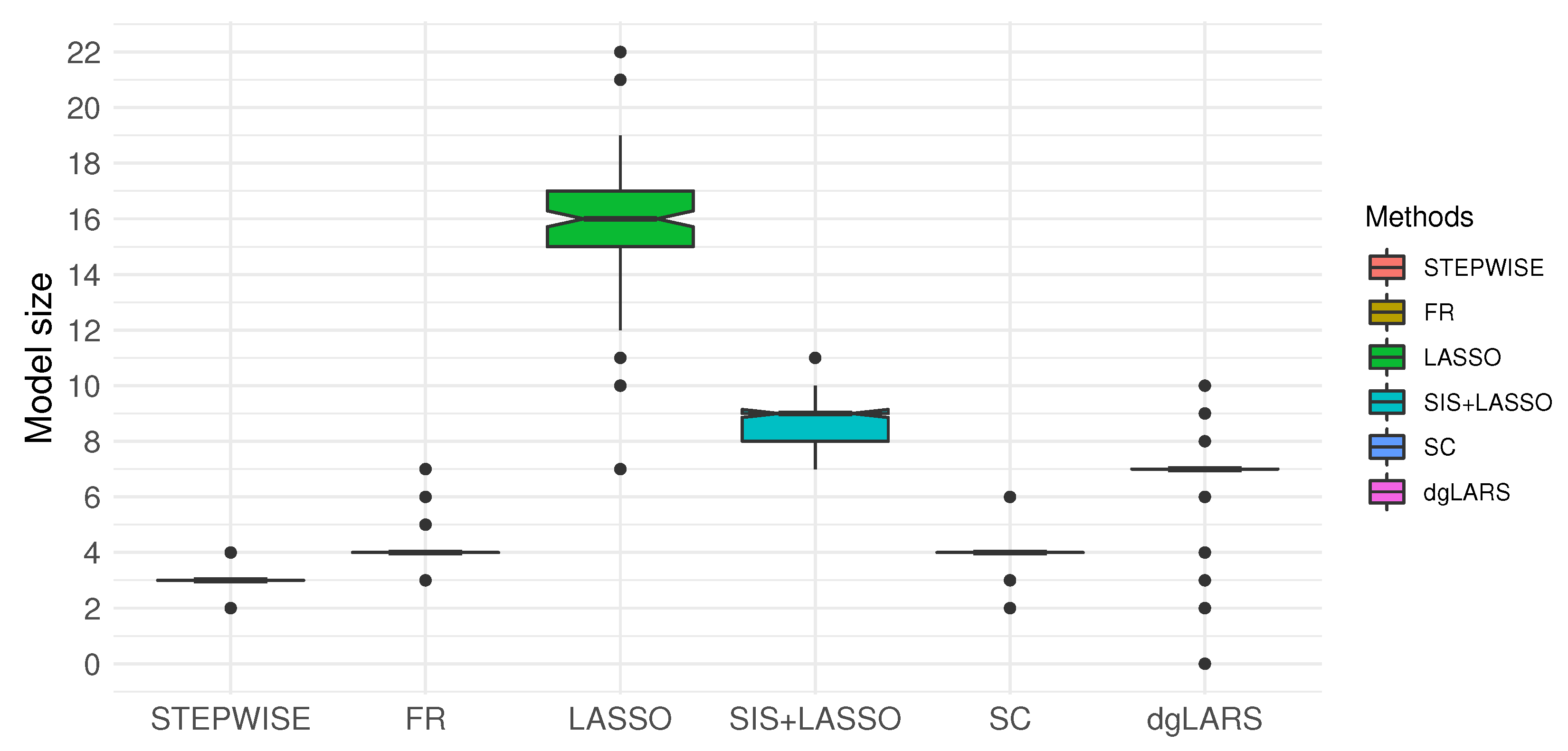
Next, we performed Leave-One-Out Cross-Validation (LOOCV) to obtain the distribution of the model size (MS) and MSPE for the competing methods.

As reported in

Table 5. Comparisons of MSPE among competing methods using the mammalian eye data set.

	STEPWISE	FR	LASSO	SIS+LASSO	SC	dgLARS
Training set	0.005	0.005	0.005	0.006	0.005	0.014
Testing set	0.011	0.012	0.010	0.009	0.014	0.020

Note: The mean squared prediction error (MSPE) was averaged over 120 splits. LASSO, least absolute shrinkage and selection operator with regularization parameter that gives the smallest BIC; SIS+LASSO, sure independence screening by [5] followed by LASSO; dgLARS, differential geometric least angle regression by [11,12] that gives the smallest BIC; SC($\gamma$), sequentially conditioning approach by [8]; FR($\gamma$), forward regression by [7]; STEPWISE, the proposed method. STEPWISE was performed with ${\eta }_1=1$ and ${\eta }_2=4$; FR and SC were performed with $\gamma =1$.

and Figure 1, LASSO, SIS+LASSO and dgLARS tended to select more variables than the forward approaches and STEPWISE. Among all of the methods, STEPWISE selected the fewest variables but with almost the same MSPE as the other methods.

5.2. An Esophageal Squamous Cell Carcinoma Study

Esophageal squamous cell carcinoma (ESCC), the most common histological type of esophageal cancer, is known to be associated with poor overall survival, making early diagnosis crucial for treatment and disease management [37]. Several studies have investigated the roles of circulating microRNAs (miRNAs) in diagnosis of ESCC [38].

Using a clinical study that investigated the roles of miRNAs on the ESCC [39], we aimed to use miRNAs to predict ESCC risks and estimate their impacts on the development of ESCC. Specifically, with a dataset of serum profiling of 2565 miRNAs from 566 ESCC patients and 4965 controls without cancer, we demonstrated the utility of the proposed STEPWISE method in predicting ESCC with miRNAs.

To proceed, we used a balance sampling scheme (283 cases and 283 controls) in the training dataset. The design of yielding an equal number of cases and controls in the training set has proved to be useful [39] for handling imbalanced outcomes as we encountered here. To validate our findings, samples were randomly divided into a training ($n_1=566$, $p=2565$) and testing set ($n_2=4965$, $p=2565$).

The training set consisted of 283 patients with ESCC (median age of 65 years, 79% male) and 283 control patients (median age of 68 years, 46.3% male), and the testing set consisted of 283 patients with ESCC (median age of 67 years, 85.7% male) and 4682 control patients (median age of 67.5 years, 44.5% male). Control patients without ESCC came from three sources: 323 individuals from National Cancer Center Biobank (NCCB); 2670 individuals from the Biobank of the National Center for Geriatrics and Gerontology (NCGG); and 1972 individuals from Minoru Clinic (MC). More detailed characteristics of cases and controls in the training and testing sets are given in

Table 6. Clinicopathological characteristics of study participants of the ESCC data set.

Covariates	Training Set	Testing set
	$n_1$ (%)	$n_2$ (%)
Esophageal squamous cell carcinoma (ESCC) patients
Total number of patients	283	283
Age, median (range)	65 [40, 86]	67 [37, 90]
Gender:
Male	224 (79.0%)	247 (87.3%)
Female	59 (21.0%)	36 (12.7%)
Stage:
0	24 (8.5%)	27 (9.5%)
1	127 (44.9%)	128 (45.2%)
2	58 (20.5%)	57 (20.1%)
3	67 (23.7%)	61 (21.6%)
4	7 (2.4%)	10 (3.6%)
Non-ESCC Controls
Total number of patients	283	4,682
Age, median (range)	68 [27, 92]	67.5 [20, 100]
Gender:
Male	131 (46.3%)	2,086 (44.5%)
Female	152 (53.7%)	2,596 (55.5%)
Data sources of the controls:
National Cancer Center Biobank (NCCB)	17 (6.0%)	306 (6.5%)
National Center for Geriatrics and Gerontology (NCGG)	158 (55.8%)	2,512 (53.7%)
Minoru clinic (MC)	108 (38.2%)	1,864 (39.8%)

.

We defined the binary outcome variable to be 1 if the subject was a case and 0 otherwise. As age and gender (0 = female, 1 = male) are important risk factors for ESCC [40,41] and it is common to adjust for them in clinical models, we set the initial set in STEPWISE to be $F_0=$ {age, gender}. With ${\eta }_1=0$ and ${\eta }_2=3.5$ that were also chosen from 5-fold CV, our procedure recruited three miRNAs. More specifically, miR-4783-3p, miR-320b, miR-1225-3p and miR-6789-5p were selected among 2565 miRNAs by the forward stage from the training set, and then the backward stage eliminated miR-6789-5p.

In comparison, with $\gamma =0$, both FR and SC selected four miRNAs, miR-4783-3p, miR-320b, miR-1225-3p and miR-6789-5p. The list of selected miRNAs by different methods are given in

Table A2. Selected miRNAs for ESCC training dataset.

Methods	Selected miRNAs
STEPWISE	miR-4783-3p; miR-320b; miR-1225-3p
FR	miR-4783-3p; miR-320b; miR-1225-3p; 6789-5p
SC	miR-4783-3p; miR-320b; miR-1225-3p; 6789-5p
LASSO	miR-6789-5p; miR-6781-5p; miR-1225-3p; miR-1238-5p; miR-320b;
	miR-6794-5p; miR-6877-5p; miR-6785-5p; miR-718; miR-195-5p
SIS+LASSO	miR-6785-5p; miR-1238-5p; miR-1225-3p; miR-6789-5p; miR-320b;
	miR-6875-5p; miR-6127; miR-1268b; miR-6781-5p; miR-125a-3p
dgLARS	miR-891b; miR-6127; miR-151a-5p; miR-195-5p; ; miR-3688-5p
	miR-125b-1-3p; miR-1273c; miR-6501-5p; miR-4666a-5p; miR-514a-3p

Note: LASSO, SIS+LASSO, dgLARS selected 20, 17 and 33 miRNAs, respectively, and we only reported top 10 miRNAs.

in Appendix B.

Our findings were biologically meaningful, as the selected miRNAs had been identified by other cancer studies as well. Specifically, miR-320b was found to promote colorectal cancer proliferation and invasion by competing with its homologous miR-320a [42]. In addition, serum levels of miR-320 family members were associated with clinical parameters and diagnosis in prostate cancer patients [43]. Reference [44] showed that miR-4783-3p was one of the miRNAs that could increase the risk of colorectal cancer death among rectal cancer cases. Finally, miR-1225-5p inhibited proliferation and metastasis of gastric carcinoma through repressing insulin receptor substrate-1 and activation of $\beta$-catenin signaling [45].

Aiming to identify a final model without resorting to a pre-screening procedure that may miss out on important biomarkers, we applied STEPWISE to reach the following predictive model for ESCC based on patients’ demographics and miRNAs:

${\mathrm{logit}}^{-1}(-35.70+1.41\times \mathit{miR}-\mathit{4783}-\mathit{3}\mathit{p}+0.98\times \mathit{miR}-\mathit{320}\mathit{b}+1.91\times \mathit{miR}-\mathit{1225}-\mathit{3}\mathit{p}+0.10\times \mathit{Age}-2.02\times \mathit{Gender})$, where ${\mathrm{logit}}^{-1}\left(x\right)=exp\left(x\right)/(1+exp\left(x\right))$.

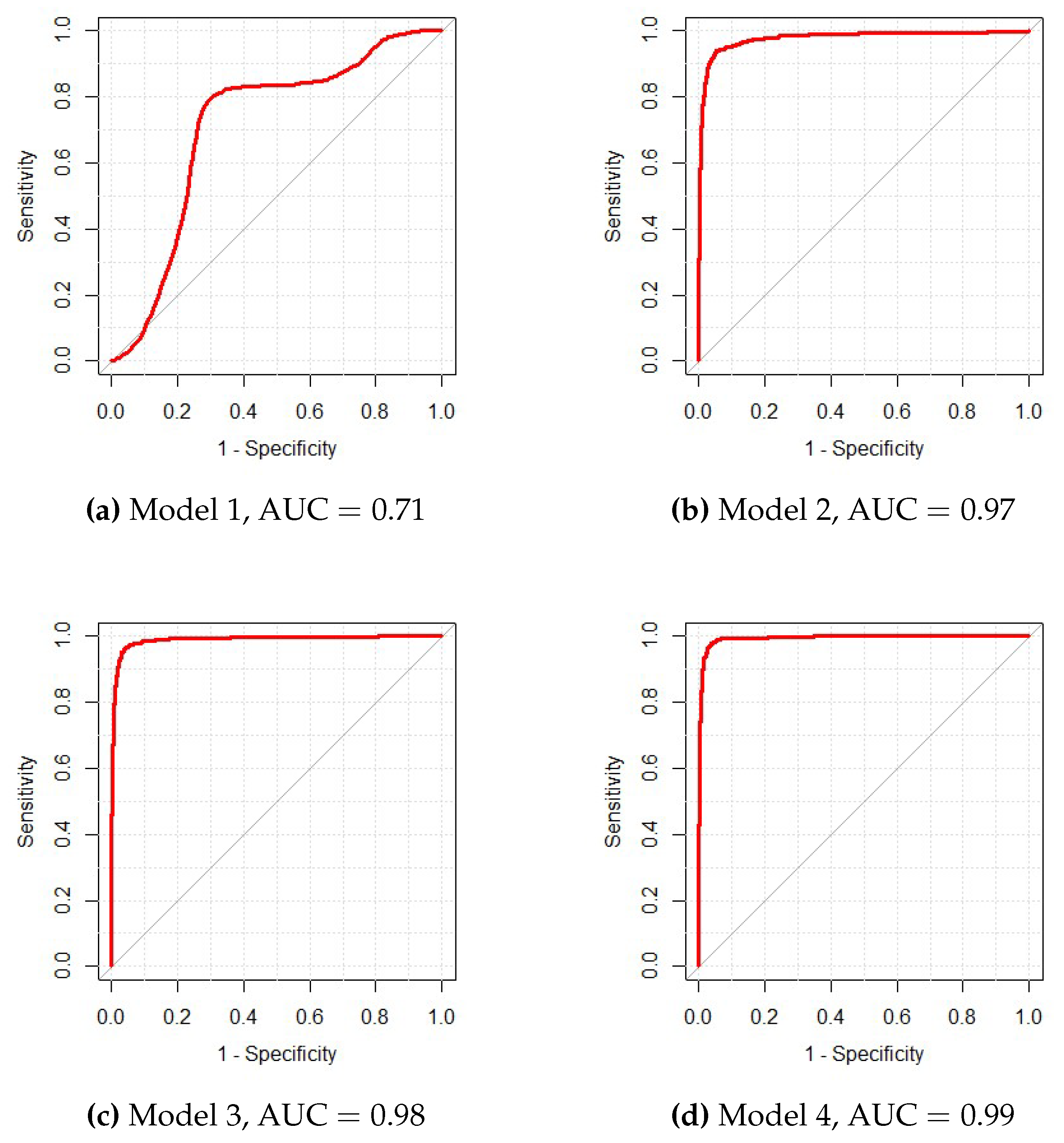
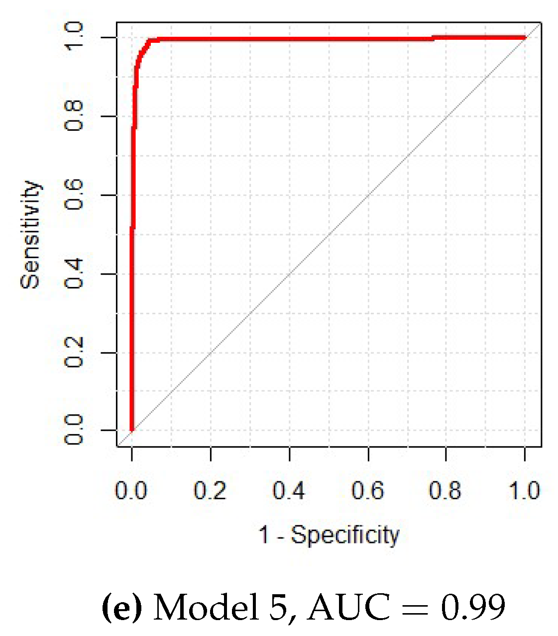
In the testing dataset, the model had an area under the receiver operating curve (AUC) of 0.99 and achieved a high accuracy of 0.96, with a sensitivity and specificity of 0.97 and 0.95, respectively. Additionally, using the testing cohort, we evaluated the performances of the models sequentially selected by STEPWISE. Starting with a model containing age and gender, STEPWISE selected miR-4783-3p, miR-320b and miR-1225-3p in turn. Figure 2, showing the corresponding receiver operating curves (ROC) for these sequential models, revealed the improvement by sequentially adding predictors to the model and justified the importance of these variables in the final model. In addition, Figure 2e illustrated that adding an extra miRNA selected by FR and SC made little improvement of the model’s predictive power.

Furthermore, we conducted subgroup analysis within the testing cohort to study how the sensitivity of the final model differed by cancer stage, one of the most important risk factors. The sensitivities for stages 0, i.e., non-invasive cancer, 9 ($n=27$), 1 ($n=128$), 2 ($n=57$), 3 ($n=61$) and 4 ($n=10$) were 1.00, 0.98, 0.97, 0.97 and 1.00, respectively. We next evaluated how the specificity varied across controls coming from different data sources. The specificities for the various control groups, namely, NCCB ($n=306$), NCGG ($n=2512$) and MC ($n=1864$), were 0.99, 0.99 and 0.98, respectively. The results indicated the robust performance of the miRNA-based model toward cancer stages and data sources.

Finally, to compare STEPWISE with the other competing methods, we repeatedly applied the aforementioned balance sampling procedure and split the ESCC data into the training and testing sets 100 times. We obtained MSPE and the average of accuracy, sensitivity, specificity, and AUC. Figure 3 reported the model size of each method. Though STEPWISE selected fewer variables compared to the other variable selection methods (for example, LASSO selected 11-31 variables and dgLARS selected 12–51 variables), it achieved comparable prediction accuracy, specificity, sensitivity and AUC (see

Table 7. Comparisons of competing methods over 100 independent splits of the ESCC data into training and testing sets.

Training Set	MSPE	Accuracy	Sensitivity	Specificity	AUC
STEPWISE	0.02	0.97	0.98	0.97	1.00
SC	0.01	0.99	0.98	0.98	1.00
FR	0.02	0.99	0.97	0.97	1.00
LASSO	0.01	0.98	1.00	0.97	1.00
SIS+LASSO	0.01	0.99	1.00	0.99	1.00
dgLARS	0.04	0.96	0.99	0.94	1.00
Training Set	MSPE	Accuracy	Sensitivity	Specificity	AUC
STEPWISE	0.04	0.96	0.97	0.95	0.99
SC	0.03	0.96	0.97	0.96	0.99
FR	0.04	0.96	0.97	0.95	0.99
LASSO	0.03	0.96	0.99	0.95	1.00
SIS+LASSO	0.02	0.97	0.99	0.96	1.00
dgLARS	0.05	0.94	0.98	0.94	1.00

Note: Values were averaged over 100 splits. STEPWISE was performed with ${\eta }_1=0$ and ${\eta }_2=1$. SC and FR were performed with $\gamma =1$. The regularization parameters in LASSO and dgLARS were selected to minimize the BIC.

), evidencing the utility of STEPWISE for generating parsimonious models while maintaining competitive predictability.

We used R software [46] to obtain the numerical results in Section 4 and Section 5 with following packages: ggplot2 [47], ncvreg [32], glmnet [31], dglars [34] and screening [33].

6. Discussion

We have proposed to apply STEPWISE to produce final models in ultrahigh dimensional settings, without resorting to a pre-screening step. We have shown that the method identifies or includes the true model with probability going to 1, and produces consistent coefficient estimates, which are useful for properly interpreting the actual impacts of risk factors. The theoretical properties of STEPWISE were established under mild conditions, which are worth discussing. As in practice covariates are often standardized for various reasons, Condition (2) is assumed without loss of generality. Conditions (3) and (4) are generally satisfied under common GLM models, including Gaussian, binomial, Poisson and gamma distributions. Condition (5) is also often satisfied in practice. Proposition 2 in [26] may be used as a tool to verify Condition (5) as well. Conditions (1) and (6) are in good faith with the unknown true model size $\left|\mathcal{M}\right|$ and minimum signal strength $n^{-\alpha }$ in practice. The "irrepresentable" condition (6) is strong and may not hold in some real datasets, see, e.g., [48,49]. However, the condition holds under some commonly used covariance structures, including AR(1) and compound symmetry structure [48].

As shown in simulation studies and real data analyses, STEPWISE tends to generate models as predictive as the other well-known methods, with fewer variables (Figure 3). Parsimonious models are useful for biomedical studies as they explain data with a small number of important predictors, and offer practitioners a realistic list of biomarkers to investigate. With categorical outcome data frequently observed in biomedical studies (e.g., histology types of cancer), STEPWISE can be extended to accommodate multinomial classification, with more involved notation and computation. We will pursue this elsewhere.

There are several open questions. First, our final model was determined by using (E)BIC, which involves two extra parameters ${\eta }_1$ and ${\eta }_2$. In our numerical experiments, we used cross-validation to choose them, which seemed to work well. However, more in-depth research is needed to find their optimal values to strike a balance between false positives and false negatives. Second, despite our consistent estimates, drawing inferences based on them remains challenging. Statistical inference, which accounts for uncertainty in estimation, is key for properly interpreting analysis results and drawing appropriate conclusions. Our asymptotic results, nevertheless, are a stepping stone toward this important problem.

References

- Prosperi, M.; Min, J.S.; Bian, J.; Modave, F. Big data hurdles in precision medicine and precision public health. BMC Med. Inform. Decis. Mak. 2018, 18, 139. [Google Scholar] [CrossRef] [PubMed]
- Tibshirani, R. Regression shrinkage and selection via the lasso. J. R. Stat. Soc. Ser. B-Stat. Methodol. 1996, 58, 267–288. [Google Scholar] [CrossRef]
- Flynn, C.J.; Hurvich, C.M.; Simonoff, J.S. On the sensitivity of the lasso to the number of predictor variables. Stat. Sci. 2017, 32, 88–105. [Google Scholar] [CrossRef] [Green Version]
- van de Geer, S.A. On the asymptotic variance of the debiased Lasso. Electron. J. Stat. 2019, 13, 2970–3008. [Google Scholar] [CrossRef]
- Fan, J.; Lv, J. Sure independence screening for ultrahigh dimensional feature space (with discussion). J. R. Stat. Soc. Ser. B-Stat. Methodol. 2008, 70, 849–911. [Google Scholar] [CrossRef] [Green Version]
- Barut, E.; Fan, J.; Verhasselt, A. Conditional sure independence screening. J. Am. Stat. Assoc. 2016, 111, 1266–1277. [Google Scholar] [CrossRef] [PubMed]
- Wang, H. Forward regression for ultra-high dimensional variable screening. J. Am. Stat. Assoc. 2009, 104, 1512–1524. [Google Scholar] [CrossRef]
- Zheng, Q.; Hong, H.G.; Li, Y. Building generalized linear models with ultrahigh dimensional features: A sequentially conditional approach. Biometrics 2019, 76, 1–14. [Google Scholar] [CrossRef]
- Hong, H.G.; Zheng, Q.; Li, Y. Forward regression for Cox models with high-dimensional covariates. J. Multivar. Anal. 2019, 173, 268–290. [Google Scholar] [CrossRef]
- Efron, B.; Hastie, T.; Johnstone, I.; Tibshirani, R. Least angle regression. Ann. Stat. 2004, 32, 407–499. [Google Scholar]
- Augugliaro, L.; Mineo, A.M.; Wit, E.C. Differential geometric least angle regression: A differential geometric approach to sparse generalized linear models. J. R. Stat. Soc. Ser. B-Stat. Methodol. 2013, 75, 471–498. [Google Scholar] [CrossRef] [Green Version]
- Pazira, H.; Augugliaro, L.; Wit, E. Extended differential geometric LARS for high-dimensional GLMs with general dispersion parameter. Stat. Comput. 2018, 28, 753–774. [Google Scholar] [CrossRef]
- An, H.; Huang, D.; Yao, Q.; Zhang, C.H. Stepwise Searching for Feature Variables in High-Dimensional Linear Regression. 2008. Available online: http://eprints.lse.ac.uk/51349/ (accessed on 20 August 2020).
- Ing, C.K.; Lai, T.L. A stepwise regression method and consistent model selection for high-dimensional sparse linear models. Stat. Sin. 2011, 21, 1473–1513. [Google Scholar] [CrossRef] [Green Version]
- Hwang, J.S.; Hu, T.H. A stepwise regression algorithm for high-dimensional variable selection. J. Stat. Comput. Simul. 2015, 85, 1793–1806. [Google Scholar] [CrossRef]
- McCullagh, P. Generalized Linear Models; Routledge: Abingdon-on-Thames, UK, 1989. [Google Scholar]
- Chen, J.; Chen, Z. Extended BIC for small-n-large-P sparse GLM. Stat. Sin. 2012, 22, 555–574. [Google Scholar] [CrossRef] [Green Version]
- Bühlmann, P.; Yu, B. Sparse boosting. J. Mach. Learn. Res. 2006, 7, 1001–1024. [Google Scholar]
- van de Geer, S.A. High-dimensional generalized linear models and the lasso. Ann. Stat. 2008, 36, 614–645. [Google Scholar] [CrossRef]
- Chen, J.; Chen, Z. Extended Bayesian information criteria for model selection with large model spaces. Biometrika 2008, 95, 759–771. [Google Scholar] [CrossRef] [Green Version]
- Fan, Y.; Tang, C.Y. Tuning parameter selection in high dimensional penalized likelihood. J. R. Stat. Soc. Ser. B-Stat. Methodol. 2013, 75, 531–552. [Google Scholar] [CrossRef] [Green Version]
- Cheng, M.Y.; Honda, T.; Zhang, J.T. Forward variable selection for sparse ultra-high dimensional varying coefficient models. J. Am. Stat. Assoc. 2016, 111, 1209–1221. [Google Scholar] [CrossRef] [Green Version]
- Zhao, S.D.; Li, Y. Principled sure independence screening for Cox models with ultra-high-dimensional covariates. J. Multivar. Anal. 2012, 105, 397–411. [Google Scholar] [CrossRef] [PubMed] [Green Version]
- Kwemou, M. Non-asymptotic oracle inequalities for the Lasso and group Lasso in high dimensional logistic model. ESAIM-Prob. Stat. 2016, 20, 309–331. [Google Scholar] [CrossRef]
- Jiang, Y.; He, Y.; Zhang, H. Variable selection with prior information for generalized linear models via the prior LASSO method. J. Am. Stat. Assoc. 2016, 111, 355–376. [Google Scholar] [CrossRef]
- Zhang, C.H.; Huang, J. The sparsity and bias of the Lasso selection in high-dimensional linear regression. Ann. Stat. 2008, 36, 1567–1594. [Google Scholar] [CrossRef]
- Fan, J.; Song, R. Sure independence screening in generalized linear models with NP-dimensionality. Ann. Stat. 2010, 38, 3567–3604. [Google Scholar] [CrossRef]
- Luo, S.; Chen, Z. Sequential Lasso cum EBIC for feature selection with ultra-high dimensional feature space. J. Am. Stat. Assoc. 2014, 109, 1229–1240. [Google Scholar] [CrossRef]
- Luo, S.; Xu, J.; Chen, Z. Extended Bayesian information criterion in the Cox model with a high-dimensional feature space. Ann. Inst. Stat. Math. 2015, 67, 287–311. [Google Scholar] [CrossRef]
- Hastie, T.; Tibshirani, R.; Friedman, J. The Elements of Statistical Learning: Data mining, Inference, and Prediction; Springer: Berlin/Heidelberger, Germany, 2009. [Google Scholar]
- Simon, N.; Friedman, J.; Hastie, T.; Tibshirani, R. Regularization Paths for Cox’s Proportional Hazards Model via Coordinate Descent. J. Stat. Softw. 2011, 39, 1–13. [Google Scholar] [CrossRef]
- Breheny, P.; Huang, J. Coordinate descent algorithms for nonconvex penalized regression, with applications to biological feature selection. Ann. Appl. Stat. 2011, 5, 232–253. [Google Scholar] [CrossRef] [Green Version]
- Wang, X.; Leng, C. R Package: Screening. 2016. Available online: https://github.com/wwrechard/screening (accessed on 20 August 2020).
- Augugliaro, L.; Mineo, A.M.; Wit, E.C. dglars: An R Package to Estimate Sparse Generalized Linear Models. J. Stat. Softw. 2014, 59, 1–40. [Google Scholar] [CrossRef] [Green Version]
- Scheetz, T.E.; Kim, K.Y.A.; Swiderski, R.E.; Philp, A.R.; Braun, T.A.; Knudtson, K.L.; Dorrance, A.M.; DiBona, G.F.; Huang, J.; Casavant, T.L.; et al. Regulation of gene expression in the mammalian eye and its relevance to eye disease. Proc. Natl. Acad. Sci. USA 2006, 103, 14429–14434. [Google Scholar] [CrossRef] [PubMed] [Green Version]
- Chiang, A.P.; Beck, J.S.; Yen, H.J.; Tayeh, M.K.; Scheetz, T.E.; Swiderski, R.E.; Nishimura, D.Y.; Braun, T.A.; Kim, K.Y.A.; Huang, J.; et al. Homozygosity mapping with SNP arrays identifies TRIM32, an E3 ubiquitin ligase, as a Bardet–Biedl syndrome gene (BBS11). Proc. Natl. Acad. Sci. USA 2006, 103, 6287–6292. [Google Scholar] [CrossRef] [PubMed] [Green Version]
- He, S.; Peng, J.; Li, L.; Xu, Y.; Wu, X.; Yu, J.; Liu, J.; Zhang, J.; Zhang, R.; Wang, W. High expression of cytokeratin CAM5.2 in esophageal squamous cell carcinoma is associated with poor prognosis. Medicine 2019, 98, e17104. [Google Scholar] [CrossRef]
- Li, B.X.; Yu, Q.; Shi, Z.L.; Li, P.; Fu, S. Circulating microRNAs in esophageal squamous cell carcinoma: Association with locoregional staging and survival. Int. J. Clin. Exp. Med. 2015, 8, 7241–7250. [Google Scholar]
- Sudo, K.; Kato, K.; Matsuzaki, J.; Boku, N.; Abe, S.; Saito, Y.; Daiko, H.; Takizawa, S.; Aoki, Y.; Sakamoto, H.; et al. Development and validation of an esophageal squamous cell carcinoma detection model by large-scale microRNA profiling. JAMA Netw. Open 2019, 2, e194573. [Google Scholar] [CrossRef] [Green Version]
- Zhang, Y. Epidemiology of esophageal cancer. World J. Gastroenterol 2013, 19, 5598–5606. [Google Scholar] [CrossRef]
- Mathieu, L.N.; Kanarek, N.F.; Tsai, H.L.; Rudin, C.M.; Brock, M.V. Age and sex differences in the incidence of esophageal adenocarcinoma: Results from the Surveillance, Epidemiology, and End Results (SEER) Registry (1973–2008). Dis. Esophagus 2014, 27, 757–763. [Google Scholar] [CrossRef]
- Zhou, J.; Zhang, M.; Huang, Y.; Feng, L.; Chen, H.; Hu, Y.; Chen, H.; Zhang, K.; Zheng, L.; Zheng, S. MicroRNA-320b promotes colorectal cancer proliferation and invasion by competing with its homologous microRNA-320a. Cancer Lett. 2015, 356, 669–675. [Google Scholar] [CrossRef] [Green Version]
- Lieb, V.; Weigelt, K.; Scheinost, L.; Fischer, K.; Greither, T.; Marcou, M.; Theil, G.; Klocker, H.; Holzhausen, H.J.; Lai, X.; et al. Serum levels of miR-320 family members are associated with clinical parameters and diagnosis in prostate cancer patients. Oncotarget 2018, 9, 10402–10416. [Google Scholar] [CrossRef] [Green Version]
- Mullany, L.E.; Herrick, J.S.; Wolff, R.K.; Stevens, J.R.; Slattery, M.L. Association of cigarette smoking and microRNA expression in rectal cancer: Insight into tumor phenotype. Cancer Epidemiol. 2016, 45, 98–107. [Google Scholar] [CrossRef] [Green Version]
- Zheng, H.; Zhang, F.; Lin, X.; Huang, C.; Zhang, Y.; Li, Y.; Lin, J.; Chen, W.; Lin, X. MicroRNA-1225-5p inhibits proliferation and metastasis of gastric carcinoma through repressing insulin receptor substrate-1 and activation of β-catenin signaling. Oncotarget 2016, 7, 4647–4663. [Google Scholar] [CrossRef] [Green Version]
- R Core Team. R: A Language and Environment for Statistical Computing; R Foundation for Statistical Computing: Vienna, Austria, 2018. [Google Scholar]
- Wickham, H. ggplot2: Elegant Graphics for Data Analysis; Springer: Berlin/Heidelberger, Germany, 2016. [Google Scholar]
- Zhao, P.; Yu, B. On model selection consistency of Lasso. J. Mach. Learn. Res. 2006, 7, 2541–2563. [Google Scholar]
- Bühlmann, P.; Van De Geer, S. Statistics for High-dimensional Data: Methods, Theory and Applications; Springer: Berlin/Heidelberger, Germany, 2011. [Google Scholar]
- Vaart, A.W.; Wellner, J.A. Weak Convergence and Empirical Processes: With Applications to Statistics; Springer: Berlin/Heidelberger, Germany, 1996. [Google Scholar]
- Talagrand, M. Sharper bounds for Gaussian and empirical processes. Ann. Probab. 1994, 22, 28–76. [Google Scholar] [CrossRef]
Figure 1.
Box plot of model sizes for each method over 120 different training samples from the mammalian eye data set. STEPWISE was performed with and , and FR and SC were conducted with .
Figure 2.
Comparisons of ROC curves for the selected models in the ESCC data set by the sequentially selected order: Model 1: ; Model 2: miR-4783-3p; Model 3: miR-4783-3pmiR-320b; Model 4: miR-4783-3pmiR-320bmiR-1225-3p; Model 5: miR-4783-3pmiR-320bmiR-1225-3p miR-6789-5p.
Figure 3.
Box plot of model sizes for each method based on 100 ESCC training datasets. Performance of STEPWISE is reported with and . Performances of SC and FR are reported with .