
Convergence of Coupling-Parameter Expansion-Based Solutions to Ornstein–Zernike Equation in Liquid State Theory


Shiv Enclave, 304, 31-B-Wing, Tilak Nagar, Mumbai 400089, India
†
Retired from Bhabha Atomic Research Centre, Mumbai 400085, India.
Condens. Matter 2021, 6(3), 29; https://doi.org/10.3390/condmat6030029
Submission received: 5 June 2021
/
Revised: 31 July 2021
/
Accepted: 2 August 2021
/
Published: 5 August 2021
(This article belongs to the Section Condensed Matter Theory)
Abstract
:The objective of this paper is to investigate the convergence of coupling-parameter expansion-based solutions to the Ornstein–Zernike equation in liquid state theory. The analytically solved Baxter’s adhesive hard sphere model is analyzed first by using coupling-parameter expansion. It was found that the expansion provides accurate approximations to solutions—including the liquid-vapor phase diagram—in most parts of the phase plane. However, it fails to converge in the region where the model has only complex solutions. Similar analysis and results are obtained using analytical solutions within the mean spherical approximation for the hardcore Yukawa potential. However, numerical results indicate that the expansion converges in all regions in this model. Next, the convergence of the expansion is analyzed for the Lennard-Jones potential by using an accurate density-dependent bridge function in the closure relation. Numerical results are presented which show convergence of correlation functions, compressibility versus density profiles, etc., in the single as well as two-phase regions. Computed liquid-vapor phase diagrams, using two independent schemes employing the converged profiles, compare excellently with simulation data. The results obtained for the generalized Lennard-Jones potential, with varying repulsive exponent, also compare well with the simulation data. Solution-spaces and the bifurcation of the solutions of the Ornstein–Zernike equation that are relevant to coupling-parameter expansion are also briefly discussed. All of these results taken together establish the coupling-parameter expansion as a practical tool for studying single component fluid phases modeled via general pair-potentials.
1. Introduction
Liquid state theory deals with correlation functions, such as the pair-distribution function, to describe the structural and thermodynamics properties of fluids [1]. The correlation functions also form the basis of the modern theory of phase transitions in fluid systems [2]. The Ornstein–Zernike equation (OZE), which relates the direct and total correlation functions, is known to have excellent predictive power when supplemented with appropriate closure relations. The latter, as the name suggests, relates the two correlation functions and the interaction pair-potential. Although there are no exact closure relations, very accurate relations available in the literature provide results which compare excellently with those from computer simulations for homogeneous fluids [3]. There are also approaches wherein empirically introduced parameters in closure relations are tuned so as to impose thermodynamic consistency [4].
For realistic interaction potentials and accurate closure relations, the OZE is a highly non-linear integral equation, which is numerically solved using Newton’s method [5]. This approach works quite effectively for the case of purely repulsive interaction potentials [6]. However, a number of investigations show that the situation is quite different below the liquid-vapor phase transition temperature, which arises whenever there is an attractive component in the potential. Even simple models show the occurrence of multiple solutions and ‘no-real-solution-region’ in the liquid-vapor coexistence region [7]. This feature is most clearly illustrated in Baxter’s analytical solution of the adhesive hard sphere (AHS) model [8], which shows multiple solutions even with the diverging pair distribution function. The model employs the Percus–Yevick (PY) closure for hard spheres with adhesion. The proper solution branch from multiple solutions is easily selected so as to satisfy the ideal gas limit and spatial convergence of the pair distribution function. However, the model shows the emergence of a density domain in the two-phase region where all solutions are complex. It also shows the absence of a true spinodal line on the vapor side of the phase plane. Numerical methods also show similar features for the Lennard-Jones (LJ) potential and several important closure relations [9]. However, by using a different numerical technique with the PY closure, unique real solutions in the stable and metastable regions and multiple real solutions in the unstable (spinodal) region are also obtained [10]. It is difficult to enumerate all solution branches with any numerical scheme. On the other hand, analytical solutions within the mean spherical approximation (MSA) for the hardcore Yukawa (HCY) potential show the occurrence of two real and two complex solutions in the entire phase-plane. More specifically, it was found that there is a domain in the two-phase region where all solutions are complex. The model shows proper spinodal-lines on the vapor and liquid sides [11], as in van der Waals model and other mean field theories. Fortunately, the ‘no-real-solution-region’ in all models occurs inside the liquid-vapor coexistence dome, and careful strategies can be designed to map out the boundaries of the dome from numerical solutions of OZE [12].
An alternate approach to obtain useful approximations to fluid correlation functions is the thermodynamic perturbation theory (TPT) [13]. Here, the basic idea is to use the known (or accurately calculable) solutions for a reference potential and to incorporate the effects of perturbing potential via correction terms. Perturbation theories based purely on the fluid free energy mostly use the hard sphere model as the reference system [14]. This is because of the availability of simulation data on hard sphere systems in very accurate parameter forms [13]. While first order correction terms are easily computed by using the pair distribution function of the hard sphere system, three and four particle correlation functions are required even for second order term. Thus, the conventional TPT is restricted to low orders. The possibility of using OZE in higher order perturbation theory avoids the requirement of complicated correlation functions; however, it requires the computation of higher order derivative terms of the correlation functions [15]. A systematic development of this approach, called coupling-parameter expansion (CPE), to arbitrary high orders has provided good results for model systems in comparison to simulation data [16]. One of the most appropriate divisions of molecular potentials to reference and perturbing parts is based on the Weeks–Chandler–Andersen (WCA) prescription [17]. Recently, the CPE that employs this division and also incorporating density-dependent bridge functions is developed as a general method, making use of efficient Newton–Armijo and Krylov space-based solvers [18]. It has also been applied to compute phase diagrams of metallic fluids using effective pair-potentials derived from cohesive energy curves. However, there remains an important issue related to convergence of the CPE.
The main objective of the paper is to obtain results on the convergence of CPE, in particular, the two-phase region where OZE shows the occurrence of multiple and complex solutions. In what follows, CPE is first described briefly. Subsequently, its convergence is analyzed by using the analytical solutions for AHS and MSA-HCY systems. Important conclusions on convergence are obtained in this manner. Then, numerical results are obtained by using the general scheme for the LJ potential, which show convergence near the critical isotherm, and even in the two-phase region. A phase diagram of the LJ system is obtained via two independent schemes. Finally, the method is applied to generate the phase-diagrams for the general LJ(n,6) potentials and compared with simulation data. Important issues related to solution-spaces and bifurcation of solutions of OZE, which are relevant to coupling-parameter expansion, are also briefly discussed. The overall conclusion emerging from this analysis is that CPE is a practical approach for obtaining thermodynamic properties of one-component fluids interacting via general potentials. Thermodynamic models of fluid properties, particularly in the two-phase region, are essential in applications involving equations of state of liquid metals [19,20], which are important in high pressure physics. It is expected that CPE will find good use in generating the equations of state data [21] in the fluid domain.
2. Coupling-Parameter Expansion—General
The first step in introducing the general CPE [18] is to divide the inter-particle potential into a reference (purely repulsive) and perturbation (purely attractive) components employing the WCA prescription [17]. These components are given by the following.
Here, denotes the potential-minimum at position . The purely repulsive part determines the structure of dense liquids while the attractive perturbing component gives rise to cohesion and phase changes [17]. When the coupling-parameter is introduced into the potential, it reads as . The magnitude of , which varies over , determines the strength of the perturbation; thus, is the reference part and the full potential. Now, all correlation functions which determine the structure and thermodynamic properties of the fluid are also to be considered as functions of . In TPT, these functions are expanded as Taylor’s series in about their reference part. For example, the pair distribution function is expanded as follows.
Here, is the reference system’s pair distribution function and denotes the derivatives of at . Similarly, Taylor’s series expansions are also assumed for other correlation functions: the direct correlation function , the total correlation function , and the indirect correlation function . The subscript 0 in these functions denotes their corresponding functions for the reference system. The basic assumption in CPE is that these expansions converge and the series can be truncated at a suitable order. Thus, the main idea is that the contributions from the perturbing part of potential are accurately accounted for via the derivatives such as . While traditional perturbation theory is limited to the first two orders [13], the general formulation of CPE can incorporate quite higher order derivatives by taking recourse to the OZE.
The OZE defines the consistency relation between the short ranged direct correlation function and the long ranged total correlation function . Similar to the pair-potential, both these functions tend to zero for large r. For one-component systems modeled using spherically symmetric potentials, the OZE is written as follows:
where is the number density of fluid particles. This is one equation in two unknowns, and it needs to be supplemented with a closure relation involving and and the pair-potential . An exact closure is unfeasible; however, several approximate forms are available [1]. All the closures are generally expressed concisely in terms of a ‘bridge function’ in the following form:
where , is Boltzmann’s constant, and T denotes absolute temperature. Approximate forms of generate different closures; for instance, yields the PY closure while the hypernetted-chain closure (HNC) is obtained with . A bridge function applicable to general potentials [22] is as follows:
which will be used throughout the present paper. Here and throughput the paper, is a dimensionless number density. This function has been shown to provide accurate thermodynamic properties for hard sphere as well as LJ systems.
2.1. Method of Solution
The solution of integral equation Equation (3) with a displacement kernel in Fourier space is easily expressed as follows:
where the Fourier transform (denoted with a ‘bar’ throughout) and its inverse, for any function , are defined as the following.
The algebraic equations Equations (4) and (6), although the first is defined in r-space and the second in k-space, define a closed non-linear system within the integral equation formalism. Different implementations of Newton’s method to solve this system are now well developed [23]. However, they all have to deal with the problems mentioned earlier related to the ‘no-real-solution-region’ in the two-phase region.
In CPE, the Newton–Armijo solver is employed only for determining correlation functions of reference part. Starting with an initial guess (hence, , , and ), a correction is obtained by solving the following linear integral equation [18].
Here, is the derivative of the bridge function , defined in Equation (5), at . Fourier transforms and inverses are computed by using FFT (fast-Fourier-transform) algorithms. The linear integral equation implicitly defined in Equation (8) is best solved with Krylov space-based methods such as CGNR (Conjugate Gradient to Normal equations to minimize Residual) or GMRES (Generalized Minimum Residual). This is because it is possible to perform matrix-vector products via two Fourier transform operations. The Armijo scheme is used to limit the correction to with in case error reduction does not occur at any iteration.
The derivatives of correlation functions are obtained from the solutions of the system of lineal integral equations.
Here, denotes the structure factor of the reference system. By denoting the derivatives of the bridge function also as , the source terms, viz., and , are given by the following.
Here, denotes the binomial coefficient. Note that the terms on right side involve only lower order derivatives, and, hence, are known at the nth order. Furthermore, the linear operator in Equation (9) (for all orders) is identical to that in Equation (8). Finally, the derivatives are expressed as follows.
As the summation contributes only for , this equation provides explicitly at all orders. Derivations of these expressions are given in detail in the recent formulation of CPE mentioned earlier [18]. Concise algorithms for implementing the complete CPE method are also discussed there. (Note that the line in Algorithm A5 provided in this reference should be corrected as .)
2.2. Thermodynamic Functions
Once the derivatives are determined to the required order, explicit expressions for the correlation functions follow as functions of . Then, the series for provides an explicit expression for free energy F per particle [24].
Here, is free energy per particle of the reference system. With the series expansion for , the integral term over is evaluated as . By using the closure relation, which is also expressed as , the above expression is recast as follows [24].
Here, the subscript in (and similarly other functions) denotes the excess contribution over that of the reference potential, i.e., . This form does not involve the attractive potential explicitly. Again, the integral term over is obtained as . Once is determined, pressure and chemical potential are readily computed. It is to be noted that this approach does not require integration over density or temperature.
The thermodynamic properties are also be obtained via the compressibility route. The (reduced) inverse compressibility is provided in terms of a direct correlation function as follows.
As the function is short ranged, is the most appropriate response function for computing pressure on an isotherm via integration with respect to , whenever possible. Tje chemical potential is also determined by integrating the thermodynamic equation , as follows.
The first two terms, where is the thermal wavelength, are the ideal gas contributions. This approach is always useful for computing for the reference system and is employed in this paper. There are also explicit expressions for virial-pressure and chemical potential [12], involving , , and .
Having outlined the general algorithm for CPE, numerical investigations of convergence of the expansion for specific potentials are readily carried out. Before that, this analysis is conducted using analytical solutions of two model problems in the next two sections.
3. Coupling Parameter Expansion—AHS Model
Baxter’s AHS model deals with a system of hard spheres (of diameter ) with an infinitely narrow attractive square well potential (of width ) representing surface adhesion [8]. The well depth is taken as , where the parameter represents an effective temperature, being zero at zero temperature and large at high temperatures. In the limit , this particular form reduces Mayer’s function to the form = −1 + , where −1 represents the hard sphere contribution. By using virial expansion, it is also shown that the total correlation function reduces to = −1 + for the range , where is a parameter to be determined employing OZE and PY closure. Baxter showed that = (1−) satisfies the following quadratic equation:
where is the volume fraction of particles. This equation shows that the solutions are real in the entire range when . However, they turn complex for a range around when . These boundaries are determined from the condition of vanishing discriminant in Equation (16), viz., . Thus the model predicts a gas-liquid phase transition with critical parameters and . The proper root out of the two solutions that satisfy the ideal gas limit (for small ) is the negative root given by the following.
The analytical expression for pressure [8] that is obtained by integrating compressibility for , and analytically continued to is given by the following.
Here, the first term is the compressibility-pressure for hard spheres within the PY closure. Other terms involving are the contributions of surface adhesion. Similar expressions for chemical potential is also derived [25], and these expressions facilitate the determination of phase diagram [25] by using thermodynamic conditions. It is nice to note that the ‘no-real-solution-region’, where and, hence, P are undefined, is contained inside the co-existence region (see below). What is equally important is that the model shows the emergence of multiple solutions in all regions and a ‘no-real-solution-region’ in the two-phase region.
The equations of the AHS model are also derived as the lowest order solution to Baxter’s factorized form of OZE [26]. This analysis employed as a perturbation parameter [27] and directly showed that Equation (16) is accurate to and the parameters and are related to square well parameters as the following:
where is the depth of the potential. Now, all results of the model can be discussed in the usual phase-plane as the parameter is explicitly related to T.
The CPE is introduced by replacing the potential depth with . Then, the functions and , which is directly related to , are expanded in a power series as the following.
The series for is uniformly convergent with expansion coefficients for . Substitution from Equations (20) into the quadratic equation, Equation (16), yields the following expansion coefficients :
where satisfies an equation similar to Equation (16) but with in place of .
This equation is similar to the OZE for reference potential while Equation (21) is analogous to the solution of the system of linear integral equations defined in Equation (9). The parameters and correspond to the AHS model for depth but finite and small . This is taken as the reference system in lieu of the hard sphere system, because in order to obtain the hard sphere limit , it will be necessary to take the limit . The coefficients obtained up to sufficient order provides , which yields all thermodynamic properties within CPE. The series expansion for is also derivable from Equation (17). However, by writing the second square bracket term in this expression as , where , this equation shows that the series fails to converge for when , that is, within the ‘no-real-solution-region’.
The convergence properties just discussed are also elaborated in Table 1, where the ratio of the expansion coefficients versus n are given at three volume fractions for the subcritical temperature (see below). The ‘no-real-solution-region’ boundaries for this temperature are and . The volume fractions and lie outside this region while lies inside. First and third columns illustrate convergence of CPE series, whereas the second column indicates a non-convergent series for . Thus, the real values of obtained in the ‘no-real-solution-region’ at any order of truncation do not correspond to convergent series. However, this is not a serious issue, as will be discussed below.
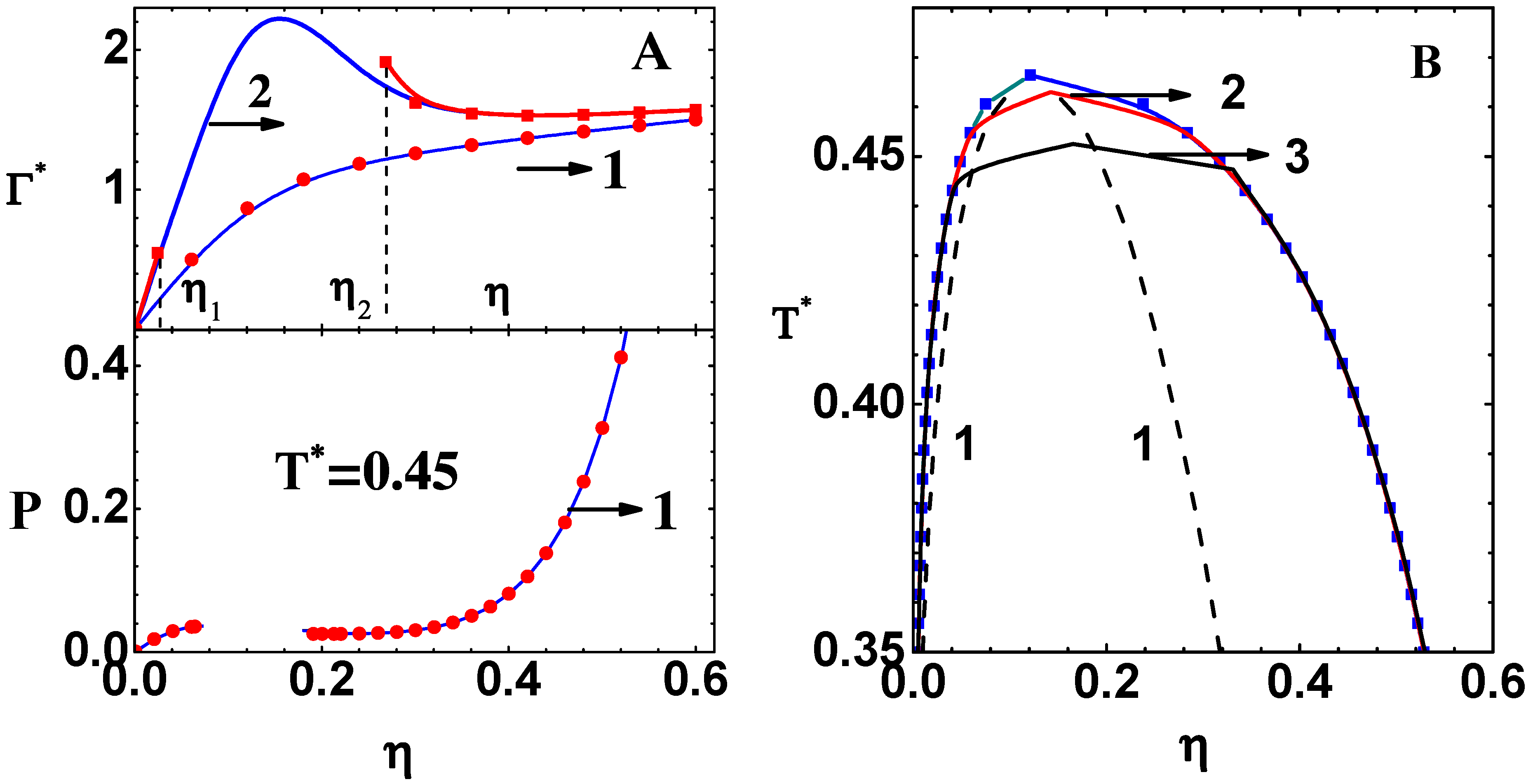
The variation of versus is compared with the exact solution (see Equation (17)) in Figure 1A (upper part) for two values of reduced temperature . These results correspond to the perturbation (width) parameter , which yields the critical temperature . Graph of versus obtained using CPE of 20th order (curve-1) and exact results (symbols) compare excellently, and this case corresponds to . Similar comparisons are found even at the 10th order. In the case of , the range is the ‘no-real-solution-region’. Again, versus from CPE of 20th order (curve-2) and the exact results (symbols) are compared. There are deviations between the two sets of results in the neighborhood of and , otherwise they agree quite well. The portion of graph for obtained via CPE does not correspond to a convergent series. A subcritical isotherm for obtained via the compressibility route in CPE (curve-1) and the exact results (symbols) are compared in the lower part. Excellent agreement is found once again between the two sets of results, except in the ‘no-real-solution-region’ (blank portion). Similar agreement is obtained for chemical potential as well. Next, the phase diagram of AHS model is computed by using the analytical expressions for P and in the thermodynamic conditions, viz., and , where the subscripts L and G, respectively, denote the liquid and gaseous branches. The exact results for the phase diagram (blue line and symbols) are compared in Figure 1B with those obtained by using CPE of 50th order (curve-2) and 20th order (curve-3). These agree with one another, except for when it is close to the critical point. Critical temperature obtained at these orders are and , respectively. The ‘no-real-solution-region’, lying within the dashed lines (curve-1), is also shown. These comparisons show that CPE provides useful results because the ‘no-real-solution-region’ where the expansion fails to converge lies completely inside the co-existence dome.
4. Coupling Parameter Expansion—MSA Model
The system of hard spheres (of diameter ) attached with the attractive Yukawa potential is analytically solved within the MSA closure [28]. The Yukawa part, defined over the range , is expressed as , where and J are range and depth parameters, respectively. Analytical results of the model are useful for analyzing the convergence properties of CPE. Explicit expressions for all thermodynamic quantities exist in terms of a parameter ; for instance, the reduced compressibility is obtained as follows:
where is an explicit function of and volume fraction . Similar expressions are also derived for pressure computed via the virial and energy routes [11]. The central parameter of the model satisfies a fourth degree polynomial equation of the following:
where and X and Y are specified functions of and . Note that this model has more solutions compared to the AHS model. This equation has two real and two complex solutions in the entire range of for K (proportional to ) lower than a critical value . Out of the two real solutions, the proper one must approach the ideal gas limit for small and should also vanish as . For the region , there is a ‘no-real-solution-region’ for a range , because all solutions turn complex. Thus, the results of the model, although there are more solutions, are similar to those of the AHS model. However, an important difference is that the spinodal lines, which now occur on both the gaseous and liquid branches, encompass the ‘no-real-solution-region’. Thus, the occurrence of the latter may not be of much consequence in determining the phase diagram.
The CPE is introduced in the model by replacing K with . Then the reference solution is that of hard spheres within the PY closure. As the proper real solution must approach zero as , the series expansion for must start at first order and is given by the following.
Recursion relations for the expansion coefficients readily follow on substituting this series in Equation (24):
where the additional coefficients , , and are obtained as the following.
After truncating the expansion at a suitable order, is to be substituted in the analytical expressions [11] to obtain the results within CPE. Note that CPE generates real solutions for all values of and K.
The convergence properties of CPE in the MSA-HCY model is different from that of the AHS model. The ratios of the expansion coefficients versus n are given in Table 2 for three volume fractions for , which is in the subcritical range (see below). Volume fraction and lie outside the ‘no-real-solution-region’, while lies inside (see upper portion in Figure 2A). However, the data in this table illustrates convergence of CPE for all three . Similar results are obtained for as well. Thus, CPE converges even the ‘no-real solution-region’ in this model.
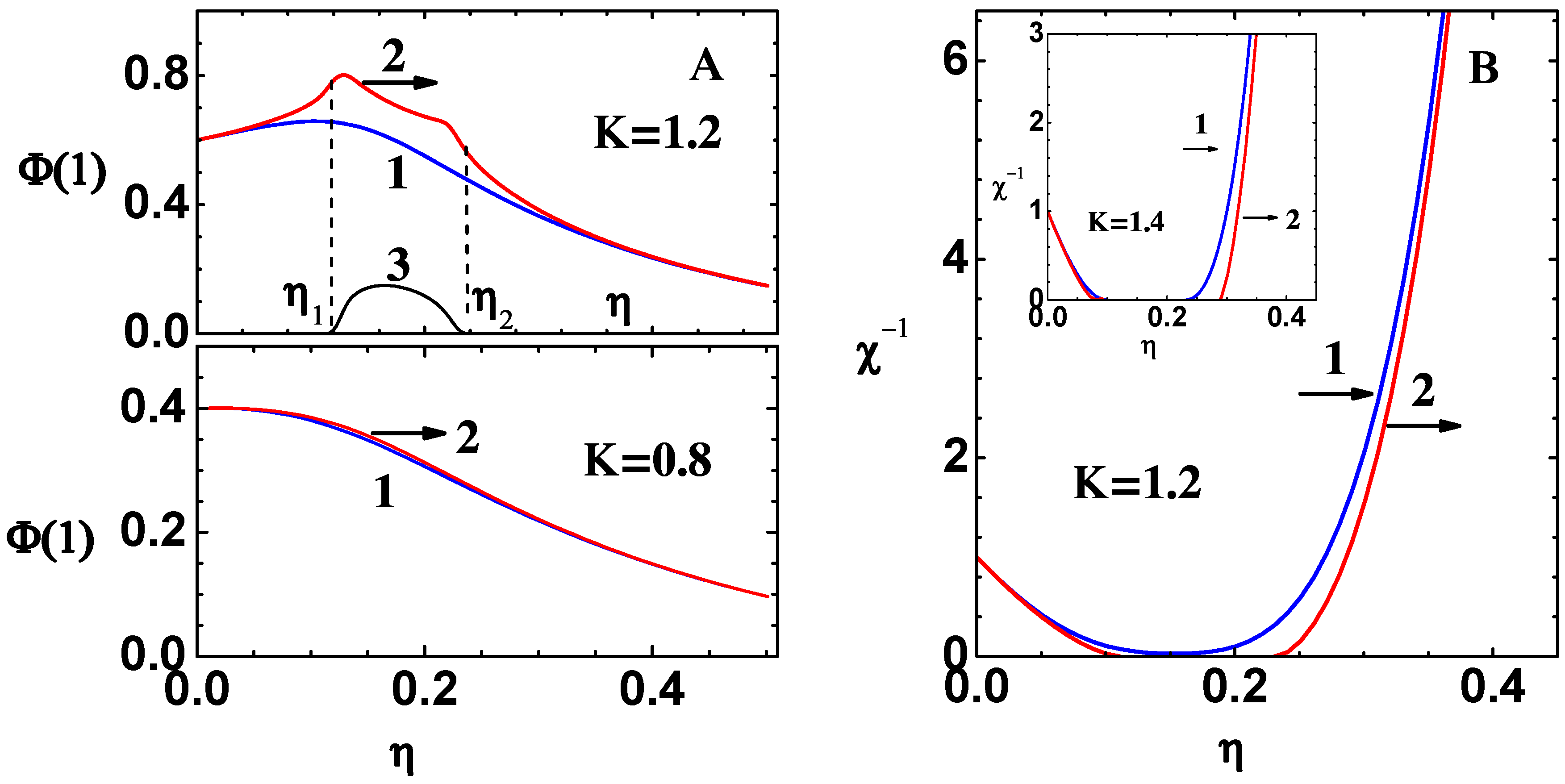
The series solution versus is compared with exact solutions, which are simply the roots of Equation (24), for two values of the parameter K in Figure 2A. These results are for the range parameter , which yields the critical value . The lower part (for ) shows , obtained from CPE of the 20th order (curve-1) and exact results (curve-2). The latter is the real root of Equation (24) discussed earlier. The two sets of results agree excellently, however, note that this case is in the region of K with two real solutions. The series solution converges quite fast, in fact, low order expansions (say 10th order) also yield similar comparisons. In the upper part of the figure (for ), the range is the ‘no-real-solution-region’. Graphs show , obtained from CPE of 20th order (curve-1), and real (curve-2) and imaginary (curve-3) parts of the exact root. Note that CPE does not yield the complex solutions, and there are also significant deviations outside the ‘no-real-solution-region’. However, data in Table 2 have demonstrated convergence of CPE in all regions; thus, the graph for in the upper part also corresponds to a convergent series. Exact results for (reduced) inverse compressibility (curve-2), obtained using analytical expressions [11], are compared in Figure 2B with those obtained by using CPE of 20th order (curve-1). The inset figure, which is for , shows that within CPE is non-negative in the entire range of . Note that exact values of are complex in the ‘no-real-solution-region’.
The results presented above for the AHS and MSA-HCY models show several features: (i) The CPE converges to exact results quite well in regions of phase plane where there are real solutions; (ii) the expansion fails to converge in ‘no-real-solution region’ of the AHS model, however, it converges even in that region for the MSA-HCY model; (iii) CPE is useful to derive the phase diagram by using thermodynamic conditions if it totally contains (as shown in the AHS model) the ‘no-real-solution region’.
5. Coupling Parameter Expansion—LJ Potential
This section presents numerical results for the more realistic LJ potential: , where and are, respectively, the depth and range parameters. The density-dependent bridge function given in Equation (5) defines the closure relation for OZE. This is important because the predictive power of OZE depends solely on the accuracy of the bridge function. In obtaining numerical results, CPE (outlined earlier) is truncated at the 7th order, i.e., expansion including terms up to are used throughout the analysis. Reduced temperature and density are the variables used, and the argument is omitted from different expressions.
The CPE around provides real solutions throughout the phase plane if the series expansion converges. In the case of AHS and MSA models, as discussed in previous sections, convergence is clearly evident above the gas-liquid phase transition temperature. However, for the more realistic model considered here, convergence can only be tested numerically at somewhat lower orders of expansions. The LJ model (and bridge function) is also analyzed by applying Newton’s method to the full potential [9], where provisions to search for complex solutions are also builtin. This analysis reveals features similar to those found in AHS model, i.e., occurrence of a ‘no-real-solution-line’ on the gaseous side of an isotherm below critical temperate. Compressiblility is found to be finite but complex along this line, but the constant-volume heat capacity diverges. Although there is no true spinodal line on the gaseous side, the same analysis has found one to the left of the co-existence line on the liquid side. The emergence of complex isothermal compressibility within the HNC closure is also presented as a ‘fold-bifurcation’ [29] on isotherms for sub-critical temperatures. In fact, this feature is observed with several other closures [30], including the one considered here. However, it appears that the HNC closure does not yield a true critical point because the isothermal compressibility is finite on both boundaries (on gaseous and liquid sides) of the ‘no-real-solution region’ [4,31]. However, the series expansion in CPE about the repulsive component of the potential will not pick up these complex solutions. Moreover, as shown below, CPE is useful for computing the phase diagram, either via the compressibility or the free energy routes. The latter does not require data corresponding to phase points in the spinodal region.
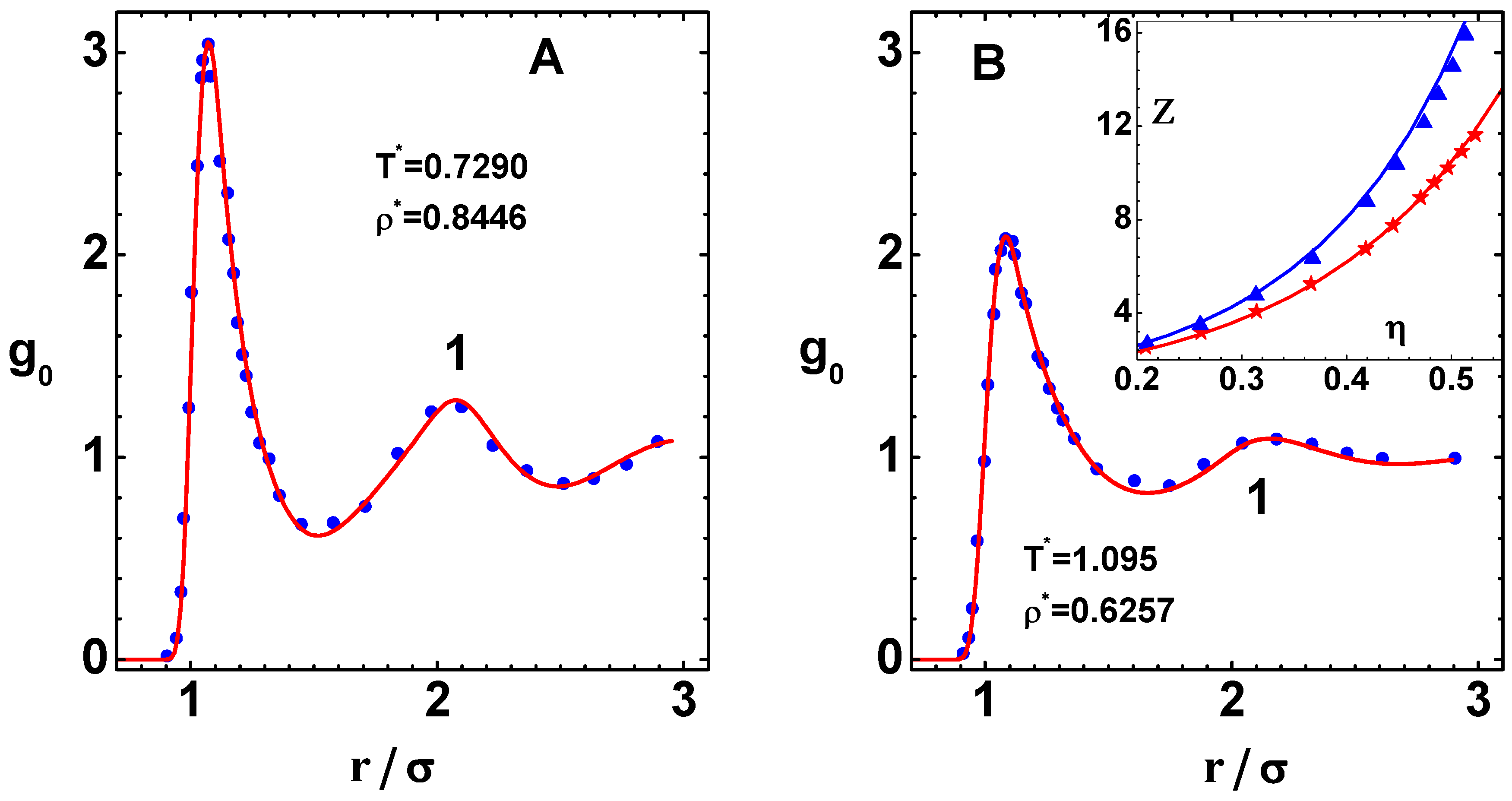
First of all, it is necessary to check the accuracy of modeling the reference system resulting from WCA prescription. To that end, the pair distribution function versus scaled distance (curve-1), which corresponds to and , is compared against molecular dynamics simulation data (symbols) [32] in Figure 3A. Similar comparisons are shown in Figure 3B for the case and . Excellent agreement found in peak heights and variations in the entire range of demonstrates the accuracy of the bridge function for the repulsive WCA potential. The compressibility factor versus the volume fraction, is compared against simulation data (symbols) [33] in the inset figure for two temperatures: (top curve) and (bottom curve). Here, the agreement is also quite good, although slight differences are noted at higher for the low temperature case. All these results, obtained via the compressibility route, are found to be superior than those from the virial route.
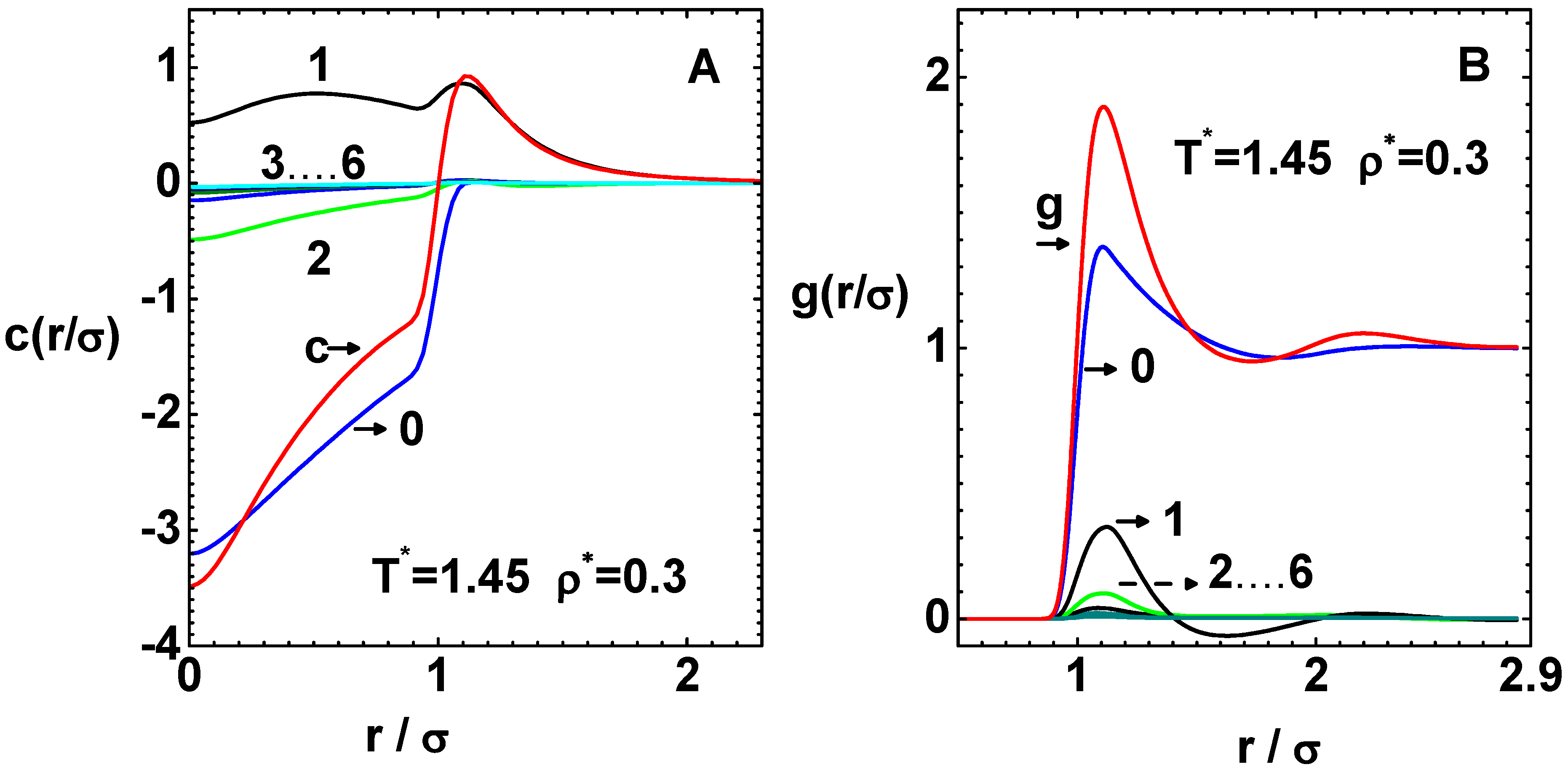
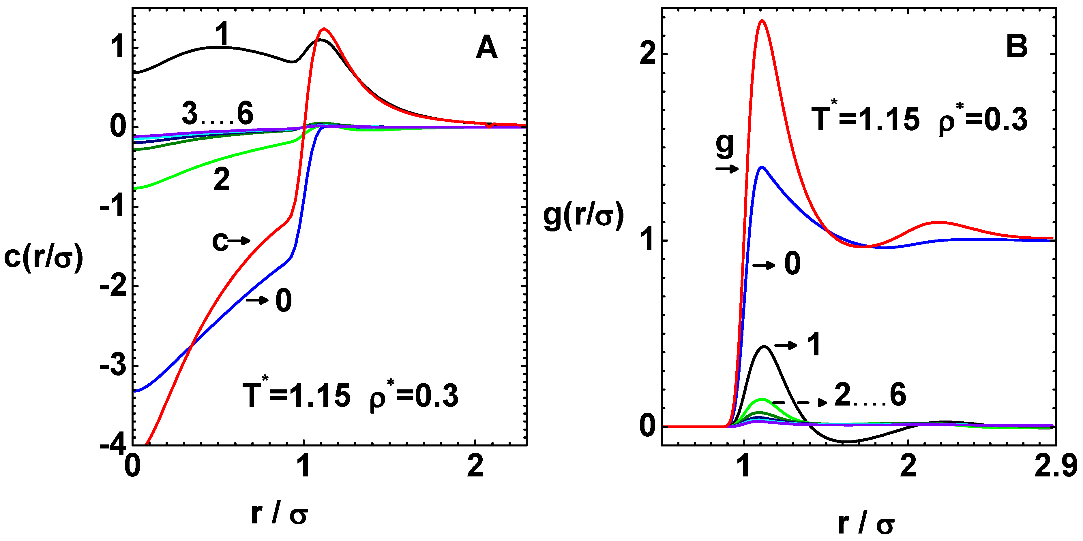
Next, the convergence of the correlation functions and is analyzed in Figure 4 for single phase region and Figure 5 for two phase region. The former figure corresponds to the phase point and , which is above the critical temperature, while the latter one is for and lying within the the spinodal region (see below). In both figures, the left and right panels (A and B) correspond to and , respectively. The functions (curve-c), the reference function (curve-0), and six successive derivative terms (curve-1 to curve-6) are shown in both left panels. Similarly, the two right panels show (curve-g), the reference function (curve-0), and six successive derivative terms (curve-1 to curve-6).
Convergence to well defined functions, shown as and , although based on numerical results, is evident at both phase points. Moreover, it is the first order term that contributes to the main correction. Note that the reference function is negative at both phase points; however, the graphs of for have positive parts, which arise due to attractive interactions. This positive component is more pronounced at the spinodal region (Figure 5A), and it leads to negative compressibility at that point (see below). The reference functions have only small first peaks at both phase points. However, the first and second peaks in are more pronounced in the spinodal region (Figure 5B). This is because of lower temperature at this point, which amplifies the effects of attractive interactions. These profiles of and in Figure 5 (for the sub-critical case) are similar to those corresponding to one of the real solutions in the spinodal region [10], although they are obtained with PY closure. This point is discussed in more detail in Section 5.3 below.
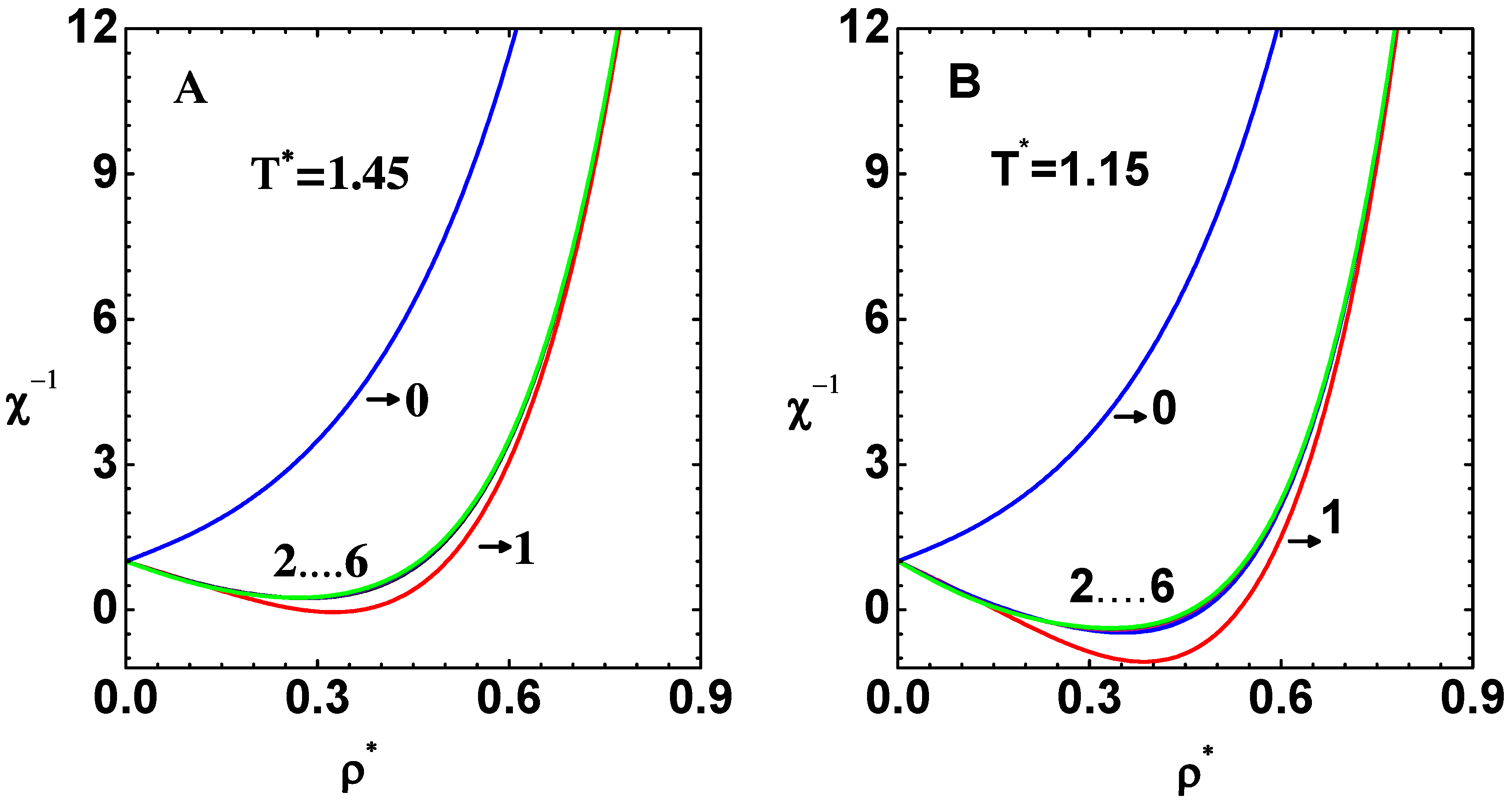
Graphs of inverse compressibility versus reduced density , obtained using Equation (14) at successive orders, are shown in Figure 6. Here, the left panel (A) is for (in one-phase region), while the right panel (B) corresponds to (in spinodal region). Note that the graphs depict partial sums of the series terms. Thus, were obtained using (curve-0), (curve-1), (curve-2), etc., and finally (curve-6) are shown in the panels. Similarly to the case of correlation functions, the main contribution of attractive potential comes up at first order corrections, although it over-corrects a bit. Both panels show convergence of the curves to well defined profiles of . It is positive in the entire range of for , as expected. However, for , there is a region of where is negative. Numerical values of for three values of , obtained with , are also given in Table 3. Data in column 3, for the case of and , are for a phase-point in the spinodal region. The sub-critical isotherms, obtained by integrating over density (starting from ), will show the familiar van der Waals loop due to the negative-value region. Thus, the thermodynamic properties obtained via CPE, although much more accurate, are similar to those of any first order mean field theory.
There is an issue related to the occurrence of negative compressibility (at any phase point) because it implies, by continuity requirements, that would vanish at some positive value . This is so because should tend to zero for sufficiently large k. Then, the transforms (see Equation (6)) and consequently would diverge at . Thus, negative compressibility at any phase point implies a singularity at a positive in the Fourier transform , which signals long ranged oscillations in the correlation function [9]. Truncated Taylor’s series employed in CPE will not yield this singular function. In fact, this function is the solution to OZE with the series approximation to . There is no inconsistency here, because it is known that OZE admits multiple solutions in the spinodal regions. As argued further in Section 5.3, only the series solution for obtained via CPE is relevant.
5.1. Phase Diagram of LJ Potential
Before obtaining the phase diagram, it is important to check the accuracy of CPE results on an isotherm close to the critical point. This is conducted in Figure 7A, which shows versus (curve-1) on isotherm for . The results of independent computations (symbols) are also shown [12]. The latter results are for identical models but are based on Newton’s method applied to the full potential, together with very careful strategies to mark out the spinodal region. The reduced temperature is just above the critical temperature and was obtained via CPE, as discussed next. The agreement between the two sets of results is quite good, thereby demonstrating convergence of profile in CPE even close to the critical point. The inset figure shows pressure (curve-1) and chemical potential (curve-2) obtained via the compressibility route, i.e., by integrating profile (see Equation (15)) from zero to . Nearly flat regions in these graphs over a range of show the closeness of the isotherm to the critical isotherm.
Next, the phase diagram (co-existence curves) of the LJ system obtained via CPE is compared against simulation data (symbols) [34]. Two schemes are used for this purpose: (i) thermodynamic conditions (i.e., and discussed earlier) via free energy route (curve-1) and (ii) Maxwell’s construction via compressibility route (curve-2). Note that the first scheme (see Equation (13)) is not dependent on the results within the spinodal region. The second scheme uses results in the negative compressibility region for obtaining P and its volume-integral on the liquid side of the phase-plane. The good agreement between the two schemes show that profiles in the spinodal region are accurate interpolations between those in the gas and liquid sides. There are only slight differences between the results of the two schemes, along the liquid branch near the transition point. The simulation data agree better with the results of the former. The critical point parameters are also obtained using two methods: (i) solving the defining equations, ; and (ii) extrapolating values of (over density) to zero on different isotherms in the one phase region. These methods provide almost identical critical point parameters: and , which compare well with simulation data given in square brackets. The spinodal lines on the gas and liquid sides (curve-3) are also shown in the figure.
The correlation functions and thermodynamic properties in the spinodal region, although converge to well defined profiles in CPE, are nonphysical, as they generate negative compressibility and van der Waals’s loop in pressure. However, their utility in computing the phase diagram (via thermodynamic conditions or Maxwell’s construction) is now demonstrated by comparing the results with those from independent methods. In any case, the weighted averaging of contributions of gas and liquid phases is needed to obtain physically acceptable properties.
5.2. Phase Diagrams of Generalized LJ(n,m) Potentials
The LJ potential is generalized to LJ() family of potentials, with arbitrary power law exponents n and m, in the following expression.
The pre-factor is chosen so that potential depth is for all n and m. Varying the exponent n, while keeping , generates a family of potentials, also called Mie (n,6) potentials. The effective potential-range is altered on varying n: A larger n yields arrow and smaller n broad potentials. These potentials have applications in modeling systems in soft matter physics and have been investigated via molecular dynamics simulations [35] and integral equation theory [12].
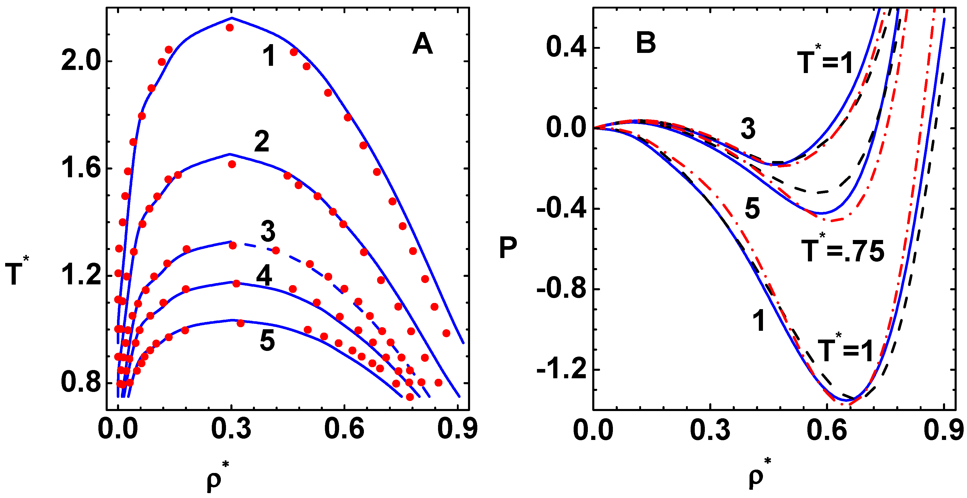
The phase diagrams, obtained with CPE, are compared with simulation data (symbols) [35] in Figure 8A for potentials LJ(7,6) (curve-1), LJ(9,6) (curve-2), LJ(12,6) (curve-3), LJ(15,6) (curve-4), and LJ(20,6) (curve-5). These results are obtained via the compressibility route mentioned earlier. Perhaps the results obtained via CPE offer better comparison with simulation data than that obtained using Newton’s method applied to full potential [12]. It is also possible in CPE to approach the critical point closer on both branches. The gaseous branches and critical points compare well for all cases. However, there are differences on the liquid side for , , and cases. In fact, CPE results lie above simulation data for softer cases (smaller n) where the trend is just opposite for harder (larger n) cases. Results agree quite well on both branches for intermediate values and . A possible reason for this is analyzed in Figure 8B, which shows the reduced isotherms for LJ(7,6) (curve-1) obtained via the virial (solid line), compressibility (dashed line), and free energy (dash-dot line) routes for . Similar sets of graphs for potentials LJ(12,6) (curve-3) at and LJ(20,6) (curve-5) at are also shown in the panel. These results indicate that the bridge function [22] provides much better thermodynamic consistency for the intermediate cases ( and 15) while important deviations are noted for softer and harder potentials. This might explain the differences in the phase diagrams on the liquid branch for the latter cases.
5.3. Solution-Spaces and Bifurcations of Solutions
The closure relation (Equation (4)) is solvable (in principle) so as to express in terms of explicitly. Then, OZE reduces to the following mapping: , where is a nonlinear operator. The specific details of will depend on the closure relation, bride function, and inter-particle potential. However, the important point is that the solutions to OZE are simply the fixed-points of the operator , acting on functions defined in a suitable metric space [36]. Stability of the fixed-points and bifurcation of solutions, resulting due to variation of parameters (such as and T) in , will crucially depend on the solution-space chosen for in addition to the specific properties of . If OZE is solved simply to obtain correlation functions, it is adequate to chose a solution-space , wherein functions tend to zero for sufficiently large values of r. However, it is necessary to impose the constraint , for employing to compute thermodynamic quantifies, as reduced compressibility (along an isotherm) is given by . The integral constraint, which ensures the existence of 3D Fourier transforms of functions (used for computing structure factor), restricts the solutions to a sub-space . Furthermore, numerical methods chosen to solve for the fixed-points, which are always of the iterative type, impose certain constraints on the solution so that iterations converge. It is common to modify the solution-algorithm, such as Newton’s method, and to look for complex solutions in regions where the method shows signs of diverging iterates [9].
The most efficient algorithms for solving OZE compute the convolution integral by using 3D Fourier transforms [6]. Baxter’s alternate formulation of OZE [8], applicable to cases where for (cutoff range), is defined entirely in . However, this formulation imposes the integral constraint mentioned above. The vanishing property of is exactly valid within PY closure when potential for , as in the AHS model. Both these approaches seek solutions in the sub-space ; algorithms used with them are also modified to detect bifurcations from real to complex solutions at some along a sub-critical isotherm [7,9]. The region between such values of in the gas and liquid sides on the isotherm is termed ‘no-solution-region’, as the original aim was only to find real solutions. More detailed bifurcation analysis that was mentioned earlier [29], using the pseudoarc-length continuation (PAL) algorithm, has provided the complete bifurcation curve (with HNC closure). The same algorithm (PAL), as well as the modified Newton’s method, has also yielded real solutions within this region at somewhat lower temperatures, although not continuously across the ‘no-solution-region’. A numerical treatment of the AHS model [37] has shown similar features, wherein two pairs of complex solutions and one real solution are detected.
The OZE given in Equation (3) may also be written in the radial coordinate () and solved numerically in a sufficiently long range , together with builtin asymptotic conditions (for ) [10]. These solutions would then belong to the less restricted space . Bifurcations of a real solution to three real solutions, along a sub-critical isotherm in the spinodal region, are found with this approach using PY closure [10]. Of the three solutions, two correspond to long ranged , which do not satisfy the integral constraint, and one to short ranged . Furthermore, the short ranged and corresponding yield negative compressibility along the part of the isotherm in the spinodal region. It is not known at present if this approach can also provide the complex solutions found in the sub-space .
The real series obtained via CPE for and, hence, (in the stable, metastable, and unstable regions), provides short ranged solutions because the linear integral operator in Equation (9) involves only the correlation functions of the reference system. Furthermore, the source terms in this equation, for all orders, result from functions obtained at lower orders. Since the method uses 3D Fourier transforms, CPE seeks solutions in the sub-space . The singular function , obtained by substituting the series for in Equation (6), would be a first approximation to one of the long ranged ; however, it lies outside the CPE method. This conclusion is based on the assumption that real solutions would be found in the spinodal region for the LJ model and closure used here, similarly to the PY case [10]. Finally, note that the closure relation rewritten as (see Equation (13)), together with the series for , can be used to obtain slightly improved results for pair correlation function.
6. Summary
The main aim in this paper is to analyze the convergence of CPE for solving the OZE. After providing brief details of CPE, its convergence is evaluated first for the two analytically solvable AHS and MSA models. Both these models show the emergence of a ‘no-real-solution-region’ in the two-phase domain of the phase plane. The CPE, which is based on series expansions around the correlation functions of the (repulsive) reference potential, always generate real solutions. Hence, it will not provide complex solutions to the OZE, obtained from several studies, in the two-phase region. The analytical arguments and numerical results presented for the AHS model show that CPE fails to converge in the ‘no-real-solution-region’. In fact, convergence is slow in the neighborhoods outside this region. However, this does not affect computation of the phase diagram of the AHS model because it completely contains the ‘no-real-solution-region’. Numerical results presented also show that CPE converges even in the ‘no-real-solution-region’ for the MSA-HCY model. The convergence issue is evaluated in detail for the LJ system modeled using an accurate density-dependent bridge function and 7th order solutions. Spatial profiles of correlation functions, corresponding to phase points above as well as below the critical point, are found to approach well defined functions. Similarly, density-profiles of inverse compressibility (above, below, and close to critical point) also converge toward appropriate functions. The phase diagrams of LJ model obtained via two schemes, one using the free energy and the other using the compressibilty routes, agree well and also with simulation data. The two schemes are independent as the free energy route uses only results corresponding to phase points outside the spinodal region. It is argued that CPE provides proper real solutions to OZE in the stable, metastable, and spinodal region. The whole procedure is also evaluated with reference to simulation data on the generalized LJ(n,6) family of potentials. These potentials with variable ranges have important applications in soft condensed matter. The main conclusion of this paper is that CPE provides a practical approach to evaluate the thermodynamic proprieties of one of the component fluids described by using general pair-potentials.
Funding
This research received no external funding.
Institutional Review Board Statement
Not applicable.
Informed Consent Statement
Not applicable.
Data Availability Statement
Not applicable.
Acknowledgments
The author thanks the three reviewers of for critical reviews and suggestions to improve the presentation of the paper.
Conflicts of Interest
The author declares no conflict of interest.
References
- Hansen, J.P.; McDonald, I.R. Theory of Simple Liquids, 4th ed.; Academic Press: Cambridge, UK, 2013. [Google Scholar]
- Martynov, G.A. The problem of phase transitions in statistical mechanics. Physics-Uspekhi 1999, 42, 517. [Google Scholar] [CrossRef]
- Sarkisov, G.N. Approximate equations of the theory of liquids in the statistical thermodynamics of classical liquid systems. Physics-Uspekhi 1999, 42, 545. [Google Scholar] [CrossRef]
- Caccamo, C. Integral equation theory description of phase equilibria in classical fluids. Phys. Rep. 1996, 274, 1–105. [Google Scholar] [CrossRef]
- Kelley, C.T. Solving Nonlinear Equations with Newton’s Method; Fundamentals of Algorithms; SIAM: Philadelphia, PA, USA, 2003. [Google Scholar]
- Zerah, G. An efficient Newton’s method for numerical solution of fluid integral equations. J. Comp. Phys. 1985, 61, 280. [Google Scholar] [CrossRef]
- Watts, R.O. Percus-Yevick equation applied to a Lennard-Jones fluid. J. Chem. Phys. 1968, 48, 50. [Google Scholar] [CrossRef]
- Baxter, R.O. Percus-Yevick equation of hard spheres with surface adhesion. J. Chem. Phys. 1968, 49, 2770. [Google Scholar] [CrossRef]
- Sarkisov, G.N.; Lomba, E. The gas-liquid phase transition singularities in the framework of the liquid-state integral equation formalism. J. Chem. Phys. 2005, 122, 214504. [Google Scholar] [CrossRef] [Green Version]
- Mier y Teran, L.; Falls, A.H.; Scriven, L.E.; Davis, H.T. Structure and thermodynamics of stable, metastable, and unstable fluid—Efficient numerical method for solving the equations of equilibrium fluid physics. Proc. Eighth Symp. Thermophys. Prop. 1982, 8, 45. [Google Scholar]
- Cummings, P.T.; Smith, E.R. Liquid-gas transition for hard spheres with attractive Yukawa tail interactions. Chem. Phys. 1979, 42, 341. [Google Scholar] [CrossRef]
- Charpentier, I.; Jakse, N. Phase diagram of complex fluids using an efficient integral equation method. J. Chem. Phys. 2005, 123, 204910. [Google Scholar] [CrossRef] [PubMed]
- Solana, J.R. Perturbation Theories for Thermodynamic Properties of Fluids and Solids; CRC Press: New York, NY, USA, 2013. [Google Scholar]
- Zhou, S.; Solana, J.R. Progress in the perturbation approach in fluid and fluid-related theories. Chem. Rev. 2009, 109, 2829. [Google Scholar] [CrossRef]
- Tang, Y.; Lu, B.C.Y. A new solution of the Ornstein-Zernike equation from perturbation theory. J. Chem. Phys. 1993, 99, 9828. [Google Scholar] [CrossRef]
- Sai Venkata Ramana, A.; Menon, S.V.G. Coupling-parameter expansion in thermodynamic perturbation theory. Phys. Rev. 2013, E87, 022101. [Google Scholar]
- Weeks, J.D.; Chandler, D.; Andersen, H.C. Role of Repulsive Forces in Determining the Equilibrium Structure of Simple Liquids. J. Chem. Phys. 1971, 54, 5237. [Google Scholar] [CrossRef]
- Menon, S.V.G. Scaling of phase diagram and critical point parameters in liquid-vapor phase transition of metallic fluids. Condens. Matter 2021, 6, 6. [Google Scholar] [CrossRef]
- Levashov, P.R.; Fortov, V.E.; Khishchenko, K.V.; Lomonosov, I.V. Equation of state for liquid metals. AIP Conf. Proc. 2000, 505, 89. [Google Scholar]
- Levashov, P.R.; Fortov, V.E.; Khishchenko, K.V.; Lomonosov, I.V. Analysis of isobaric expansion data based on soft-sphere equation of state for liquid metals. AIP Conf. Proc. 2002, 620, 71. [Google Scholar]
- Menon, S.V.G.; Nayak, B. An equation of state for metals at high temperature and pressure in compressed and expanded volume regions. Condens. Matter 2019, 4, 71. [Google Scholar] [CrossRef] [Green Version]
- Sarkisov, G.N. Structure of simple fluid in the vicinity of the critical point: Approximate integral equation theory of liquids. J. Chem. Phys. 2003, 119, 373. [Google Scholar] [CrossRef]
- Kelley, C.T.; Pettitt, B.M. A fast solver for Ornstein-Zernike equations. J. Comp. Phys. 2004, 197, 491. [Google Scholar] [CrossRef] [Green Version]
- Lado, F. Perturbation correction for the free energy and structure of simple fluids. Phys. Rev. 1973, A8, 2548. [Google Scholar] [CrossRef] [Green Version]
- Barboy, B. On a representation of the equation of state of fluids in terms of the adhesive hard-sphere model. J. Chem. Phys. 1974, 61, 3194. [Google Scholar] [CrossRef]
- Baxter, R.J. Ornstein-Zernike relation for a disordered fluid. Aust. J. Phys. 1968, 21, 563. [Google Scholar] [CrossRef] [Green Version]
- Menon, S.V.G.; Manohar, C.; Srinivasa Rao, K. A new interpretation of the sticky hard sphere model. J. Chem. Phys. 1991, 95, 9188. [Google Scholar] [CrossRef]
- Waisman, E. The radial distribution function for a fluid of hard spheres at high densities Mean spherical integral equation approach. Mol. Phys. 1973, 25, 45. [Google Scholar] [CrossRef]
- Peplow, A.T.; Beardmore, R.E.; Bresme, F. Algorithms for the computation of solutions of Ornstein-Zernike Equation. Phys. Rev. 2006, E74, 046705. [Google Scholar] [CrossRef] [PubMed]
- Tikhonov, D.A.; Sarkisov, G.N. Singularities of solution of the Ornstein-Zernike Equation within the gas-liquid transition region. Russ. J. Phys. Chem. 2000, 74, 470. [Google Scholar]
- Brey, J.J.; Santos, A. Absence of criticality in hypernetted chain equation for a truncated potential. Mol. Phys. 1986, 57, 149. [Google Scholar] [CrossRef]
- Gubbins, K.E.; Smith, W.R.; Tham, M.K.; Tiepel, E.W. Perturbation theory for the radial distribution function. Mol. Phys. 1971, 22, 1089. [Google Scholar] [CrossRef]
- Heyes, D.M.; Okumura, H. Equation of state and structural properties of Weeks-Chandler-Andersen fluid. J. Chem. Phys. 2006, 124, 164507. [Google Scholar] [CrossRef]
- Johnson, J.K.; Zollweg, J.A.; Gubbins, K.E. The Lennard-Jones equation of state revisited. Mol. Phys. 1993, 78, 591. [Google Scholar] [CrossRef]
- Okumura, H.; Yonezawa, F. Liquid–vapor coexistence curves of several inter-atomic model potentials. J. Chem. Phys. 2000, 113, 9162. [Google Scholar] [CrossRef]
- Malescio, G.; Giaquinta, P.V.; Rosenfeld, Y. Iterative solutions of integral equations and structural stability of fluids. Phys. Rev. 1998, E57, R-3723. [Google Scholar] [CrossRef]
- Monson, P.A.; Cummings, P.T. Solution of the Percus-Yevick equation in the coexistence region of a simple fluid. Int. J. Thermo. Phys. 1985, 6, 573. [Google Scholar] [CrossRef]
Figure 1.
(A) Upper part shows versus from CPE of 20th order for (curve-1), (curve-2), and exact results (symbols). The range is the ‘no-real-solution-region’ for . Lower part of the figure for shows compressibility pressure P versus , from CPE of 20th order (curve-1), and exact results (symbols). The blank portion is the ‘no-real-solution-region’. (B) The exact results for phase diagram of AHS model (blue line and symbols) are compared with those obtained using a CPE of 50th order (curve-2) and 20th order (curve-3). The ‘no-real-solution-region’, lying within the dashed lines (curve-1), is also shown.

Figure 2.
(A) Lower part (for shows versus obtained from CPE of 20th order (curve-1) and the exact results (curve-2). In the upper part (for , the range is ‘no-real-solution-region’, as . Graphs show versus obtained from CPE of 20th order (curve-1) and real (curve-2) and imaginary (curve-3) parts of the exact results. (B) Graphs show (reduced) inverse compressibility versus obtained from CPE (curve-1) and exact results [11] (curve-2) for . The inset figure is similar, but it is for .

Figure 3.
(A) Pair distribution function versus scaled distance (curve-1) for the reference system of LJ potential, as per the WCA prescription (see text), at reduced temperature and density . Symbols are molecular dynamics simulation results [32]. (B) Similar results for the parameters and density . The inset figure shows compressibility factor versus volume fraction for reduced temperature (top curve) and (bottom curve). Symbols are simulation results [33].

Figure 4.
Convergence of direct correlation function and pair distribution function for the LJ system at the phase point and , which is above the critical temperature. (A) Graphs show (curve-c), reference function (curve-0), and successive derivative terms (curve-1 to curve-6). (B) Similarly, the graphs show (curve-g), reference function (curve-0), and derivative terms (curve-1 to curve-6) for the same phase point.

Figure 5.
Convergence of direct correlation function and pair distribution function for the LJ system at the phase point and , which is in the spinodal region. (A) Graphs show (curve-c), reference function (curve-0), and successive derivative terms (curve-1 to curve-6). (B) Similarly, the graphs show (curve-g), reference function (curve-0), and derivative terms (curve-1 to curve-6) for the same phase point.

Figure 6.
Graphs show inverse compressibility versus reduced density obtained at successive orders of series expansion. Thus, calculated with just (curve-0), (curve-1), (curve-2), etc., and finally (curve-6) is shown. (A) Graphs for reduced temperature in one-phase region. (B) Similarly, for when crossing the spinodal region.

Figure 7.
(A) Comparison of versus obtained by using CPE (curve-1) and independent computations (symbols) [12] on the isotherm for , which is just above the critical temperature. The inset graphs show pressure (curve-1) and chemical potential (curve-2) (both obtained via compressibility route) on the same isotherm. (B) Comparison of co-existence lines using thermodynamic conditions (curve-1) and Maxwell’s construction (curve-2) with the simulation results (symbols) [34], obtained with CPE. The spinodal lines (curve-3) on gaseous and liquid sides are also shown.

Figure 8.
(A) Comparison of co-existence lines, obtained with CPE, for potentials: LJ(7,6) (curve-1), LJ(9,6) (curve-2), LJ(12,6) (curve-3), LJ(15,6) (curve-4), and LJ(20,6) (curve-5), with simulation data (symbols) [35]. (B) Reduced isotherms for LJ(7,6) (curve-1) using virial (solid line), compressibility (dashed line), and free energy (dash-dot line) routes corresponding to . Other sets of graphs are for LJ(12,6) (curve-3) at and LJ(20,6) (curve-5) at .


Table 1.
Convergence of CPE coefficients in AHS model.
| AHS Model | = 0.45 | ||
|---|---|---|---|
| n | = 0.05 | = 0.15 | = 0.25 |
| 1 | 2.11588 | 1.90467 | 1.69443 |
| 6 | 0.769139 | 1.93929 | 3.16261 |
| 11 | 0.823916 | 1.00009 | 0.764407 |
| 16 | 0.881579 | 0.948853 | 0.716068 |
| 21 | 0.90604 | 0.959392 | 0.842613 |
| 26 | 0.918982 | 0.971881 | 0.878875 |
| 31 | 0.927508 | 0.981006 | 0.880897 |
| 36 | 0.933696 | 0.987649 | 0.884413 |
| 41 | 0.938408 | 0.992688 | 0.889093 |
| 46 | 0.942117 | 0.996646 | 0.892829 |
| 51 | 0.945112 | 0.999839 | 0.895698 |
Table 2.
Convergence of CPE coefficients in the MSA-HCY model.
| MSA-HCY Model | K = 1.2 | ||
|---|---|---|---|
| n | |||
| 2 | 0.203451 | 0.233279 | 0.187291 |
| 6 | 0.568111 | 0.612217 | 0.454637 |
| 11 | 0.648161 | 0.689816 | 0.499086 |
| 16 | 0.678529 | 0.719187 | 0.51365 |
| 21 | 0.694581 | 0.734819 | 0.520534 |
| 26 | 0.704522 | 0.744575 | 0.524387 |
| 31 | 0.711287 | 0.751261 | 0.526771 |
| 36 | 0.71619 | 0.756136 | 0.528354 |
| 41 | 0.719906 | 0.75985 | 0.529465 |
| 46 | 0.722821 | 0.762777 | 0.53029 |
| 51 | 0.725169 | 0.765143 | 0.530938 |
Table 3.
Partial sums of LJ model inverse compressibility series in CPE.
| Order | Inverse Compressibility | Inverse Compressibility | ||||
|---|---|---|---|---|---|---|
| 1 | 1.47757 | 4.53543 | 13.6363 | 1.46285 | 4.35925 | 12.6832 |
| 2 | 0.434523 | −1.13238 | 2.19019 | 0.632217 | −0.091533 | 3.77993 |
| 3 | 0.396093 | −0.532527 | 2.79679 | 0.606776 | 0.283586 | 4.16096 |
| 4 | 0.369497 | −0.491079 | 2.85451 | 0.592575 | 0.304848 | 4.19282 |
| 5 | 0.352317 | −0.459612 | 2.88001 | 0.585209 | 0.318156 | 4.20459 |
| 6 | 0.342099 | −0.43545 | 2.89254 | 0.581667 | 0.326561 | 4.20943 |
| 7 | 0.335684 | −0.416063 | 2.89917 | 0.579865 | 0.332105 | 4.21159 |
Publisher’s Note: MDPI stays neutral with regard to jurisdictional claims in published maps and institutional affiliations. |
© 2021 by the author. Licensee MDPI, Basel, Switzerland. This article is an open access article distributed under the terms and conditions of the Creative Commons Attribution (CC BY) license (https://creativecommons.org/licenses/by/4.0/).
Share and Cite
MDPI and ACS Style
Menon, S.V.G. Convergence of Coupling-Parameter Expansion-Based Solutions to Ornstein–Zernike Equation in Liquid State Theory. Condens. Matter 2021, 6, 29. https://doi.org/10.3390/condmat6030029
AMA Style
Menon SVG. Convergence of Coupling-Parameter Expansion-Based Solutions to Ornstein–Zernike Equation in Liquid State Theory. Condensed Matter. 2021; 6(3):29. https://doi.org/10.3390/condmat6030029
Chicago/Turabian StyleMenon, S. V. G. 2021. "Convergence of Coupling-Parameter Expansion-Based Solutions to Ornstein–Zernike Equation in Liquid State Theory" Condensed Matter 6, no. 3: 29. https://doi.org/10.3390/condmat6030029