
Opportunistic Strategy for Maintenance Interventions Planning: A Case Study in a Wastewater Treatment Plant


Department of Industrial Engineering, Universidad Técnica Federico Santa María, España Av. 1680, Valparaíso 2340000, Chile
*
Author to whom correspondence should be addressed.
Appl. Sci. 2021, 11(22), 10853; https://doi.org/10.3390/app112210853
Submission received: 27 September 2021
/
Revised: 28 October 2021
/
Accepted: 9 November 2021
/
Published: 17 November 2021
(This article belongs to the Special Issue Anaerobic Digestion Processes for Wastewater Treatment)
Abstract
:Featured Application
The application potential includes any sewage treatment system that makes use of preventive maintenance plans for highly critical assets, and requires the utilization of an optimized grouping strategy to improve the availability of the components involved.
Abstract
Wastewater treatment plants (WWTPs) face two fundamental challenges: on the one hand, they must ensure an efficient application of preventive maintenance plans for their survival under competitive environments; and on the other hand, they must simultaneously comply with the requirements of reliability, maintainability, and safety of their operations, ensuring environmental care and the quality of their effluents for human consumption. In this sense, this article seeks to propose a cost-efficient alternative for the execution of preventive maintenance (PM) plans through the formulation and optimization of the opportunistic grouping strategy with time-window tolerances and non-negligible execution times. The proposed framework is applied to a PM plan for critical high-risk activities, addressing primary treatment and anaerobic sludge treatment process in a wastewater treatment plant. Results show a 26% system inefficiency reduction versus the initial maintenance plan, demonstrating the capacity of the framework to increase the availability of the assets and reduce maintenance interruptions of the WWTP under analysis.
1. Introduction
1.1. The Relevance of Modern Maintenance Management in WWTPs
As technological development and operational efficiency increase within organizations, the production systems reveal a continuous increase of their complexity levels, while simultaneously consumers, stakeholders, and communities demand higher quality, reliability, and sustainability of the products and services required [1]. The interaction of these phenomena has generated radical changes within organizations, mainly in the way of meeting the demands of the interested parties, orienting themselves toward a holistic and multidisciplinary approach [2]. In this scenario, modern maintenance management has changed from being considered an auxiliary discipline necessary to maintain the operational status of equipment and assets, to becoming an essential strategic business function in many industries, not only for improving the reliability and productivity levels of the production systems involved, but also to increase the profitability of operations [3,4,5].
In the maintenance management context, the utilization of optimization tools during the maintenance planning stage can offer substantial savings regarding Operation and Maintenance (O&M) costs, considering that the potential for cost reduction can reach between 10 and 20% of the maintenance budget, and the latter can even exceed total operational costs in several industries [4,6]. On the other hand, optimized planning of maintenance activities in organizations can offer substantial improvements in the availability and productivity levels of the systems involved [6]; hence the need to devote a considerable effort for the generation of cost-effective, flexible, and fast-deployable maintenance plans, offering wide applicability and adaptability to different industrial settings and environments [3,7].
In the case of the wastewater treatment process, the industry needs to optimize the use of resources to achieve the expected service levels, which necessarily implies the use of efficient management strategies within treatment plants to ensure their survival under competitive industrial environments [8]. At the same time, water quality standards are becoming more and more stringent to prevent the negative impact of wastewater discharges on the environment [9]. Furthermore, this industry faces an additional challenge: service failures and breakdowns do not only establish an operational cost increase, but also represent a potential risk of environmental damage due to its malfunction [8]. Therefore, wastewater treatment plants (WWTPs) must constantly develop efficient managerial strategies, not only in the management of their operational resources and in the application of maintenance plans and policies, but also in the proper management of wastewater, ensuring the quality of service and environmental management of water resources [10,11].
1.2. Wastewater Treatment Plants and the Need for Cost-Effective Preventive Maintenance Strategies
Wastewater treatment is essential to protect human health and ensure the environmental sustainability of the planet [8]. Besides the relevance of stabilization and treatment of effluents for human consumption, wastewater treatment-related processes represent a fundamental task in a wide variety of industries such as livestock, chemical, and mining [12]. In response to the industrial and government requirements and protocols, wastewater treatment can be carried out through a wide variety of physical, chemical, and biological processes [13]. In this regard, biological processes, including anaerobic digestion processes, have demonstrated economic advantages over other treatment processes in terms of invested capital and related operational costs [12].
Biosolids that are generated from the primary and secondary wastewater treatment processes are denominated sludge. Generally, municipal sludge contains a wide variety of organic and inorganic materials, including biomass, oils, heavy metals, synthetic materials, and pathogens; for this reason, these solids must be necessarily pretreated before their disposal [13]. Within the wastewater treatment process, the treatment and use of sewage sludge have become an international waste management problem. In this sense, the digestion process in sludge treatment has become the first step in the reuse chain, representing up to 50% of the operational costs in sewage treatment plants [13,14]. Additionally, the sewage treatment process establishes a valuable source of raw materials, especially for obtaining nutrients, energy, and water for human consumption [9].
Within the municipal sludge treatment systems, anaerobic digestion processes have demonstrated wide application and positive externalities as a sustainable technology [15,16]. Anaerobic digestion consists of a series of biological processes in which several microorganisms decompose biodegradable materials in the absence of oxygen, differing in this regard from aerobic treatment systems such as, e.g., activated sludge processes [13,17]. During the anaerobic digestion process, microorganisms convert the organic material into mainly two products: digestate and biogas. The latter is mainly composed of carbon dioxide and methane, which can be used to generate electricity and heat, starting from the decomposition of biodegradable organic materials [18]. By the implementation of digestion processes, the formation of odors is eliminated and pathogens are destroyed, also generating a stabilization of the organic product [19]. For these reasons, anaerobic digestion processes have received increasing attention in several countries and organizations during the past decades [17].
Anaerobic digesters or anaerobic reactors can be used both for sewage pretreatment and sludge stabilization. Upflow anaerobic sludge reactors (UASB) closely resemble those for sewage treatment, except that: (a) Recirculation of the sludge and its mechanical agitation are kept to a minimum or omitted; (b) the reactor is equipped in the upper part with a system for separation of solid-gas phases [20]. This type of digester has been successfully implemented in recent years for the treatment of municipal wastewater, achieving high efficiency in the removal of suspended solids and biodegradable organic matter in countries with warmer climates [21]. In addition, sludge from high-strength wastewaters, for example, are preferably treated by anaerobic processes, thus providing potential for energy generation while producing low-surplus sludge [12].
Although anaerobic digestion processes, in general, have demonstrated a compact design and positive performance, they have evidenced certain difficulties, e.g., in providing complete stabilization in the case of high resistance water treatment. For this reason, several alternatives have been proposed to provide a cost-effective and efficient treatment for the management of sewage sludge, such as, for example, hybrid systems which combine anaerobic and aerobic processes simultaneously [12]. Alternatively, wastewater treatment plants must respond to an effective and efficient application of their maintenance plans, especially on preventive maintenance (PM) activities, considering the environmental impact that an operational malfunction may eventually cause. In this sense, several studies confirm that the lack of optimal PM plans in industries tends to increase the costs of repairable assets, deteriorating the productivity levels, and entailing social and environmental risks [22,23,24].
As in many reported industrial cases, sewage treatment plants have the potential to improve cost-efficiency through an optimized strategy for the execution of PM plans, considering that WWTP maintenance costs may represent 25% of total operational costs [8]. Additionally, the maintenance plans designed for complex systems address a wide variety of maintenance activities, each with its specifications, execution periods, and technical requirements. In this context, the application of PM activity grouping strategies can be particularly useful, representing a cost-efficient solution for multi-component production systems with high economic dependence, and where the costs associated with scheduled and non-scheduled system stoppages (i.e., system inefficiency costs) are significantly higher than the individual execution costs of the maintenance plan (i.e., direct execution costs).
1.3. Maintenance Grouping Strategies and Literature Review
In the maintenance planning context, the grouping strategy establishes a time span over which a joint execution of a certain number of maintenance activities is planned (See e.g., [25,26]). Through the application of the grouping strategy, it is possible to reduce the system setup costs related to the preparation, assembly, or disassembly of components when performing maintenance tasks. In the case of multi-component series systems, the grouping strategy also allows increasing system availability and consequently improving efficiency and productivity levels, while reducing the number of interruptions and downtime service [27]. In this regard, the scientific literature shows a wide application of this type of strategy in several industries, addressing the technical features of the productive environments, as well as the complexity and interaction between its components. In this sense, Thomas [28] originally proposed three types of multi-component system dependencies, namely: economic, structural, and stochastic. In this way, it is possible to classify the strategies proposed in the scientific literature, depending on the interactions addressed in each particular case.
The economic dependence on a production system establishes that the joint execution of maintenance activities is economically more efficient than their individual executions. In this way, the grouping strategy then implies a reduction in total maintenance costs. The vast majority of research related to the application of these strategies seeks to exploit this phenomenon in economic-dependent systems (see Hameed and Vatn [29], Zhou et al. [30], Xia et al. [31], Van et al. [32], Do et al. [26], Pandey et al. [33], Zhu et al. [34], Wu et al. [35], Zhou and Yu [36]). Addressing economic dependency, Mena et al. [34] develops a framework for planning PM activities, considering the use of time-window tolerances for the advance or delay in the execution of activities under a controlled risk zone, facilitating the creation of grouping schemes in a continuous-time planning horizon. Considering the close strategic relationship between operational and maintenance functions, recent research extends the grouping problem from a joint optimization approach to operational and maintenance management (See e.g., Nourelfath and Châtelet [37], Xiao et al. [38], Bertolini et al. [39], Zhou and Shi [40], Chen et al. [41]).
In several production systems, scientific literature in the field have shown the presence of different types of interactions or dependencies, which cannot be omitted when developing and implementing an efficient grouping strategy. For this reason, recent research in the field addresses several dependency types in complex systems. Structural dependence, on the one hand, includes the requirements for replacement, repair, and assembly of other work units to carry out the maintenance activity on a certain component [28]. In this sense, Dao and Zuo [42] address the existence of structural dependence for the evaluation of a selective grouping and maintenance strategy in multi-state multi-component series systems. On the other hand, stochastic dependence establishes the existence of lifetime correlation and deterioration between the different components of the production system. Recently, the research developed in Vijayan and Chaturbedi [43] simultaneously addresses the economic and stochastic dependence in multi-component systems, while research works such as Lu and Zhou [44], and Fan et al. [45] address the stochastic dependence phenomenon by modeling the deterioration of the components.
In the context of sewage treatment plants, some studies have addressed the impact of maintenance and renewal policies on the performance and efficiency of the plants, revealing a strong relationship between the management and application of said policies, the proportion of O&M costs, and the productivity levels. Hernández-Chover et al. [8] assess the effect of maintenance strategies on the efficiency of the facilities for a sample of WWTPs, establishing a correlation analysis between the non-parametric efficiency indicator data envelopment analysis (DEA) and the maintenance cost items. The results show that higher investment in preventive maintenance offers not only a reduction in total repair costs, but also a positive effect on overall efficiency indicators. Similarly, Ozgun et al. [9] propose the determination and analysis of cost functions in several full-scale sewage treatment plants, disaggregating capital costs (investment and equipment), and O&M costs on a sample of facilities in Istanbul. The study establishes, corroborating the results of previous studies, that higher treatment levels increase O&M costs, especially in tertiary treatment plants, reaching 58% of the total costs. This fact could be partly explained by the number and complexity of the components required for tertiary treatment. Additionally, O&M costs are fundamentally composed of energy supply costs and labor costs, reaching 39% and 31% of the total costs in tertiary treatment plants, respectively. These research works reveal the relevance of both energy cogeneration and the implementation of maintenance strategies to improve the cost-efficiency of wastewater treatment facilities.
1.4. Research Contribution
Despite the extensive amount of research in the field, to the best of our knowledge, there is no evidence of case studies observed for the application and implementation of preventive maintenance grouping strategies in sewage treatment plants. However, recent studies reveal a positive impact on the application of maintenance policies in the industry, establishing a high correlation between investment in preventive maintenance, savings in energy consumption, and increases in global efficiency indexes [8]. In this way, the research gap reveals two fundamental aspects that this study seeks to exploit: (1) The absence of case studies that address the application of maintenance grouping strategies in the water treatment industry; (2) and besides, the need for adaptive, flexible, and fast implementation strategies of PM plans in the wastewater facilities in response to efficiency, productivity, and quality of service requirements. In summary, this research proposes a new strategy to improve cost-efficiency and asset availability in wastewater treatment plants, with a focus on the implementation of the grouping framework during the maintenance planning and scheduling stages.
The framework presented below considers the extension of the formulation originally presented in Mena et al. [46], addressing the application of new criteria to improve the applicability and adherence of the strategy in industrial environments, through the incorporation of time-window tolerances for the creation of opportunistic grouping schemes and non-negligible PM execution times. Following the research line, the framework proposed in this article seeks to improve the availability level of complex production systems, reducing the number of system interruptions, while minimizing maintenance costs through the distribution of stoppage costs for PM activities.
The article is structured as follows: Section 2 presents the established Methodology for the application of the opportunistic grouping strategy; Section 3 presents the results obtained under the application of the strategy; Section 4 discusses the results and their impact on the analyzed case study; Section 5 establishes recommendations, limitations, and future research in the field.
Research gaps found in the literature:
- Absence of case studies addressing formulation and implementation of maintenance grouping strategies in the wastewater treatment industry;
- New and tailored strategies for an adaptive, flexible, and fast implementation of PM plans in the wastewater facilities, seeking to improve cost-efficiency and quality requirements.
Main contributions of the study:
- Presentation of a novel case study for the implementation of preventive maintenance execution strategy in wastewater and sludge treatment facilities;
- Framework formulation and computational optimization of a grouping strategy for preventive maintenance activities, seeking to minimize the number of planned interruptions, fixed maintenance costs, and system downtime;
- Adaptation of the grouping strategy to the case study under analysis, in response to the requirements of maintenance cost reduction, productivity, and quality of service required on wastewater facilities;
- In-depth discussion of results and recommendations with a focus on managerial insights.
2. Materials and Methods
The research methodology addresses five essential aspects: the presentation and context of the sludge and wastewater treatment process in the case study; the formulation of the optimization model for the opportunistic strategy; computational implementation and programming settings; and the discussion of the proposed performance indicators.
2.1. Wastewater Treatment Process: Case Study
The research addresses the study of the primary and sludge treatment in a WWTP for human consumption. The first stage considers a preliminary treatment, which consists of the removal of coarse fine solids, and sand. The preliminary treatment is followed by the sedimentation process, removing approximately 40% of biochemical oxygen demand (BOD) and 50% total suspended solids (TSS). After the primary treatment by flocculation and settling process, the water effluent continues its course to the secondary treatment. At the same time, the WWTP also considers the biologic treatment of sludge generated from the lamellar settling stage, going through an anaerobic digestion process, until its final disposal in a storage silo to become a sanitary landfill. The primary wastewater treatment process is set up from the stages described in Figure 1.
In the WWTP understudy, it is possible to consider three fundamental processing lines: wastewater, biogas, and sludge treatment. The sludge is produced as waste from the primary treatment phase and is transformed to treated sludge or safe biosolids, through three main processes: sludge thickening, anaerobic digestion, and dehydration using centrifugal pumps for proper handling and final disposal.
2.1.1. Effluent Treatment Process
The water flow mainly comprises the primary treatment process. The objective of this stage is to remove the heavy solids from the stream, as well as eliminate possible fats and oils spilled on the wastewater on its way to the plant. During this stage, the inlet flow measurement to the plant is first established. Later, the retention of the bulky waste takes place before the impact grates, to go through the roughing and sieving processes. Once the high granulometry particles have been eliminated, the effluent continues its course toward grinding and degreasing. The residues are extracted and diverted to the fat concentrator and the sand classifier. Finally, the watercourse drifts to the mixing and flocculation chambers, concluding in the primary sedimentation based on lamellar settlers. The flow is measured again at the inlet of the settler, where the final effluent is available for secondary treatment.
2.1.2. Sludge Treatment
The sludge treatment line contemplates the sifting, thickening, stabilizing, and dewatering of the sludge from the sedimentation or primary clarification process. This stage is based on the biological treatment of sludge, through the anaerobic digestion process. After removing the waste through a sieving process, the sludge is pretreated considering a thickening process, in order to obtain thickened sludge with an appropriate concentration for entering the sludge digesters. The purpose of the thickening process is to reduce the volume of sludge by partially removing useful water. In the thickener, the sludge is agitated and remains in the chamber for a prolonged period, where the heavier particles settle at the bottom of the thickener, separating the useful water from the sludge, the former being extracted by mechanic suction.
The sludge is subsequently derived from the anaerobic digesters for its stabilization. This stabilization is achieved through a biological procedure that allows degradation of the remaining organic matter, utilizing a biological fermentation carried out in a vacuum chamber [13]. A variety of gases are obtained from the chemical reaction processes involved in fermentation, mainly methane and carbon dioxide. To improve the mesophilic stabilization process, the sludge is preheated at the inlet of the digester to maintain a temperature of 35 °C. For this purpose, the sludge building contains a system of hot water boilers, spiral water, sludge and heat exchangers, and horizontal centrifugal pumps to propel the hot water to the exchangers. Finally, the stabilized sludge is stored in a buffer tank and later dried using decanter centrifuges. The dewatered sludge is finally transported for its storage in silos.
2.1.3. Gas Processing and Power Generation
Sewage treatment comprises high energy-consuming processes, whose electricity consumption contributes up to 30% of total operating costs, and the treatment and disposal of sludge constitute about 20% of the total operating costs [47]. From the total electricity consumption of the plant, 35% is used for the treatment of the sludge and its disposal [48]. A considerable part of the thermal energy is required to manage the sludge produced during the digestion process. The biogas generated in the anaerobic digestion process can be used to generate combined heat and power (CHP) for energy cogeneration [48].
During the sludge stabilization process, biogas is obtained as a result of a methanogenesis reaction, which can be used for the production of electrical energy and the consumption of the plant. In the gas processing line, biogas is produced, stored, treated, and the obtained energy is reused in the combustion process for energy use within the treatment plant [49]. In this sense, the yield of the biogas and the digested matter are interdependent: while the former increases, the latter decreases. Additionally, the organic solids generated in the anaerobic digestion process can be used as fertilizers, so their agricultural application can be more environmentally benign [48].
A portion of biogas is used during the digestion of sludge, as fuel for the generation of electrical energy in the plant. The remanent biogas is carried out in the sludge heaters used to maintain the digester under mesophilic temperature, supplying energy to the heat exchanger. As the sludge heats up and enters the digesters, the water cools and can be returned to the engine cooling system. Finally, the odors are extracted through a network of ducts that will connect the processes with the deodorization system. Figure 2 summarizes the different assets involved in the anaerobic digestion process within the WWTP.
Based on the primary treatment and sludge treatment described in Section 2.1, and the application of a criticality analysis of the assets, it is possible to identify fifteen (15) maintenance activities that are critical and highly hazardous to the operation of the WWTP. These activities correspond to different essential tasks for the operation of the different areas and processes involved in wastewater treatment. To carry out each of these activities, it is necessary to stop the continuous process in the wastewater primary treatment or in the sludge treatment, which involves a loss in the availability of the assets involved. The information on the preventive maintenance plan is summarized in Table 1.
2.2. Opportunistic Grouping Strategy for the Preventive Maintenance Plan
2.2.1. Maintenance Grouping Strategy Framework Formulation
The grouping strategy proposed below considers an extension of the research originally presented in Mena et al. [46], which incorporates the use of time-window tolerances for the creation of grouping schemes during the planning stage of preventive maintenance activities. The extended formulation, as presented below, considers the incorporation of new applicability criteria to improve adherence and adaptation of grouping strategies under several industrial environments, including wastewater treatment plants.
Consider an arbitrary set that includes a total of maintenance activities to be planned on a fixed planning horizon , characterized by a continuous-time analysis and set by the planner according to scheduling requirements. Consider as the set of total executions to be scheduled for each . Considering that the most common scenario is to establish a fixed frequency for each PM activity, the framework contemplates a fixed execution periodicity and known fixed execution times . As in the base formulation presented in Mena et al. [46], the framework originally establishes a time window over which each activity can delay or advance its execution time , by a maximum of time units, where represents a tolerance factor, expressed in terms of a percentage. In this way, the length of the time window depends exclusively on the periodicity associated with each PM activity , and in turn, , so the start time depends directly on the execution completion time . In this way, the start time can be modified with respect to its tentative execution date, which corresponds to
Therefore, the use of tolerance seeks to generate simultaneous executions of work activities, thus establishing grouping schemes throughout the planning horizon (See Figure 3a). The framework defines the existence of a work package when two or more executions and satisfy the following condition:
This means that a work package is necessarily formed if two or more selected activities are executed in parallel and at the same start time. Therefore, the grouping definition stated in expression (2) establishes that the time windows of the executions and must overlap to generate new grouping schemes. This formally implies that two activities can be grouped only if the following condition is satisfied, with respect to the time-window tolerance definition:
The definition of grouping schemes presented is based on two main advantages. On the one hand, simultaneous execution of PM activities allows sharing fixed maintenance costs in economic-dependent systems, reducing the number of system interruptions while reducing downtime in multi-component series processing lines. On the other hand, the definition allows to reduce the complexity of the problem arising in other overlapping conditions, e.g., in the case where and .
As a general rule, it is satisfied that . Therefore, the existence of grouping schemes generates that , given the difference between the repair times of the activities involved (See Figure 3b). Therefore, it is necessary to distinguish the unavailability time , versus its individual execution time , for each of the executions . This is necessary considering the relationship between the completion time and the start time of the same activity, i.e., . In this way, the unavailability time for each execution is determined by the occurrence of the grouping schemes, which is formally expressed as
where represents a grouping binary variable which takes the value of 1 if the pairs and form a work package (or equivalently, an opportunistic group). As indicated above, the resumption time of a finished execution can be modified due to the formation of grouping schemes, which affect the future planning of the execution times. Besides, considering that and depend on , which in turn depends on the grouping decision (i.e., the value of the binary variable ), it is not possible to determine a priori the set of values . Therefore, considering that corresponds to a known parameter, the following procedure will be considered to determine the number of scheduled executions:
where . Once has been determined, it is then necessary to determine the feasibility of the groupings between the different activities that compose the PM plan. Considering that the time-window tolerances impose grouping feasibility constraints, a search algorithm is proposed in order to explore feasible grouping schemes, thus improving the processing time of the optimization model. The search Algorithm 1 is presented below:
| Algorithm 1: Generation of feasible PM grouping pairs |
| Input: Store |
| 1: ; |
| 2: |
| 3: For each : |
| 4: |
| 5: (generate cartesian product set) |
| 6: For each instance : |
| 7: |
| 8: For each : |
| 9: |
| 10: |
| 11: |
| 12: For each : |
| 13: Calculate and store with |
| 14: For each |
| 15: |
| 16: If |
| 17: For each : |
| 18: Add to |
| 19: For each |
| 20: If : |
| 21: Add grouping pair to |
| Output: set |
The algorithm begins by generating a set of arbitrary values , obtained from a sample of individual execution times . A set of values then establishes an arbitrary instance for the activities and executions , from which is possible to obtain each feasible grouping pair for a given instance. The sample for each scheme can be approached through an exhaustive searching process, iterating over the Cartesian product , where , obtaining in this way all possible grouping combinations. Each scheme allows the construction of the set , defined as:
In turn, the set contains all the information of the feasible groping pairs for each arbitrary iteration instance . This is formally defined by the following expression:
Once all the possible grouping pairs have been determined for each instance, the tuples are incorporated and stored in the definitive set of grouping schemes . According to Mena et al. [46], the set defines the solution space (feasible grouping pairs) for the clustering binary decision variables . Therefore, the presented framework seeks to address two fundamental planning decisions: the grouping schemes (i.e., the optimal set ), and the execution time scheduling of the activities (i.e., the optimal set ), considering the use of time-window tolerances. In this regard, a conservative approach is taken into account for the use of the aforementioned tolerance, to maintain as much as possible the tentative PM execution plan. This approach is applied considering that the advancement or delay of the executions implies incurring in suboptimal economic performance (advancing), or in a greater occurrence of failures (delaying) [46]. Considering the assumption that the system unavailability corresponds exclusively to the occurrence of PM activities (i.e., system downtime is the exclusive result of repair times associated with scheduled activities), the objective function corresponds to the minimization of system unavailability, or equivalently, the time out of service. The framework will be modeled through the MILP paradigm for optimization, considering the following assumptions:
General assumptions for the integrated framework:
- The system contemplates a multi-component series arrangement, where each preventive maintenance activity involves a system shutdown;
- The impact of stochastic and structural interactions on the system can be neglected;
- The system considers a uniform continuous (24 h) operational regime;
- The system considers a two-state operational condition (i.e., the system is necessarily under repair or under operation);
- The execution of grouped PM activities always involves a simultaneous/parallel execution;
- The execution of the PM activity returns the related equipment to its initial operating conditions (perfect maintenance).
2.2.2. Illustrative Example
The aspects addressed in Section 2.2.1 determine the application of new applicability criteria under this opportunistic grouping framework. In order to illustrate the application of the grouping schemes, consider below the following applied example, addressing the planning of four PM activities in a time horizon of 8 (t.u.), whose periodicities and execution times are specified in Table 2.
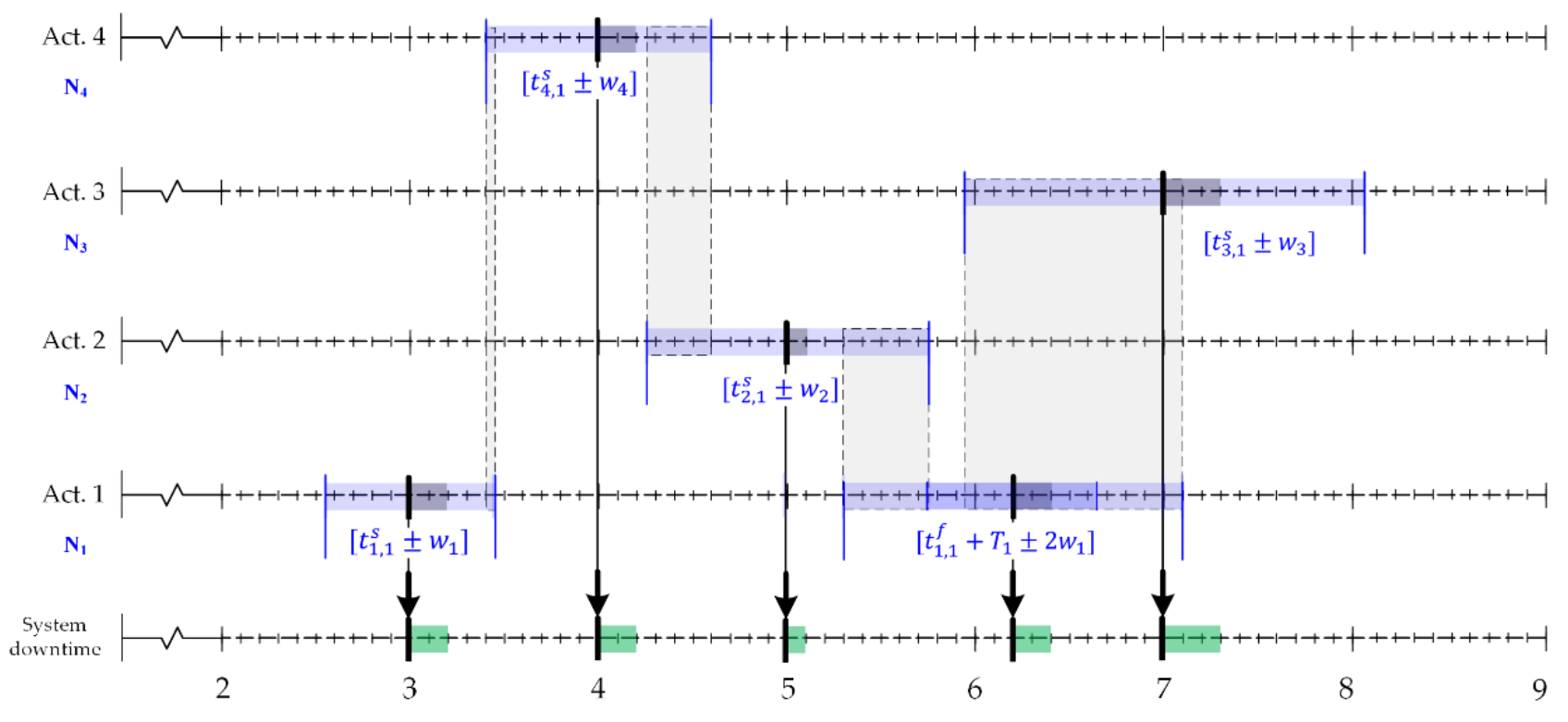
Figure 4 represents a preliminary grouping scheme through the application of Algorithm 1, considering the initial instance where . The intervals colored in blue represent the time-window tolerances, while the grey intervals represent the proposed intersections for each activity. In this scenario, the number of preliminary grouping pairs established and stored in the set corresponds to . As observed in Figure 4, the time window for execution (1,2) depends directly on the execution time of the previous execution . For example, if is assigned, then its feasibility will depend exclusively on the use of the tolerance time windows (i.e., an execution delaying) of the previous execution . Implementing Algorithm 1 for all the generated instances, the set of total grouping pairs delivers , maintaining the preliminary results from the initial instance.
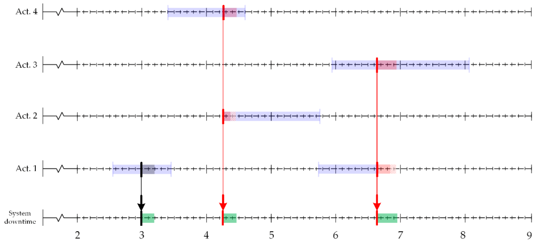
The grouping scheme of the previous initial solution delivers five maintenance interventions with a system availability equivalent to 1.0 (t.u.). The feasible solution associated with the tentative maintenance plan is given by ; . The feasible grouping scheme presented in Figure 5 is depicted by the set . This feasible solution is traduced into system unavailability of 0.7 (t.u.), thus generating three interventions in total. Considering that the initial execution for execution corresponds to , the time-window tolerance considered for is reduced, discarding the feasibility of grouping the pair , thus forcing .
The proposed grouping schemes still allow a further reduction in system unavailability. Figure 6 establishes the optimal solution for the illustrative example, considering the solution , generating three system interventions with total unavailability of 0.6 (t.u.). The new optimized scenario establishes a 40% reduction in the downtime associated with the base scenario derived from Figure 4, allowing substantial savings in fixed maintenance costs and considerably improving the availability of the production system.
2.2.3. An Optimization Model for the Maintenance Grouping Framework
Based on the proposed framework, the optimization model considers the following decision variables and parameters (See Table 3).
The following optimization model is formulated under the mixed-integer linear programming (MILP) paradigm. The model considers the following set of constraints for the use of time-window tolerances for the opportunistic grouping scheme:
s.t.
Under the utilization of constraints (9) and (10), it is possible to limit the execution time according to the width of the specified time window for each execution . The set of constraints (11)–(16) establishes the adaptation of the base formulation for the application of the grouping strategy with time windows of tolerances, according to Mena et al. [46].
To correctly quantify the downtimes associated with each execution pair in the event of grouping schemes, it is necessary to incorporate the following sets of additional constraints to the base formulation. The set of constraints (17)–(19) establishes in a first instance suitable lower bounds for the measurement of . In this way, if a certain execution belongs to a work package, then the constraints (17) and (18) state that
Otherwise, the expression satisfies that , through constraint (19). Constraints (20)–(22) establish several upper bounds to control the growth of the variable , through the incorporation of the auxiliary binary variables and , avoiding an overestimation of the unavailability associated with each execution. In this sense, constraint set (23) ensures that for the set of variables , only one of them is activated for each pair , establishing precisely the best adjusted upper bound, so that the expression (27) is translated into:
In this way, the set of constraints (17)–(23) allows a correct assignment of the downtime values through variable . Constraints (24) and (25) limit the growth of these variables in the absence of grouping schemes, so that , if . Therefore, constraints (16)–(25) generate the following behavior: if the tuple is grouped, then its associated downtime corresponds to the expression (28); otherwise, this time corresponds to . Additionally, constraint (26) is proposed to correctly count the unavailability associated with each work package only once. Finally, the objective function corresponds to the minimization of expression (8). In this way, the counting of corresponds exactly to the unavailability of the system, so that expression (8) corresponds to the minimization of the system’s downtime. In summary, the model conformed by the objective function (8) and constraints (9)–(26) corresponds to the optimization model for the opportunistic grouping framework proposed in Section 2.2.1.
2.2.4. Computational Implementation and Optimization Settings
The framework presented in Section 2.2.3 responds to the MILP mathematical programming paradigm, whose computational implementation has been widely extended in optimization problems, especially on operations and maintenance management, including the planning and scheduling phases, logistics, distribution, and multi-product optimization [50]. In decision-based optimization problems, it is common to incorporate not only quantities attributable to continuous variables but also discrete variables and non-linearities that can be replaced by piecewise linearizations [50]. In these cases, the MILP paradigm is adjusted responding to the requirements through Linear Programming-base Branch and Bound solvers, which allow, in addition to the generation of strict upper and lower bounds, to obtain performance metrics regarding the optimization of the solutions obtained, improving computing times, and decreasing computational costs through the decision tree pruning of integrality constraints [51]. In this way, these algorithms are characterized by the obtention of deterministic optimal solutions, considering only exact parametrizations.
Despite the approach of these algorithms, a variety of highly complex problems, including maintenance activity grouping problems [52], can offer a large number of ramifications of the decision tree, reducing the quality of upper and lower bounds, and therefore generating a suboptimal solution [50]. However, new commercial alternatives combine sophisticated techniques that combine the use of Branch and Bound algorithms with Branch and Cut, e.g., engines such as CPLEX or Gurobi. Using commercial optimization engines to solve the MILP model, the programming stages are described in detail below:
- Definition of instance sets and parameters: In the first stage, the script defines the parametric set that characterizes the instance presented through the PM plan in Section 2.1. This implies incorporating information such as the number and frequency of activities, the execution tolerance factors, and repair times per activity.
- Embedding MILP solver: The Gurobi solver is implemented using Python programming language for its optimization and obtaining results. To do this, a general optimization instance is defined over which the sets of constraints that make up the formulated framework are loaded. The optimization engine is executed under standard searching settings, aiming at an intensification strategy to improve the optimality of the solution found, at the expense of higher computing times.
- Determination of performance indicators and rendering process: Once the best solution found by the Gurobi solver has been obtained, the results are compiled and stored in sorted list-type data, on which the information of each of the performance indicators is obtained according to the definition specified in Section 3. To calculate these indicators, the use of specialized programming packages is considered to manipulate the data using real intervals, allowing the operations of union and intersection of sets in the system unavailability estimation. The graphic material is then rendered under the Python programming language, using the information stored from the compilation.
3. Results
The computational results were measured through a 2.6 GHz processor and 8 GB of built-in RAM, considering a 64-bit architecture. The implementation was carried out using the Gurobi optimization solver, embedded with Pyomo programming language. Different performance indicators were considered to measure and quantify the results of each maintenance plan, under several tolerance factors. In addition to the system availability indicators and related indicators, it is also relevant to measure the effective use of the tolerance time windows, with respect to the estimated optimal grouping scheme. In this sense, the following percentage indicators of average advancement and average delay of the activities are presented in (29)–(30), where the sets and exclusively consider the number of early or late execution pairs , respectively:
Additionally, the percentage frequencies of advanced, delayed, and conservative executions of PM activities will be reported as auxiliary indicators for each instance. These performance indicators are defined through the expressions (31)–(33) as follows:
Considering the complexity in the representation of the instances, as well as the difficulty of presenting them explicitly, the results of the computational implementation under several tolerance factors are summarized in Table 4. For the implementation of the grouping strategy, it was considered an annual planning horizon (52 weeks), and a maximum tolerance factor of 5%, according to the standard percentages proposed in [46]. According to the reported optimality gap, results reveal that the optimization model has reached optimal solutions for each one of the instances. Simultaneously, a consistent increase in the tolerance factor offers, in turn, a progressive decrease in the system unavailability. The results show the capacity of the formulated framework to generate new grouping schemes as the tolerance factor increases. This observation is corroborated by the progressive decrease in the number of activities carried out on their tentative date. Alternatively, the performance indicators and do not show a systematic behavior related to the tolerance factor, as well as and .
Additionally, the results show an increase in the computing times related to each optimal solution as the tolerance factor increases. This is directly related to the increase in the number of feasible grouping schemes as the time-window tolerances increase their width for each execution pair. Therefore, an increase in the number of grouping schemes implies a greater number of decision variables. However, the computing processing times do not exceed more than 1(s) to solve the optimality problem, which is not a limitation for solving grouping schemes to optimality in reasonable computational times.
Table 5 presents the results of unavailability by scenario, and the reduction of inefficiency, measured as the percentual difference between the system unavailability reported from the initial solution with null tolerance factor (i.e., tentative execution plan), and the unavailability reported by the optimal solution. As observed in the previous results, the reduction of inefficiency through the application of the framework increases progressively as the tolerance factor increases, achieving a reduction of 26% in the downtime of the system under a 5% tolerance factor, reducing unavailability from eight weeks to six weeks. Additionally, what is observed is a decrease in the progressive reduction of inefficiency by consecutively reaching a higher tolerance factor. For example, going from 2% to 3% in the increase of the allowable tolerance causes an increase of almost 6% in the reduction of inefficiency, while going from 4% to 5% only reports a 0.2% in the reduction of unavailability.
The use of the tolerance time windows, as well as the assignment of the execution times and conformed grouping schemes, can be presented employing a Gantt chart-based representation, according to the nomenclature presented in Figure 3. Figure 7 represents the base PM plan of the critical activities analyzed for a planning horizon of 52 weeks. As observed, system stoppages are represented by grey vertical lines, while system unavailability is represented by green bars. The initial tentative maintenance plan includes a total of 35 stoppages, generating system unavailability of approximately 8 weeks per year.
If the application of a tolerance factor of 5% is now considered, then the number of stoppages is reduced to 19, which implies an inefficiency reduction of almost 30%, compared to the base case, which offers a gain equivalent of two-week system availability per year. What is observed in this scenario (See Figure 8) is the use of the time-window tolerances for the generation of grouping schemes, thus allowing to considerably reduce the number of interruptions while increasing the availability of the system.
4. Discussion
Although the results obtained from the computational implementation are consistent, it is necessary to discuss the limitations and computational complexity issues that the framework includes. In the first term, the values associated with the deviation indicators from the tentative maintenance plan cannot be underestimated. Although the optimal maintenance plan establishes a considerable reduction in the unavailability of the system as the tolerance factor increases, the number of activities maintaining their tentative execution date does not exceed 20% of the total executions.
In this sense, it is necessary to consider that the deviation from the tentative execution date of the PM activities implies a risk: the advance of activities on its part implies a poor economic performance, while its delay may increase the probability of failure occurrence in certain assets [52]. This may bring a considerable impact on the degradation of the assets, and therefore, on the probability of critical failures of the components if a previous estimation of the tolerance factor is undertaken. Hence the need to estimate, based on advanced optimization techniques and expert recommendations, the use of tolerance based on a controlled risk zone, which does not involve malfunctions that affect the economic performance of the plant, as well as the potential failures that may put the health of the personnel and the environment at risk.
On the other hand, it is necessary to discuss the resolution times reported in the computational implementation. Although the different instances have reported a reasonable computing time, what is observed is a consistent increase in the number of decision variables, as well as in the number of constraints and the computing times reported (See Figure 9). This must be taken into account when considering an increase in the number of PM activities to plan and schedule, which may eventually cause an increase in computing times or a suboptimal grouping scheme. In this sense, it is necessary to establish that the size of the MILP model previously presented, and therefore its complexity does not depend exclusively on the tolerance factor.
Considering that the proposed MILP model is implemented through the use of a commercial solver, what is proposed as a measure of complexity is a theoretical expression for calculating the maximum number of variables and constraints, which directly depend on the number of executions, and indirectly, on the number and periodicity of activities, as well as the tolerance of execution of each one of them. In order to quantify the problem complexity, consider the following expression for the determination of the number of variables and constraints involved in the framework. Let the quantities , , , and be defined as:
Then it is possible to calculate, considering the set of values , the maximum theoretical number of variables and constraints, considering the limit case when (i.e., there are no grouping feasibility constraints by the use of tolerance time windows). Table 6 shows the experimental values and the maximum theoretical value for the evaluated instance, considering that . As can be seen, the number of variables and constraints increases progressively and approaches to maximum theoretical values when the tolerance factor increases. This makes it possible to quantify the level of complexity of the formulated framework, and also evidence the combinatorial explosion phenomenon detected in [46].
The size and complexity of the model depend directly on the total number of executions to be planned, and the latter depends in turn on a variety of parameters, including the execution periodicity, the number of activities to be planned, as well as the length of the planning horizon. In this sense, it is important to observe that the grouping problem presented here can be conceived as a variant of the Set Covering Problem, a problem widely documented as an NP-Hard class problem [53,54]. In this sense, it is necessary to take into account the occurrence of the combinatorial explosion phenomenon for larger instances [46,52].
Additionally, the above-analyzed framework considers an unlimited availability of resources for its execution. In a scenario of scarce availability of resources, the optimal maintenance plan presented here may have to undergo considerable modifications. In this case, it will be necessary to include new decision variables that address the problem of resource allocation, thus considerably increasing the complexity levels and computational tractability of the optimization model previously presented.
5. Conclusions and Managerial Recommendations
The research proposes the framework formulation and optimization model for the opportunistic grouping strategy in the planning of preventive maintenance activities for a wastewater treatment plant. A review of the operating context, as well as the formulation of the framework and the respective optimization model, is addressed in detail through this research. The computational results from the implementation of the model reveal in turn a considerable decrease in the level of unavailability associated with the primary treatment line and sludge treatment, which implies the potential to greater cost-efficiency and an increase in productivity and performance levels through optimized strategies for maintenance management in the WWTP under analysis.
However, it is necessary to consider the limitations and the challenges that the framework formulation pose, among which are the consideration of a fixed periodicity under perfect maintenance assumption, and the incapability to stochastically include the failure phenomenon and its impact on maintenance plans. Other challenges posed through this research include: the impact of the maintenance execution and opportunistic groups modeling with multiple failure modes per equipment; the incorporation of different maintenance policies and grouping strategies with a focus on repairable systems; and alternatively, the possibility of modeling degradation, along with stochastic and structural interaction of the components involved in the complex production systems. These limitations in turn represent research lines and suggestive challenges that will be addressed in future research, which are directly related to the capacity of the framework to improve its flexibility, adherence, and applicability of the grouping strategy in several industrial settings.
Based on the computational implementation and the obtained results, several recommendations and insights focused on the maintenance management decision-making are presented below:
- The maintenance grouping framework must be applied, restructured, and updated periodically to ensure effectiveness as an operational support tool. Said update process must be managed both at an operational level, (through the requirements of parts and pieces, personnel qualification, and repair and logistic-delay times) as well as at a tactical level, (e.g., faced with the incorporation or redesign of tasks through maintenance plan design tools such as Reliability Centered Maintenance).
- The framework assumes that components can necessarily share fixed setup costs through the clustering process. This information must be corroborated at a tactical level, by reviewing the procedures for the execution of PM activities, as well as the effect of said activities on the productivity level or on the treatment plant cost function. Otherwise, the framework formulated will not allow to optimally improve the cost-efficiency of the current maintenance plan.
- It is also assumed that a certain work package can share a setup cost, regardless of the number of grouped components. This necessarily implies that the more components are added to a group, the greater the fixed maintenance cost savings. However, the structure of fixed maintenance costs is generally complex, and besides, the availability of resources is generally scarce and limited. Additionally, there may be activities that may not eventually be grouped due to the existence of technical constraints (assembly/disassembly procedures, technical infeasibility due to physical/layout limitations). In this case, it is necessary to review the implementation of new constraints to ensure the grouping feasibility and the application of resource and budgetary restrictions. Future research works aim to address the aspects mentioned above to consistently improve the applicability of the framework in different industrial settings.
- Regarding the relationship between the framework and risk management, the evidence shows the exclusion of uncertainty metrics when defining risk, and the lack of a clear definition of probability obtained in the risk assessment standards for sewage treatment systems. Considering that the tolerance level implicitly establishes a certain risk-acceptance level, it is important to establish the risk tolerance that the system can allow without affecting the performance of the treatment plant. In this regard, it is relevant to set the execution tolerance level based on the expertise, using tools such as single-component multi-attribute optimization with a focus on risk management. In this regard, it is important to consider the dependencies or critical interactions between the components of the system, considering at least three main consequence types: fatalities, injuries, and economic losses, which must be estimated on organizations, environment, and stakeholders.
Author Contributions
Conceptualization, P.V., L.M. and R.M.; methodology, P.V. and R.M.; software, L.M.; validation, P.V. and L.M.; formal analysis, P.V. and R.M.; investigation, P.V. and R.M.; resources, F.K.; data curation, L.M.; writing—original draft preparation, L.M. and P.V.; writing—review and editing, P.V.; visualization, L.M.; supervision, F.K. and P.V.; project administration, P.V.; funding acquisition, F.K. All authors have read and agreed to the published version of the manuscript.
Funding
This research received no external funding.
Institutional Review Board Statement
Not applicable.
Informed Consent Statement
Not applicable.
Conflicts of Interest
The authors declare no conflict of interest.
References
- Coit, D.W.; Zio, E. The evolution of system reliability optimization. Reliab. Eng. Syst. Saf. 2019, 192, 106259. [Google Scholar] [CrossRef]
- Garetti, M.; Taisch, M. Sustainable manufacturing: Trends and research challenges. Prod. Plan. Control 2012, 23, 83–104. [Google Scholar] [CrossRef]
- Sharma, A.; Yadava, G.; Deshmukh, S.G. A literature review and future perspectives on maintenance optimization. J. Qual. Maint. Eng. 2011, 17, 5–25. [Google Scholar] [CrossRef]
- Ansari, F.; Fathi, M.; Seidenberg, U. Problem-solving approaches in maintenance cost management: A literature review. J. Qual. Maint. Eng. 2016, 22, 334–352. [Google Scholar] [CrossRef]
- de Jonge, B.; Scarf, P.A. A review on maintenance optimization. Eur. J. Oper. Res. 2020, 285, 805–824. [Google Scholar] [CrossRef]
- Alrabghi, A.; Tiwari, A. State of the art in simulation-based optimisation for maintenance systems. Comput. Ind. Eng. 2015, 82, 167–182. [Google Scholar] [CrossRef] [Green Version]
- Ding, S.-H.; Kamaruddin, S. Maintenance policy optimization—literature review and directions. Int. J. Adv. Manuf. Technol. 2015, 76, 1263–1283. [Google Scholar] [CrossRef]
- Hernández-Chover, V.; Castellet-Viciano, L.; Hernández-Sancho, F. Preventive maintenance versus cost of repairs in asset management: An efficiency analysis in wastewater treatment plants. Process. Saf. Environ. Prot. 2020, 141, 215–221. [Google Scholar] [CrossRef]
- Ozgun, H.; Cicekalan, B.; Akdag, Y.; Koyuncu, I.; Ozturk, I. Comparative evaluation of cost for preliminary and tertiary municipal wastewater treatment plants in Istanbul. Sci. Total Environ. 2021, 778, 146258. [Google Scholar] [CrossRef]
- Henderson, B.; Bui, E. Ecological Risk Assessment. In Risk Assessment; John Wiley & Sons: Hoboken, NJ, USA, 2012; pp. 26–55. ISBN 978-1-118-30962-9. [Google Scholar]
- Hernández-Chover, V.; Bellver-Domingo, Á.; Hernández-Sancho, F. Efficiency of wastewater treatment facilities: The influence of scale economies. J. Environ. Manag. 2018, 228, 77–84. [Google Scholar] [CrossRef]
- Hamza, R.A.; Iorhemen, O.T.; Tay, J.H. Advances in biological systems for the treatment of high-strength wastewater. J. Water Process. Eng. 2016, 10, 128–142. [Google Scholar] [CrossRef]
- Riffat, R. Fundamentals of Wastewater Treatment and Engineering; CRC Press: Boca Raton, FL, USA, 2012; ISBN 978-0-203-81571-7. [Google Scholar]
- Dauknys, R.; Rimeika, M.; Jankeliūnaitė, E.; Mažeikienė, A. Disintegration impact on sludge digestion process. Environ. Technol. 2016, 37, 2768–2772. [Google Scholar] [CrossRef]
- Hu, Y.; Yang, Y.; Zang, Y.; Zhang, J.; Wang, X. Anaerobic dynamic membrane bioreactors (AnDMBRs) for wastewater treatment. In Current Developments in Biotechnology and Bioengineering; Elsevier: Amsterdam, The Netherlands, 2020; pp. 259–281. ISBN 978-0-12-819852-0. [Google Scholar]
- Lazarus, W.F.; Rudstrom, M. The Economics of Anaerobic Digester Operation on a Minnesota Dairy Farm. Rev. Agric. Econ. 2007, 29, 349–364. [Google Scholar] [CrossRef]
- Rajendran, K.; Lin, R.; Wall, D.M.; Murphy, J.D. Influential Aspects in Waste Management Practices. In Sustainable Resource Recovery and Zero Waste Approaches; Elsevier: Amsterdam, The Netherlands, 2019; pp. 65–78. [Google Scholar]
- Brancoli, P.; Bolton, K. Life Cycle Assessment of Waste Management Systems. In Sustainable Resource Recovery and Zero Waste Approaches; Elsevier: Amsterdam, The Netherlands, 2019; pp. 23–33. ISBN 978-0-444-64200-4. [Google Scholar]
- Liao, X.; Li, H.; Cheng, Y.; Chen, N.; Li, C.; Yang, Y. Process performance of high-solids batch anaerobic digestion of sewage sludge. Environ. Technol. 2014, 35, 2652–2659. [Google Scholar] [CrossRef]
- Griffin, M.E.; McMahon, K.D.; Mackie, R.I.; Raskin, L. Methanogenic Population Dynamics during Start-up of An-aerobic Digesters Treating Municipal Solid Waste and Biosolids. Biotechnol. Bioeng. 1998, 57, 14. [Google Scholar] [CrossRef]
- Foresti, E. Perspectives on anaerobic treatment in developing countries. Water Sci. Technol. 2001, 44, 141–148. [Google Scholar] [CrossRef]
- Brown, R.; Willis, H. The economics of aging infrastructure. IEEE Power Energy Mag. 2006, 4, 36–43. [Google Scholar] [CrossRef]
- Johnson, J.L. Our Infrastructure is Aging and Maintenance Costs are Rising—Extending the Life Expectancy of Transmission Lines Through the Use of Data, Inspection and Planning. In Proceedings of the ESMO 2006—2006 IEEE 11th International Conference on Transmission & Distribution Construction, Operation and Live-Line Maintenance, Albuquerque, NM, USA, 15–20 October 2006; IEEE: Piscataway, NJ, USA, 2006; p. 4144516. [Google Scholar]
- Hukka, J.J.; Katko, T.S. Resilient Asset Management and Governance Fordeteriorating Water Services Infrastructure. Procedia Econ. Financ. 2015, 21, 112–119. [Google Scholar] [CrossRef] [Green Version]
- Gunn, E.; Diallo, C. Optimal Opportunistic Indirect Grouping of Preventive Replacements in Multicomponent Sys-tems. Comput. Ind. Eng. 2015, 90, 281–291. [Google Scholar] [CrossRef]
- Do, P.; Vu, H.C.; Barros, A.; Berenguer, C. Maintenance grouping for multi-component systems with availability constraints and limited maintenance teams. Reliab. Eng. Syst. Saf. 2015, 142, 56–67. [Google Scholar] [CrossRef] [Green Version]
- Nguyen, H.S.H.; Do, P.; Vu, H.-C.; Iung, B. Dynamic maintenance grouping and routing for geographically dispersed production systems. Reliab. Eng. Syst. Saf. 2019, 185, 392–404. [Google Scholar] [CrossRef]
- Thomas, L. A survey of maintenance and replacement models for maintainability and reliability of multi-item systems. Reliab. Eng. 1986, 16, 297–309. [Google Scholar] [CrossRef]
- Hameed, Z.; Vatn, J. Role of grouping in the development of an overall maintenance optimization framework for offshore wind turbines. Proc. Inst. Mech. Eng. Part O J. Risk Reliab. 2012, 226, 584–601. [Google Scholar] [CrossRef]
- Zhou, X.; Lu, Z.; Xi, L. Preventive maintenance optimization for a multi-component system under changing job shop schedule. Reliab. Eng. Syst. Saf. 2012, 101, 14–20. [Google Scholar] [CrossRef]
- Xia, T.; Xi, L.; Zhou, X.; Lee, J. Dynamic maintenance decision-making for series–parallel manufacturing system based on MAM–MTW methodology. Eur. J. Oper. Res. 2012, 221, 231–240. [Google Scholar] [CrossRef]
- Van, P.D.; Barros, A.; Berenguer, C.; Bouvard, K.; Brissaud, F. Dynamic grouping maintenance with time limited opportunities. Reliab. Eng. Syst. Saf. 2013, 120, 51–59. [Google Scholar] [CrossRef]
- Pandey, M.; Zuo, M.J.; Moghaddass, R. Selective maintenance scheduling over a finite planning horizon. Proc. Inst. Mech. Eng. Part O J. Risk Reliab. 2016, 230, 162–177. [Google Scholar] [CrossRef]
- Zhu, W.; Castanier, B.; Bettayeb, B. A dynamic programming-based maintenance model of offshore wind turbine considering logistic delay and weather condition. Reliab. Eng. Syst. Saf. 2019, 190, 106512. [Google Scholar] [CrossRef]
- Wu, T.; Yang, L.; Ma, X.; Zhang, Z.; Zhao, Y. Dynamic maintenance strategy with iteratively updated group information. Reliab. Eng. Syst. Saf. 2020, 197, 106820. [Google Scholar] [CrossRef]
- Zhou, X.; Yu, M. Semi-dynamic maintenance scheduling for multi-station series systems in multi-specification and small-batch production. Reliab. Eng. Syst. Saf. 2020, 195, 106753. [Google Scholar] [CrossRef]
- Nourelfath, M.; Châtelet, E. Integrating production, inventory and maintenance planning for a parallel system with dependent components. Reliab. Eng. Syst. Saf. 2012, 101, 59–66. [Google Scholar] [CrossRef]
- Xiao, L.; Zhang, X.; Tang, J.; Zhou, Y. Joint optimization of opportunistic maintenance and production scheduling considering batch production mode and varying operational conditions. Reliab. Eng. Syst. Saf. 2020, 202, 107047. [Google Scholar] [CrossRef]
- Bertolini, M.; Mezzogori, D.; Zammori, F. Comparison of new metaheuristics, for the solution of an integrated jobs-maintenance scheduling problem. Expert Syst. Appl. 2019, 122, 118–136. [Google Scholar] [CrossRef]
- Zhou, X.; Shi, K. Capacity failure rate based opportunistic maintenance modeling for series-parallel multi-station manufacturing systems. Reliab. Eng. Syst. Saf. 2019, 181, 46–53. [Google Scholar] [CrossRef]
- Chen, X.; Zhang, L.; Zhang, Z. An integrated model for maintenance policies and production scheduling based on immune–culture algorithm. Proc. Inst. Mech. Eng. Part O J. Risk Reliab. 2020, 234, 651–663. [Google Scholar] [CrossRef]
- Dao, C.; Zuo, M.J. Selective maintenance of multi-state systems with structural dependence. Reliab. Eng. Syst. Saf. 2017, 159, 184–195. [Google Scholar] [CrossRef]
- Vijayan, V.; Chaturvedi, S.K. Multi-component maintenance grouping optimization based on stochastic dependency. Proc. Inst. Mech. Eng. Part O J. Risk Reliab. 2021, 235, 293–305. [Google Scholar] [CrossRef]
- Lu, B.; Zhou, X. Opportunistic preventive maintenance scheduling for serial-parallel multistage manufacturing systems with multiple streams of deterioration. Reliab. Eng. Syst. Saf. 2017, 168, 116–127. [Google Scholar] [CrossRef]
- Fan, D.; Zhang, A.; Feng, Q.; Cai, B.; Liu, Y.; Ren, Y. Group maintenance optimization of subsea Xmas trees with stochastic dependency. Reliab. Eng. Syst. Saf. 2021, 209, 107450. [Google Scholar] [CrossRef]
- Mena, R.; Viveros, P.; Zio, E.; Campos, S. An optimization framework for opportunistic planning of preventive maintenance activities. Reliab. Eng. Syst. Saf. 2021, 215, 107801. [Google Scholar] [CrossRef]
- Bodik, I.; Kubaská, M. Energy and sustainability of operation of a wastewater treatment plant. Environ. Prot. Eng. 2013, 39. [Google Scholar] [CrossRef]
- Di Fraia, S.; Massarotti, N.; Vanoli, L.; Costa, M. Thermo-economic analysis of a novel cogeneration system for sewage sludge treatment. Energy 2016, 115, 1560–1571. [Google Scholar] [CrossRef]
- Sadhukhan, J. Distributed and micro-generation from biogas and agricultural application of sewage sludge: Comparative environmental performance analysis using life cycle approaches. Appl. Energy 2014, 122, 196–206. [Google Scholar] [CrossRef] [Green Version]
- Grossmann, I.E. Challenges in the application of mathematical programming in the enterprise-wide optimization of process industries. Theor. Found. Chem. Eng. 2014, 48, 555–573. [Google Scholar] [CrossRef]
- Wolsey, L. Integer Programming, 1st ed.; Wiley: Hoboken, NJ, USA, 2020; ISBN 978-1-119-60647-5. [Google Scholar]
- Do, P.; Barros, A. Maintenance grouping models for multicomponent systems. In Mathematics Applied to Engineering; Elsevier: Amsterdam, The Netherlands, 2017; pp. 147–170. ISBN 978-0-12-810998-4. [Google Scholar]
- Korte, B.; Vygen, J. Chapter 16: Approximation Algorithms. In Combinatorial Optimization; Algorithms and Combinatorics; Springer: Berlin/Heidelberg, Germany, 2012; Volume 21, p. 414. ISBN 978-3-642-24487-2. [Google Scholar]
- Vu, H.C.; Do, P.; Barros, A.; Berenguer, C. Maintenance grouping strategy for multi-component systems with dynamic contexts. Reliab. Eng. Syst. Saf. 2014, 132, 233–249. [Google Scholar] [CrossRef]
Figure 1.
Wastewater treatment process diagram for the case study. Source: Own elaboration.

Figure 2.
Anaerobic digestion process for the case study.

Figure 3.
(a) Impact of the grouping strategy on the periodicity and tentative executions; (b) impact of grouping schemes over the system unavailability.
Figure 3.
(a) Impact of the grouping strategy on the periodicity and tentative executions; (b) impact of grouping schemes over the system unavailability.

Figure 4.
Representation of the use of tolerances for the generation of feasible grouping schemes.

Figure 5.
Illustrative example. Grouping scheme for a feasible solution.

Figure 6.
Application example. Schematic representation of the optimal solution for the instance.

Figure 7.
Optimal grouping schemes for the case study under tolerance factor , considering a 52-week planning horizon. (a) First semester (weeks 1–26); (b) Second semester (weeks 27–52).
Figure 7.
Optimal grouping schemes for the case study under tolerance factor , considering a 52-week planning horizon. (a) First semester (weeks 1–26); (b) Second semester (weeks 27–52).

Figure 8.
Optimal grouping schemes for the case study under a tolerance factor , considering a 52-week planning horizon. (a) First semester (weeks 1–26); (b) Second semester (weeks 27–52).
Figure 8.
Optimal grouping schemes for the case study under a tolerance factor , considering a 52-week planning horizon. (a) First semester (weeks 1–26); (b) Second semester (weeks 27–52).

Figure 9.
Computing times under several tolerance factor values. WWTP case study.


Table 1.
Preventive maintenance plan for highly critical and hazardous activities. Case study.
| ID | Area/Process | Activity Description | Execution Periodicity (w) | Execution Time (h) |
|---|---|---|---|---|
| 1 | Roughing | Inspection of sensor chains and electrical connections | 20 | 8 |
| 2 | Grit removal | Inspection of aerators for desanding process | 48 | 8 |
| 3 | Roughing Grit Removal | Change of luminaires | 36 | 5 |
| 4 | Grit removal | Bridge repair | 18 | 96 |
| 5 | Mixing | Inspections and unclogging of submersible pumps | 15 | 24 |
| 6 | Homogeneization | Agitator check | 10 | 24 |
| 7 | Deodorization | Tower cleaning | 50 | 72 |
| 8 | Gas flow line | Equipment maintenance | 4 | 72 |
| 9 | Electrical distribution | Scheduled inspection of medium voltage equipment | 1 | 1 |
| 10 | Dehydration | Inspection of agitator and electrical cables | 12 | 24 |
| 11 | Electrical distribution | MT switchgear | 30 | 1 |
| 12 | Sludge digestion | Check flow meters and gas flow leaks in purge chambers | 24 | 4 |
| 13 | Sludge digestion—Digester room | Checking and cleaning the heat exchanger and controller | 20 | 6 |
| 14 | Sludge digestion | Temperature probe and thermostat inspection | 28 | 2 |
| 15 | Sludge digestion—Digester room | Three-way valve and actuator inspection | 35 | 5 |
Table 2.
Application example. Instance specifications.
| Sets and Parameters | Notation | Value |
| Planning horizon | 8 | |
| Execution tolerance | ||
| Scheduled activities | 4 | |
| Activity | Periodicity (t.u.) | Execution time (t.u.) |
| 1 | 3 | 0.2 |
| 2 | 5 | 0.1 |
| 3 | 7 | 0.3 |
| 4 | 4 | 0.2 |
Table 3.
Summary and description of decision variables.
| Decision Variable | Description | Nature |
|---|---|---|
| Start time for the -th execution of activity | ||
| Resumption time for the -th execution of activity | ||
| Detention time assigned to the -th execution of activity | ||
| Auxiliary variable for downtime accountability related with the -th execution of activity | ||
| Binary grouping variable, where if the -th execution for activity is part of the group linked to the -th execution of activity | ||
| Auxiliary variable | ||
| Auxiliary variable |
Table 4.
Performance indicators for instances under several tolerance factors.
| (%) | Best Value (Weeks) | Optimality GAP (%) | Resolution Time (s) | |||||
|---|---|---|---|---|---|---|---|---|
| 0.00 | 7.98 | 0 | 0 | 0 | 0 | 0 | 0 | 100 |
| 1.00 | 7.59 | 0 | 0.1327 | 11.20 | 27.79 | 39.53 | 37.91 | 32.56 |
| 2.00 | 7.45 | 0 | 0.3022 | 10.57 | 32.15 | 44.18 | 30.23 | 25.58 |
| 3.00 | 6.87 | 0 | 0.3352 | 21.58 | 18.74 | 32.56 | 46.51 | 20.93 |
| 4.00 | 5.89 | 0 | 0.6390 | 35.87 | 12.04 | 23.25 | 55.81 | 20.93 |
| 5.00 | 5.87 | 0 | 0.9753 | 20.78 | 26.92 | 37.21 | 46.51 | 16.28 |
Table 5.
Results of unavailability of the system and reduction of inefficiency, for different tolerance factors.
Table 5.
Results of unavailability of the system and reduction of inefficiency, for different tolerance factors.
| (%) | System Unavailability (Weeks) | Inefficiency Reduction (%) |
|---|---|---|
| 0.00 | 7.98 | - |
| 1.00 | 7.59 | 4.6 |
| 2.00 | 7.45 | 6.6 |
| 3.00 | 6.87 | 13.9 |
| 4.00 | 5.89 | 26.2 |
| 5.00 | 5.87 | 26.4 |
Table 6.
Number of variables and constraints under several tolerance factor values ().
| Case | Number of Total Variables | Number of Binary Variables | Number of Continuous Variables | Number of Constraints |
|---|---|---|---|---|
| Theoretical | ||||
| 351 | 179 | 172 | 679 | |
| 441 | 269 | 172 | 978 | |
| 501 | 329 | 172 | 1196 | |
| 531 | 359 | 172 | 1305 | |
| 579 | 407 | 172 | 1487 | |
| 624 | 452 | 172 | 1663 | |
| Max. Theoretical | 2924 | 2752 | 172 | 13,287 |
Publisher’s Note: MDPI stays neutral with regard to jurisdictional claims in published maps and institutional affiliations. |
© 2021 by the authors. Licensee MDPI, Basel, Switzerland. This article is an open access article distributed under the terms and conditions of the Creative Commons Attribution (CC BY) license (https://creativecommons.org/licenses/by/4.0/).
Share and Cite
MDPI and ACS Style
Viveros, P.; Miqueles, L.; Mena, R.; Kristjanpoller, F. Opportunistic Strategy for Maintenance Interventions Planning: A Case Study in a Wastewater Treatment Plant. Appl. Sci. 2021, 11, 10853. https://doi.org/10.3390/app112210853
AMA Style
Viveros P, Miqueles L, Mena R, Kristjanpoller F. Opportunistic Strategy for Maintenance Interventions Planning: A Case Study in a Wastewater Treatment Plant. Applied Sciences. 2021; 11(22):10853. https://doi.org/10.3390/app112210853
Chicago/Turabian StyleViveros, Pablo, Leonardo Miqueles, Rodrigo Mena, and Fredy Kristjanpoller. 2021. "Opportunistic Strategy for Maintenance Interventions Planning: A Case Study in a Wastewater Treatment Plant" Applied Sciences 11, no. 22: 10853. https://doi.org/10.3390/app112210853
Note that from the first issue of 2016, this journal uses article numbers instead of page numbers. See further details here.