
Influence of Posture Change on Train Running Safety under Crosswind
by
 ,
,
Jian Yan
1,*, 
Tefang Chen
1,
Shu Cheng
1,
E Deng
2,*,
Weichao Yang
2,
Shuaihan Guo
1 and
Zijian Guo
1 1
School of Traffic & Transportation Engineering, Central South University, Changsha 410075, China
2
School of Civil Engineering, Central South University, Changsha 410075, China
*
Authors to whom correspondence should be addressed.
Appl. Sci. 2021, 11(13), 6067; https://doi.org/10.3390/app11136067
Submission received: 3 June 2021
/
Revised: 14 June 2021
/
Accepted: 24 June 2021
/
Published: 30 June 2021
Abstract
:High-speed trains serving in a crosswind region are bearing more significant safety risks. Based on the three-dimensional (3D) Unsteady Reynolds-Averaged Navier–Stokes (URANS) turbulence model, a Computational Fluid Dynamics (CFD) computational work was conducted in the present study to predict the transient aerodynamic load of the train. The transient aerodynamic load was then employed as the input of the dynamic system to perform a dynamic analysis of running safety. Noticeable changes in the aerodynamic coefficients were found when the train entered and left the crosswind region due to the dramatic change in flow patterns. The original posture also provided significant changes to the train’s aerodynamic responses. A slightly larger maximum derailment coefficient was found on the first bogie of the leading car with a preset posture. There were obvious differences in the displacement characteristics of the three cars in the lateral direction and the rolling rotation, and the magnitude of the posture changes decreased from the leading car to the trailing car. The train with the consideration of posture was proven to withstand weaker crosswinds.
1. Introduction
Trains are becoming a more significant mode of high-speed and cost-effective public transportation for passengers and freight. When a crosswind exists, the running train is subjected to a speed limit [1], which has a significant effect on carrying efficiency. Operational protection is also threatened by the crosswind [2]. In fact, many derailment accidents due to crosswinds have been reported around the world, such as in China [3,4], Japan [5,6], and the UK [7,8]. Furthermore, the vehicle’s violent vibration do not only affect safety but also passenger comfort [9], and can deteriorate vehicle–infrastructure interaction performance [10].
As a result, research into train aerodynamic performance and running safety in crosswinds has become popular [11,12,13]. In response to the train overturning accidents mentioned above, a large number of studies have been carried out through full-scale tests [14], scaled model tests [15,16,17], and numerical simulations [18,19] to study aerodynamic performance, the surrounding flow field distribution, the operational safety of static or dynamic trains, and the effect of wind protection facilities in crosswind regions. Among these, numerical simulation methods have received more attention in recent years [20,21] due to their reliable results, low cost, and easy control of test variables. Static trains are used in the majority of numerical investigations. Although such research approaches have a cheap computational cost and are versatile in terms of computing the flow field around the train, they are unable to replicate the train’s movement when the transient flow field and the crosswind are coupled. As a result, several investigations on trains in crosswinds have been conducted with a dynamic method. The wind–train–bridge coupling is studied using a dynamic analysis model. In the research conducted by Deng et. al. [11], the effects of a wind barrier with a height of 3 m and a porosity of 30% on the aerodynamic coefficient, flow field structure, and running protection of high-speed trains under crosswind are explored in the bridge–tunnel section; results showed that the wind barrier reduced the sharp change effect of the aerodynamic coefficient by more than 50%. Yang et. al. [22] conducted an analysis of the wind–train–bridge dynamic coupled system and the dynamic responses of the train in the tunnel–bridge–tunnel infrastructure in the canyon wind environment were explored. Deng et al. [23] discovered that trains passing through a tunnel in a crosswind experienced transient changes in the flow field structure and aerodynamic characteristics, which reduced the running safety of the train.
It has been proven that the yaw angle has a significant effect on the aerodynamic forces and moments of the train. However, the train is subjected to unbalanced and unstable forces during operation, and its posture is bound to change during the entire operation. Changes in some degrees of freedom, including the yaw attitude that can directly determine the yaw angle, will change the flow field around the train and its aerodynamic performance, thereby affecting the safety of the train’s operation [24]. According to a previous study [25], in terms of vehicle dynamics and as a result of relative lateral displacements in the wheel–rail contact site, primary and secondary suspension between tracks, wheelsets, bogie frames, and car bodies, the gravitational center of bodies will deviate from the central line of track. It was also proven that when a train runs on a bridge suffering a crosswind, its attitude varied, as did the flow field, aerodynamic loads, and running safety indices. However, in the studies of different train postures, only the running on a bridge is considered, which is a relatively specific operating environment. However, a train tends to run more on flat ground, and its aerodynamic response performance and running safety will be different form that on the bridge. Although there are many studies on train dynamics, it is still unknown whether its attitude changes will have a worse impact on safety threats in the common running on flat ground.
Therefore, a three-dimensional (3D) Computational Fluid Dynamics (CFD) model of the train–wind is proposed in the present investigation to study the transient aerodynamic load of each car of the train based on the Unsteady Reynolds-Averaged Navier–Stokes (URANS) turbulence model. A validated dynamic system was used to predict the running safety of the train with and without the given specific posture. The aerodynamic responses of each car of the train passing through the crosswind region with and without the given specific posture were compared and analyzed in terms of the aerodynamic coefficient and flow patterns. The effect of the given posture on train running safety was also considered based on the train derailment coefficient (DC), wheel load reduction rate (WLRR), the time-varying running posture, and their accelerations in five degrees of freedom. The physical model, method, computational domain, boundary conditions, and computational meshes are described in Section 2; the validation is given in Section 3; Section 4 discusses the results; and finally, the conclusion is drawn in Section 5.
2. Numerical Methodology
2.1. Model
Figure 1 shows the train employed in the present study, which is the 1:1 scale Chinese CRH3 high-speed train. To display the difference in the aerodynamic performance of different cars, a leading car, a middle car, and a trailing car were included in the 3-car train; their lengths are 25.78 m, 25.33 m, and 25.78 m, respectively, which makes the entire train 76.9 m long. The height (H) and width of the train are 3.89 m (H) and 3.26 m, respectively. Some geometric details on the train, such as doors, windows, handles, and so on, were ignored to increase the efficiency of grid generation and numerical simulation, while those geometric features that could theoretically affect the train’s dynamic response, such as bogies and inter-carriage gaps, were retained. To replicate the ground clearance provided by the railway track, the train’s lowest end (the lower vertex of the bogie wheelset) was given a 0.2 m distance from the ground.
Based on previous research, different running posture changes were found when the leading car, the middle car, and the trailing car passed through the crosswind area [26]. According to their actual change trends through the wind zone, the posture changes in different degrees of freedom, as in Table 1, are applied to different cars. Note that these attitude changes cannot be accurately assigned due to differences in train geometry, dynamic models, and yaw angles. However, for a more convenient comparison, the rotation angle of each vehicle is increased as a fixed attitude, which is in contrast to the working condition that does not consider the posture change.
2.2. Numerical Method
When simulating flow fields with large Reynolds numbers, various methods such as Large Eddy Simulation (LES) and Detached Eddy Simulation (DES) demonstrate a significant advantage in accurately describing the exact change in flow structures. However, as the mesh resolution and time-step become more rigorous, numerical performance suffers, making it challenging to complete the work in this analysis using these techniques. Additionally, in simulating flow systems analogous to those in this study, the Unsteady Reynolds-Averaged Navier–Stokes (URANS) equations turbulence model is widely used. In the current study, the 3D unsteady RNG k–ε turbulence model was used to simulate the flow field as the train passes through a crosswind region.
The calculations were carried out using the commercial code STAR CCM + 13.06. The pressure data was obtained with the use of a pressure-based solver based on the finite volume method (FVM). A second-order upwind scheme was used to discretize the convection and diffusion concepts. An implied scheme with second-order accuracy was applied to solve the time term, and the time-step was set as 5 × 10⁻⁴ s, giving a courant number less than 1. A total of 20 iterations were implemented in each time-step, and the residual of each turbulent equation was at least 10 × 10−5 at each step.
2.3. Computational Domain and Boundary Conditions
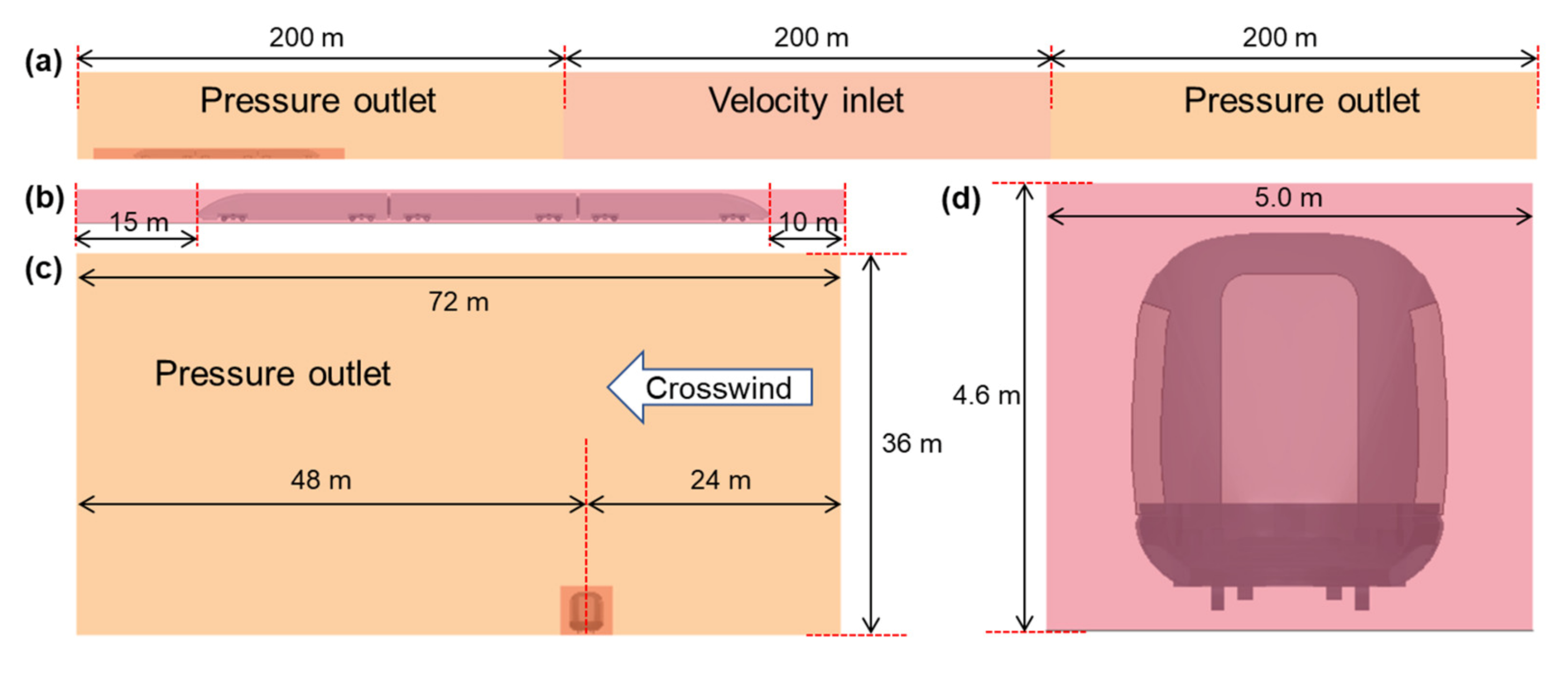
Figure 2 presents the main size and the boundary conditions of the computational domain. The length, width, and height of the calculation domain were 600 m, 72 m, and 36 m, respectively. The train was located 24 m downstream of the inlet, at the width direction of the computational domain, and 0.2 m from the bottom in the height direction. According to the ambient wind situation, the computational domain could be divided into three parts in the length direction (seen in Figure 2a). To obtain the transient changes in the aerodynamic response of the train entering and leaving the crosswind region, only the middle part, 200 m in length, was given a crosswind situation by a velocity inlet, whose speed was constant at 20 m/s. The other side and top surfaces of the domain were all applied as the pressure outlet boundary condition to replicate reality.
An overset mesh was applied for current simulations to produce the relative motion of the train, providing much more flexible mesh modifications during movement than the traditional meshing strategy. It had an independent grid distribution and exchanged real-time grid information with the background domain. As shown in Figure 2b, the nose tip of the leading car was 10 m away from the front end of this overset region, and the nose tip of the trailing car was 15 m away from another end, which ensured a better transition of mesh densities from the train surfaces to the region surfaces. The distance from the train surface to the outer surfaces of the overset region allowed enough grid layers to be distributed in the space between the exchange surface and the train surface, making information exchange more reliable. With this configuration, the length, width, and height of this overset region were 102 m, 5 m, and 4.6 m, respectively. Overset mesh boundary conditions were applied in the interfaces between the overset region and the background domain to allow for information exchange among cells, while the bottoms were set to the wall boundary.
The leading car’s nose tip was initially positioned 100 m in front of the crosswind region, and the train stopped running when the trailing car’s nose was 100 m past the crosswind region; thus, the total distance of the train run was 477 m. The entire physical time for the run was 5.724 s, given the train speed of 300 km/h.
2.4. Meshing Strategy
The meshes of the simulation were generated by the unstructured hexahedral grids generator, which is incorporated in the STAR CCM+ software. To obtain more efficient use of computing resources, different refinement levels were applied to achieve a better transition of mesh density from domain surfaces to that of the train, as shown in Figure 3a,b. Figure 3c shows the distribution on the bogie. As can be seen in Figure 3d, ten prism layers were attached on the train surfaces, where a thickness growth factor of 1.1 was used. These prism layers guaranteed a better capture of the near-wall flow structure.
Based on various local densification and near-wall processing strategies, three meshes with different cell numbers—12.33, 21.93, and 33.67 million—were generated to measure if the numerical results were affected by the mesh density. The three meshes were classified as coarse, medium, and fine mesh according to the cell numbers. Note that Figure 3 shows the mesh of the medium mesh. The medium mesh strategy was used for this study.
2.5. Parameter Definition
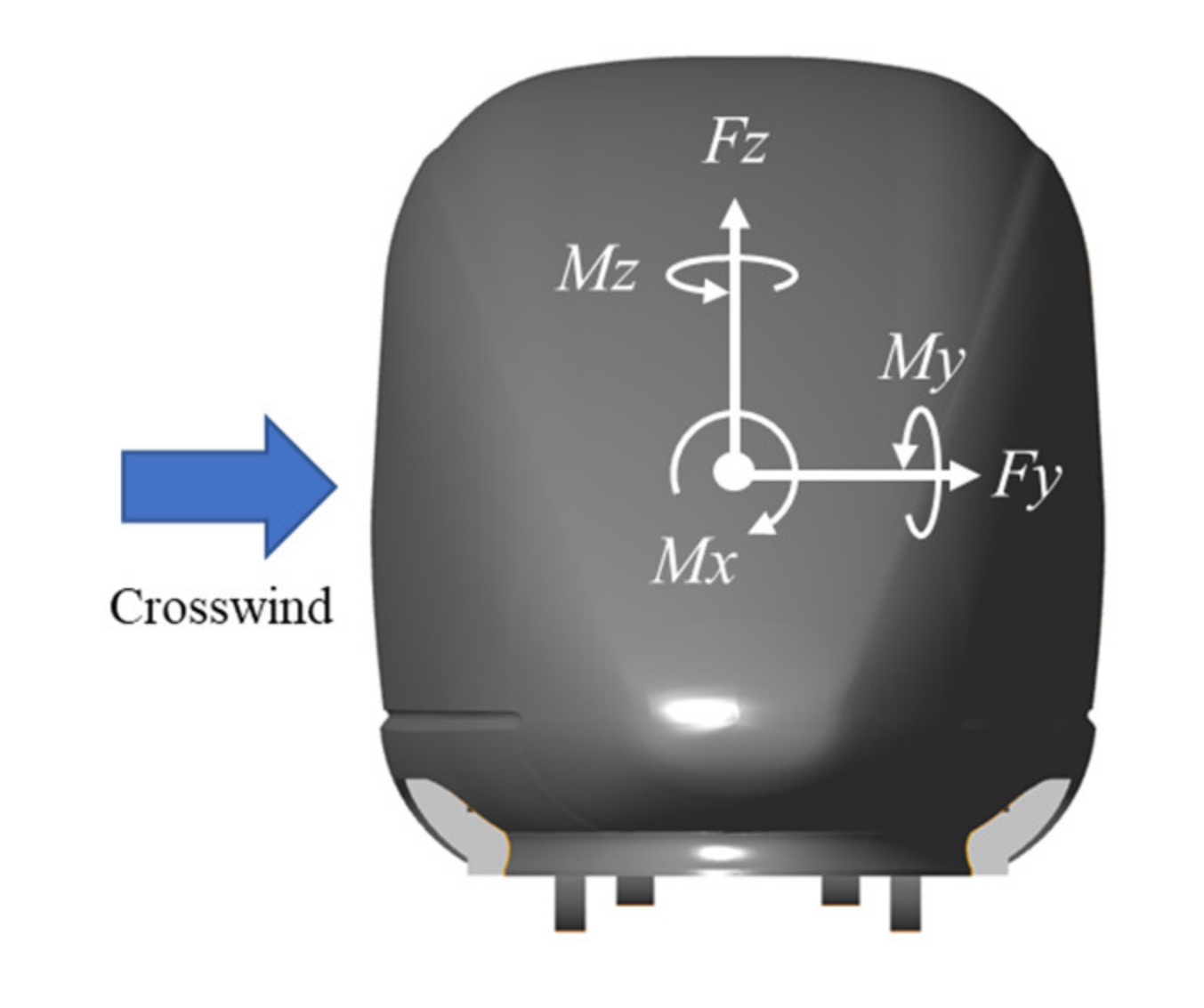
Aerodynamic drag matters to energy consumption while posing a slight risk to train safety, so it was not considered in running safety in the present study. Figure 4 shows the main focus of the current study, the changing characteristics of the lateral force (), lift force (), rolling moment (), pitching moment (), and the yawing moment () of each car were recorded during the train’s rung. Here, the directions of the moment were determined according to the right-hand principle. As shown in Figure 4, the origins of the moment coordinate system were at the center of gravity of each car, and the same motion as the train was assigned to each local coordinate system to capture the moment during its run.
In the present study, the aerodynamic forces and moments were given as a dimensionless form, according to Equations (1)–(5). In Addition, the dimensionless pressure distribution was also employed to show the different flow patterns on the train with and without the posture.
where , , , , , are the side force, lift force, rolling moment, pitching moment, yawing moment of the train, respectively, and , , , , are the corresponding dimensionless coefficients of these aerodynamic indicators. is the pressure coefficient and is the air density and takes a value of 1.225 kg/m3. S is the train’s cross-sectional area (10.84 m2 for this train) and H is the train height, which was introduced in Section 2.1; is the resultant velocity in the domain (85.7 m/s); is the ambient atmospheric pressure; p is the train surface pressure; and H is the height of the train (3.89 m).
3. Validation
3.1. Grid Sensitivity Test
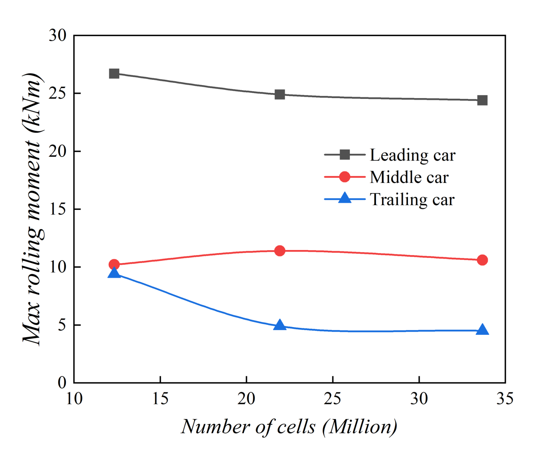
As an essential reference, the maximum rolling moment of the three cars with and without a given posture during the entire traverse through the crosswind region were compared to test the sensitivity of the grid numbers. Here, the velocity of the train was 300 km/h and that of the crosswind was 20 m/s. The results are presented in Figure 5. It can be seen that the coarse mesh could not produce a convergent result, while the medium and fine meshes provided good consistency. Accordingly, the coarse mesh was incapable of predicting the flow field around the train, especially near the tail car. In contrast, the medium mesh showed reasonable results and was, therefore, used in the current simulations.
3.2. Experimental Validation
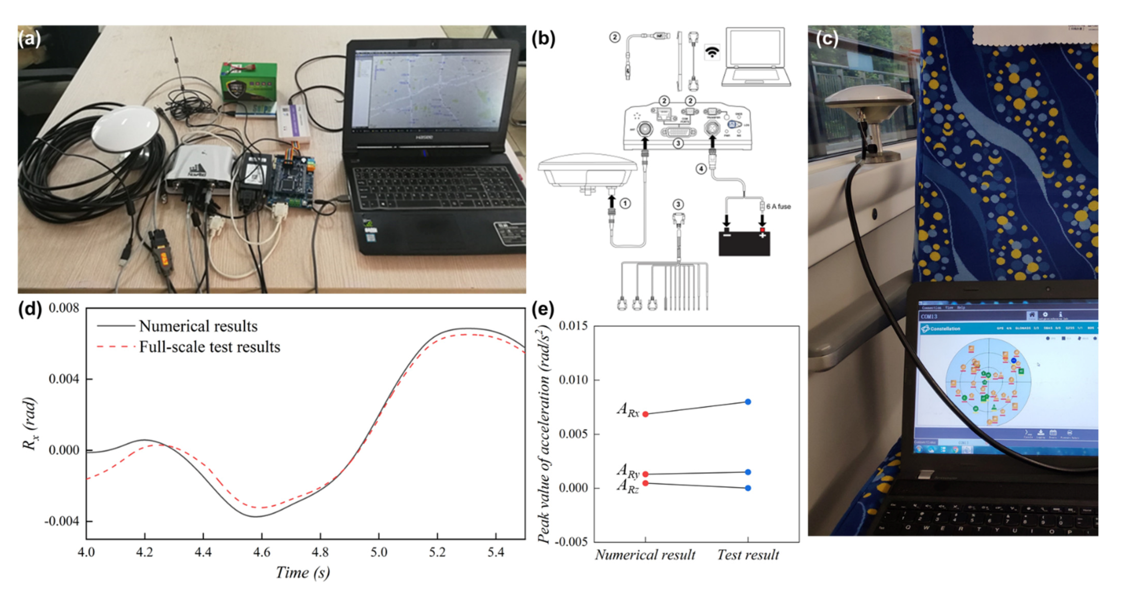
The current numerical method was verified using a full-scale test carried out in a CRH3 train, such as that used in the numerical simulations. As presented in Figure 6a, the PP7-E1 system was used in the test. PP7-E1 is an integrated navigation device developed by NovAtel. The G320 inertial module was added based on the PwrPak7 satellite navigation receiver, using a 7 series SPAN combination algorithm, and were incorporated into the current PP7-E1 (PwrPak7-E1) integrated navigation device. The PP7-E1 device can output real-time positioning and attitude measurement data, as well as more primitive satellite navigation data and inertial data (satellite observations, ephemeris, acceleration, angular rate, etc.). As shown in Figure 6a,b, the entail data acquisition system in the full-scale test included the PP7-E1 receiver, I/O cable, GNSS antenna, antenna cable, PP7 power cable, power supply, and a laptop. During the test, the GNSS antenna-based PP7-E1 test system ensured a time accuracy of 20 ns RMS under the maximum speed limit of 499 m/s and a speed error of less than 0.015 m/s, while an attitude angle error of 0.038° could be obtained after post-processing. In the experiment, a data output frequency of 100 Hz was adopted to ensure that the transient change of the train attitude was well captured. This system was employed to measure the attitude change of the second car of a CRH3 train, as shown in Figure 6c.
Note that this experiment aimed to verify the accuracy of the dynamic response output by the dynamic model results, whose input was obtained from the numerical simulation methods in Section 2.2, Section 2.3 and Section 2.4. That is, the CFD results (the aerodynamic forces and moments) and the dynamic system were not verified individually; instead, the whole process was validated directly using the dynamic response from the experiment, which was not only a challenge to the CFD method but also to the dynamic model. The test was conducted in an environment with almost no wind, so a similar environment between 4 and 5.5 s in the simulation was used for verification. Figure 6d shows a comparison of the test and simulation results of the overturning angle, and Figure 6e shows the difference of the maximum acceleration of , and . Note that the full-scale test results were shown after a filtered processing. It can be seen that the numerical simulation results obtained by using the present methodology in this study were generally in good agreement with the full-scale test. However, there were some obvious differences in the beginning, which could be attributed to the influence of the trailing car suffering the crosswind flow in the numerical simulation, which in turn changed the surrounding flow of the middle car. In addition, the ambient wind speed in the full-scale test could not be kept at 0 as in the numerical simulation, which was also a source of some differences. Nevertheless, the error between the current numerical simulation results and the experimental results is sufficient to guide engineering problems.
4. Results
4.1. Aerodynamic Responses
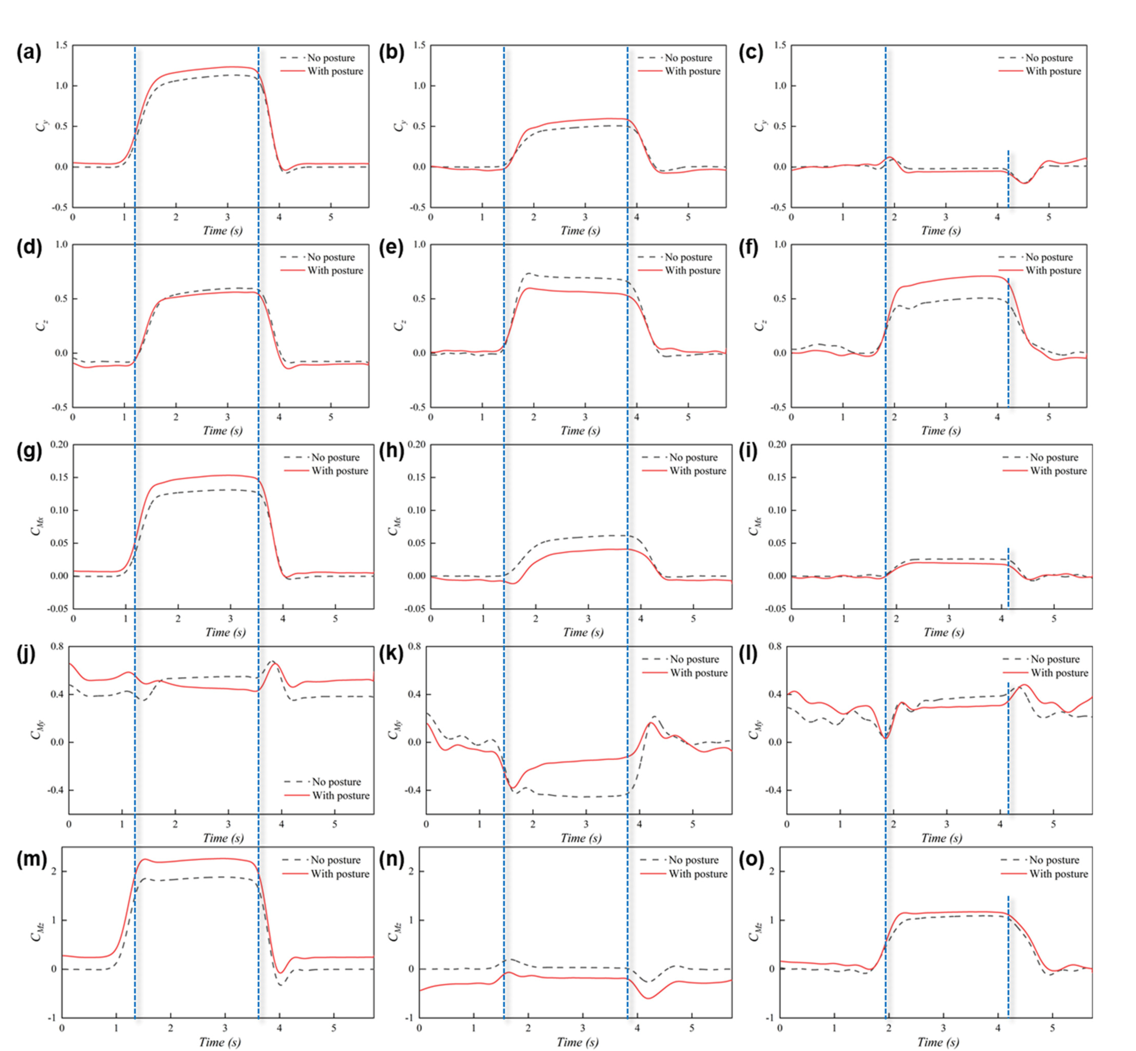
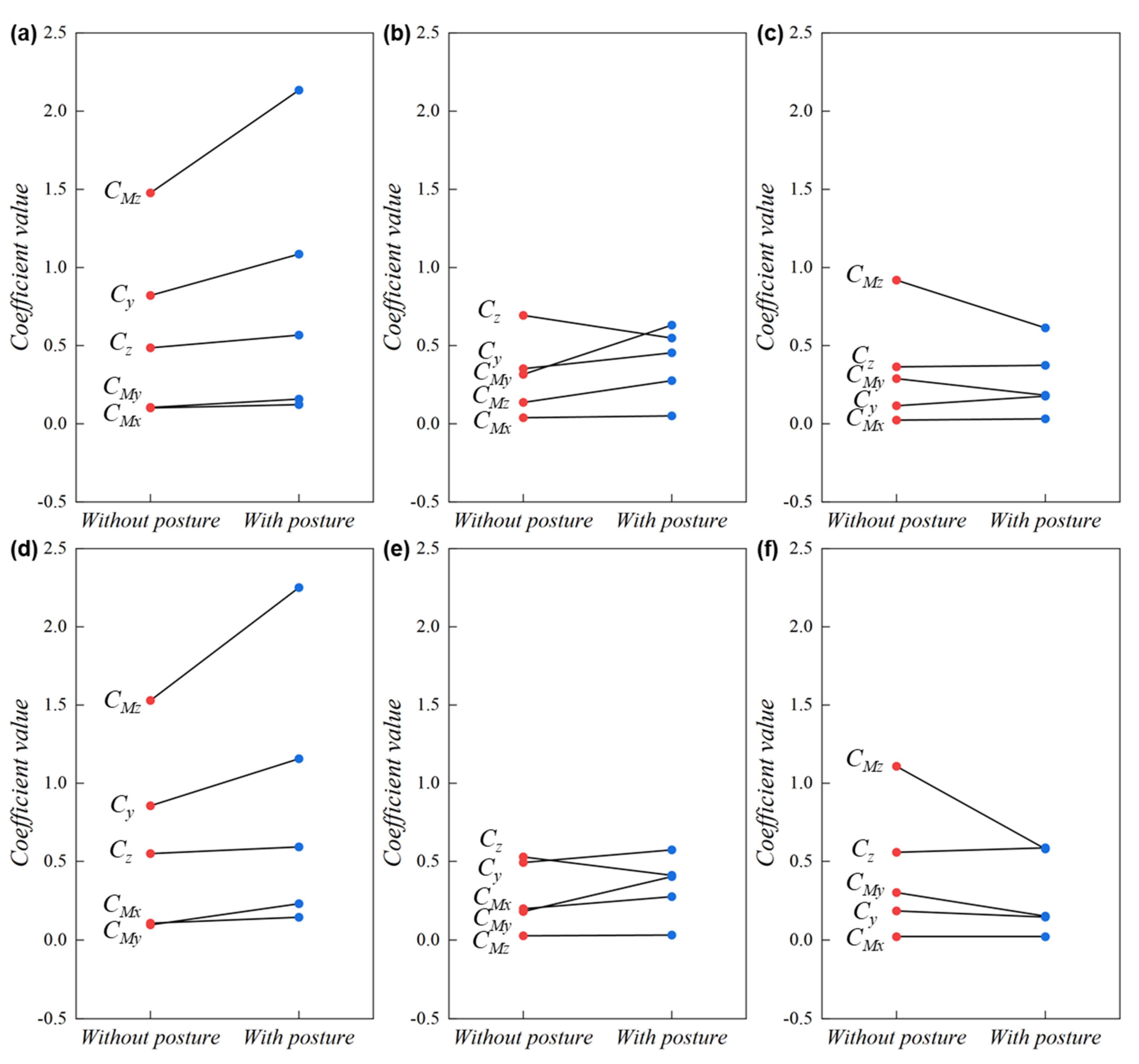
Figure 7 shows the time-varying aerodynamic coefficients of each car during the train’s run, from 100 m before the crosswind region to 100 m after the tail car exits. The speeds of the train and the crosswind were 83.33 m/s and 20 m/s, respectively, giving a yaw angle of 13.5°. The time points when the corresponding car entered and left the crosswind region were given in each figure to explore the transient influence of the crosswind on the aerodynamics of the train. The results of the train with and without the consideration of posture were included in each figure to compare the aerodynamic differences. The range of the coefficient values of the sub-figures was maintained to facilitate the analysis of the different performances among various aerodynamic coefficients. The peak-to-peak value of the aerodynamic coefficients obtained when each car of the train entered and left the crosswind region was also calculated and shown in Table 2 and Figure 8, which quantified the transient fluctuations. The period when each car entered and left the crosswind region was captured—from 0.1 s before the corresponding car started to enter the crosswind region, to 0.1 s after it exited. Based on this, the periods for the leading, middle, and trailing cars entering the crosswind region were 1.100–1.609 s, 1.409–1.913 s, and 1.713–2.223 s, respectively, while the periods for exiting the region were at 3.500–4.010 s, 3.810–4.313 s, and 4.113–4.624 s, respectively.
As can be seen in Figure 7a–c, the aerodynamic side force of different cars showed great differences. The value of received from the head car to the tail car decreased in order. The value of the head car in the crosswind region was increasing, and the growth rate was the fastest when it had just entered this region due to the increase in the blocking area against the crosswind. When the whole head car was in the crosswind region, the growth rate significantly decreased. When it left the crosswind region, the value quickly dropped to 0, which was the same as before entering the region. The posture of the car head was proven to have a global effect on the value of the leading car, whose rotations gave it a higher side force especially in the crosswind region; however, the values during its exit from the crosswind region were almost the same. The same difference was found in the performance of the middle car, where the original car presented a slightly higher value beyond the crosswind region, but showed a lower value when it was within the crosswind region. Due to the development of the longitudinally flowing boundary layers, the intrusion of crosswind on the trailing car was protected to some extent, so that the trailing car gave much slighter fluctuations when it entered and left the crosswind region. From Figure 8, the peak-to-peak transient fluctuations of the value of the separated cars were always higher when the posture was considered, except for when the tail car exited the crosswind region.
There was no noticeable difference in the maximum lift acting on the leading, middle, and trailing cars, which was similar to that coming from the side force. A default posture combination weakened the aerodynamic lift force of the leading and middle cars, while it strengthened that of the tailing car. Additionally, the difference of values between the trains with and without posture increased from the leading car to the trailing car. The peak-to-peak transient fluctuations of the value of the separated cars were similar or slightly lower with a default posture, while that when the leading car entered the crosswind region increased, as can be seen in Figure 8.
As a combined effect of the aerodynamic side and lift forces, the value of acting on different cars passing through the crosswind region presented a similar trend to values, as exhibited in Figure 7g–i. Here, the combination of the side and lift forces shows a different law of overturning moment: a default posture increased the overturning moment of the leading car, while weakened that of the middle and trailing cars. According to Figure 8, is the smallest numerically, all distributed between –0.05 to 0.15, and the peak-to-peak difference is not obvious.
The most significant difference was found in the trend and the value of the pitching moments of different cars. The value of the leading and trailing cars were always positive during the train run, while most of the time, the middle car showed a negative value. As shown in Figure 7j, the difference brought by the posture was not only significantly concentrated in the crosswind area, but the discrepancy of the value was even higher at the region beyond the crosswind, while the posture caused the value of the leading car inside the crosswind region to decrease. An obvious difference can be found in the values when the middle car ran in the crosswind region, where a given posture weakened the negative value that the origin train maintained. Therefore, the peak-to-peak value of the value always had a noticeable difference, although they are relatively and numerically low.
A low yawing moment was found when the middle car passed through the crosswind region, and those of the head and the tail cars changed significantly because they were only connected to other vehicles at one end. The effect brought by the posture on the value was much simpler compared to the other aerodynamic coefficients: this difference law never changed according to the time, and a given posture always made the value of the leading and trailing cars greater, but that of the middle car lower. The peak-to-peak values of were the numerically largest at the leading and trailing cars, and increased at the leading car while decreased at the other cars due to the given posture. It should be noted that the reason why the middle car was obviously different from the head and the tail cars for and values is that it is geometrically symmetrical in the length direction, while the head and tail cars have a strong asymmetric flow due to the presence of streamlined structures so that different time-varying and values were generated.
4.2. Flow Patterns
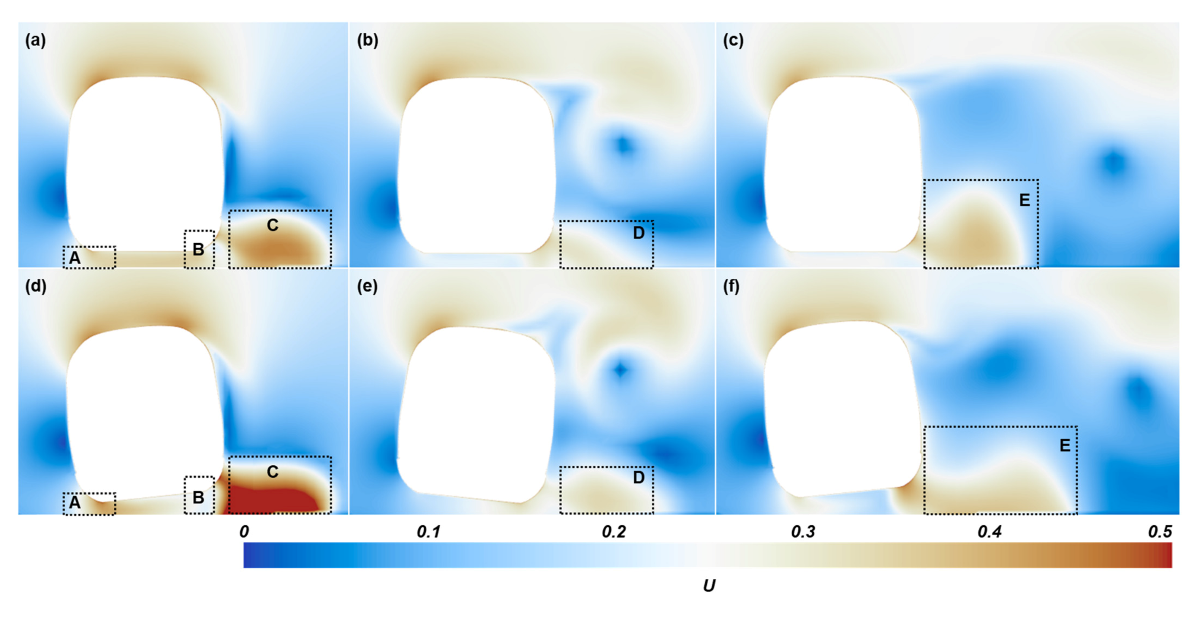
Figure 9 shows the distribution of the dimensionless velocity U the y-z planes at the middle length of the leading, middle, and trailing cars. Here, the value of U can be calculated as:
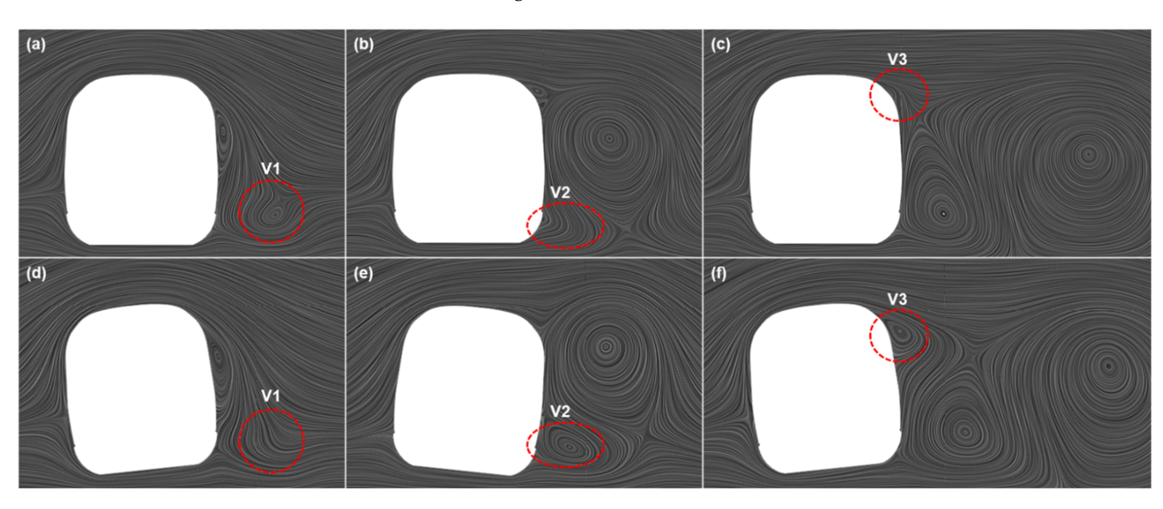
where u is the velocity of the flow in the domain obtained by numerical simulations. This comparison was based on the time when the train arrived in the middle of the crosswind region. Additionally, the velocity vector fields on these planes displayed in the form of line integral convolution are also given, helping to understand these flow structures.
According to Figure 9a,d, the distribution patterns of the velocity field near the leading car were the same: a local high-speed flow was formed at the top and bottom of the vehicle, and a much higher-speed flow could be seen in the area near the ground downstream of the leading car. Due to an overturning posture, the entrance of the crosswind into the underbody of the vehicle shrunk, resulting in greater underbody flow, as seen in region A. On the contrary, the exit of the escaping flow from the bottom of the vehicle was larger due to the existence of this overturning posture, making the flow in area B greater, thus creating the low-speed area. In area C, an obvious vortex (V1 in Figure 10) was generated at the leeward side of the original leading car, but no obvious swirling flow was found behind the train with posture. This is the reason for the difference in velocity flow in this area. Around the middle car, as shown in Figure 9b,e, most of the flow fields around the vehicle body are similar, only the D area (the same as the C area in Figure 9a,d) produced a different shape for the high-speed area, which is attributed to the additional vortex (V2 in Figure 10) generated by the shrunk exit of the underbody flow of the middle car with posture. The overturning posture of the trailing car not only caused the roof airflow to form a stronger flow separation (V3 in Figure 10) on the leeward side of the vehicle, but also a main large-scale vortex structure on the backward side.
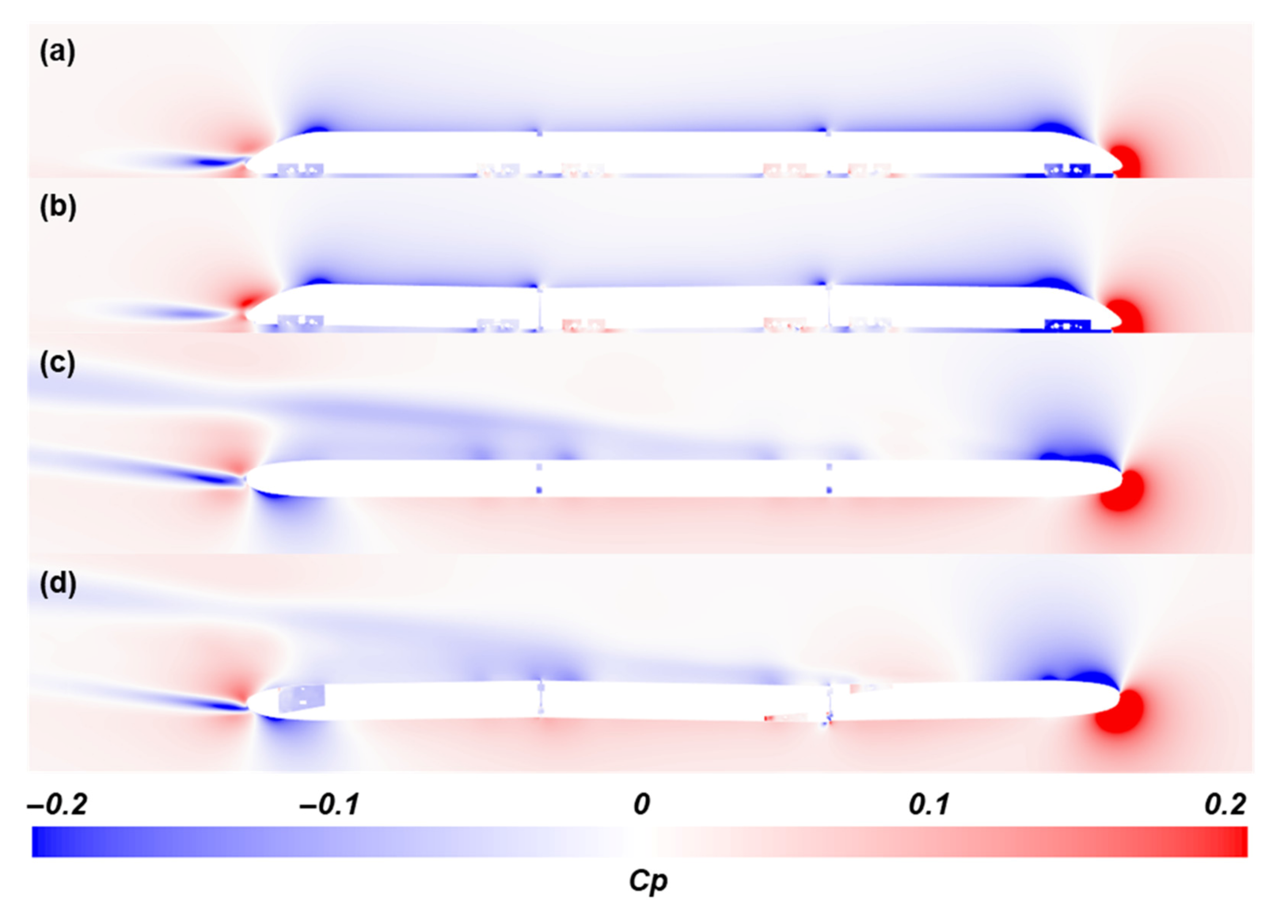
Figure 11 shows the pressure distribution on the longitudinal and horizontal planes around the two trains to understand the difference in flow patterns along the train length. The longitudinal plane was located at y = 0 m, and the horizontal plane was located at z = 1.5 m. From Figure 11a,b, the pressure distribution on the symmetry plane of the train was almost unaffected by the posture change, and only the near-wake area had a relatively obvious difference, where the streamlined structure of the trailing car of the train with posture bore large positive pressure, and smaller negative pressure was found in the center of the wake plume flow. An even smaller difference was found in the pressure distribution pattern on the horizontal plane, seen in Figure 11c,d. Since different postures were applied to separated cars, there were quite local and slight differences due to geometric discontinuities at the car joints.
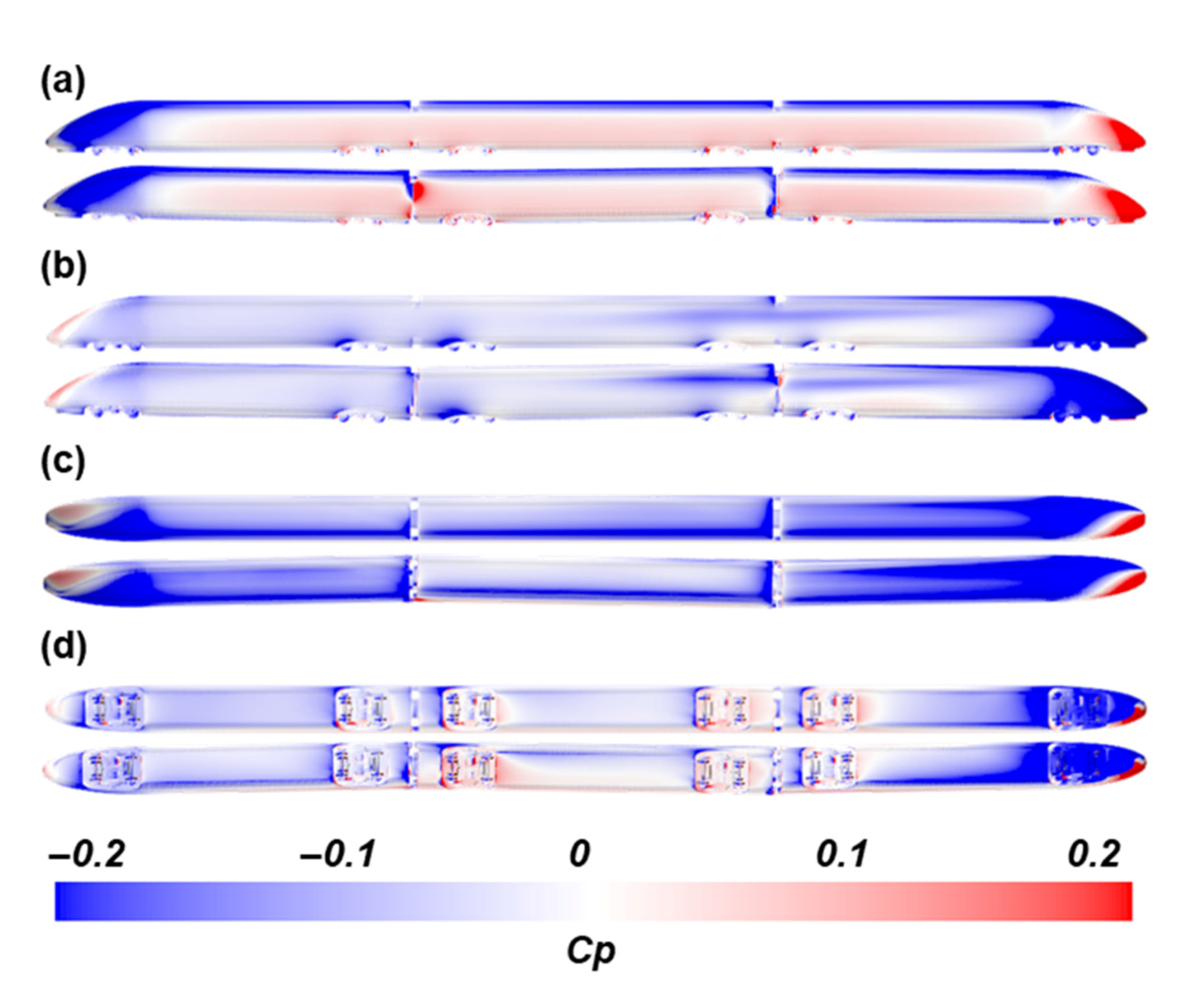
Figure 12 presents the surface pressure distribution of the train with and without the posture when it was located in the same position as Figure 9, Figure 10 and Figure 11 from four different perspectives. Similar to the findings in Figure 11, no significant differences in pressure distribution patterns were found on different surfaces of the train, such as the accumulation of positive pressure on the nose tip of the leading car and the accumulation of negative pressure on the nose tip of the trailing car. The pressure difference was mainly reflected on the edge structure of the vehicle, such as the transition area between the side surface and the top surface, the transition area between the side surface and the bottom surface, and the connection of different vehicles. The pressure difference on the edge area of the vehicle is due to the flow difference guided by different train postures, and that of the connection of vehicles resulted from the flow stagnation or separation caused by geometric dislocation.
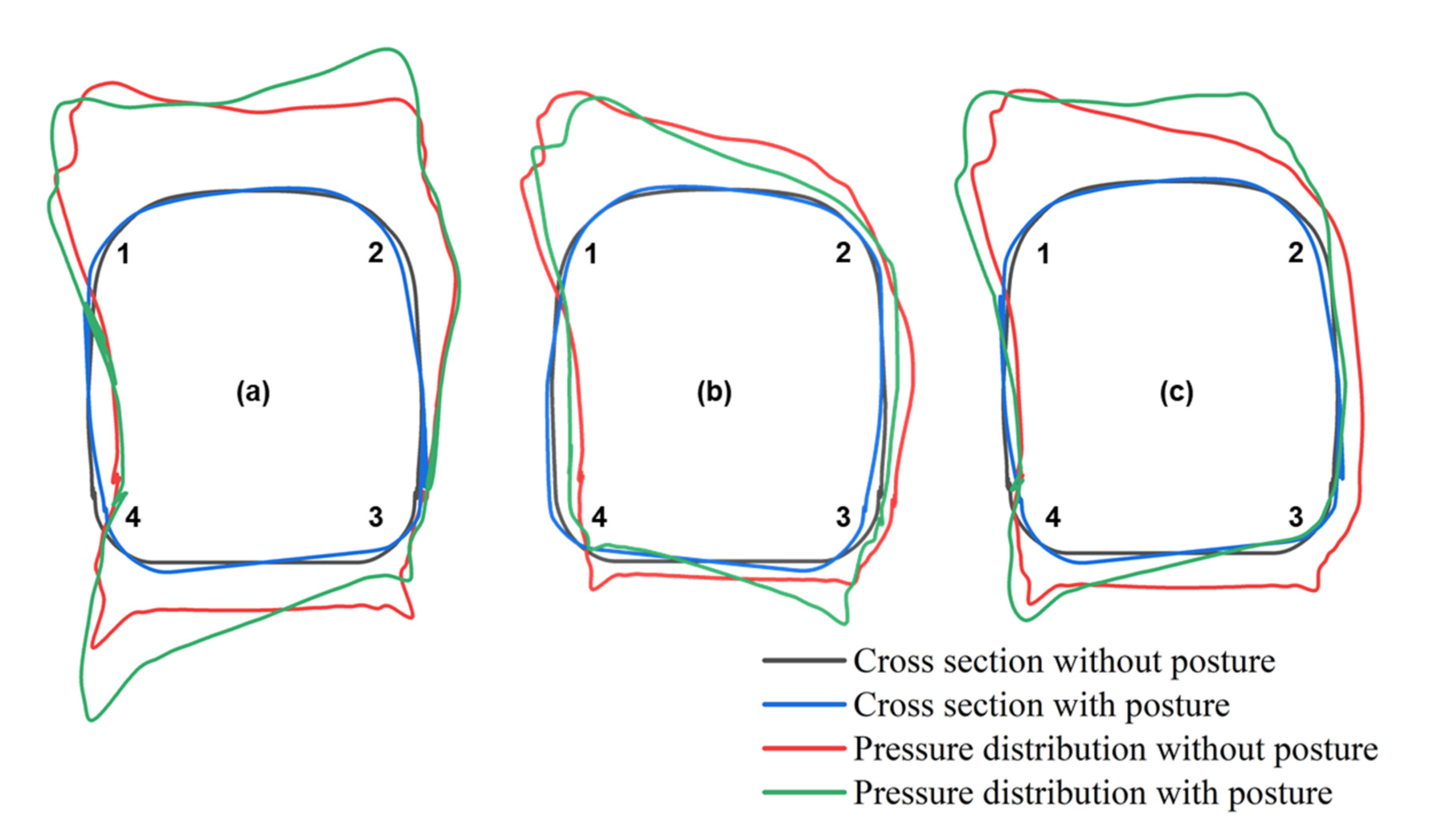
To obtain further quantitative difference in pressure distribution from the distribution pattern in Figure 12, the profiles of the value on the same cross-section as in Figure 9 and Figure 10 are given in Figure 13. The top of the train body often distributed the greatest pressure value, but the largest pressure difference appeared at the junction between the train surfaces. Regardless of whether it is the leading car, middle car, or the trailing car, a general rule can be drawn: the corner where the flow tends to be accelerated instead of being blocked will produce lower pressure than the original situation, as shown in corner 2 and corner 4 in Figure 13b, as well as corner 3 in Figure 13a; when the posture tends to block the airflow, greater pressure will be formed, such as in corner 4 in Figure 13a and corner 3 in Figure 13b. In addition, there was almost no difference in the pressure generated on the windward and leeward sides of the leading car in different postures, though this difference gradually became larger with the development of the longitudinal airflow, which was prominent on the leeward side of the trailing car.
4.3. Running Safety
The transient aerodynamic load of the running train was inputted into the train-track coupled dynamic model to conduct a dynamic analysis of the running safety. The coupled model consists of three sub-models: train subsystem, track subsystem, and wheel–rail contact model. Every train carriage is modelled as a set of seven rigid bodies, including one carriage body, two bogies, four wheelsets, and bottom and top suspensions, without taking into account the longitudinal interaction between carriages. The track structure subsystem’s 3D model must be created using the finite element approach. The spring-damper unit simulates the rubber pad between the rail and the rail slab, and the track slab is regarded as totally fixed. Track irregularity, which includes vertical, directional, level, and gauge irregularity, is a major cause of train vibration interference. The geometry contact relationship between wheel and rail is solved using the 3D space trace approach. For the sake of simplicity, the current study did not describe the dynamic system model specifically, which can be seen in Deng’s research [23]. According to the previous studies, the leading car was generally exposed to higher running safety risks than the middle and trailing cars due to much more terrible aerodynamic fluctuations. However, considering the influence of posture, whether this is still correct or not is unknown. Therefore, the running safety of all cars were given and analyzed here, which means studying the effect of the given posture on DC, WLRR, and the posture changes of the train.
4.3.1. Derailment Coefficient
The derailment coefficient of the train can be calculated by the contact force of the wheels according to the TB10621-2009 standard, which is given as:
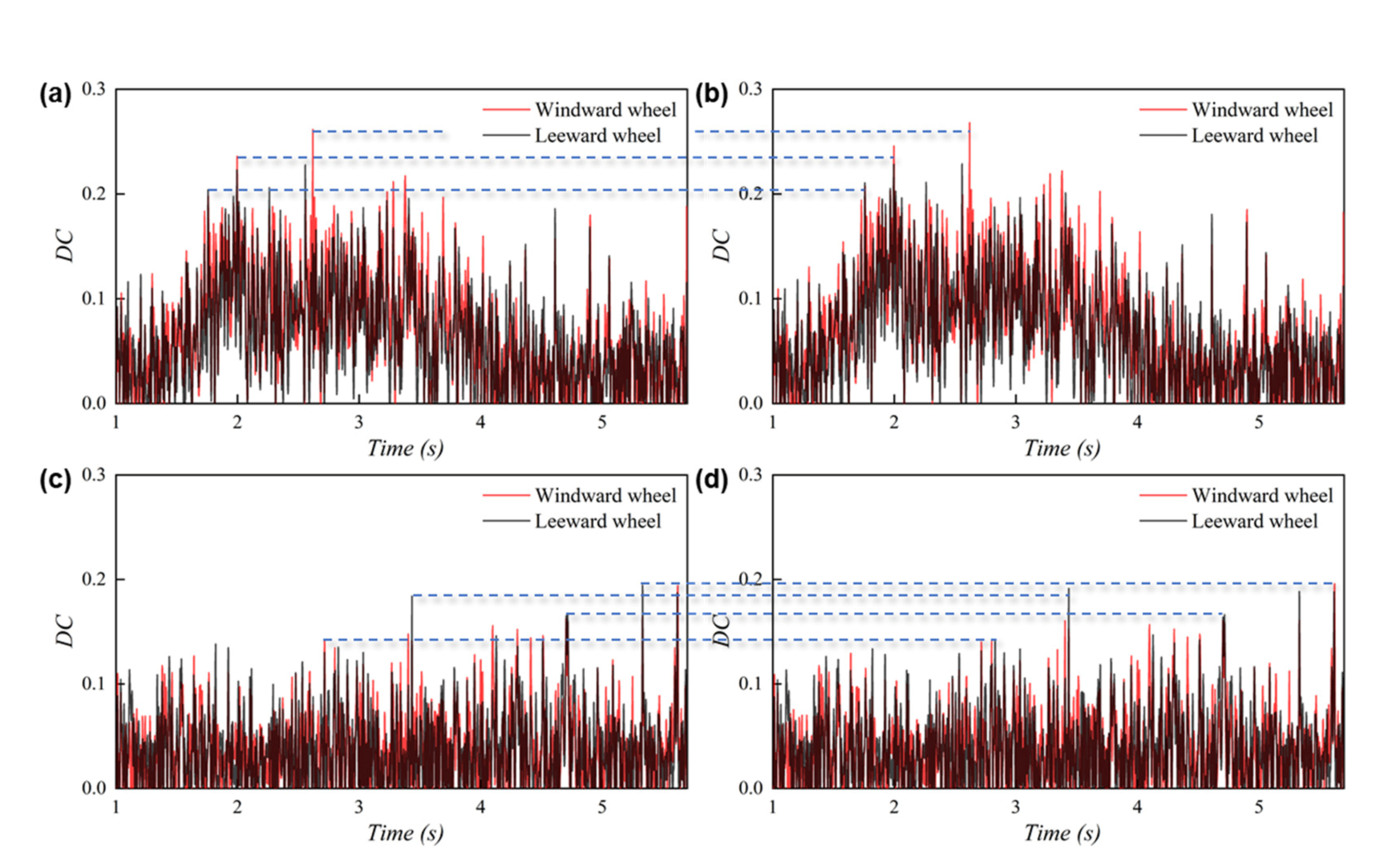
where Q and P are the lateral and vertical forces acting on the wheels, respectively. Figure 14 shows the time-varying DC values of the first wheelset of the leading car and the last wheelset of the trailing car of the train, with and without the given posture.
As trains passed the crosswind region, the DC values on these two wheelsets showed different performances. After the first wheelset of the leading car entered the crosswind region, the DC value began to rise and fluctuated at a high level. When it left the crosswind region at about t = 4 s, the value of DC began to fall. The highest value appeared at about t = 2.6 s. As shown in Figure 14b, the DC development trend of the train with and without the designated posture over time was the same, but the consideration of posture gave a larger peak value, which meant that the safety situation of the train with posture was highly threatened. For the trailing car, same as the lateral force performance in Figure 7c, the fully developed boundary layer weakened the impact of the crosswind to a certain extent, resulting in a significant reduction of difference of the DC value of two different trains. The trailing car of the train with posture only produced a slightly higher global sub-peak value than that of the train without posture when the time was at about 3.4 s, and there was no significant difference at the other time.
4.3.2. Wheel Load Reduction Rate
When a train runs at a high speed, the wheels do not stay horizontal but move up and down due to the vibration, and the wheel weight of the wheelset increase or decrease. Even if the lateral force on the side of the reduced wheel weight is small (or even none), there may be lateral relative displacement with the wheels, which leads to a derailment. Hence, the WLRR was also considered in the evaluation of the running safety in terms of:
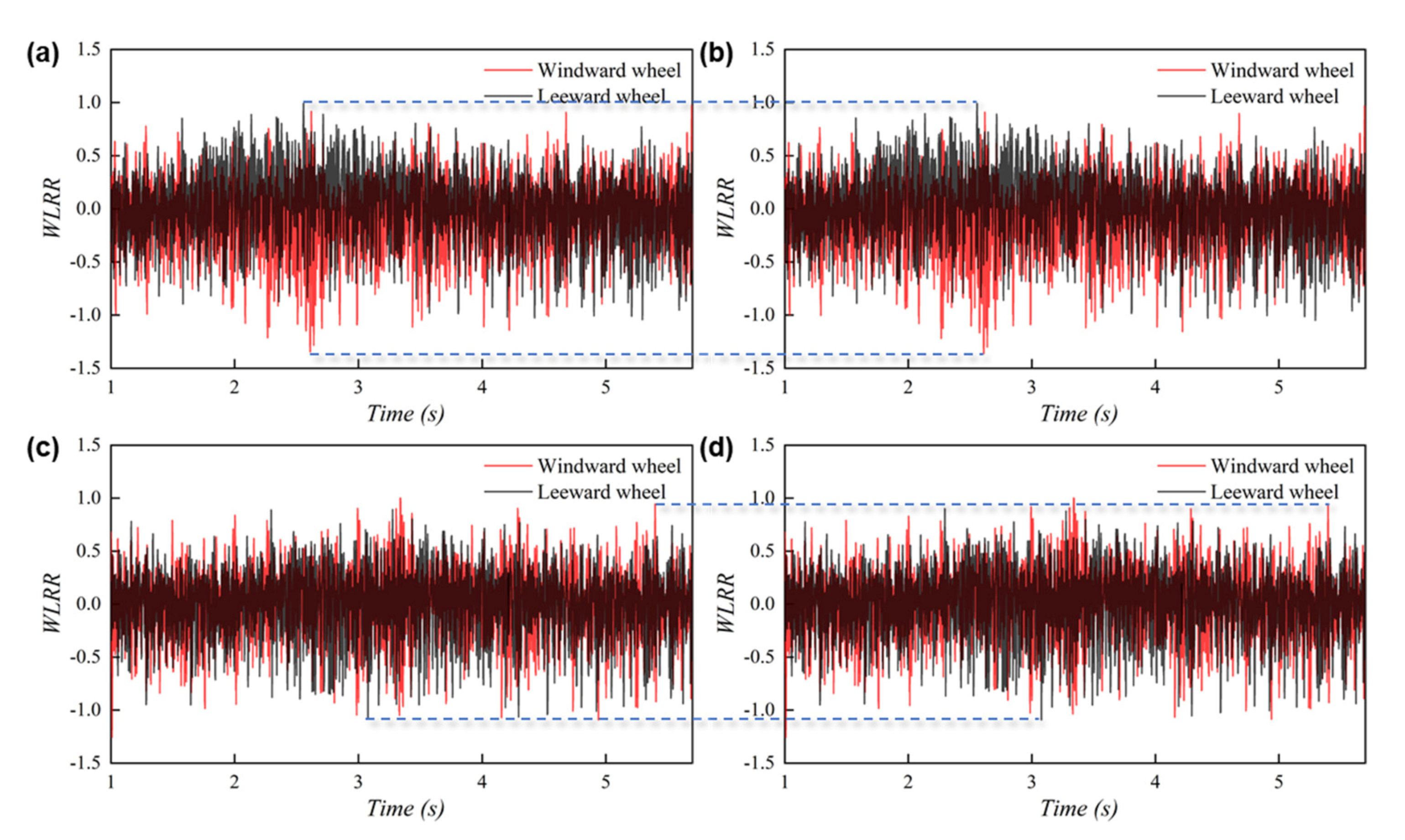
where ΔP is the load reduction in the wheel load, P is the average static wheel load of the wheelset, and is the maximum overrun duration. The same as Figure 14, Figure 15 shows the time-varying WLRR values of the first wheelset of the leading car and the last wheelset of the trailing car of the train, with and without the given posture. According to the definition of WLRR, its theoretical maximum value is +1, which means that the wheel–rail contact force is 0 and the wheel–rail disengagement state is at this time, so the maximum value of WLRR cannot exceed 1. However, its lowest value is not −1. In the process of high-speed train operation, if there is irregularity on the rail surface (the rail surface is slightly arched upwards) or a transient aerodynamic impact at a certain moment. The wheels will have a transient impact on the rail, where the impact force can even reach several times the static wheel weight, which is why WLRR can reach a value higher than −1.
No remarkable difference in the WLRR value could be found when the train with and without a designed posture passed the crosswind region. Their distributions, peak values, and the developing mode were all the same, saying that a slightly given posture cannot significantly influence the performance of WLRR.
4.3.3. Running Posture
Furthermore, the coupled dynamic system provides the posture changes of the train passing through the crosswind region with and without the given posture. The running posture is a part of the safety analysis and was studied by a previous study [26], while only the posture of the leading vehicle was investigated. In the present study, the posture changes of the leading, middle, and trailing cars of the trains with and without the initial posture in five degrees of freedom (lateral and vertical displacement and rotation in three directions) were compared and analyzed.
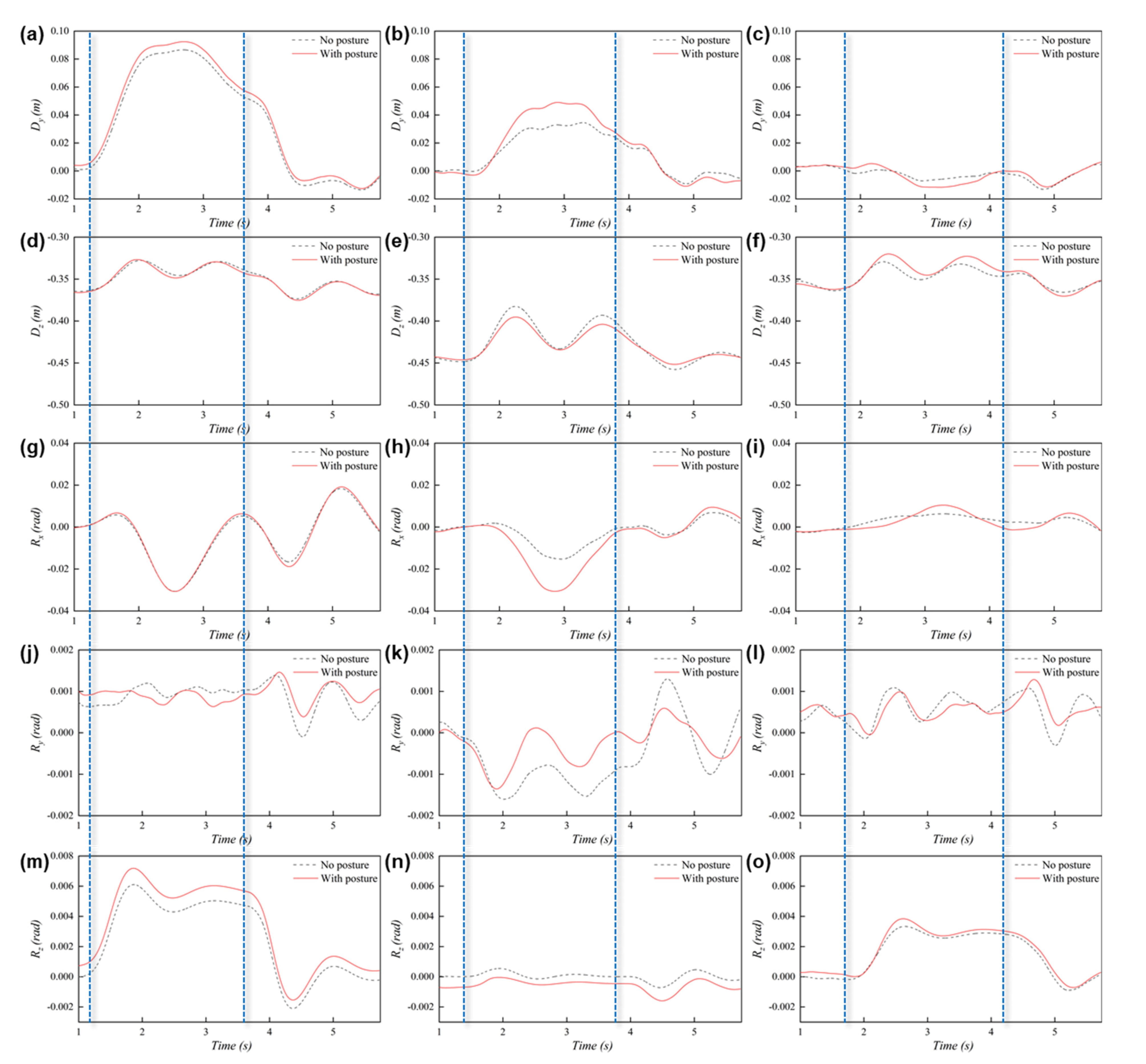
Figure 16 shows the changes of different degrees of freedom indexes when the train passed the crosswind region with regard to two different initial postures. In the figure, Dy, Dz, Rx, Ry, Rz are the lateral and vertical displacements (unit: m) and the rotation of the x, y, and z axes (unit: rad). The diagram of the running posture of the train is also given in each figure, where the transparent one represents the original position, and another is the posture caused by the crosswind. The same range of the y axis was kept constant for a single degree of freedom to understand the different performances of separated cars.
According to Figure 16a–c, there were obvious differences in the displacement characteristics of the three cars in the lateral direction, and the magnitude of the displacement decreased from the leading car to the trailing car, which could be attributed to the differences in their lateral forces, as described in Figure 7a–c. In addition, the influence of the given posture on the lateral displacement of the train is consistent with the law of lateral force: the preset posture tended to push the leading car and the middle car further in the direction of the crosswind; while the lateral displacement of the trailing car that did not consider the posture in the crosswind area fluctuated slightly around 0, and that of the trailing car with posture increased, whether same or opposite to the direction of the crosswind. From Figure 16d–f, all three cars had downward vertical displacements, and they all showed two humps with similar peak values within the crosswind region. Only a slight difference can be found in the leading car, while relatively larger differences were formed in the vertical displacement of the middle and the trailing cars. For the overturning angle shown in Figure 16g,i, due to the similarity of the preset attitude on the lateral and vertical displacements of the leading car (see Figure 16a,d), the overturning angles shown by the two leading cars were almost the same, but the middle car was different: the middle car with posture was found to have a reverse overturning trend much larger than the original car. The overturning rotation of the trailing car was similar to the change in lateral displacement (see Figure 16c). The pitching rotation changes of the three cars were the most active, and the difference caused by the preset posture was not limited to the crosswind region. The most obvious difference was also found in the middle car: the preset posture reduced the pitching angle not only inside but also beyond the crosswind region to around 0. For the leading and trailing vehicles with a streamlined structure, the preset posture slightly increased their maximum values. As shown in Figure 16m–o, the influence of a given posture on the yawing angle is clear and simple, which made the positive yawing rotation of the leading and trailing cars larger and increased the negative yawing rotation of the middle car in reverse.
4.3.4. Safety Domain
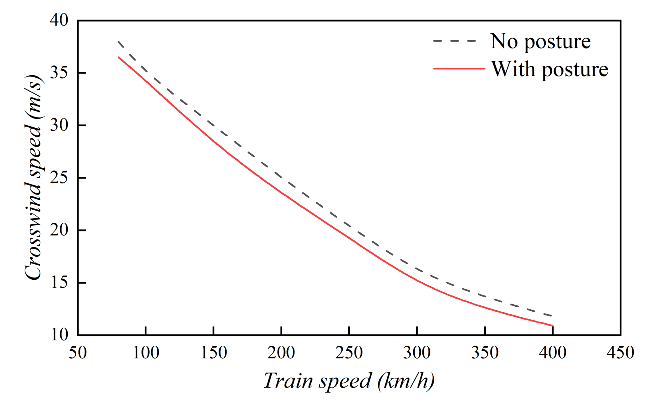
Analyses of critical speeds of trains traveling in various crosswinds define the safety domain of trains running in a crosswind with attitude change taken into account. In the present study, the values of DC and WLRR are employed as the running safety indices, based on which Figure 17 shows the running safety domain in terms of the relationship between the speed of crosswind and train. A train’s critical speed is higher when there is a weaker crosswind, and it is lower when there is a stronger crosswind. The train’s ability to overcome crosswind decreases as it speeds up. With the consideration of posture, a train is proven to withstand a weaker crosswind. As a result, for high-speed and super-speed trains, extra attention should be given to the wind environment.
5. Conclusions
The URANS turbulence model was employed to calculate the time-varying aerodynamic forces and moments of the train with and without a preset posture as it passes through a crosswind region. Based on the different characteristics of the train derailment coefficient and wheel load reduction rate, the effect of each car’s preset posture on running safety was also investigated. The transient changes of the running posture of each car of the train with and without the designed posture were also compared and analyzed in five degrees of freedom. The main conclusions can be drawn as follows:
- The original posture provided significant changes to the train’s aerodynamic coefficients. Various effects and laws of the aerodynamic coefficients were found at different separated cars. These discrepancies can be attributed to the different flow patterns such as the pressure distribution and vortex structure around the trains with and without present posture. Obvious fluctuations exist in the aerodynamic coefficients when the train enters and exits the wind barrier.
- A slightly larger maximum derailment coefficient was found on the first bogie of the leading car with a preset posture. This difference in the trailing car was not as obvious as that of the leading car. The development law as well as the maximum and minimum values of wheel load reduction rate hardly changed with the preset attitude. The maximum values of these two indicators of the leading car were higher than those of the trailing car, indicating that the leading vehicle has greater running safety risks.
- There were obvious differences in the displacement characteristics of the three cars in the lateral direction and the rolling rotation, and the magnitude of the posture changes decreased from the leading car to the trailing car. The pitching rotation changes of the three cars were the most active, and the difference caused by the preset posture was not limited to the crosswind region. The influence of a given posture on the yawing angle is clear and simple, which made the positive yawing rotation of the leading and trailing cars larger and increased the negative yawing rotation of the middle car in reverse.
- A train’s critical speed is higher when there is a weaker crosswind, and it is lower when there is a stronger crosswind. The train’s ability to overcome crosswind decreases as it speeds up. The train with the consideration of posture is proven to withstand weaker crosswind.
- Further work may lie in the reproduction of the time-varying posture modifications based on the Dynamic Fluid Body Interaction (DFBI) technique.
Author Contributions
Conceptualization, J.Y. and T.C.; methodology, E.D.; software, E.D.; validation, S.C.; formal analysis, S.C.; investigation, S.C.; resources, W.Y.; data curation, J.Y.; writing—original draft preparation, J.Y.; writing—review and editing, S.G. and Z.G.; visualization, J.Y.; supervision, T.C.; project administration, T.C.; funding acquisition, W.Y. All authors have read and agreed to the published version of the manuscript.
Funding
This research was funded by the National Natural Science Foundation of China (Grant No. 51978670).
Institutional Review Board Statement
Not applicable.
Informed Consent Statement
Not applicable.
Data Availability Statement
Not applicable.
Acknowledgments
The authors acknowledge the computing resources provided by the High-Performance Computing Center of Central South University.
Conflicts of Interest
The authors declare no conflict of interest.
References
- Cheli, F.; Corradi, R.; Tomasini, G. Crosswind action on rail vehicles: A methodology for the estimation of the characteristic wind curves. J. Wind Eng. Ind. Aerodyn. 2012, 104–106, 248–255. [Google Scholar] [CrossRef]
- Baker, C.; Cheli, F.; Orellano, A.; Paradot, N.; Proppe, C.; Rocchi, D. Cross-wind effects on road and rail vehicles. Veh. Syst. Dyn. 2009, 47, 983–1022. [Google Scholar] [CrossRef]
- Cui, T. Study on Fluid-Solid Coupling Vibration and Running Safety of High-Speed Trains. Ph.D. Thesis, Southwest Jiaotong University, Sichuan, China, 2011. (In Chinese). [Google Scholar]
- Zhou, D.; Tian, H.Q.; Lu, Z.J. Influence of strong crosswind on aerodynamic performance of passenger train running on embankment. J. Traffic Transp. Eng. 2007, 7, 6–9. [Google Scholar]
- Liu, Q.K.; Du, Y.L.; Qiao, F.G. Train crosswind and strong wind countermeasure research in Japan. J. China Railw. Soc. 2008, 30, 82–88. [Google Scholar]
- Johnson, T. Strong wind effects on railway operations-16th October 1987. J. Wind Eng. Ind. Aerodyn. 1996, 60, 251–266. [Google Scholar] [CrossRef]
- Branch, R.A.I. Detachment of Containers from Freight Wagons near Cheddington and Hardendale 1 March 2008. Investig. Rep. 2009, 12. Available online: https://www.gov.uk/raib-reports/detachment-of-containers-from-freight-wagons-near-cheddington-and-hardendale (accessed on 20 May 2021).
- Soper, D.; Baker, C.; Sterling, M. An experimental investigation to assess the influence of container loading configuration on the effects of a crosswind on a container freight train. J. Wind Eng. Ind. Aerodyn. 2015, 145, 304–317. [Google Scholar] [CrossRef]
- True, H. Vehicle-Track Coupled Dynamics. Veh. Syst. Dyn. 2020, 1–3. [Google Scholar] [CrossRef]
- Song, Y.; Wang, Z.; Liu, Z.; Wang, R. A spatial coupling model to study dynamic performance of pantograph-catenary with vehicle-track excitation. Mech. Syst. Signal Process. 2021, 151, 107336. [Google Scholar] [CrossRef]
- Deng, E.; Yang, W.; He, X.; Zhu, Z.; Wang, H.; Wang, Y.; Wang, A.; Zhou, L. Aerodynamic response of high-speed trains under crosswind in a bridge-tunnel section with or without a wind barrier. J. Wind Eng. Ind. Aerodyn. 2021, 210. [Google Scholar] [CrossRef]
- Chen, Z.; Liu, T.; Li, W.; Guo, Z.; Xia, Y. Aerodynamic performance and dynamic behaviors of a train passing through an elongated hillock region beside a windbreak under crosswinds and corresponding flow mitigation measures. J. Wind Eng. Ind. Aerodyn. 2021, 208. [Google Scholar] [CrossRef]
- Montenegro, P.A.; Heleno, R.; Carvalho, H.; Calçada, R.; Baker, C.J. A comparative study on the running safety of trains subjected to crosswinds simulated with different wind models. J. Wind Eng. Ind. Aerodyn. 2020, 207. [Google Scholar] [CrossRef]
- Richardsona, G.M.; Richards, P.J. Full-scale measurements of the effect of a porous windbreak on wind spectra. J. Wind Eng. Ind. Aerodyn. 1995, 54–55, 611–619. [Google Scholar] [CrossRef]
- Hashmi, S.A.; Hemida, H.; Soper, D. Wind tunnel testing on a train model subjected to crosswinds with different windbreak walls. J. Wind Eng. Ind. Aerodyn. 2019, 195, 104013. [Google Scholar] [CrossRef]
- Tomasini, G.; Giappino, S.; Cheli, F.; Schito, P. Windbreaks for railway lines: Wind tunnel experimental tests. Proc. Inst. Mech. Eng. Part F J. Rail Rapid Transit. 2016, 230, 1270–1282. [Google Scholar] [CrossRef] [Green Version]
- Chu, C.R.; Chang, C.Y.; Huang, C.J.; Wu, T.R.; Wang, C.Y.; Liu, M.Y. Windbreak protection for road vehicles against crosswind. J. Wind Eng. Ind. Aerodyn. 2013, 116, 61–69. [Google Scholar] [CrossRef]
- Guo, Z.; Liu, T.; Chen, Z.; Xia, Y.; Li, W.; Li, L. Aerodynamic influences of bogie’s geometric complexity on high-speed trains under crosswind. J. Wind Eng. Ind. Aerodyn. 2020, 196, 104053. [Google Scholar] [CrossRef]
- Guo, Z.; Liu, T.; Chen, Z.; Liu, Z.; Monzer, A.; Sheridan, J. Study of the flow around railway embankment of different heights with and without trains. J. Wind Eng. Ind. Aerodyn. 2020, 202, 104203. [Google Scholar] [CrossRef]
- Niu, J.; Wang, Y.; Liu, F.; Chen, Z. Comparative study on the effect of aerodynamic braking plates mounted at the inter-carriage region of a high-speed train with pantograph and air-conditioning unit for enhanced braking. J. Wind Eng. Ind. Aerodyn. 2020, 206, 104360. [Google Scholar] [CrossRef]
- Zhai, Y.; Niu, J.; Wang, Y.; Liu, F.; Li, R. Unsteady flow and aerodynamic behavior of high-speed train braking plates with and without crosswinds. J. Wind Eng. Ind. Aerodyn. 2020, 206, 104309. [Google Scholar] [CrossRef]
- Yang, W.; Deng, E.; Zhu, Z.; He, X.; Wang, Y. Deterioration of dynamic response during high-speed train travelling in tunnel–bridge–tunnel scenario under crosswinds. Tunn. Undergr. Sp. Technol. 2020, 106, 103627. [Google Scholar] [CrossRef]
- Deng, E.; Yang, W.; Lei, M.; Zhu, Z.; Zhang, P. Aerodynamic loads and traffic safety of high-speed trains when passing through two windproof facilities under crosswind: A comparative study. Eng. Struct. 2019, 188, 320–339. [Google Scholar] [CrossRef]
- Baker, C.J.; Jones, J.; Lopez-Calleja, F.; Munday, J. Measurements of the cross wind forces on trains. J. Wind Eng. Ind. Aerodyn. 2004, 92, 547–563. [Google Scholar] [CrossRef]
- Cui, T.; Zhang, W.; Sun, B. Investigation of train safety domain in cross wind in respect of attitude change. J. Wind Eng. Ind. Aerodyn. 2014, 130, 75–87. [Google Scholar] [CrossRef]
- Yan, J.; Chen, T.; Deng, E.; Yang, W.; Cheng, S.; Zhang, B. Aerodynamic Response and Running Posture Analysis When the Train Passes a Crosswind Region on a Bridge. Appl. Sci. 2021, 11, 4126. [Google Scholar] [CrossRef]
Figure 1.
Geometric models employed in the numerical simulation: (a) the realistic CRH3 train; (b) the CAD model train; (c) front view of the train; (d) length components of the train; (e) train model with specific posture, according to Table 1.
Figure 1.
Geometric models employed in the numerical simulation: (a) the realistic CRH3 train; (b) the CAD model train; (c) front view of the train; (d) length components of the train; (e) train model with specific posture, according to Table 1.

Figure 2.
Computational domain and boundary conditions: (a) overall side view; (b) side view of the overset region; (c) front view of the computational domain; (d) front view of the overset region.
Figure 2.
Computational domain and boundary conditions: (a) overall side view; (b) side view of the overset region; (c) front view of the computational domain; (d) front view of the overset region.

Figure 3.
Computational mesh employed in the simulations: (a) front view of mesh density in the computational domain; (b) side view of mesh density in the computational domain; (c) mesh distribution around the bogie; (d) the prism layer cells attached to the train surface.
Figure 3.
Computational mesh employed in the simulations: (a) front view of mesh density in the computational domain; (b) side view of mesh density in the computational domain; (c) mesh distribution around the bogie; (d) the prism layer cells attached to the train surface.

Figure 4.
The parameter definition and the origin of the moment coordinate system.

Figure 5.
Maximum rolling moment of three cars predicted by different meshes (in = 300 km/h; = 20 m/s).
Figure 5.
Maximum rolling moment of three cars predicted by different meshes (in = 300 km/h; = 20 m/s).

Figure 6.
The validation of the numerical method: (a) the entire PP7-E1 system; (b) the schematic diagram of PP7-E1 system; (c) the measuring setup in the car; (d) the rolling rotation obtained by numerical simulation and test; (e) the maximum value of the rotation acceleration obtained by numerical simulation and test.

Figure 7.
The time-varying aerodynamic coefficients of each car passing the crosswind with and without posture: (a) of the leading car; (b) of the middle car; (c) of the trailing car; (d) of the leading car; (e) of the middle car; (f) of the trailing car; (g) of the leading car; (h) of the middle car; (i) of the trailing car; (j) of the leading car; (k) of the middle car; (l) of the trailing car; (m) of the leading car; (n) of the middle car; (o) of the trailing car.

Figure 8.
Peak-to-peak values of the aerodynamic coefficients when each car entered and left the crosswind region with and without posture.: (a) entry of leading car; (b) entry of middle car; (c) entry of trailing car; (d) exit of leading car; (e) exit of middle car; (f) exit of trailing car.
Figure 8.
Peak-to-peak values of the aerodynamic coefficients when each car entered and left the crosswind region with and without posture.: (a) entry of leading car; (b) entry of middle car; (c) entry of trailing car; (d) exit of leading car; (e) exit of middle car; (f) exit of trailing car.

Figure 9.
Distribution of U projected on the y–z plane at the middle length of: (a) the leading car of the original train; (b) the middle car of the original train; (c) the trailing car of the original train; (d) the leading car of the train with posture; (e) the middle car of the train with posture; (f) the trailing car of the train with posture.

Figure 10.
Velocity vector fields in the form of line integral convolution projected on the y–z plane at the middle length of: (a) the leading car of the original train; (b) the middle car of the original train; (c) the trailing car of the original train; (d) the leading car of the train with posture; (e) the middle car of the train with posture; (f) the trailing car of the train with posture.

Figure 11.
Distribution of on: (a) the longitudinal plane of the train without posture; (b) the horizontal plane of the train without posture; (c) the longitudinal plane of the train with posture; (d) the horizontal plane of the train with posture.
Figure 11.
Distribution of on: (a) the longitudinal plane of the train without posture; (b) the horizontal plane of the train without posture; (c) the longitudinal plane of the train with posture; (d) the horizontal plane of the train with posture.

Figure 12.
Distribution of of the train surfaces with and without the posture: (a) windward side; (b) leeward side; (c) roof; (d) bottom. The train with posture is shown in the bottom half of each sub-figure.
Figure 12.
Distribution of of the train surfaces with and without the posture: (a) windward side; (b) leeward side; (c) roof; (d) bottom. The train with posture is shown in the bottom half of each sub-figure.

Figure 13.
Distribution of on the profile of the middle length of: (a) leading car; (b) middle car; (c) trailing car.
Figure 13.
Distribution of on the profile of the middle length of: (a) leading car; (b) middle car; (c) trailing car.

Figure 14.
Time-varying DC values of two wheelsets: (a) the first wheelset of the leading car without posture; (b) the first wheelset of the leading car with posture; (c) the last wheelset of the trailing car without posture; (d) the last wheelset of the trailing car without posture.
Figure 14.
Time-varying DC values of two wheelsets: (a) the first wheelset of the leading car without posture; (b) the first wheelset of the leading car with posture; (c) the last wheelset of the trailing car without posture; (d) the last wheelset of the trailing car without posture.

Figure 15.
Time-varying WLRR values of two wheelsets: (a) the first wheelset of the leading car without posture; (b) the first wheelset of the leading car with posture; (c) the last wheelset of the trailing car without posture; (d) the last wheelset of the trailing car with posture.
Figure 15.
Time-varying WLRR values of two wheelsets: (a) the first wheelset of the leading car without posture; (b) the first wheelset of the leading car with posture; (c) the last wheelset of the trailing car without posture; (d) the last wheelset of the trailing car with posture.

Figure 16.
Time-varying values of the indicators along five degrees of freedom of the head car with various wind barriers: (a) Dy of the leading car; (b) Dy of the middle car; (c) Dy of the trailing car; (d) Dz of the leading car; (e) Dz of the middle car; (f) Dz of the trailing car; (g) Rx of the leading car; (h) Rx of the middle car; (i) Rx of the trailing car; (j) Ry of the leading car; (k) Ry of the middle car; (l) Ry of the trailing car; (m) Rz of the leading car; (n) Rz of the middle car; (o) Rz of the trailing car.

Figure 17.
Running safety domain in terms of the relationship between the speed of crosswind and train.
Figure 17.
Running safety domain in terms of the relationship between the speed of crosswind and train.


Table 1.
Posture assigned to each car.
| Degree of Freedom | Leading Car | Middle Car | Trailing Car |
|---|---|---|---|
| Rolling rotation (°) | 6 | −6 | 6 |
| Pitching rotation (°) | 1 | −1 | 1 |
| Yawing rotation (°) | 1 | −1 | 1 |
Table 2.
Peak-to-peak values of the aerodynamic coefficients when each car entered and left the crosswind region with and without the posture.
Table 2.
Peak-to-peak values of the aerodynamic coefficients when each car entered and left the crosswind region with and without the posture.
| Coefficient | Car | Entering | Exiting | ||
|---|---|---|---|---|---|
| Without Posture | With Posture | Without Posture | With Posture | ||
| Leading | 0.82 | 1.09 | 0.86 | 1.16 | |
| Middle | 0.49 | 0.57 | 0.55 | 0.59 | |
| Trailing | 0.10 | 0.12 | 0.11 | 0.15 | |
| Leading | 0.11 | 0.16 | 0.10 | 0.23 | |
| Middle | 1.48 | 2.13 | 1.53 | 2.25 | |
| Trailing | 0.35 | 0.45 | 0.49 | 0.57 | |
| Leading | 0.69 | 0.55 | 0.53 | 0.41 | |
| Middle | 0.04 | 0.05 | 0.03 | 0.03 | |
| Trailing | 0.32 | 0.63 | 0.20 | 0.28 | |
| Leading | 0.14 | 0.28 | 0.18 | 0.40 | |
| Middle | 0.12 | 0.18 | 0.19 | 0.15 | |
| Trailing | 0.37 | 0.37 | 0.56 | 0.59 | |
| Leading | 0.02 | 0.03 | 0.02 | 0.02 | |
| Middle | 0.29 | 0.18 | 0.30 | 0.15 | |
| Trailing | 0.92 | 0.61 | 1.11 | 0.58 | |
Publisher’s Note: MDPI stays neutral with regard to jurisdictional claims in published maps and institutional affiliations. |
© 2021 by the authors. Licensee MDPI, Basel, Switzerland. This article is an open access article distributed under the terms and conditions of the Creative Commons Attribution (CC BY) license (https://creativecommons.org/licenses/by/4.0/).
Share and Cite
MDPI and ACS Style
Yan, J.; Chen, T.; Cheng, S.; Deng, E.; Yang, W.; Guo, S.; Guo, Z. Influence of Posture Change on Train Running Safety under Crosswind. Appl. Sci. 2021, 11, 6067. https://doi.org/10.3390/app11136067
AMA Style
Yan J, Chen T, Cheng S, Deng E, Yang W, Guo S, Guo Z. Influence of Posture Change on Train Running Safety under Crosswind. Applied Sciences. 2021; 11(13):6067. https://doi.org/10.3390/app11136067
Chicago/Turabian StyleYan, Jian, Tefang Chen, Shu Cheng, E Deng, Weichao Yang, Shuaihan Guo, and Zijian Guo. 2021. "Influence of Posture Change on Train Running Safety under Crosswind" Applied Sciences 11, no. 13: 6067. https://doi.org/10.3390/app11136067
Note that from the first issue of 2016, this journal uses article numbers instead of page numbers. See further details here.