A Novel Feature-Level Fusion Framework Using Optical and SAR Remote Sensing Images for Land Use/Land Cover (LULC) Classification in Cloudy Mountainous Area

 ,
,
Abstract
:1. Introduction
2. Study Area and Data Sources
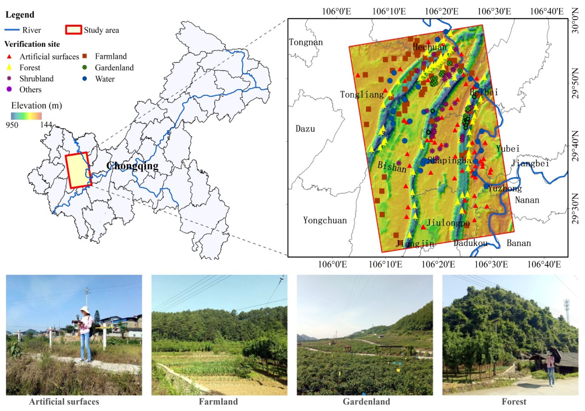
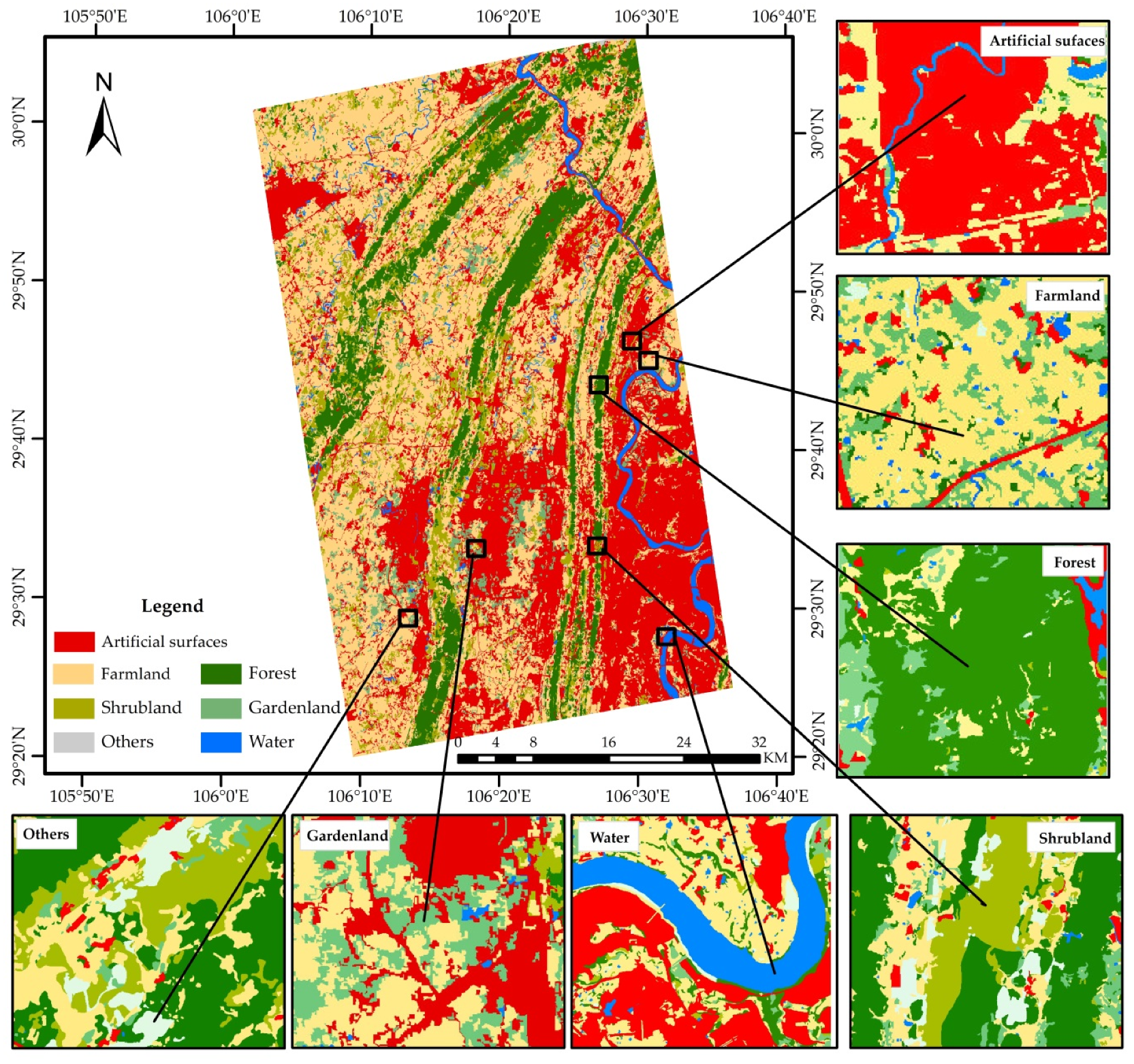
2.1. Study Area
2.2. Data and Processing
3. Methodology
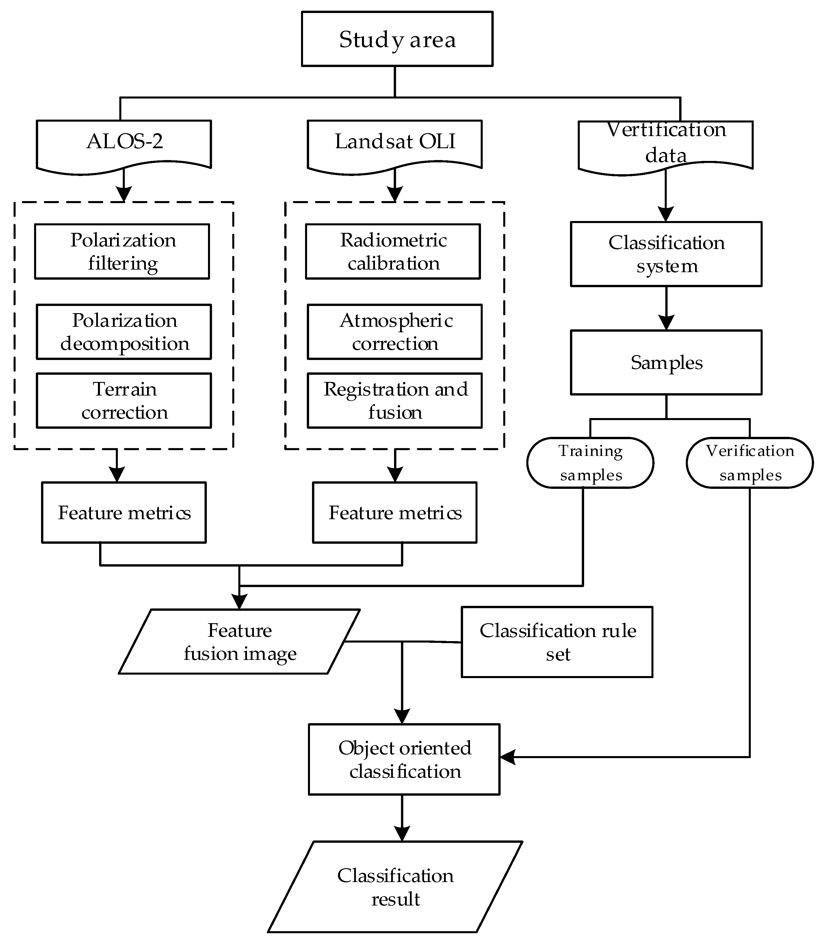
3.1. Proposed Framework
- (1)
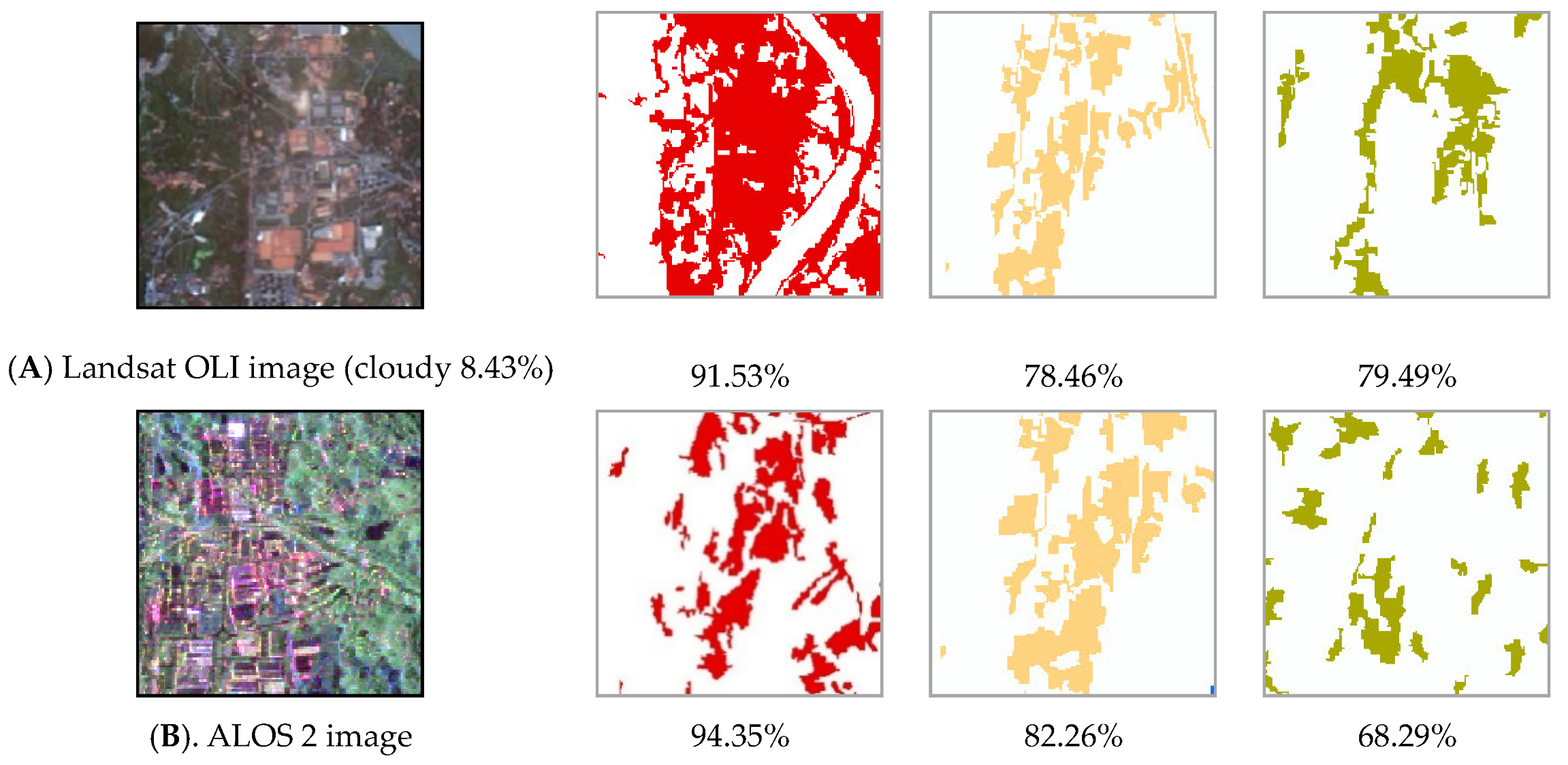
- Landsat 8 OLI feature extraction: to obtain high-quality optical data, the Gram–Schmidt image-fusion method [31,32] was used to fully utilize the spatial texture information via a panchromatic camera and the spectral information from the multispectral camera. On this basis, we calculated spectral features such as brightness value (BG), NDVI; gray-level co-occurrence matrix (GLCM) texture features, contrast, homogeneity, angular second moment, entropy, mean, dissimilarity, variance, and correlation. Simultaneously, we extracted the elevation and slope of different land-cover types in the study area.
- (2)
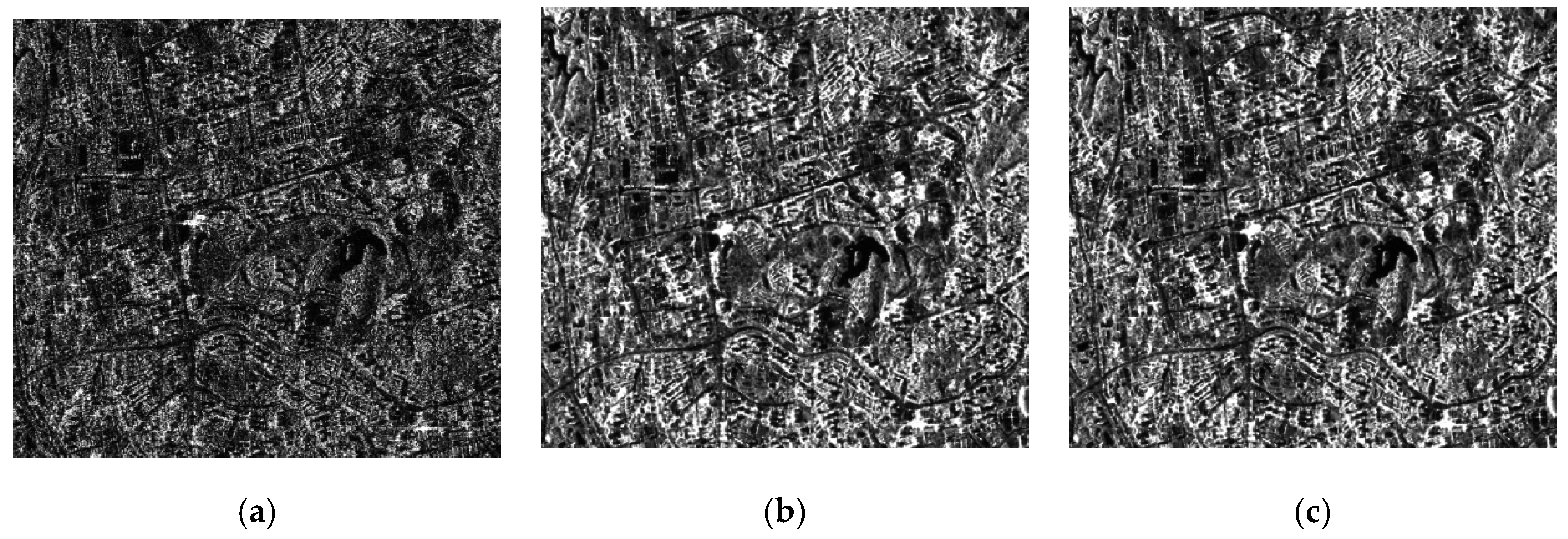
- ALOS 2 SAR data feature extraction: different ground targets in SAR images have different texture features. SAR images contain rich texture information, and texture features are important for image interpretation. We described SAR textures by studying the spatial-correlation properties of grayscale. We calculated the following eight texture features of the ALOS-2 image: contrast, variance, dissimilarity, angular second moment, mean, entropy, homogeneity, and correlation. In addition, the RGB images obtained using the Pauli decomposition were extracted.
- (3)
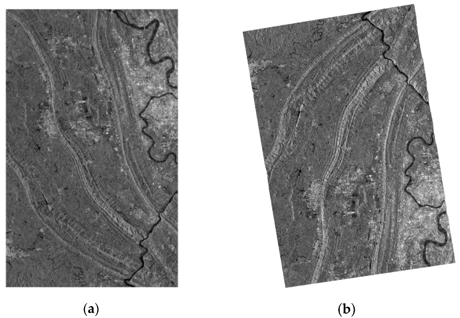
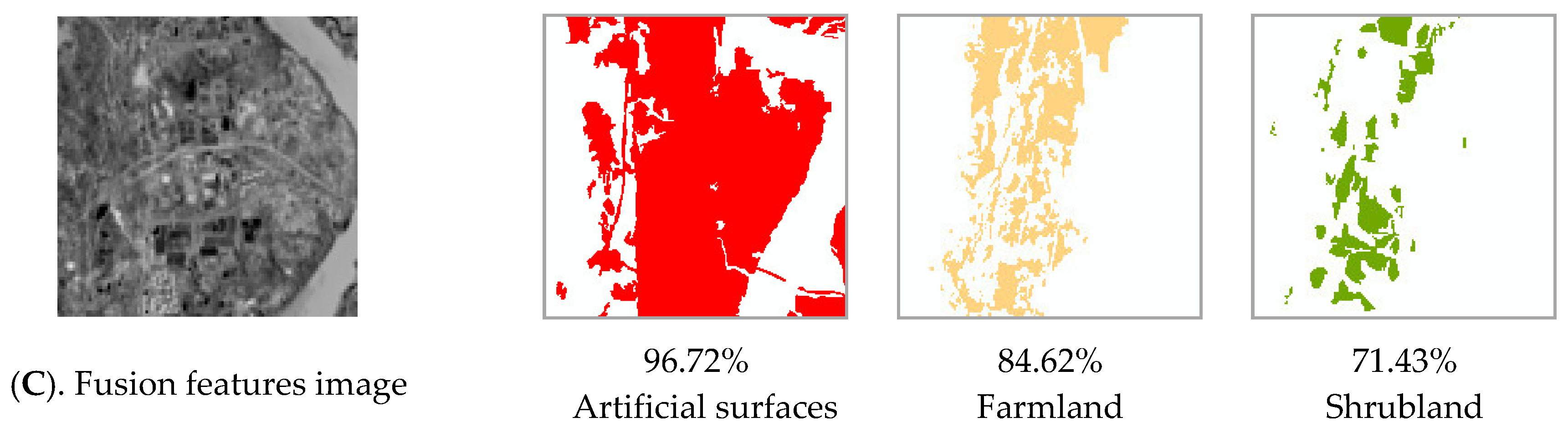
- Optical and SAR image feature level fusion: The OLI multi-spectral images are rich in hue and saturation information compared with high-resolution SAR images, but have less texture information. We can make full use of spectral information of OLI images and high-resolution polarization and texture information of ALOS-2 images, fuse SAR and optical pixels of the same name into multidimensional feature vectors at the feature level. The approach not only improves fusion effect, but also obtains richer feature information. The fusion features are involved in LULC classification to effectively improve accuracy of classification. In this study, two kinds of remote sensing images (ALOS-2 image, OLI image) were preprocessed and the features were extracted respectively. Then the principal component analysis (PCA) of the extracted features was performed, respectively. We retained the first three principal components, in which the features with low correlation and few redundant information. The optical and SAR texture information was superimposed with a certain weight, the spectral information of the first principal component of the optical image was enhanced by a specific weight, and then we added the features of the optical image to the first principal component of the SAR image in order to obtain the enhanced principal component. Then a local energy fusion strategy was used to fuse the texture components of the SAR image and the optical image to obtain the fused texture components. After the processing of spectral and texture components was completed, the contourlet method [33] was adopted to fuse the prepared features. In this paper, we consider the feature information and correlation of images, and get more macroscopic feature level information compared with pixel level fusion.
- (4)
- LULC classification was conducted by using an improved SVM classifier. Owing to the nonlinear nature of high-resolution remote-sensing data, the classification of remote-sensing data is mostly a nonlinear classification problem. To solve the classification of linear indivisible problems, we can improve the parameters of the radial basis function (RBF) in the SVM classifier.
- (5)
- Analysis and comparison of the results. We compared and analyzed the results derived using the method proposed in this study, where the classification results was obtained using a single image.
3.2. Classification System
3.3. Improved SVM Model
4. Results
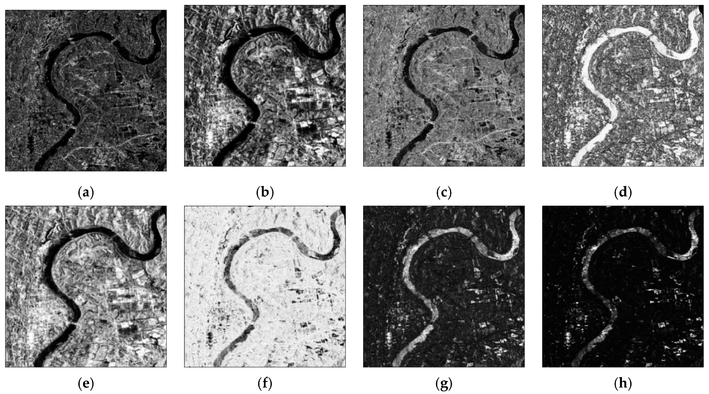
4.1. Features Metrics and Extraction
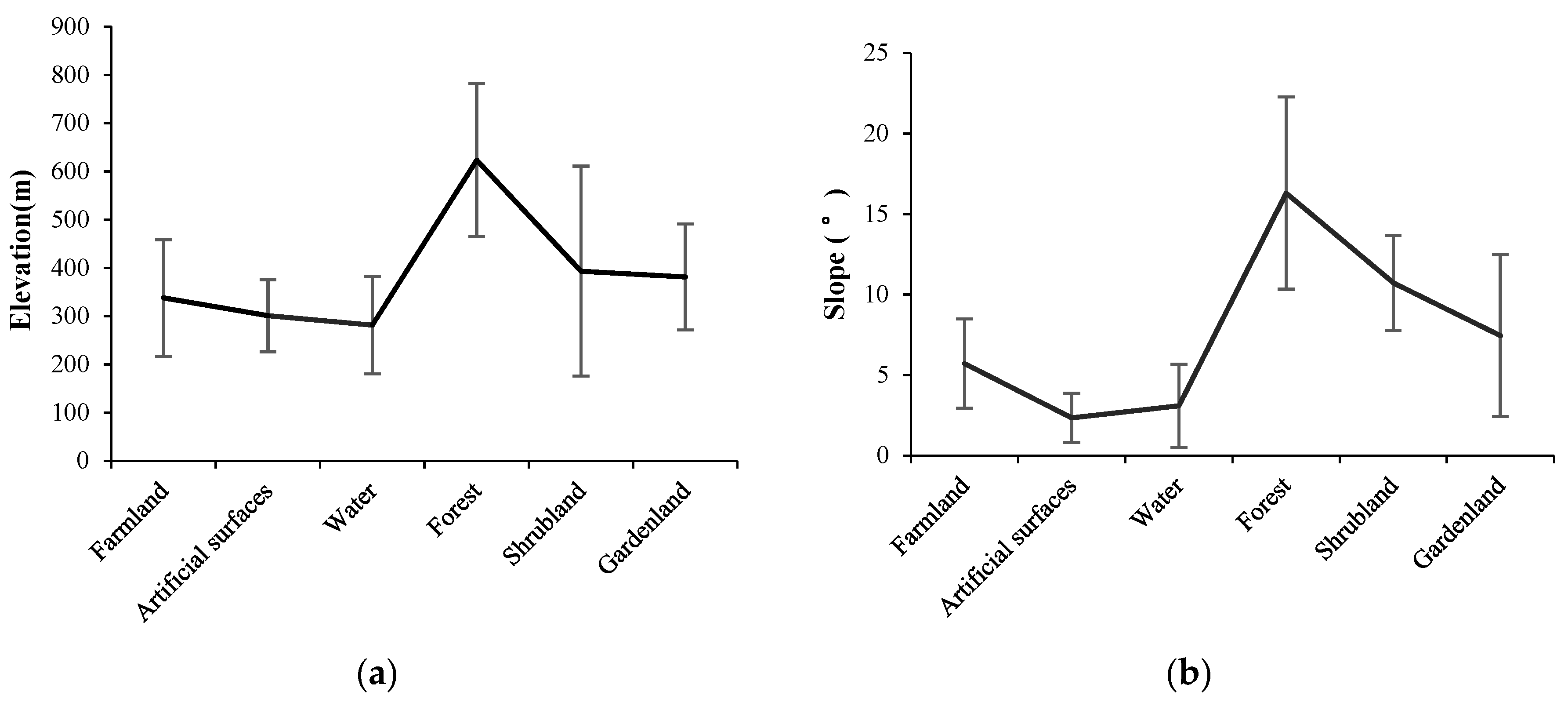
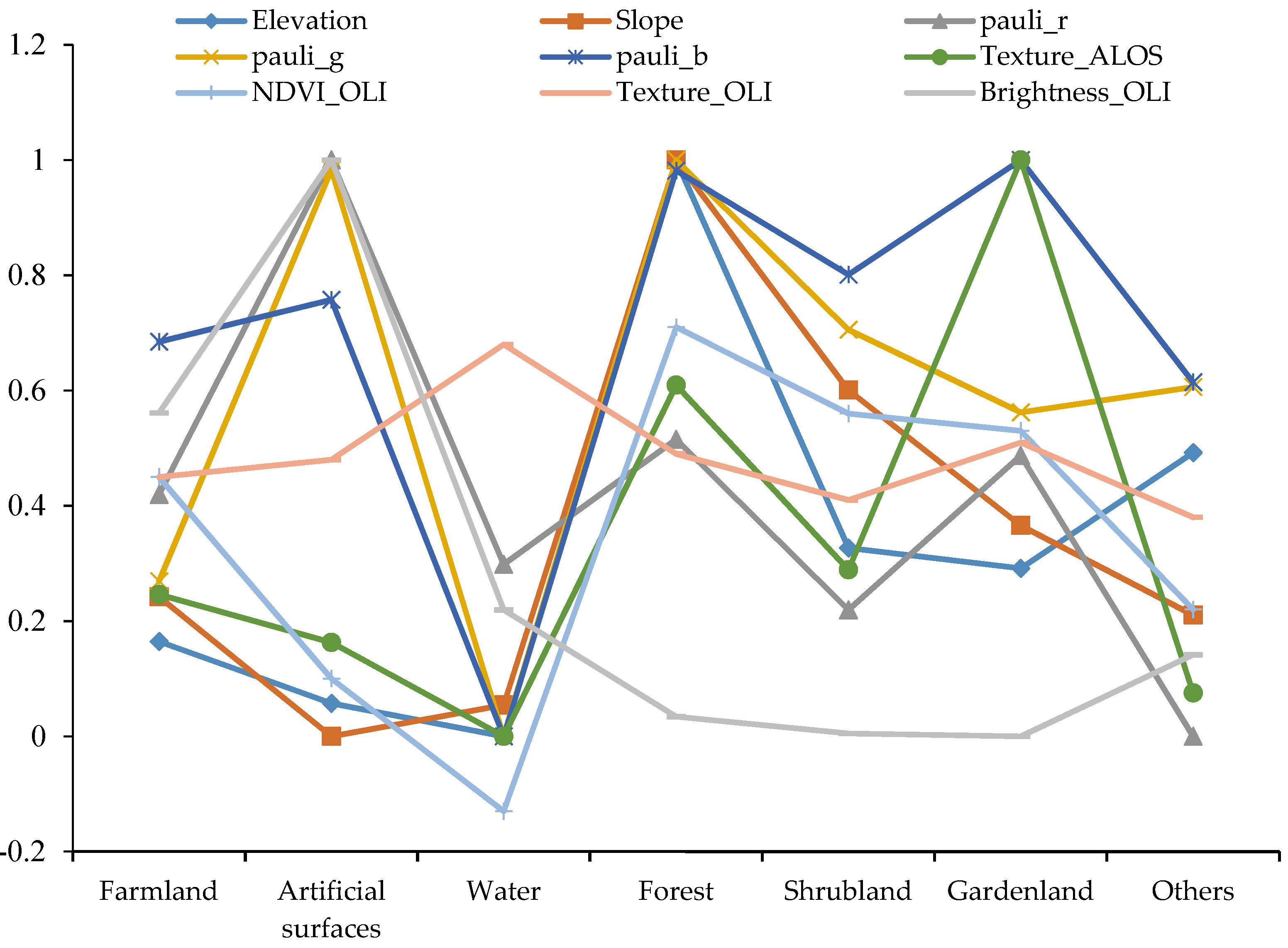
4.1.1. Geoscience Auxiliary Features
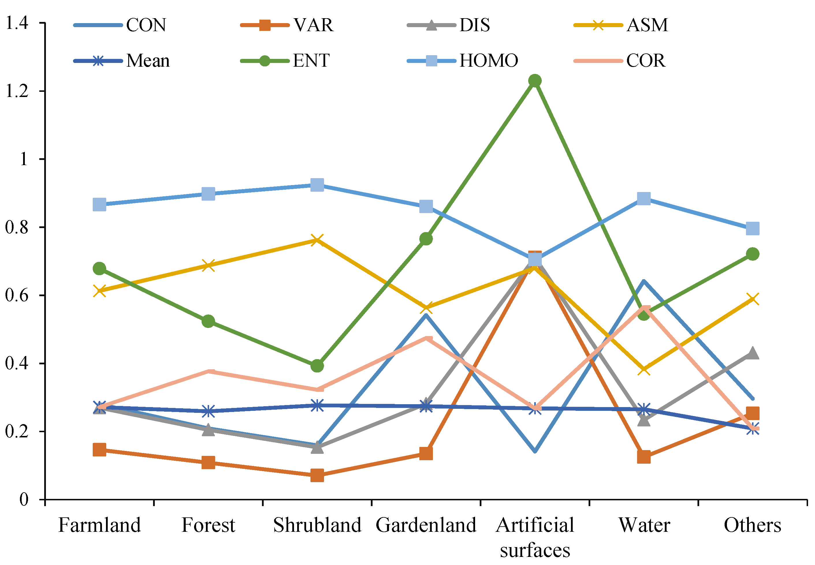
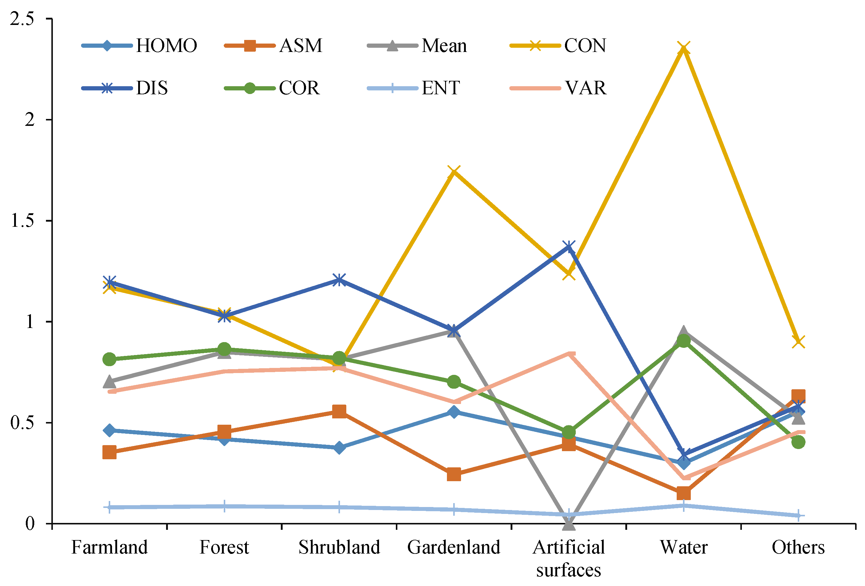
4.1.2. Texture Features of SAR and Optical Images
4.1.3. Feature Analysis
4.2. Classification Results and Accuracy of the Proposed Method
4.3. Accuracy Assessment
5. Discussion
5.1. Classification Method and Effect Evaluation
5.2. Advantages and Disadvantages of the SVM Model
5.3. Limitations
6. Conclusions
Author Contributions
Funding
Conflicts of Interest
References
- He, G.; Feng, X.; Xiao, P.; Xia, Z.; Wang, Z.; Chen, H.; Li, H.; Guo, J. Dry and wet snow cover mapping in mountain areas using SAR and optical remote sensing data. IEEE J. Sel. Top. Appl. Earth Obs. Remote Sens. 2017, 10, 2575–2588. [Google Scholar] [CrossRef]
- Araya-López, R.A.; Lopatin, J.; Fassnacht, F.E.; Hernández, H.J. Monitoring Andean high altitude wetlands in central Chile with seasonal optical data: A comparison between Worldview-2 and Sentinel-2 imagery. ISPRS J. Photogramm. Remote Sens. 2018, 145, 213–224. [Google Scholar] [CrossRef]
- Luo, K.; Li, B.; Moiwo, J. Monitoring Land-Use/Land-Cover changes at a provincial large scale using an object-oriented technique and medium-resolution remote-sensing images. Remote Sens. 2018, 10, 2012. [Google Scholar] [CrossRef] [Green Version]
- Stewart, J.C.; Zhou, W.; Santi, P.M. Using an integrated remote sensing approach for identification of bedrock and alluvium along the Front Range mountains, Colorado. J. Appl. Remote Sens. 2017, 11, 1. [Google Scholar] [CrossRef]
- Gopal, S.; Woodcock, C.E.; Strahler, A.H. Fuzzy neural net-work classification of global land cover from a 1° AVHRR data set. Remote Sens. Environ. 1999, 67, 230–243. [Google Scholar] [CrossRef]
- Gilbertson, J.K.; Kemp, J.; van Niekerk, A. Effect of pan-sharpening multi-temporal Landsat 8 imagery for crop type differentiation using different classification techniques. Comput. Electron. Agric. 2017, 134, 151–159. [Google Scholar] [CrossRef] [Green Version]
- Wang, T.T.; Li, S.S.; Li, A.; Feng, X.X.; Wu, Y.W. Land cover classification in Beijing using Landsat 8 image. J. Image Graph. 2015, 20, 1275–1284. [Google Scholar]
- Liu, H.; Wang, F.; Yang, S.; Hou, B.; Jiao, L.; Yang, R. Fast semisupervised classification using histogram-based density estimation for large-scale polarimetric SAR data. IEEE Geosci. Remote Sens. Lett. 2019, 16, 1844–1848. [Google Scholar] [CrossRef]
- Sica, F.; Pulella, A.; Nannini, M.; Pinheiro, M.; Rizzoli, P. Repeat-pass SAR interferometry for land cover classification: A methodology using Sentinel-1 Short-Time-Series. Remote Sens. Environ. 2019, 232, 111277. [Google Scholar] [CrossRef]
- Hoang, H.K.; Bernier, M.; Duchesne, S.; Tran, Y.M. Rice mapping using RADARSAT-2 dual- and quad-pol data in a complex land-use watershed: Cau River Basin (Vietnam). IEEE J. Sel. Top. Appl. Earth Obs. Remote Sens. 2016, 9, 3082–3096. [Google Scholar] [CrossRef] [Green Version]
- Tavares, P.A.; Beltrão, N.E.S.; Guimarães, U.S.; Teodoro, A.C. Integration of Sentinel-1 and Sentinel-2 for classification and LULC mapping in the urban area of Belém, Eastern Brazilian Amazon. Sensors 2019, 19, 1140. [Google Scholar] [CrossRef] [Green Version]
- Yin, J.; Yang, J.; Zhang, Q. Assessment of GF-3 polarimetric SAR data for physical scattering mechanism analysis and terrain classification. Sensors 2017, 17, 2785. [Google Scholar] [CrossRef] [Green Version]
- Li, D.; Zhang, Y. Adaptive model-based classification of PolSAR data. IEEE Trans. Geosci. Remote Sens. 2018, 56, 6940–6955. [Google Scholar] [CrossRef]
- Chatziantoniou, A.; Psomiadis, E.; Petropoulos, G.P. Co-orbital Sentinel 1 and 2 for LULC mapping with emphasis on wetlands in a Mediterranean setting based on machine learning. Remote Sens. 2017, 9, 1259. [Google Scholar] [CrossRef] [Green Version]
- Hagensieker, R.; Roscher, R.; Rosentreter, J.; Jakimow, B.; Waske, B. Tropical land use land cover mapping in Pará (Brazil) using discriminative Markov random fields and multi-temporal TerraSAR-X data. Int. J. Appl. Earth Obs. Geoinf. 2017, 63, 244–256. [Google Scholar] [CrossRef] [Green Version]
- Hütt, C.; Koppe, W.; Miao, Y.; Bareth, G. Best accuracy Land Use/Land Cover (LULC) classification to derive crop types using multitemporal, multisensor, and multi-polarization SAR satellite images. Remote Sens. 2016, 8, 684. [Google Scholar] [CrossRef] [Green Version]
- Sameen, M.; Nahhas, F.H.; Buraihi, F.H.; Pradhan, B.; Shariff, A.R.B.M. A refined classification approach by integrating Landsat Operational Land Imager (OLI) and RADARSAT-2 imagery for land-use and land-cover mapping in a tropical area. Int. J. Remote Sens. 2016, 37, 2358–2375. [Google Scholar] [CrossRef]
- Sanli, F.B.; Esetlili, T.; Sunar, F.; Abdikan, S. Evaluation of image fusion methods using PALSAR, RADARSAT-1 and SPOT images for land use/land cover classification. J. Indian Soc. Remote Sens. 2016, 45, 591–601. [Google Scholar] [CrossRef]
- Ghassemian, H. A review of remote sensing image fusion methods. Inf. Fusion 2016, 32, 75–89. [Google Scholar] [CrossRef]
- Zhang, R.; Zhou, Y.; Luo, H.; Wang, F.; Wang, S. Estimation and analysis of spatiotemporal dynamics of the net primary productivity integrating efficiency model with process model in Karst Area. Remote Sens. 2017, 9, 477. [Google Scholar] [CrossRef] [Green Version]
- Xiao, Q.; Tao, J.; Xiao, Y.; Qian, F. Monitoring vegetation cover in Chongqing between 2001 and 2010 using remote sensing data. Environ. Monit. Assess. 2017, 189, 189. [Google Scholar] [CrossRef] [PubMed]
- Anderson, G.P.; Felde, G.W.; Hoke, M.L.; Ratkowski, A.J.; Cooley, T.W.; Chetwynd, J.J.H.; Gardner, J.A.; Adler-Golden, S.M.; Matthew, M.W.; Berk, A.; et al. MODTRAN4-based atmospheric correction algorithm: FLAASH (fast line-of-sight atmospheric analysis of spectral hypercubes). Proc. SPIE Int. Soc. Opt. Eng. 2002, 4725, 65–71. [Google Scholar]
- Koyama, C.N.; Watanabe, M.; Hayashi, M.; Ogawa, T.; Shimada, M. Mapping the spatial-temporal variability of tropical forests by ALOS-2 L-band SAR big data analysis. Remote Sens. Environ. 2019, 233, 111372. [Google Scholar] [CrossRef]
- Cloude, S.; Pottier, E. A review of target decomposition theorems in radar polarimetry. IEEE Trans. Geosci. Remote Sens. 1996, 34, 498–518. [Google Scholar] [CrossRef]
- Freeman, A.; Durden, S.L. Three-component scattering model to describe polarimetric SAR data. In Proceedings of the International Society for Optical Engineering, San Diego, CA, USA, 12 February 1993; Volume 1748, pp. 213–224. [Google Scholar]
- Yamaguchi, Y.; Moriyama, T.; Ishido, M.; Yamada, H. Four-component scattering model for polarimetric SAR image decomposition. IEEE Trans. Geosci. Remote Sens. 2005, 43, 1699–1706. [Google Scholar] [CrossRef]
- Cloude, S.; Pottier, E. An entropy based classification scheme for land applications of polarimetric SAR. IEEE Trans. Geosci. Remote Sens. 1997, 35, 68–78. [Google Scholar] [CrossRef]
- Cloude, S.R. Radar target decomposition theorems. Inst. Electr. Eng. Electron. Lett. 1985, 21, 22–24. [Google Scholar]
- Lee, J.S.; Pottier, E. Polarimetric Radar Imaging: From Basics to Applications; CRC Press, Taylor & Francis Group: Boca Raton, FL, USA, 2009. [Google Scholar]
- Ghasemi, N.; Mohammadzadeh, A.; Sahebi, M.R. Assessment of different topographic correction methods in ALOS AVNIR-2 data over a forest area. Int. J. Digit. Earth 2013, 6, 504–520. [Google Scholar] [CrossRef]
- Yilmaz, V.; Yilmaz, C.S.; Güngör, O.; Shan, J. A genetic algorithm solution to the gram-schmidt image fusion. Int. J. Remote Sens. 2019, 41, 1458–1485. [Google Scholar] [CrossRef]
- Guo, B.; Wen, Y. An optimal monitoring model of desertification in naiman banner based on feature space utilizing landsat8 oli image. IEEE Access 2020, 8, 4761–4768. [Google Scholar] [CrossRef]
- Chu, T.; Tan, Y.; Liu, Q.; Bai, B. Novel fusion method for SAR and optical images based on non-subsampled shearlet transform. Int. J. Remote Sens. 2020, 41, 4590–4604. [Google Scholar] [CrossRef]
- Jun, C.; Ban, Y.; Li, S. Open access to Earth land-cover map. Nature 2014, 514, 434. [Google Scholar] [CrossRef] [PubMed] [Green Version]
- Cortes, C.; Vapnik, V. Support-vector networks. Mach. Learn 1995, 20, 273–297. [Google Scholar] [CrossRef]
- Devroye, L.; Györfi, L.; Lugosi, G. Vapnik-Chervonenkis theory. In A Probabilistic Theory of Pattern Recognition; Springer: New York, NY, USA, 1996; pp. 187–213. [Google Scholar]
- Kalantar, B.; Pradhan, B.; Naghibi, S.A.; Motevalli, A.; Mansor, S. Assessment of the effects of training data selection on the landslide susceptibility mapping: A comparison between support vector machine (SVM), logistic regression (LR) and artificial neural networks (ANN). Geomat. Nat. Hazards Risk 2017, 9, 49–69. [Google Scholar] [CrossRef]
- Zhang, R.; Ma, J. Feature selection for hyperspectral data based on recursive support vector machines. Int. J. Remote Sens. 2009, 30, 3669–3677. [Google Scholar] [CrossRef]
- Liang, Y.; Lee, H.; Lim, S.; Lin, W.; Lee, K.; Wu, C. Proper orthogonal decomposition and its applications—Part I: Theory. J. Sound Vib. 2002, 252, 527–544. [Google Scholar] [CrossRef]
- Zhao, G.; Maclean, A.L. A comparison of canonical discriminant analysis and principal component analysis for spectral transformation. Photogramm. Eng. Remote Sens. 2000, 66, 841–847. [Google Scholar]
- Metternicht, G.; Zinck, J. Remote sensing of soil salinity: Potentials and constraints. Remote Sens. Environ. 2003, 85, 1–20. [Google Scholar] [CrossRef]


| Advanced Land Observing Satellite 2 (ALOS-2) SAR Data | |||||
| Acquisition Date | Mode | Orbit | Incidence angle | Pixel Spacing (m) | Polarization |
| 2015-03-27 | Ultra-Fine | Descending | 8°–70° | 2.861 × 3.112 | HH/VH/VV/HV |
| Landsat 8 Operational Land Imager (OLI) Data | |||||
| Acquisition Date | Path | Row | Resolution (m) | Bands | Cloud Cover (%) |
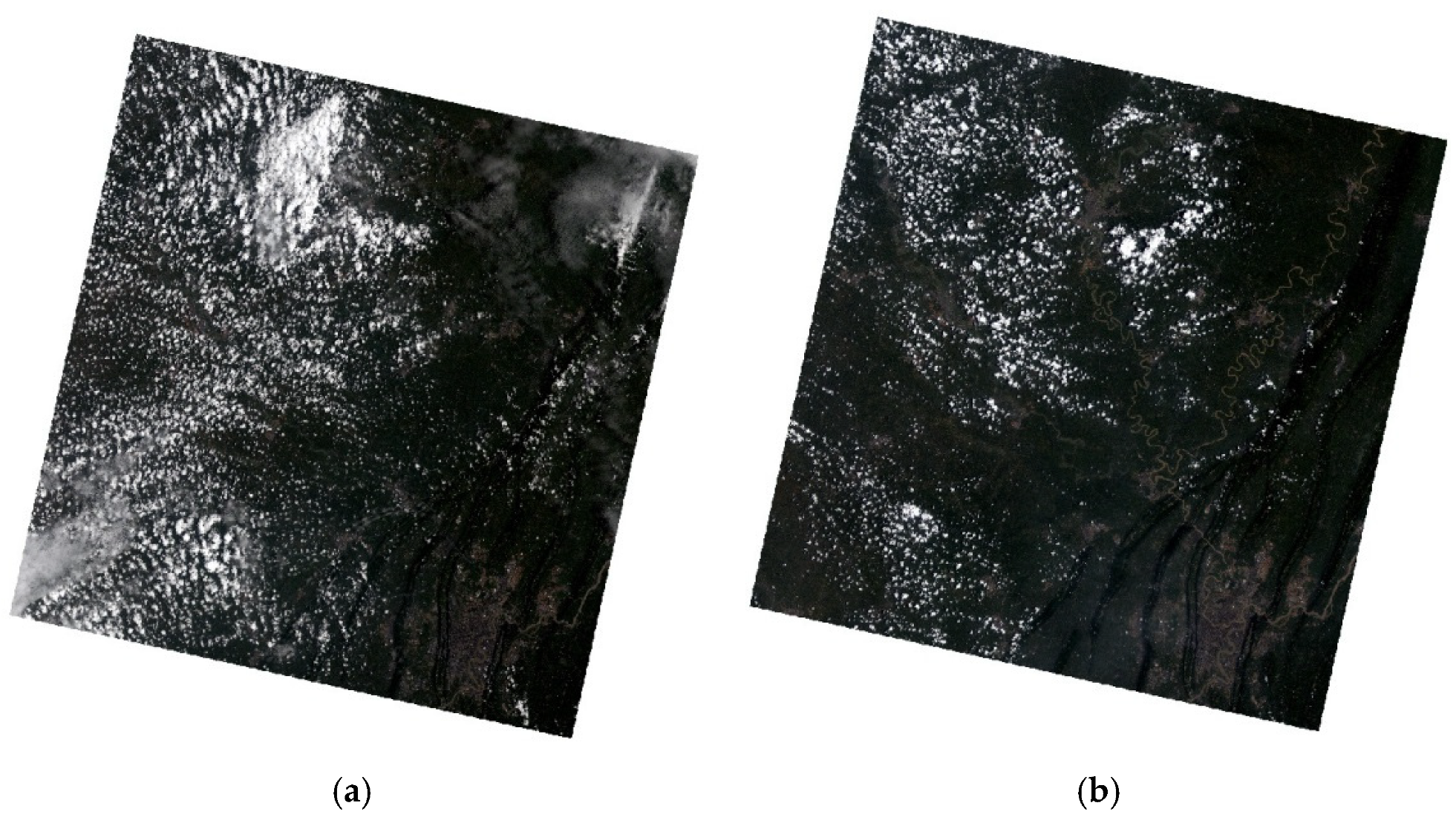
| 2015-06-22 | 126 | 40 | 30 × 30 | 1–5, 7 | 8.43% |
| 2015-07-08 | 126 | 40 | 30 × 30 | 1–5, 7 | 26.28% |
| Land Cover Types | Type Description |
|---|---|
| Farmland | Land where crops are grown, including cultivated land, newly reclaimed land, recreational land. |
| Gardenland | Planting perennial woody and herbaceous crops mainly for collecting fruits, leaves and rhizomes with a coverage greater than 50%. |
| Forest | Growing trees, bamboos, etc., tree height is greater than 5 m. |
| Shrubland | Woods less than 5 m tall, short and tufted woody and herbaceous plants. |
| Artificial Surfaces | Land to build buildings and structures. |
| Water | Land for rivers, reservoirs, pits, water conservancy facilities and floodplains. |
| Others | Unused or hard-to-use land, including marshes, saline land. |
| Forest | Shrubland | Gardenland | Farmland | Water | Artificial Surface | Others | Total | UA (%) | |
|---|---|---|---|---|---|---|---|---|---|
| Forest | 49 | 7 | 1 | 2 | 0 | 1 | 0 | 59 | 83.05 |
| Shrubland | 4 | 30 | 3 | 2 | 0 | 0 | 0 | 39 | 76.92 |
| Gardenland | 0 | 1 | 19 | 3 | 0 | 0 | 0 | 23 | 82.61 |
| Farmland | 0 | 4 | 5 | 55 | 1 | 0 | 0 | 65 | 84.62 |
| Water | 0 | 0 | 0 | 0 | 27 | 1 | 0 | 28 | 96.43 |
| Artificial surface | 0 | 0 | 0 | 2 | 0 | 59 | 0 | 61 | 96.72 |
| Others | 0 | 0 | 0 | 1 | 0 | 0 | 8 | 9 | 88.89 |
| Total | 53 | 42 | 28 | 65 | 28 | 61 | 8 | 284 | |
| PA(%) | 92.45 | 71.43 | 67.86 | 84.62 | 96.43 | 96.72 | 100.00 | ||
| OA: 86.97% | Kappa coefficient: 0.8447 | ||||||||
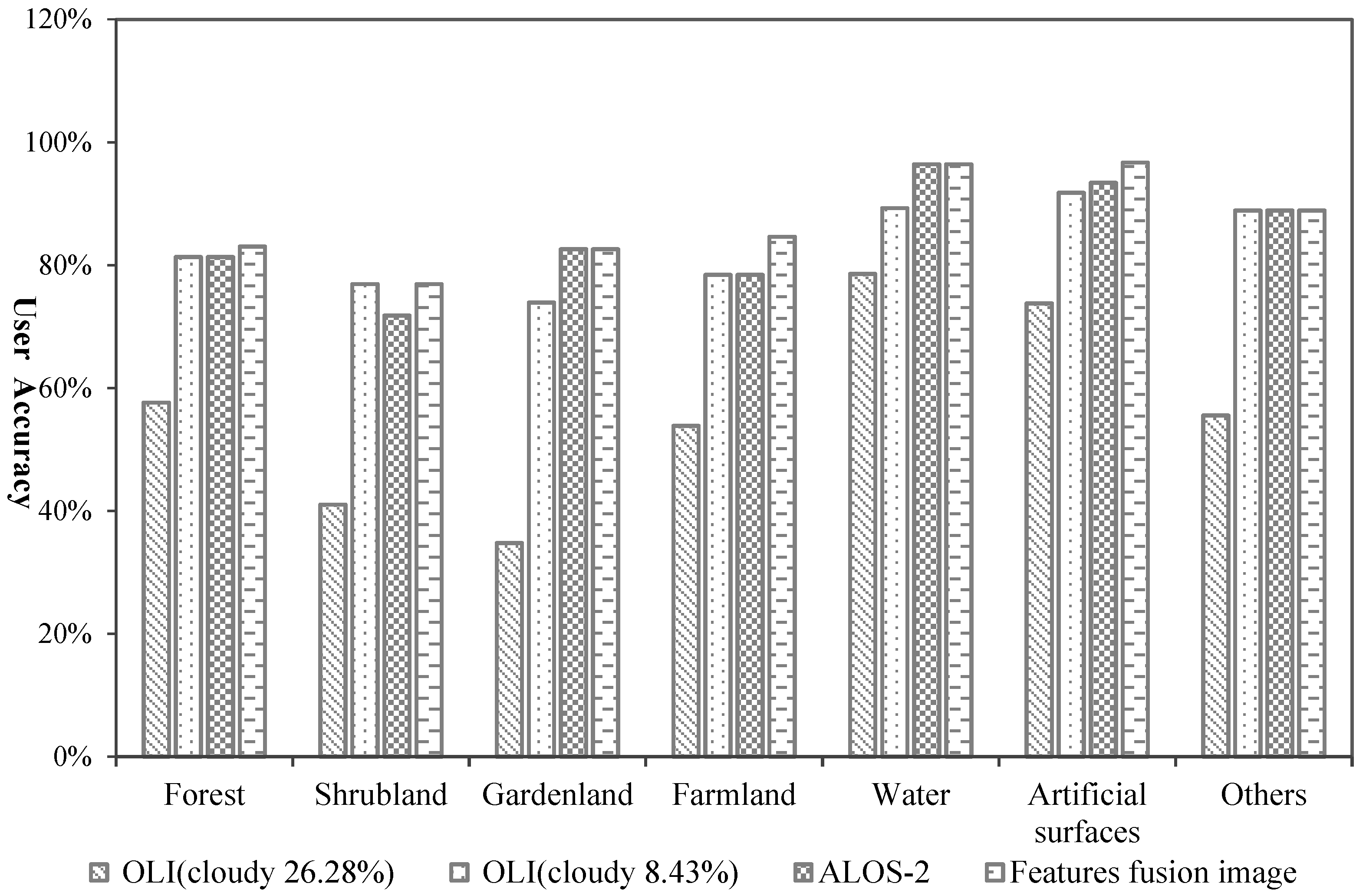
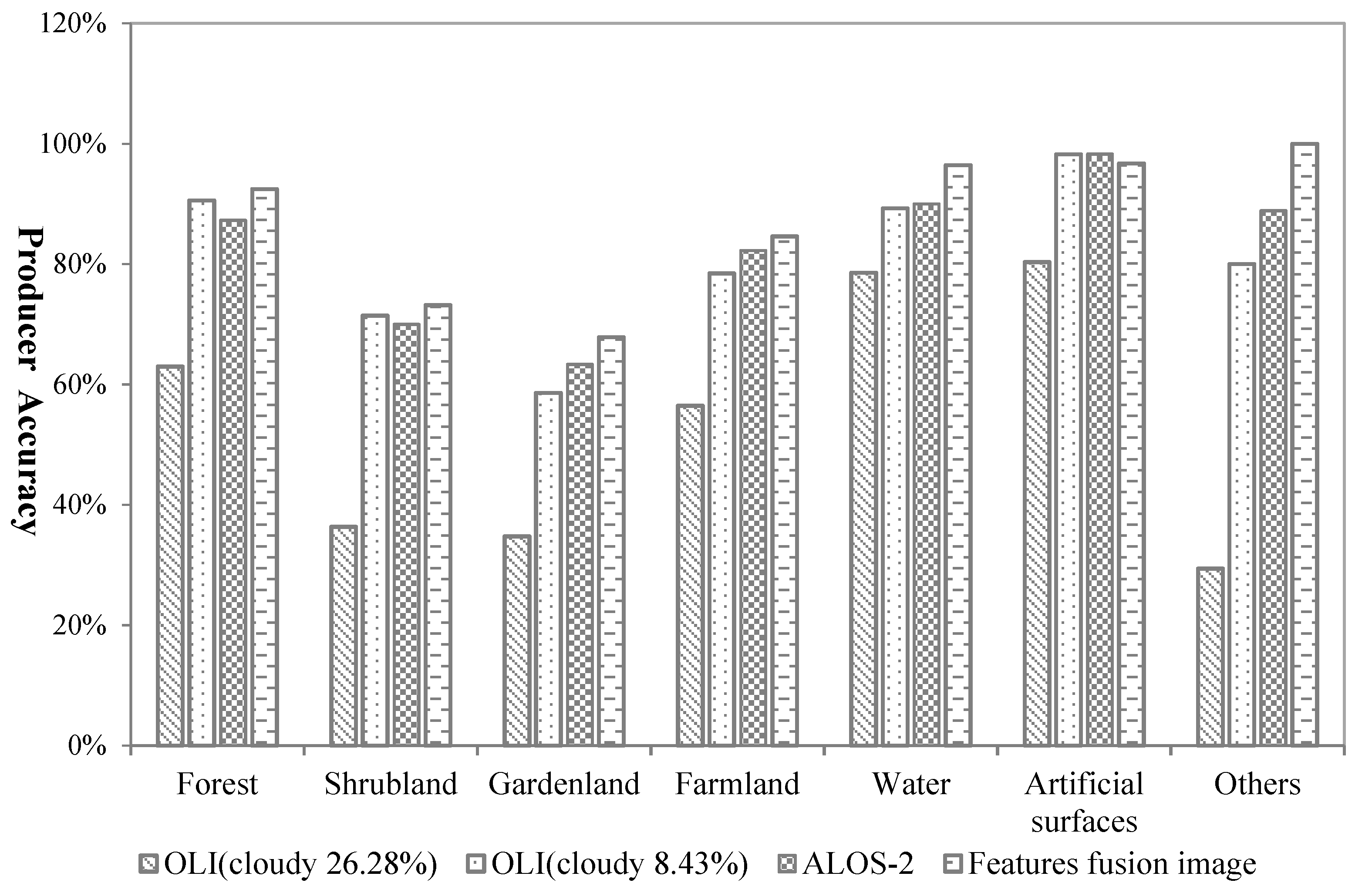
| Experimental Data | Evaluation Index | Forest | Shrubland | Gardenland | Farmland | Water | Artificial Surfaces | Others |
|---|---|---|---|---|---|---|---|---|
| Landsat OLI (cloudiness: 26.28%) | UA (%) | 64.41 | 51.28 | 47.83 | 64.62 | 78.57 | 80.33 | 55.56 |
| PA (%) | 76.00 | 43.48 | 44.00 | 65.63 | 81.48 | 84.48 | 41.67 | |
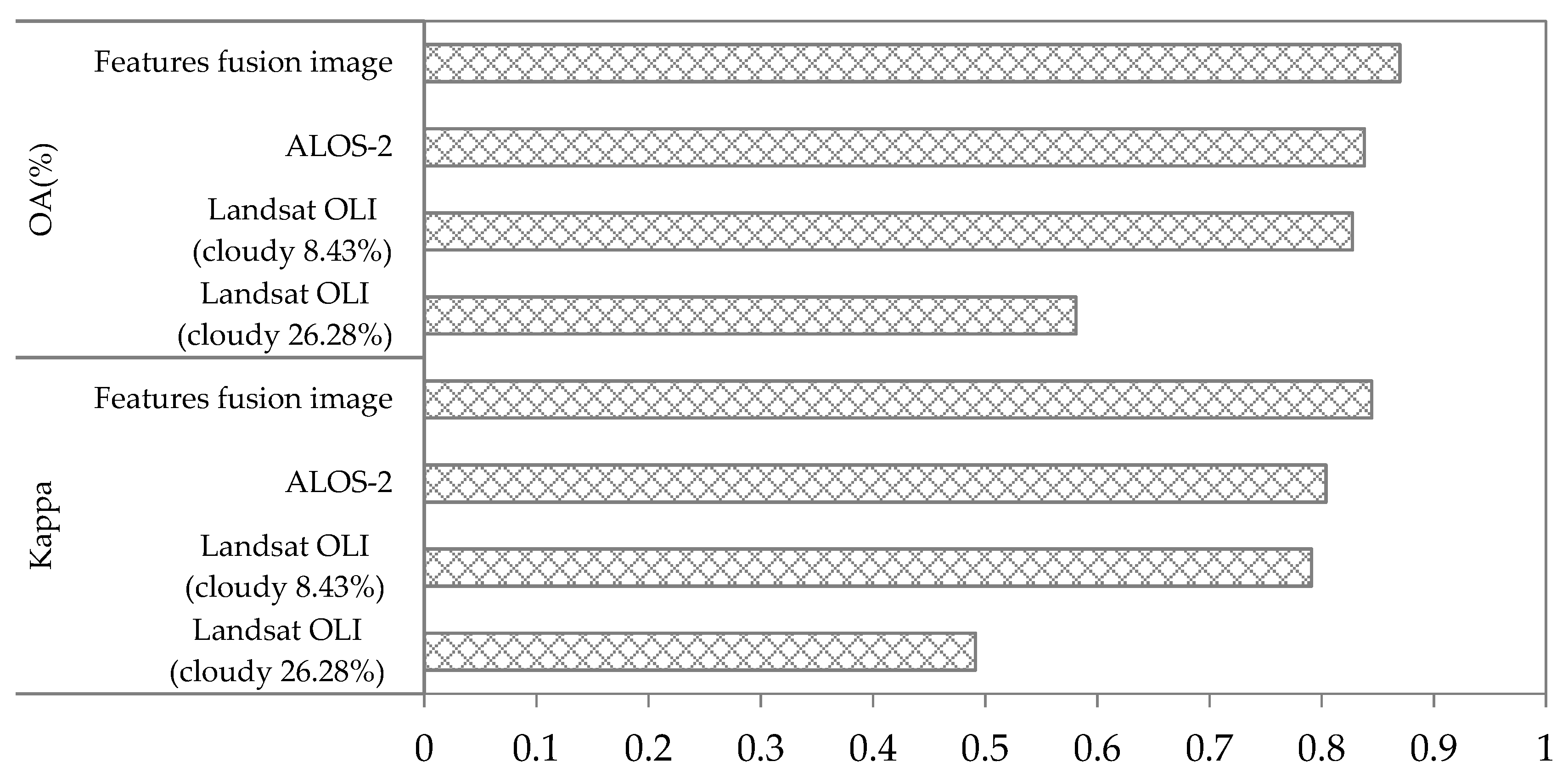
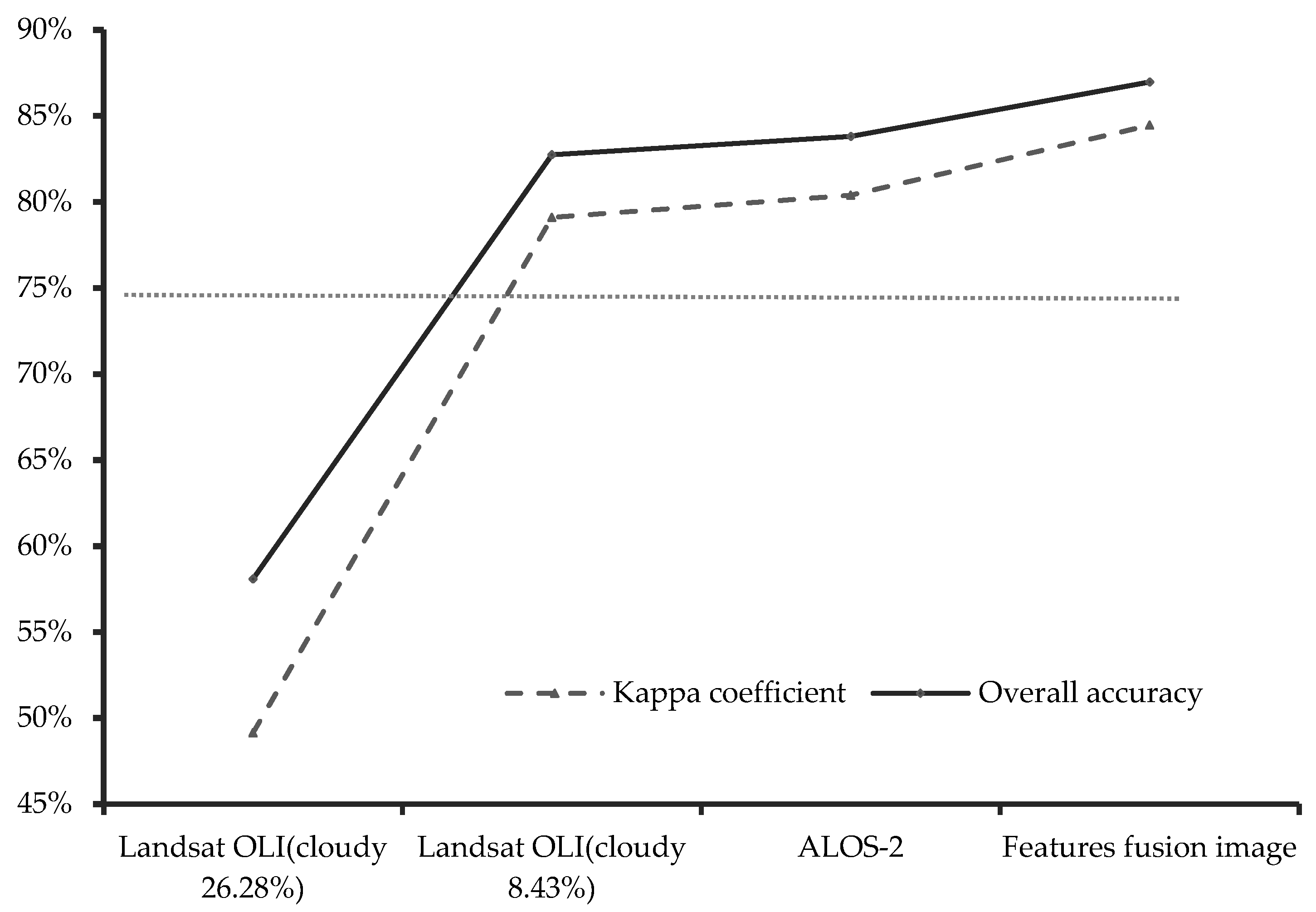
| OA | 0.491 | |||||||
| Kappa | 0.585 | |||||||
| Landsat OLI (cloudiness: 8.43%) | UA (%) | 81.36 | 79.49 | 73.91 | 78.46 | 89.29 | 91.80 | 88.89 |
| PA (%) | 90.57 | 70.45 | 56.67 | 78.46 | 89.29 | 91.53 | 80.00 | |
| OA | 0.827 | |||||||
| Kappa | 0.796 | |||||||
| ALOS-2 | UA (%) | 81.36 | 71.79 | 82.61 | 78.46 | 96.43 | 93.44 | 88.89 |
| PA (%) | 87.27 | 68.29 | 63.33 | 82.26 | 90.00 | 94.35 | 88.89 | |
| OA | 0.838 | |||||||
| Kappa | 0.840 | |||||||
| Features fusion image | UA (%) | 83.05 | 76.92 | 82.61 | 84.62 | 96.43 | 96.72 | 88.89 |
| PA (%) | 92.45 | 71.43 | 67.86 | 84.62 | 96.43 | 96.72 | 100.00 | |
| OA | 0.870 | |||||||
| Kappa | 0.845 | |||||||
© 2020 by the authors. Licensee MDPI, Basel, Switzerland. This article is an open access article distributed under the terms and conditions of the Creative Commons Attribution (CC BY) license (http://creativecommons.org/licenses/by/4.0/).
Share and Cite
Zhang, R.; Tang, X.; You, S.; Duan, K.; Xiang, H.; Luo, H. A Novel Feature-Level Fusion Framework Using Optical and SAR Remote Sensing Images for Land Use/Land Cover (LULC) Classification in Cloudy Mountainous Area. Appl. Sci. 2020, 10, 2928. https://doi.org/10.3390/app10082928
Zhang R, Tang X, You S, Duan K, Xiang H, Luo H. A Novel Feature-Level Fusion Framework Using Optical and SAR Remote Sensing Images for Land Use/Land Cover (LULC) Classification in Cloudy Mountainous Area. Applied Sciences. 2020; 10(8):2928. https://doi.org/10.3390/app10082928
Chicago/Turabian StyleZhang, Rui, Xinming Tang, Shucheng You, Kaifeng Duan, Haiyan Xiang, and Hongxia Luo. 2020. "A Novel Feature-Level Fusion Framework Using Optical and SAR Remote Sensing Images for Land Use/Land Cover (LULC) Classification in Cloudy Mountainous Area" Applied Sciences 10, no. 8: 2928. https://doi.org/10.3390/app10082928