A Boundary Distance-Based Symbolic Aggregate Approximation Method for Time Series Data


1
School of Computer Science, China University of Geosciences (Wuhan), 388 Lumo Road, Wuhan 430074, China
2
Department of Computer Science, University of Idaho, 875 Perimeter Drive MS 1010, Moscow, ID 83844-1010, USA
*
Author to whom correspondence should be addressed.
Algorithms 2020, 13(11), 284; https://doi.org/10.3390/a13110284
Submission received: 11 September 2020
/
Revised: 25 October 2020
/
Accepted: 26 October 2020
/
Published: 9 November 2020
(This article belongs to the Special Issue Algorithms and Applications of Time Series Analysis)
Abstract
:A large amount of time series data is being generated every day in a wide range of sensor application domains. The symbolic aggregate approximation (SAX) is a well-known time series representation method, which has a lower bound to Euclidean distance and may discretize continuous time series. SAX has been widely used for applications in various domains, such as mobile data management, financial investment, and shape discovery. However, the SAX representation has a limitation: Symbols are mapped from the average values of segments, but SAX does not consider the boundary distance in the segments. Different segments with similar average values may be mapped to the same symbols, and the SAX distance between them is 0. In this paper, we propose a novel representation named SAX-BD (boundary distance) by integrating the SAX distance with a weighted boundary distance. The experimental results show that SAX-BD significantly outperforms the SAX representation, ESAX representation, and SAX-TD representation.
1. Introduction
Time series data are being generated every day in a wide range of application domains [1], such as bioinformatics, finance, engineering, etc. [2]. The parallel explosions of interest in streaming data and data mining of time series [3,4,5,6,7,8,9] have had little intersection. Time series classification methods can be divided into three main categories [10]: feature based, model based and distance based. There are many methods for feature extraction, for example: (1) spectral analysis such as discrete Fourier transform (DFT) [11], (2) discrete wavelet transform (DWT) [12], where features of the frequency domain are considered, and (3) singular value decomposition (SVD) [13], where eigenvalue analysis is carried out in order to find an optimal set of features. The model-based classification methods include auto-regressive models [14,15] or hidden Markov models [16], among others. In distance-based methods, 1-NN [1] has been a widely used method due to its simplicity and good performance.
Until now, almost all the research in distance-based classification has been oriented to defining different types of distance measures and then exploiting them within the 1-NN classifiers. The 1-NN classifier is probably the simplest classifier among all classifiers, while its performance is also good. Dynamic Time Warping(DTW) [17] as a distance method used for 1-NN classifier makes the classification accuracy reach the maximum at that time. However, due to the high dimensions, high volume, high feature correlation, and multiple noises, it has brought great challenges to the classification of time series, and even makes the DTW unusable. In fact, all non-trivial data mining and indexing algorithms decrease exponentially with dimensions. For example, above 16–20 dimensions, the index structure will be degraded to sequential scanning [18]. In order to reduce the time series dimensions and have a low bound to the Euclidean distance. The Piecewise Aggregate Approximation(PAA) [19] and Symbolic Aggregate Approximate(SAX) [20] were brought up. The distance in the SAX representation has a lower bound to the Euclidean distance. Therefore, the SAX representation speeds up the data mining process of time series data while maintaining the quality of the data mining results. SAX has been widely used in mobile data management [21], financial investment [22], feature extraction [23]. In recent years, with the popularity of deep learning, applying deep learning methods to multivariate time series classification has also received attention [24].
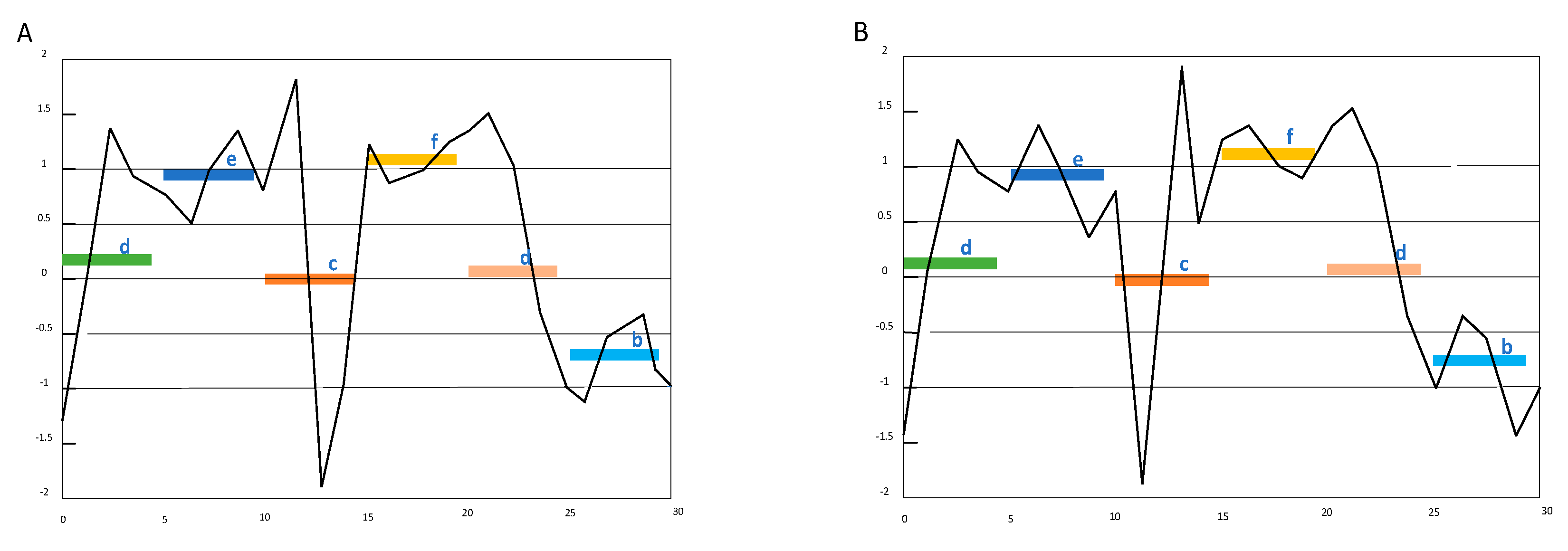
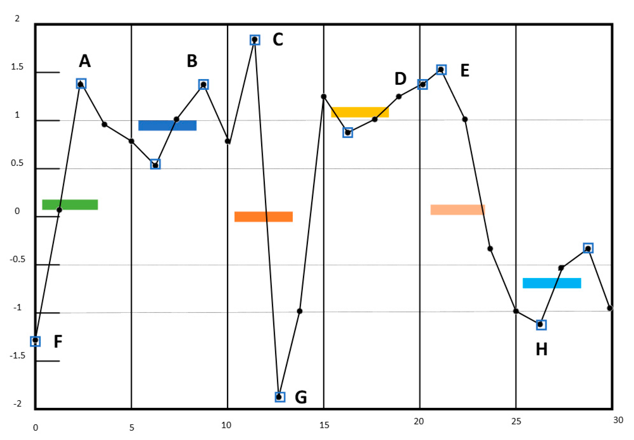
SAX allows a time series of arbitrary length n to be reduced to a string of arbitrary length w [20] (w < n, typically w << n). The alphabet size α is also an arbitrary integer. The SAX representation has a major limitation. In the SAX representation, symbols are mapped from the average values of segments, and some important features may loss. For example, in Figure 1, if w = 6 and α = 6, time series a represented as ‘decfdb’.
However, it can be clearly seen from the Figure 1 that the time series changes drastically. Therefore, a compromise is needed to reduce the dimension of time series while improving the accuracy. ESAX representation can express the characteristics of time series in more detail [25]. It chooses a maximum, a minimum and the average value in each time series segment as the new feature, then map the new feature to strings according to the SAX method. For the same time series, in Figure 1 time series a can be represented as ‘adfeeffcaefffdaabc’.
SAX-TD (trend distance) method improves the accuracy of ESAX and reduce the complexity of symbol representation [26]. It uses fewer values than ESAX due to the strategy that one segment only needs one trend distance. In the Figure 1, the time series a is represented as’ −1.4d0.13e0.75c0.13f1.25d−0.25b−0.25′.
In this paper we propose a new method SAX-BD, in which BD means the boundary distance. For each divided time series segment, they have the maximum point and minimum point, the distance from them to average value named boundary distance. Time series a and b in Figure 1 have a high probability of being identified as the same if SAX-TD is used. However, in our method, time series A is represented as ’ d(−1.4,0.63)e(−0.38,0.38)c(1.36,−1.39)f(−0.25,0.36)d(1.5,−1)b(−0.38,0.38)’ and time series B is represented as ‘d(−1.4,1.2)e(0.38,−0.5)c(−1.8,1.9)f(0.38,−0.25)d(1.5,−1.0)b(0.45,−0.55)‘. Obviously, there is a big difference between the two representations.
In our work, there are three main contributions. First, we prove an intuitive boundary distance measure on time series segments. The average value of the segment and its boundary distance help measure different trends of time series more accurately. Our representation captures the trends in time series better than the SAX, ESAX, and the SAX-TD representations. Second, we discussed the SAX-TD algorithm and the ESAX algorithm and explained that our method is actually a generalization of these two methods. For their poorly performing data, our method has improved the result to a certain extent. For the data they outperform, we can basically keep the reduced accuracy rate in a very small range. Third, we proved that our improved distance measure not only keeps a lower-bound to the Euclidean distance, but also achieves a tighter lower bound than that of the original SAX distance.
2. Related Work
Given that the normalized time series have highly Gaussian distribution, we can simply determine the “breakpoints” that will produce equal-sized areas under Gaussian curve. The idea of the SAX algorithm is to assume that the average value of each segment has the equal probability in Each segment is projected into its own specified area. While w determines how many dimensions to reduce for the n-dimension time series. The smaller w is, the larger n/w, indicating that more information will be compressed.
2.1. The Distance Calculation by SAX
For example, a sequence data of length n is converted into w symbols. The specific steps are as follows:
Divides time series data into w segments of the same size according to the Piecewise Aggregate Approximation (PAA) algorithm. The average value of each time segment for example the element of is the average of the segment and is calculated by the following equation:
where is one time point of time series C, using breakpoints to divide space into α equiprobable regions are determined
These breakpoints are arranged in list order as , They satisfy Gaussian distribution, and the spacing between and is 1/α.
Finally, the divided s time series segments are represented by these breakpoints. The SAX algorithm can map segments’ average values to alphabetic symbols. The mapping rule of SAX is as follows, if it is smaller than the lower limit of the minimum breakpoints, it is mapped to ‘a’, and then greater than a bit smaller than the second breakpoints lower limit is mapped to ‘b’. The symbols after these mappings can roughly indicate a time series.
Given two time series Q and C, the two time series are of the same length n, which is divided into w time segments. and are the symbol strings after they are transformed into SAX algorithm representation, then the SAX distance between Q and C can be expressed as follows:
Among them, the can be obtained according to Table 1, the query method can be expressed as the following equation:
2.2. An Improvement of SAX Distance Measure for Time Series
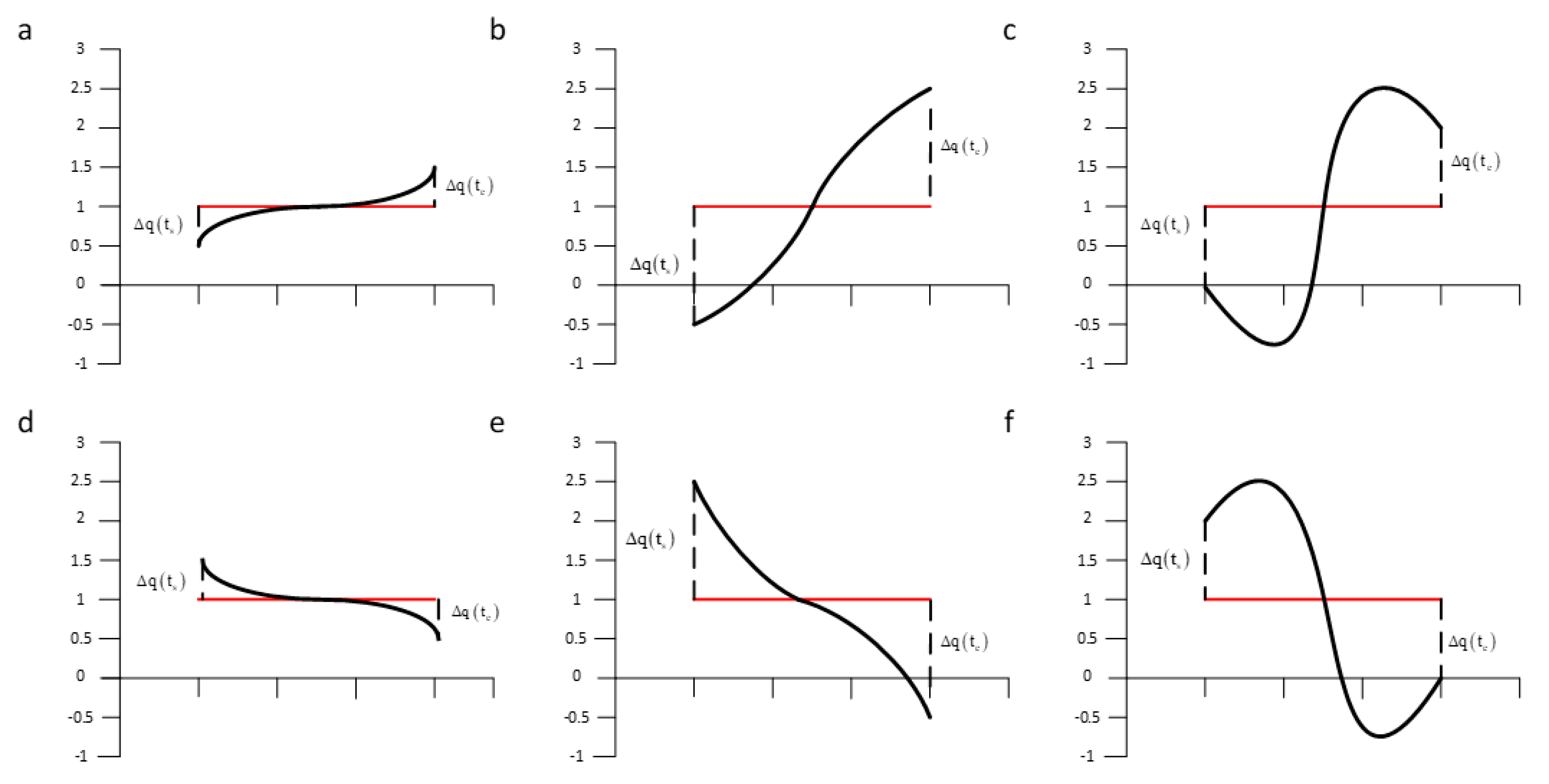
As the first to symbolize time series and can be effectively applied to time series classification, SAX has been recognized by many experts and scholars, however the shortcoming is also obviously to see. The larger w and smaller α, the more features will be lost for time series. To keep as much important information as possible, time series trend needed to be kept in the process of SAX dimensionality reduction. For example, in reference [26], some limitations of using SAX algorithm on the classification for time series were discussed. In this paper, these cases are listed separately in Figure 2.
In Figure 2, the average value of a and d, b and e, c, and f correspond to the same, but it is very clear that their time series tend to be significantly different. In order to correctly describe this difference, the author proposes using the SAX-TD method. According to the calculation rules of SAX-TD, the trend distance td (q, c) of two time series q and c is first calculated. The specific definition is as follows:
where and are the start point and end point of a time segment for the time series q and c. Respectively, the specific definition of is as follows:
will be calculated in the same way, in article the author refers to this method as the tendency of time segments.
With the SAX method description, the time series Q and C respectively represented as follows:
is a sequence symbolized by SAX, are the trend variations, and is the change of the last point.
The distance between two time series can be defined based on the trend distance as follows:
where and respectively, denote the time series Q and C, n is the length of Q and C, and w is the number of time segments. The distance between time series Q and C can be calculated by Equation (6). In this paper, the author proved that this method has a low bound to Euclidean distance, and the experimental results also showed that this method improves classification accuracy compared with ESAX.
3. SAX-BD: Boundary Distance-Based Method For Time Series
3.1. An Analysis of SAX-TD
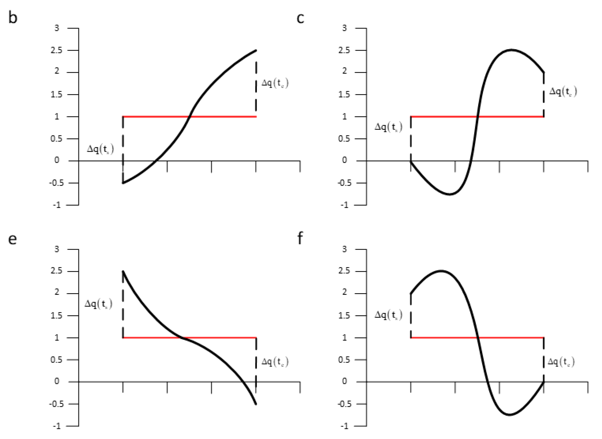
The difference between b and e, c and f can be identified by using the SAX-TD algorithm, because, for b, the trend distance is , and for the e is , the final calculation results can distinguish these time series. However, if you want to identify the difference between a and c, e and f, there is a great possibility that you will fail. The trend distance for b and c, e and f are both the same value or , according to the calculation rules of SAX-TD, they will be judged as the same time series.
3.2. Our Method SAX-BD
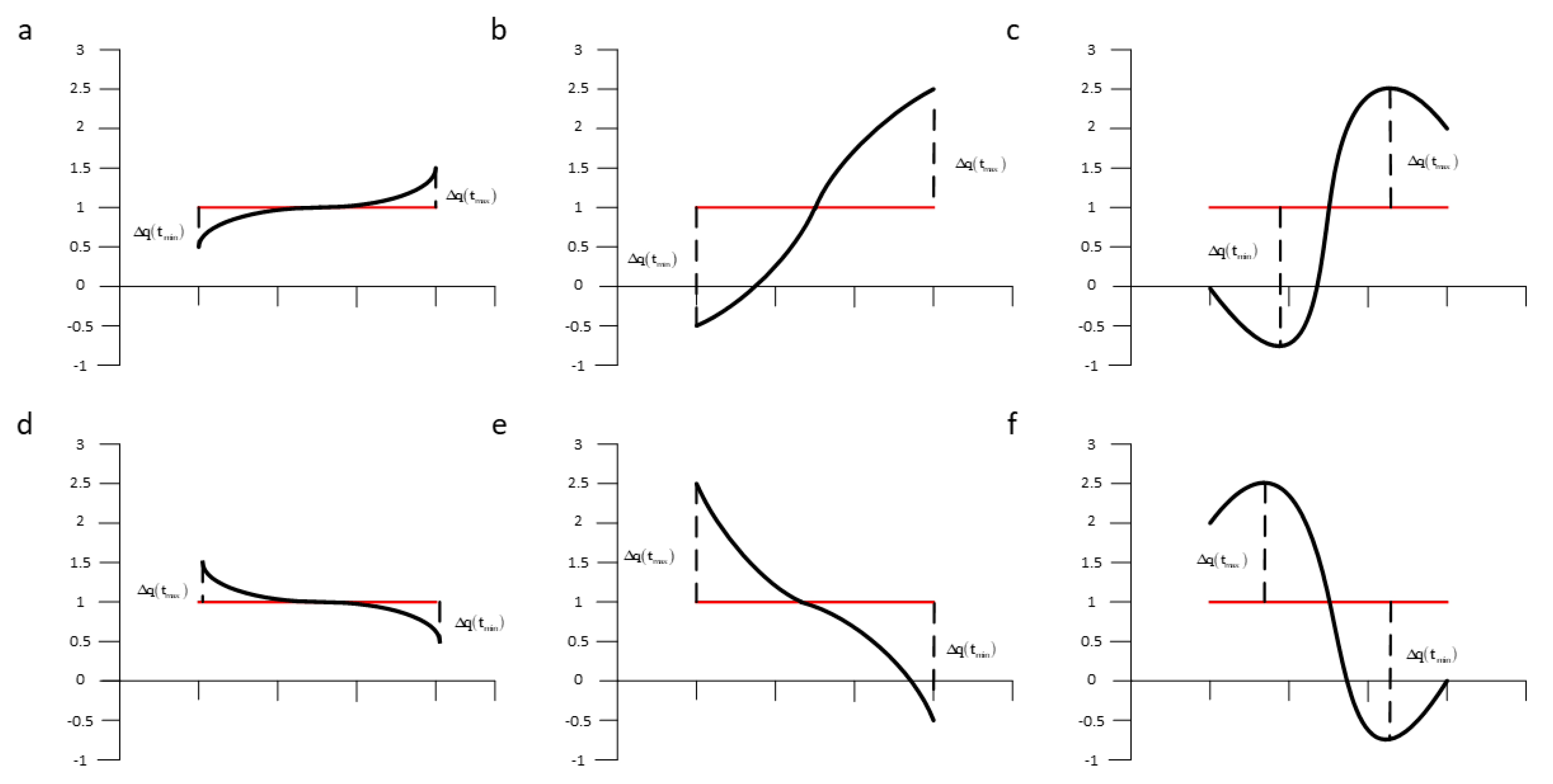
In order to solve these problems, we propose to increase the boundary distance as a new reference instead of the trend distance. The details are as follows:
From Figure 4, we can see that this method is somewhat the same as ESAX, but it is different from ESAX.
The maximum and minimum value of each time segment is the boundary. The boundary distance of c isand for f is, shown in Equations (7) and (8):
The tendency change of c calculated by SAX-BD algorithm is , and the tendency change of f is . It can be seen that our method can also distinguish well. For b and c, the distance calculated using SAX-TD is the same, but in our method, SAX-BD, the equation is not equal to 0, indicating that there is a possibility of distinction between the time series. For the cases of g and h, according to our method, it is as follows:
3.3. Difference from ESAX
In the ESAX method, the maximum, minimum, and mean values in each time segment are mapped and arranged according to the following formula:
However, for the same feature points, we did not directly map these points in the same way as the ESAX method, mainly due to the following two reasons:
Firstly, in Figure 5, if you follow these points in the ESAX method diagram, for example, for A, B, C, D, E, they will all be mapped to the same character ‘f’ for α = 6 and F, G, H will be mapped to ‘a’. We directly retain these feature points and calculate the boundary distance. At this time, the specific values of A, B, C, D, E, and F, G, H can have a better discrimination.
Secondly, if we follow the ESAX method, we can see from Equation (11) that there may be a total of 6 comparisons. In fact, according to our method, only two comparisons are needed. Since our distance measurement is consistent with SXA-TD, the low correlation between Equation (13) and Euclidean distance has also been proven in the SAX-TD paper.
Finally, time series Q and C can be expressed as follows according to our method SAX-BD:
The equation for calculating the distance between Q and C can be expressed as follows:
3.4. Lower Bound
One of the most important characteristics of the SAX is that it provides a lower bounding distance measure. Lower bound is very useful for controlling errors and speeding up the computation. Below, we will show that our proposed distance also lower bounds the Euclidean distance.
According to [19,20], we have proved that the PAA distance lower bounds the Euclidean distance as follows:
For proving the TDIST also lower bounds the Euclidean distance, we repeat some of the proofs here. Let Q and C be the means of time series Q and C respectively. We first consider only the single frame case (i.e., w = 1), Equation (14) can be rewritten as follows:
Recall that Q is the average of the time series, so can be represented in terms of . The same applies to each point in C, Equation (15) can be rewritten as follows:
Because , Recall the definition in Equation (9) and Equation (12), , we can obtain an inequality as follows (its’ obviously exists that the boundary distance in ):
Substituting Equation (16) into Equation (17), we get:
According to [20], the MINDIST lower bounds the PAA distance, that is:
where and are symbolic representations of Q and C in the original SAX, respectively. By transitivity, the following inequality is true
Recall Equation (15), this means
N frames can be obtained by applying the single-frame proof on every frame, that is
The quality of a lower bounding distance is usually measured by the tightness of lower bounding (TLB).
The value of TLB is in the range [0, 1]. The larger the TLB value, the better the quality. Recall the distance measure in Equation (13), we can obtain that which means the SAX-BD distance has a tighter lower bound than the original SAX distance.
4. Experimental Validation
In this section, we will present the results of our experimental validation. We used a stand-alone desktop computer, Inter(R) Core(TM) i5-4440 CPU @ 3.10 GHz.
Firstly, we introduce the data sets used, the comparison methods and parameter settings. Then, in order to show experimental results more conveniently, we evaluate the performances of the proposed method in terms of classification accuracy rate shown in figures and classification error rate shown in tables.
4.1. Data Sets
According to the latest time series database UCRArchive2018, in order to make the experimental results more credible, 100 data sets were obtained on the basis of removing null values in the data and show in Table 2. Each data set is divided into a training set and a testing set and a detailed documentation of the data. The datasets contain classes ranging from 2 to 60 and have the lengths of time series varying from 15 to 2844. In addition, the types of the data sets are also diverse, including image, sensor, motion, ECG, etc. [27].
4.2. Comparison Methods and Parameter Settings
We compare the result with the above-mentioned ESAX and SAX. We also compare with SAX-TD, which is another latest research improving SAX based on the trend distance. We do the evaluation on the classification task, of which the accuracy is determined by the distance measure. In this way, it is well proved that our method improves the SAX-TD method. To compare the classification accuracy, we conduct the experiments using the 1 nearest neighbor (1-NN) classifier by reading the sun’s paper [26].
To make it fairer for each method, we use the testing data to search for the best parameters w and α. For a given timeseries of length n, w and α are picked using the following criteria [28]):
For w, we search for the value from 2 up ton = 2 and double the value of w each time.
For α, we search for the value from 3 up to 10.
If two sets of parameter settings produce the same classification error rate, we choose the smaller parameters.
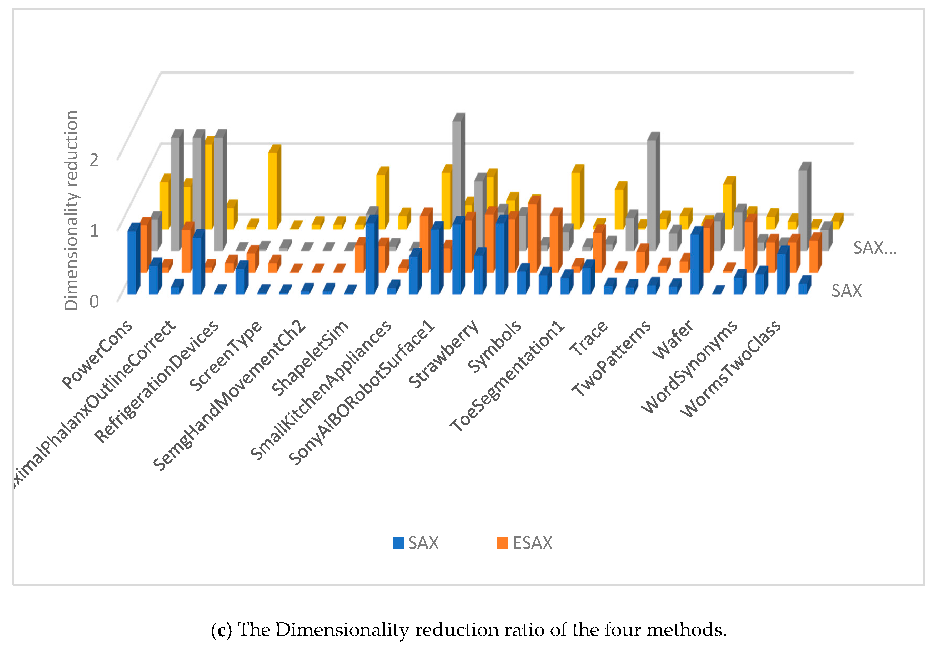
The dimensionality reduction ratios are defined as follows:
4.3. Result Analysis
To make the table fit all the data, we abbreviate SAX-TD for SAXTD and SAX-BD for SAXBD. The overall classification results are listed in Table 3, where entries with the lowest classification error rates are highlighted. SAX-BD has the lowest error in the most of the data sets (69/100), followed by SAX-TD (22/100), EU (15/100). In some cases, it performs much better than the other two methods, and even achieves a 0 classification error rate.
We use the Wilcoxon signed ranks test to test the significance of our method against other methods. The test results are displayed in Table 4. Where , and denote the numbers of data sets where the error rates of the SAX-BD are lower, larger than and equal to those of another method respectively. The p-values (the smaller a p-value, the more significant the improvement) demonstrate that our distance measure achieves a significant improvement over the other four methods on classification accuracy.
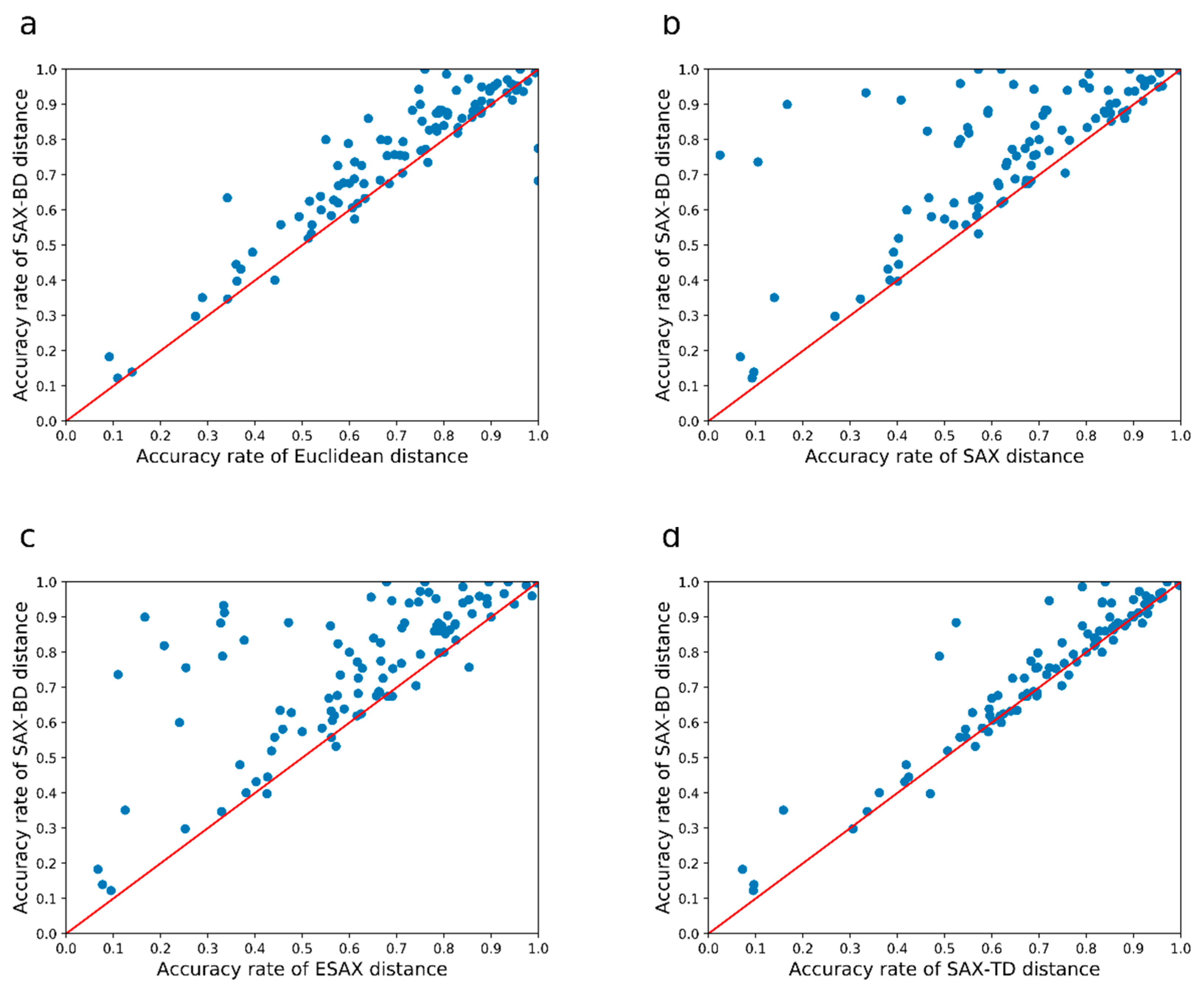
To provide a more intuitive illustration of the performance of the different measures compared in Table 3 and Table 4, we use scatter plots for pairwise comparisons. In a scatter plot, the accuracy rates of two measures under comparison are used as the x and y coordinates of a dot, where a dot represents a data set. When a dot above the diagonal line, the ‘y’ method performs better than the ‘x’ method. In addition, the further a dot is from the diagonal line, the greater the margin of an accuracy improvement. The region with more dots indicates a better method than the other.
In the following, we explain the results in Figure 6.
We illustrate the performance of our distance measure against the Euclidean distance, SAX distance, ESAX distance, SAX-TD distance in Figure 6a–d, respectively. Our method outperforms the other four methods by a large margin, both in the number of points and the distance of these points from the diagonals. From these figures, we can see that most of the points are far away from the diagonals, which indicates that our method has much lower error rates on most of the data sets.
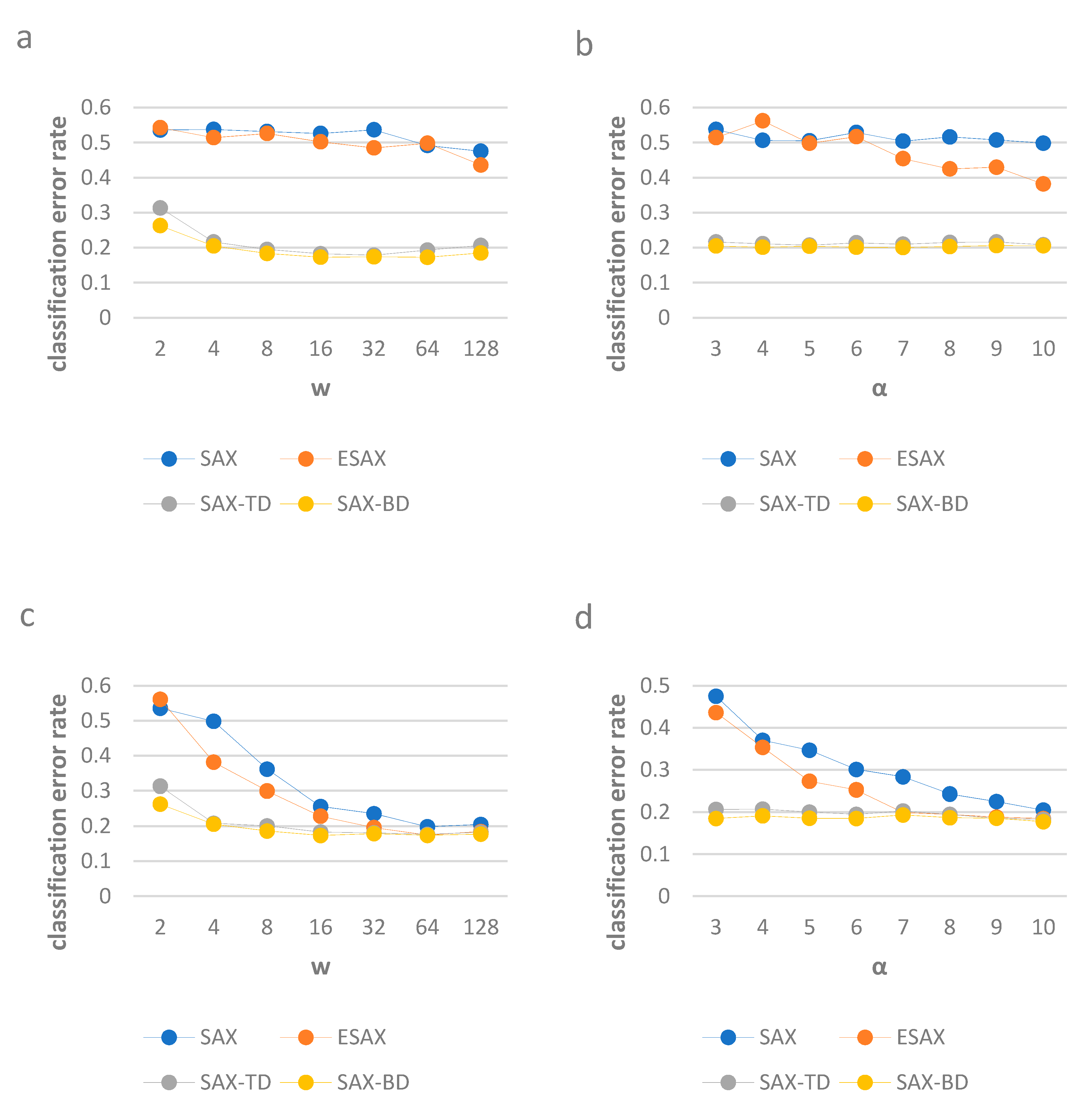
To show the continuity performance of our method and other three methods, we run the experiments on data set Yoga. We firstly compare the classification error rates with different w while α is fixed at 3, and then with different α while w is fixed at 4 (to illustrate the classification error rates using small parameters). Secondly, we use w, which varies, while α is fixed at 10, and then α varies while w is fixed at 128 (to illustrate the classification error rates using large parameters).
SAX-TD and SAX-BD has lower error rates than the other two methods when the parameters are small and large, SAX-BD has lower error rates than the SAX-TD. The results are shown in Figure 7.
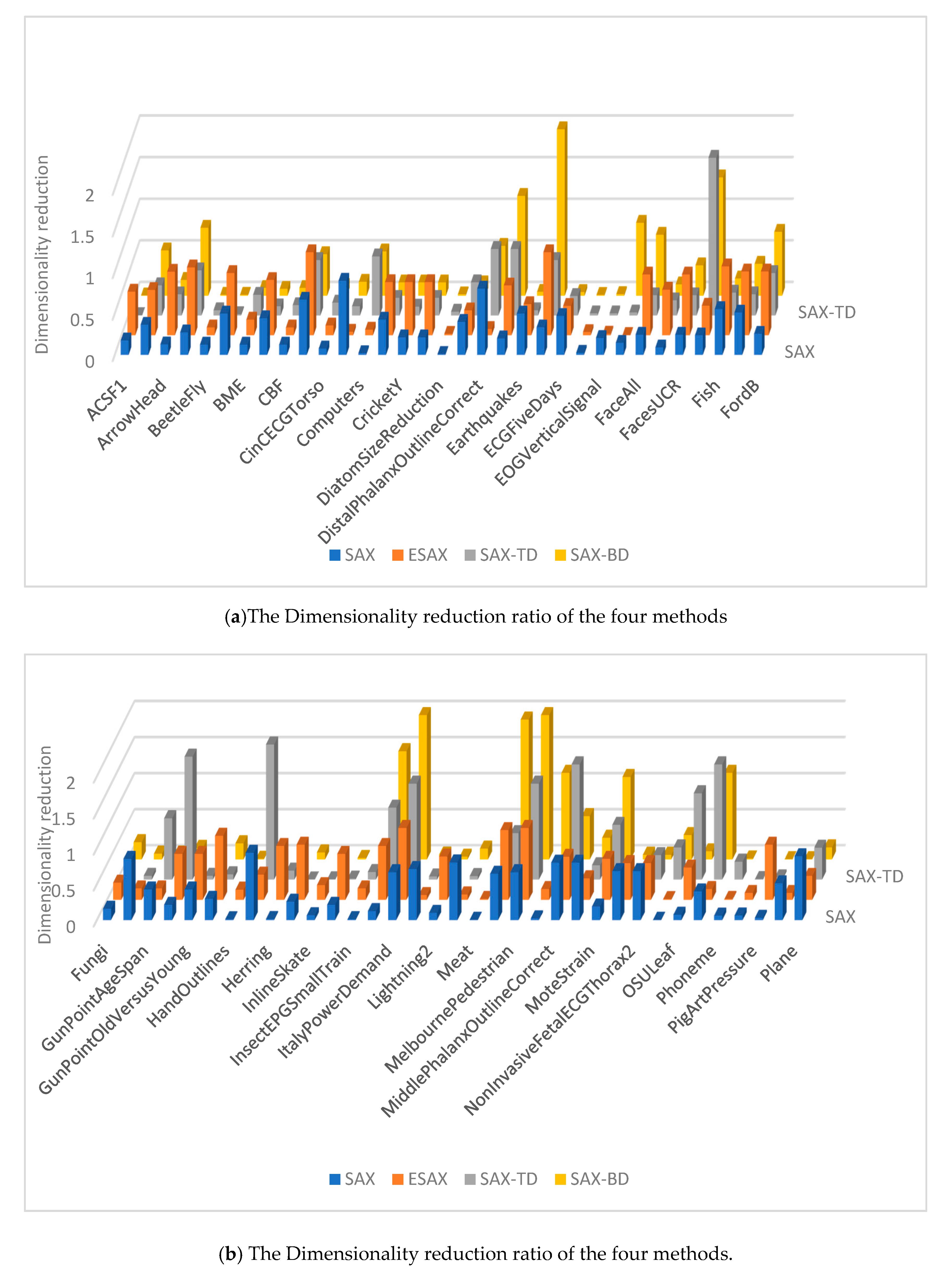
The dimensionality reduction ratios are calculated using the w when the four methods achieve their smallest classification error rates on each data set, shown in Figure 8. The SAX-TD and SAX-BD representation use more values than SAX, SAX-TD use fewer values than ESAX. In fact, our method has a low dimensionality reduction ratio in majority datasets, and even uses fewer values than SAX-TD.
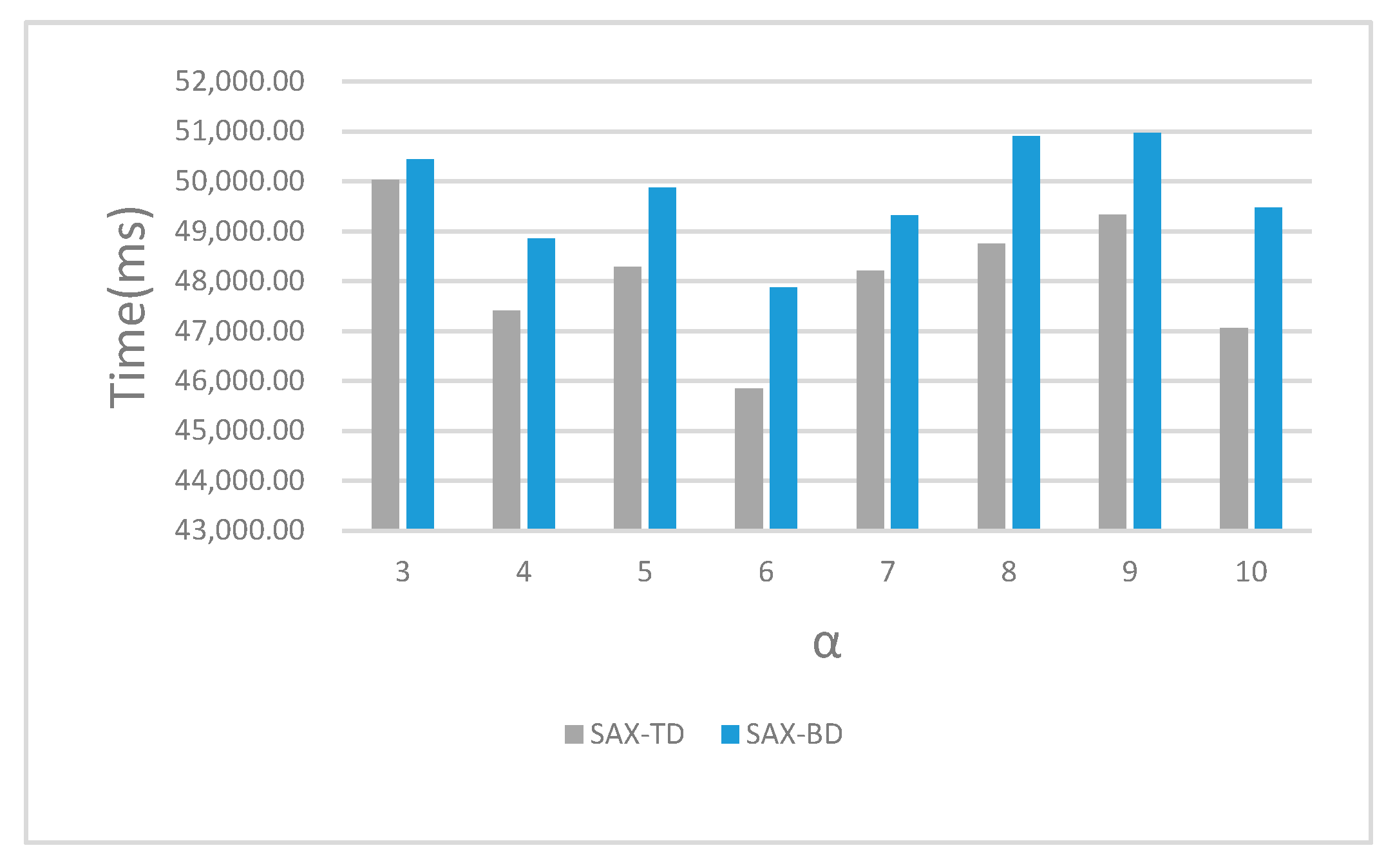
We also recorded the running time of SAX-TD and SAX-BD with different α from 3 to 10 shown in Figure 9. The experimental results indicated that we have made a greater improvement at the cost of only a little time, and that’s well worth it.
5. Conclusions
Our proposed SAX-BD algorithm uses the boundary distance as a new distance metric to obtain a new time series representation. We analyze some cases that ESAX and SAX-TD cannot solve, and it is known that the classification accuracy of ESAX algorithm is not as good as SAX-TD. We combine the advantages of these two methods, analyzing and deriving our method as an extension of these two methods. We also proved that our improved distance measure not only keeps a lower-bound to the Euclidean distance, but also has a low dimensionality reduction ratio in majority datasets. In terms of the expression complexity of time series, our algorithm SAX-BD and ESAX algorithm are three times more than SAX, and two times more than SAX-TD. However, in terms of running time, we spend just a little more. In terms of the classification accuracy, we have improved this a lot, that means a good compromise has made between dimensional reduction and classification accuracy. For future work, we intend to change our original algorithm to make time advantage.
Author Contributions
Methodology, Z.H. and S.L.; Project administration, Z.H.; Software, H.Z.; Writing—review & editing, X.M. All authors have read and agreed to the published version of the manuscript.
Funding
The work described in this paper was supported by the National Natural Science Foundation of China (41972306, U1711267, 41572314) and the geo-disaster data processing and intelligent monitoring project.
Conflicts of Interest
The authors declare no conflict of interest.
References
- Abanda, A.; Mori, U.; Lozano, J.A. A review on distance based time series classification. Data Min. Knowl. Discov. 2018, 33, 378–412. [Google Scholar] [CrossRef] [Green Version]
- Keogh, E.J.; Kasetty, S. On the Need for Time Series Data Mining Benchmarks: A Survey and Empirical Demonstration. Data Min. Knowl. Discov. 2003, 7, 349–371. [Google Scholar] [CrossRef]
- Vlachos, M.; Kollios, G.; Gunopulos, D. Discovering similar multidimensional trajectories. In Proceedings of the 18th International Conference on Data Engineering, San Jose, CA, USA, 26 Febuary–1 March 2002; p. 673. [Google Scholar]
- Lonardi, J.; Patel, P. Finding motifs in time series. In Proceedings of the 2nd Workshop on Temporal Data Mining, Washington, DC, USA, 24–27 August 2002. [Google Scholar]
- Keogh, E.; Lonardi, S.; Chiu, B.Y. Finding surprising patterns in a time series database in linear time and space. In Proceedings of the Eighth ACM SIGKDD International Conference on Knowledge Discovery and Data Mining, Edmonton, AB, Canada, 23–25 July 2002. [Google Scholar]
- Kalpakis, K.; Gada, D.; Puttagunta, V. Distance measures for effective clustering of ARIMA time-series. In Proceedings of the 2001 IEEE International Conference on Data Mining, San Jose, CA, USA, 29 November–2 December 2001; pp. 273–280. [Google Scholar]
- Huang, Y.-W.; Yu, P.S. Adaptive query processing for time-series data. In Proceedings of the Fifth ACM SIGKDD International Conference on Knowledge Discovery and Data Mining—KDD ’99, San Diego, CA, USA, 15–18 August 1999; pp. 282–286. [Google Scholar]
- Chan, K.-P.; Fu, A.W.-C. Efficient time series matching by wavelets. In Proceedings of the 15th International Conference on Data Engineering (Cat. No.99CB36337), Sydney, Australia, 23–26 March 1999; pp. 126–133. [Google Scholar]
- Dasgupta, D.; Forrest, S. Novelty detection in time series data using ideas from immunology. In Proceedings of the International Conference on Intelligent Systems, Ahmedabad, Indian, 15–16 November 1996. [Google Scholar]
- Xing, Z.; Pei, J.; Keogh, E. A brief survey on sequence classification. ACM SIGKDD Explor. Newsl. 2010, 12, 40–48. [Google Scholar] [CrossRef]
- Faloutsos, C.; Ranganathan, M.; Manolopoulos, Y. Fast subsequence matching in time-series databases. ACM Sigmod Rec. 1994, 23, 419–429. [Google Scholar] [CrossRef] [Green Version]
- Popivanov, I.; Miller, R. Similarity search over time-series data using wavelets. In Proceedings of the 18th International Conference on Data Engineering, Washington, DC, USA, 26 February–1 March 2002. [Google Scholar]
- Korn, F.; Jagadish, H.V.; Faloutsos, C. Efficiently supporting ad hoc queries in large datasets of time sequences. ACM Sigmod Rec. 1997, 26, 289–300. [Google Scholar] [CrossRef]
- Bagnall, A.; Janacek, G. A Run Length Transformation for Discriminating Between Auto Regressive Time Series. J. Classif. 2013, 31, 154–178. [Google Scholar] [CrossRef] [Green Version]
- Corduas, M.; Piccolo, D. Time series clustering and classification by the autoregressive metric. Comput. Stat. Data Anal. 2008, 52, 1860–1872. [Google Scholar] [CrossRef]
- Smyth, P. Clustering sequences with hidden Markov models. In Proceedings of the Advances in Neural Information Processing Systems, Curitiba, Brazil, 2–5 November 1997. [Google Scholar]
- Berndt, D.J.; Clifford, J. Using dynamic time warping to find patterns in time series. In Proceedings of the KDD Workshop, Seattle, WA, USA, 31 July 1994. [Google Scholar]
- Keogh, E.J.; Chakrabarti, K.; Pazzani, M.J.; Mehrotra, S. Dimensionality Reduction for Fast Similarity Search in Large Time Series Databases. Knowl. Inf. Syst. 2001, 3, 263–286. [Google Scholar] [CrossRef]
- Hellerstein, J.M.; Koutsoupias, E.; Papadimitriou, C.H. On the analysis of indexing schemes. In Proceedings of the Sixteenth ACM SIGACT-SIGMOD-SIGART Symposium on Principles of Database Systems—PODS ’97, Tucson, AZ, USA, 12–14 May 1997. [Google Scholar]
- Lin, J.; Keogh, E.; Lonardi, S.; Chiu, B. A symbolic representation of time series, with implications for streaming algorithms. In Proceedings of the 8th ACM SIGMOD Workshop on Research Issues in Data Mining and Knowledge Discovery, San Diego, CA, USA, 13 June 2003. [Google Scholar]
- Tayebi, H.; Krishnaswamy, S.; Waluyo, A.B.; Sinha, A.; Abouelhoda, M.; Waluyo, A.B.; Sinha, A. RA-SAX: Resource-Aware Symbolic Aggregate Approximation for Mobile ECG Analysis. In Proceedings of the 2011 IEEE 12th International Conference on Mobile Data Management, Lulea, Sweden, 6–9 June 2011; Volume 1, pp. 289–290. [Google Scholar]
- Canelas, A.; Neves, R.F.; Horta, N. A new SAX-GA methodology applied to investment strategies optimization. In Proceedings of the Fourteenth International Conference on Genetic and Evolutionary Computation Conference Companion—GECCO Companion ’12, Philadelphia, PA, USA, 7–11 July 2012; pp. 1055–1062. [Google Scholar]
- Rakthanmanon, T.; Keogh, E. Fast shapelets: A scalable algorithm for discovering time series shapelets. In Proceedings of the 2013 SIAM International Conference on Data Mining, Austin, TX, USA, 2–4 May 2013. [Google Scholar]
- Zheng, Y.; Liu, Q.; Chen, E.; Ge, Y.; Zhao, J.L. Time Series Classification Using Multi-Channels Deep Convolutional Neural Networks. In Proceedings of the Lecture Notes in Computer Science, Leipzig, Germany, 22–26 June 2014; Springer Science and Business Media LLC: Macau, China, 2014; pp. 298–310. [Google Scholar]
- Lkhagva, B.; Suzuki, Y.; Kawagoe, K. New Time Series Data Representation ESAX for Financial Applications. In Proceedings of the 22nd International Conference on Data Engineering Workshops (ICDEW’06), Atlanta, GA, USA, 3–7 April 2006; p. 115. [Google Scholar]
- Sun, Y.; Li, J.; Liu, J.; Sun, B.; Chow, C. An improvement of symbolic aggregate approximation distance measure for time series. Neurocomputing 2014, 138, 189–198. [Google Scholar] [CrossRef]
- Dau, H.A.; Bagnall, A.; Kamgar, K.; Yeh, C.-C.M.; Zhu, Y.; Gharghabi, S.; Ratanamahatana, C.A.; Keogh, E. The UCR time series archive. IEEE/CAA J. Autom. Sin. 2019, 6, 1293–1305. [Google Scholar] [CrossRef]
- Lin, J.; Keogh, E.; Wei, L.; Lonardi, S. Experiencing SAX: A novel symbolic representation of time series. Data Min. Knowl. Discov. 2007, 15, 107–144. [Google Scholar] [CrossRef] [Green Version]
Figure 1.
Financial time series A and B have the same SAX symbolic representation ‘decfdb’ in the same condition where the length of time series is 30, the number of segments is 6 and the size of symbols is 6. However, they are different time series.
Figure 1.
Financial time series A and B have the same SAX symbolic representation ‘decfdb’ in the same condition where the length of time series is 30, the number of segments is 6 and the size of symbols is 6. However, they are different time series.

Figure 2.
Several typical segments with the same average value but different trends [26]. Segment a and d, b and e, c and f are in opposite directions while all in same mean value.
Figure 2.
Several typical segments with the same average value but different trends [26]. Segment a and d, b and e, c and f are in opposite directions while all in same mean value.

Figure 3.
Several typical segments with the same average value and same trends but different boundary distance. Segment b and c, e and f with the same SAX representation and trend distance while they are different segments.
Figure 3.
Several typical segments with the same average value and same trends but different boundary distance. Segment b and c, e and f with the same SAX representation and trend distance while they are different segments.

Figure 4.
Several typical segments with the same average value but boundary distance. Segment a and d, b and e, c and f are in opposite directions while all in same mean value. The trend distance is replaced by boundary distance.
Figure 4.
Several typical segments with the same average value but boundary distance. Segment a and d, b and e, c and f are in opposite directions while all in same mean value. The trend distance is replaced by boundary distance.

Figure 5.
Time series represented as ‘adfeeffcaefffdaabc’ by ESAX [25]. Where the length of time series is 30, the number of segments is 6 and the size of symbols is 6. The capital letters A–H represent the maximum and minimum values in every segment.
Figure 5.
Time series represented as ‘adfeeffcaefffdaabc’ by ESAX [25]. Where the length of time series is 30, the number of segments is 6 and the size of symbols is 6. The capital letters A–H represent the maximum and minimum values in every segment.

Figure 6.
The SAX-BD algorithm is compared with other algorithms for accuracy. (a–d) represents a comparison between SAX-BD with Euclidean, SAX, ESAX, SAX-TD. The more dots above the red slash, the better performs of SAX-BD.
Figure 6.
The SAX-BD algorithm is compared with other algorithms for accuracy. (a–d) represents a comparison between SAX-BD with Euclidean, SAX, ESAX, SAX-TD. The more dots above the red slash, the better performs of SAX-BD.

Figure 7.
The classification error rates of SAX, ESAX, SAX-TD and SAX-BD with different parameters w and α. For (a), on Gun-Point, w varies while α is fixed at 3, for (b), on Gun-Point, varies while w is fixed at 4. For (c), on Yoga, w varies while α is fixed at 10, for (d), on Yoga, varies while w is fixed at 128.

Figure 8.
Dimensionality reduction ratio of the four methods.


Figure 9.
The running time of different methods with different values of α.


Table 1.
A lookup table for breakpoints with the alphabet size from 3 to 10.
| 3 | 2 | 5 | 6 | 7 | 8 | 9 | 10 | |
|---|---|---|---|---|---|---|---|---|
| −0.43 | −0.67 | −0.84 | −0.97 | −1.07 | −1.15 | −1.22 | −1.28 | |
| −0.43 | 0 | −0.25 | −0.43 | −0.57 | −0.67 | −0.76 | −0.84 | |
| 0.67 | 0.25 | 0 | −0.18 | −0.32 | −0.43 | −0.52 | ||
| 0.84 | 0.43 | 0.18 | 0 | −0.14 | −0.25 | |||
| 0.97 | 0.57 | 0.32 | 0.14 | 0 | ||||
| 1.07 | 0.67 | 0.43 | 0.25 | |||||
| 1.15 | 0.76 | 0.52 | ||||||
| 1.22 | 0.84 | |||||||
| 1.28 |
Table 2.
100 different types of time series datasets.
| ID | Type | Name | Train | Test | Class | Length |
|---|---|---|---|---|---|---|
| 1 | Device | ACSF1 | 100 | 100 | 10 | 1460 |
| 2 | Image | Adiac | 390 | 391 | 37 | 176 |
| 3 | Image | ArrowHead | 36 | 175 | 3 | 251 |
| 4 | Spectro | Beef | 30 | 30 | 5 | 470 |
| 5 | Image | BeetleFly | 20 | 20 | 2 | 512 |
| 6 | Image | BirdChicken | 20 | 20 | 2 | 512 |
| 7 | Simulated | BME | 30 | 150 | 3 | 128 |
| 8 | Sensor | Car | 60 | 60 | 4 | 577 |
| 9 | Simulated | CBF | 30 | 900 | 3 | 128 |
| 10 | Traffic | Chinatown | 20 | 343 | 2 | 24 |
| 11 | Sensor | CinCECGTorso | 40 | 1380 | 4 | 1639 |
| 12 | Spectro | Coffee | 28 | 28 | 2 | 286 |
| 13 | Device | Computers | 250 | 250 | 2 | 720 |
| 14 | Motion | CricketX | 390 | 390 | 12 | 300 |
| 15 | Motion | CricketY | 390 | 390 | 12 | 300 |
| 16 | Motion | CricketZ | 390 | 390 | 12 | 300 |
| 17 | Image | DiatomSizeReduction | 16 | 306 | 4 | 345 |
| 18 | Image | DistalPhalanxOutlineAgeGroup | 400 | 139 | 3 | 80 |
| 19 | Image | DistalPhalanxOutlineCorrect | 600 | 276 | 2 | 80 |
| 20 | Image | DistalPhalanxTW | 400 | 139 | 6 | 80 |
| 21 | Sensor | Earthquakes | 322 | 139 | 2 | 512 |
| 22 | ECG | ECG200 | 100 | 100 | 2 | 96 |
| 23 | ECG | ECGFiveDays | 23 | 861 | 2 | 136 |
| 24 | EOG | EOGHorizontalSignal | 362 | 362 | 12 | 1250 |
| 25 | EOG | EOGVerticalSignal | 362 | 362 | 12 | 1250 |
| 26 | Spectro | EthanolLevel | 504 | 500 | 4 | 1751 |
| 27 | Image | FaceAll | 560 | 1690 | 14 | 131 |
| 28 | Image | FaceFour | 24 | 88 | 4 | 350 |
| 29 | Image | FacesUCR | 200 | 2050 | 14 | 131 |
| 30 | Image | FiftyWords | 450 | 455 | 50 | 270 |
| 31 | Image | Fish | 175 | 175 | 7 | 463 |
| 32 | Sensor | FordA | 3601 | 1320 | 2 | 500 |
| 33 | Sensor | FordB | 3636 | 810 | 2 | 500 |
| 34 | HRM | Fungi | 18 | 186 | 18 | 201 |
| 35 | Motion | GunPoint | 50 | 150 | 2 | 150 |
| 36 | Motion | GunPointAgeSpan | 135 | 316 | 2 | 150 |
| 37 | Motion | GunPointMaleVersusFemale | 135 | 316 | 2 | 150 |
| 38 | Motion | GunPointOldVersusYoung | 136 | 315 | 2 | 150 |
| 39 | Spectro | Ham | 109 | 105 | 2 | 431 |
| 40 | Image | HandOutlines | 1000 | 370 | 2 | 2709 |
| 41 | Motion | Haptics | 155 | 308 | 5 | 1092 |
| 42 | Image | Herring | 64 | 64 | 2 | 512 |
| 43 | Device | HouseTwenty | 40 | 119 | 2 | 2000 |
| 44 | Motion | InlineSkate | 100 | 550 | 7 | 1882 |
| 45 | EPG | InsectEPGRegularTrain | 62 | 249 | 3 | 601 |
| 46 | EPG | InsectEPGSmallTrain | 17 | 249 | 3 | 601 |
| 47 | Sensor | InsectWingbeatSound | 220 | 1980 | 11 | 256 |
| 48 | Sensor | ItalyPowerDemand | 67 | 1029 | 2 | 24 |
| 49 | Device | LargeKitchenAppliances | 375 | 375 | 3 | 720 |
| 50 | Sensor | Lightning2 | 60 | 61 | 2 | 637 |
| 51 | Sensor | Lightning7 | 70 | 73 | 7 | 319 |
| 52 | Spectro | Meat | 60 | 60 | 3 | 448 |
| 53 | Image | MedicalImages | 381 | 760 | 10 | 99 |
| 54 | Traffic | MelbournePedestrian | 1194 | 2439 | 10 | 24 |
| 55 | Image | MiddlePhalanxOutlineAgeGroup | 400 | 154 | 3 | 80 |
| 56 | Image | MiddlePhalanxOutlineCorrect | 600 | 291 | 2 | 80 |
| 57 | Image | MiddlePhalanxTW | 399 | 154 | 6 | 80 |
| 58 | Sensor | MoteStrain | 20 | 1252 | 2 | 84 |
| 59 | ECG | NonInvasiveFetalECGThorax1 | 1800 | 1965 | 42 | 750 |
| 60 | ECG | NonInvasiveFetalECGThorax2 | 1800 | 1965 | 42 | 750 |
| 61 | Spectro | OliveOil | 30 | 30 | 4 | 570 |
| 62 | Image | OSULeaf | 200 | 242 | 6 | 427 |
| 63 | Image | PhalangesOutlinesCorrect | 1800 | 858 | 2 | 80 |
| 64 | Sensor | Phoneme | 214 | 1896 | 39 | 1024 |
| 65 | Hemodynamics | PigAirwayPressure | 104 | 208 | 52 | 2000 |
| 66 | Hemodynamics | PigArtPressure | 104 | 208 | 52 | 2000 |
| 67 | Hemodynamics | PigCVP | 104 | 208 | 52 | 2000 |
| 68 | Sensor | Plane | 105 | 105 | 7 | 144 |
| 69 | Power | PowerCons | 180 | 180 | 2 | 144 |
| 70 | Image | ProximalPhalanxOutlineAgeGroup | 400 | 205 | 3 | 80 |
| 71 | Image | ProximalPhalanxOutlineCorrect | 600 | 291 | 2 | 80 |
| 72 | Image | ProximalPhalanxTW | 400 | 205 | 6 | 80 |
| 73 | Device | RefrigerationDevices | 375 | 375 | 3 | 720 |
| 74 | Spectrum | Rock | 20 | 50 | 4 | 2844 |
| 75 | Device | ScreenType | 375 | 375 | 3 | 720 |
| 76 | Spectrum | SemgHandGenderCh2 | 300 | 600 | 2 | 1500 |
| 77 | Spectrum | SemgHandMovementCh2 | 450 | 450 | 6 | 1500 |
| 78 | Spectrum | SemgHandSubjectCh2 | 450 | 450 | 5 | 1500 |
| 79 | Simulated | ShapeletSim | 20 | 180 | 2 | 500 |
| 80 | Image | ShapesAll | 600 | 600 | 60 | 512 |
| 81 | Device | SmallKitchenAppliances | 375 | 375 | 3 | 720 |
| 82 | Simulated | SmoothSubspace | 150 | 150 | 3 | 15 |
| 83 | Sensor | SonyAIBORobotSurface1 | 20 | 601 | 2 | 70 |
| 84 | Sensor | SonyAIBORobotSurface2 | 27 | 953 | 2 | 65 |
| 85 | Spectro | Strawberry | 613 | 370 | 2 | 235 |
| 86 | Image | SwedishLeaf | 500 | 625 | 15 | 128 |
| 87 | Image | Symbols | 25 | 995 | 6 | 398 |
| 88 | Simulated | SyntheticControl | 300 | 300 | 6 | 60 |
| 89 | Motion | ToeSegmentation1 | 40 | 228 | 2 | 277 |
| 90 | Motion | ToeSegmentation2 | 36 | 130 | 2 | 343 |
| 91 | Sensor | Trace | 100 | 100 | 4 | 275 |
| 92 | ECG | TwoLeadECG | 23 | 1139 | 2 | 82 |
| 93 | Simulated | TwoPatterns | 1000 | 4000 | 4 | 128 |
| 94 | Simulated | UMD | 36 | 144 | 3 | 150 |
| 95 | Sensor | Wafer | 1000 | 6164 | 2 | 152 |
| 96 | Spectro | Wine | 57 | 54 | 2 | 234 |
| 97 | Image | WordSynonyms | 267 | 638 | 25 | 270 |
| 98 | Motion | Worms | 181 | 77 | 5 | 900 |
| 99 | Motion | WormsTwoClass | 181 | 77 | 2 | 900 |
| 100 | Image | Yoga | 300 | 3000 | 2 | 426 |
Table 3.
1-NN classification error rates of different methods.
| ID | EU Error | SAX Error | SAX w | SAX Ratio | SAX α | ESAX Error | ESAX w | ESAX Ratio | ESAX α | SAXTD Error | SAXTD w | SAXTD Ratio | SAXTD α | SAXBD Error | SAXBD w | SAXBD Ratio | SAXBD α |
|---|---|---|---|---|---|---|---|---|---|---|---|---|---|---|---|---|---|
| 1 | 0.460 | 0.580 | 256 | 0.175 | 8 | 0.760 | 256 | 0.526 | 3 | 0.380 | 4 | 0.005 | 3 | 0.400 | 2 | 0.004 | 3 |
| 2 | 0.389 | 0.895 | 64 | 0.364 | 9 | 0.890 | 32 | 0.545 | 7 | 0.284 | 32 | 0.364 | 3 | 0.263 | 32 | 0.545 | 4 |
| 3 | 0.200 | 0.309 | 32 | 0.127 | 10 | 0.349 | 64 | 0.765 | 10 | 0.183 | 32 | 0.255 | 3 | 0.160 | 16 | 0.191 | 5 |
| 4 | 0.333 | 0.467 | 128 | 0.272 | 7 | 0.400 | 128 | 0.817 | 7 | 0.167 | 128 | 0.545 | 4 | 0.200 | 128 | 0.817 | 6 |
| 5 | 0.250 | 0.150 | 64 | 0.125 | 4 | 0.100 | 16 | 0.094 | 4 | 0.150 | 16 | 0.063 | 5 | 0.100 | 2 | 0.012 | 3 |
| 6 | 0.450 | 0.300 | 256 | 0.500 | 4 | 0.200 | 128 | 0.750 | 5 | 0.200 | 4 | 0.016 | 4 | 0.200 | 2 | 0.012 | 3 |
| 7 | 0.173 | 0.153 | 16 | 0.125 | 7 | 0.160 | 8 | 0.188 | 7 | 0.147 | 16 | 0.250 | 3 | 0.060 | 4 | 0.094 | 4 |
| 8 | 0.267 | 0.283 | 256 | 0.444 | 10 | 0.283 | 128 | 0.666 | 6 | 0.133 | 32 | 0.111 | 4 | 0.117 | 16 | 0.083 | 3 |
| 9 | 0.148 | 0.084 | 16 | 0.125 | 8 | 0.250 | 4 | 0.094 | 9 | 0.088 | 8 | 0.125 | 5 | 0.027 | 4 | 0.094 | 4 |
| 10 | 0.058 | 0.467 | 16 | 0.667 | 7 | 0.125 | 8 | 1.000 | 7 | 0.041 | 8 | 0.667 | 3 | 0.041 | 4 | 0.500 | 3 |
| 11 | 0.103 | 0.097 | 128 | 0.078 | 9 | 0.108 | 64 | 0.117 | 10 | 0.072 | 128 | 0.156 | 9 | 0.062 | 64 | 0.117 | 8 |
| 12 | 0.000 | 0.429 | 256 | 0.895 | 4 | 0.321 | 4 | 0.042 | 6 | 0.000 | 16 | 0.112 | 3 | 0.000 | 16 | 0.168 | 3 |
| 13 | 0.424 | 0.480 | 16 | 0.022 | 6 | 0.432 | 16 | 0.067 | 4 | 0.404 | 256 | 0.711 | 3 | 0.380 | 128 | 0.533 | 3 |
| 14 | 0.423 | 0.385 | 128 | 0.427 | 9 | 0.444 | 64 | 0.640 | 10 | 0.400 | 32 | 0.213 | 6 | 0.331 | 16 | 0.160 | 5 |
| 15 | 0.433 | 0.441 | 64 | 0.213 | 8 | 0.523 | 64 | 0.640 | 8 | 0.441 | 16 | 0.107 | 7 | 0.372 | 16 | 0.160 | 6 |
| 16 | 0.413 | 0.387 | 64 | 0.213 | 10 | 0.426 | 64 | 0.640 | 10 | 0.387 | 32 | 0.213 | 6 | 0.323 | 16 | 0.160 | 7 |
| 17 | 0.065 | 0.062 | 4 | 0.012 | 6 | 0.232 | 2 | 0.017 | 4 | 0.039 | 8 | 0.046 | 4 | 0.029 | 2 | 0.017 | 3 |
| 18 | 0.374 | 0.317 | 32 | 0.400 | 4 | 0.381 | 8 | 0.300 | 4 | 0.331 | 16 | 0.400 | 4 | 0.273 | 4 | 0.150 | 3 |
| 19 | 0.283 | 0.348 | 64 | 0.800 | 6 | 0.308 | 2 | 0.075 | 8 | 0.264 | 32 | 0.800 | 4 | 0.246 | 16 | 0.600 | 4 |
| 20 | 0.367 | 0.432 | 16 | 0.200 | 6 | 0.439 | 16 | 0.600 | 9 | 0.360 | 32 | 0.800 | 4 | 0.367 | 32 | 1.200 | 5 |
| 21 | 0.288 | 0.245 | 256 | 0.500 | 6 | 0.259 | 64 | 0.375 | 5 | 0.252 | 16 | 0.063 | 3 | 0.295 | 8 | 0.047 | 3 |
| 22 | 0.120 | 0.080 | 32 | 0.333 | 6 | 0.140 | 32 | 1.000 | 5 | 0.070 | 32 | 0.667 | 4 | 0.090 | 64 | 2.000 | 5 |
| 23 | 0.203 | 0.114 | 64 | 0.471 | 8 | 0.211 | 16 | 0.353 | 8 | 0.081 | 16 | 0.235 | 4 | 0.117 | 2 | 0.044 | 3 |
| 24 | 0.558 | 0.616 | 32 | 0.026 | 9 | 0.619 | 16 | 0.038 | 8 | 0.638 | 16 | 0.026 | 4 | 0.599 | 4 | 0.010 | 6 |
| 25 | 0.638 | 0.599 | 256 | 0.205 | 9 | 0.575 | 8 | 0.019 | 8 | 0.530 | 16 | 0.026 | 4 | 0.602 | 8 | 0.019 | 6 |
| 26 | 0.726 | 0.732 | 256 | 0.146 | 5 | 0.748 | 2 | 0.003 | 3 | 0.694 | 32 | 0.037 | 4 | 0.702 | 512 | 0.877 | 4 |
| 27 | 0.286 | 0.320 | 32 | 0.244 | 9 | 0.250 | 32 | 0.733 | 8 | 0.227 | 16 | 0.244 | 5 | 0.206 | 32 | 0.733 | 3 |
| 28 | 0.216 | 0.159 | 32 | 0.091 | 8 | 0.205 | 64 | 0.549 | 9 | 0.136 | 32 | 0.183 | 5 | 0.125 | 16 | 0.137 | 3 |
| 29 | 0.231 | 0.252 | 32 | 0.244 | 10 | 0.334 | 32 | 0.733 | 10 | 0.251 | 16 | 0.244 | 9 | 0.173 | 16 | 0.366 | 5 |
| 30 | 0.369 | 0.327 | 64 | 0.237 | 9 | 0.319 | 32 | 0.356 | 8 | 0.334 | 256 | 1.896 | 7 | 0.325 | 128 | 1.422 | 5 |
| 31 | 0.217 | 0.451 | 256 | 0.553 | 8 | 0.623 | 128 | 0.829 | 8 | 0.143 | 64 | 0.276 | 4 | 0.166 | 32 | 0.207 | 5 |
| 32 | 0.335 | 0.327 | 256 | 0.512 | 7 | 0.336 | 128 | 0.768 | 8 | 0.304 | 64 | 0.256 | 3 | 0.315 | 64 | 0.384 | 3 |
| 33 | 0.394 | 0.428 | 128 | 0.256 | 6 | 0.436 | 128 | 0.768 | 6 | 0.399 | 128 | 0.512 | 5 | 0.394 | 128 | 0.768 | 5 |
| 34 | 0.161 | 0.118 | 32 | 0.159 | 6 | 0.210 | 16 | 0.239 | 7 | 0.172 | 16 | 0.159 | 3 | 0.140 | 16 | 0.239 | 3 |
| 35 | 0.087 | 0.207 | 128 | 0.853 | 5 | 0.013 | 8 | 0.160 | 6 | 0.073 | 4 | 0.053 | 5 | 0.040 | 4 | 0.080 | 5 |
| 36 | 0.032 | 0.111 | 64 | 0.427 | 8 | 0.051 | 8 | 0.160 | 7 | 0.076 | 64 | 0.853 | 3 | 0.063 | 4 | 0.080 | 4 |
| 37 | 0.006 | 0.044 | 32 | 0.213 | 9 | 0.025 | 32 | 0.640 | 9 | 0.003 | 128 | 1.707 | 3 | 0.009 | 8 | 0.160 | 3 |
| 38 | 0.000 | 0.108 | 64 | 0.427 | 9 | 0.063 | 32 | 0.640 | 9 | 0.000 | 4 | 0.053 | 3 | 0.000 | 2 | 0.040 | 3 |
| 39 | 0.400 | 0.324 | 128 | 0.297 | 7 | 0.343 | 128 | 0.891 | 6 | 0.305 | 16 | 0.074 | 4 | 0.324 | 32 | 0.223 | 4 |
| 40 | 0.138 | 0.162 | 32 | 0.012 | 7 | 0.176 | 128 | 0.142 | 8 | 0.130 | 8 | 0.006 | 4 | 0.119 | 8 | 0.009 | 3 |
| 41 | 0.630 | 0.620 | 1024 | 0.938 | 6 | 0.597 | 128 | 0.352 | 7 | 0.584 | 1024 | 1.875 | 7 | 0.568 | 32 | 0.088 | 3 |
| 42 | 0.484 | 0.375 | 8 | 0.016 | 5 | 0.375 | 128 | 0.750 | 5 | 0.375 | 32 | 0.125 | 3 | 0.375 | 16 | 0.094 | 4 |
| 43 | 0.319 | 0.235 | 512 | 0.256 | 7 | 0.210 | 512 | 0.768 | 7 | 0.303 | 2 | 0.002 | 3 | 0.202 | 64 | 0.096 | 3 |
| 44 | 0.658 | 0.678 | 128 | 0.068 | 10 | 0.671 | 128 | 0.204 | 9 | 0.664 | 4 | 0.004 | 4 | 0.653 | 4 | 0.006 | 7 |
| 45 | 0.000 | 0.329 | 128 | 0.213 | 5 | 0.333 | 128 | 0.639 | 6 | 0.317 | 4 | 0.013 | 5 | 0.225 | 4 | 0.020 | 4 |
| 46 | 0.000 | 0.317 | 8 | 0.013 | 8 | 0.382 | 32 | 0.160 | 5 | 0.325 | 32 | 0.106 | 4 | 0.317 | 32 | 0.160 | 4 |
| 47 | 0.438 | 0.432 | 32 | 0.125 | 8 | 0.458 | 64 | 0.750 | 7 | 0.420 | 128 | 1.000 | 5 | 0.416 | 128 | 1.500 | 4 |
| 48 | 0.045 | 0.077 | 16 | 0.667 | 9 | 0.109 | 8 | 1.000 | 8 | 0.044 | 16 | 1.333 | 3 | 0.047 | 16 | 2.000 | 4 |
| 49 | 0.507 | 0.528 | 512 | 0.711 | 8 | 0.541 | 16 | 0.067 | 8 | 0.456 | 16 | 0.044 | 4 | 0.419 | 16 | 0.067 | 4 |
| 50 | 0.246 | 0.148 | 64 | 0.100 | 7 | 0.197 | 128 | 0.603 | 5 | 0.197 | 16 | 0.050 | 6 | 0.148 | 8 | 0.038 | 4 |
| 51 | 0.425 | 0.370 | 256 | 0.803 | 6 | 0.329 | 8 | 0.075 | 6 | 0.356 | 8 | 0.050 | 6 | 0.274 | 16 | 0.150 | 4 |
| 52 | 0.067 | 0.667 | 2 | 0.004 | 3 | 0.667 | 2 | 0.013 | 3 | 0.067 | 16 | 0.071 | 3 | 0.067 | 2 | 0.013 | 3 |
| 53 | 0.316 | 0.322 | 64 | 0.646 | 7 | 0.309 | 32 | 0.970 | 9 | 0.325 | 32 | 0.646 | 5 | 0.325 | 64 | 1.939 | 6 |
| 54 | 0.055 | 0.592 | 16 | 0.667 | 10 | 0.665 | 8 | 1.000 | 9 | 0.089 | 16 | 1.333 | 3 | 0.087 | 16 | 2.000 | 3 |
| 55 | 0.481 | 0.429 | 2 | 0.025 | 3 | 0.429 | 4 | 0.150 | 3 | 0.435 | 2 | 0.050 | 3 | 0.468 | 32 | 1.200 | 3 |
| 56 | 0.234 | 0.368 | 64 | 0.800 | 8 | 0.419 | 16 | 0.600 | 4 | 0.237 | 64 | 1.600 | 5 | 0.265 | 16 | 0.600 | 5 |
| 57 | 0.487 | 0.597 | 64 | 0.800 | 6 | 0.565 | 8 | 0.300 | 7 | 0.494 | 8 | 0.200 | 3 | 0.481 | 8 | 0.300 | 3 |
| 58 | 0.121 | 0.149 | 16 | 0.190 | 5 | 0.215 | 16 | 0.571 | 6 | 0.118 | 32 | 0.762 | 5 | 0.125 | 32 | 1.143 | 6 |
| 59 | 0.171 | 0.448 | 512 | 0.683 | 10 | 0.792 | 128 | 0.512 | 10 | 0.183 | 32 | 0.085 | 4 | 0.181 | 16 | 0.064 | 5 |
| 60 | 0.120 | 0.408 | 512 | 0.683 | 10 | 0.673 | 128 | 0.512 | 10 | 0.115 | 128 | 0.341 | 5 | 0.117 | 16 | 0.064 | 8 |
| 61 | 0.133 | 0.833 | 2 | 0.004 | 3 | 0.833 | 2 | 0.011 | 3 | 0.100 | 128 | 0.449 | 3 | 0.100 | 64 | 0.337 | 3 |
| 62 | 0.479 | 0.455 | 32 | 0.075 | 6 | 0.438 | 64 | 0.450 | 8 | 0.455 | 256 | 1.199 | 5 | 0.442 | 16 | 0.112 | 3 |
| 63 | 0.239 | 0.357 | 32 | 0.400 | 5 | 0.383 | 4 | 0.150 | 3 | 0.220 | 64 | 1.600 | 4 | 0.227 | 32 | 1.200 | 4 |
| 64 | 0.891 | 0.908 | 64 | 0.063 | 8 | 0.905 | 4 | 0.012 | 6 | 0.905 | 128 | 0.250 | 8 | 0.878 | 4 | 0.012 | 3 |
| 65 | 0.909 | 0.933 | 128 | 0.064 | 8 | 0.933 | 64 | 0.096 | 6 | 0.928 | 8 | 0.008 | 3 | 0.817 | 2 | 0.003 | 3 |
| 66 | 0.712 | 0.861 | 64 | 0.032 | 5 | 0.875 | 512 | 0.768 | 3 | 0.841 | 32 | 0.032 | 4 | 0.649 | 2 | 0.003 | 3 |
| 67 | 0.861 | 0.904 | 1024 | 0.512 | 5 | 0.923 | 64 | 0.096 | 4 | 0.904 | 64 | 0.064 | 3 | 0.861 | 2 | 0.003 | 3 |
| 68 | 0.038 | 0.048 | 128 | 0.889 | 9 | 0.105 | 16 | 0.333 | 8 | 0.029 | 32 | 0.444 | 3 | 0.000 | 8 | 0.167 | 3 |
| 69 | 0.022 | 0.072 | 128 | 0.889 | 6 | 0.072 | 32 | 0.667 | 6 | 0.044 | 32 | 0.444 | 5 | 0.033 | 32 | 0.667 | 6 |
| 70 | 0.215 | 0.537 | 32 | 0.400 | 6 | 0.424 | 2 | 0.075 | 6 | 0.180 | 64 | 1.600 | 3 | 0.176 | 16 | 0.600 | 3 |
| 71 | 0.192 | 0.292 | 8 | 0.100 | 6 | 0.289 | 16 | 0.600 | 4 | 0.144 | 64 | 1.600 | 3 | 0.131 | 32 | 1.200 | 3 |
| 72 | 0.293 | 0.976 | 64 | 0.800 | 4 | 0.746 | 2 | 0.075 | 7 | 0.278 | 64 | 1.600 | 3 | 0.244 | 8 | 0.300 | 3 |
| 73 | 0.605 | 0.608 | 16 | 0.022 | 5 | 0.632 | 32 | 0.133 | 5 | 0.581 | 2 | 0.006 | 3 | 0.520 | 8 | 0.033 | 3 |
| 74 | 0.360 | 0.180 | 1024 | 0.360 | 4 | 0.220 | 256 | 0.270 | 4 | 0.160 | 32 | 0.023 | 3 | 0.140 | 1024 | 1.080 | 4 |
| 75 | 0.640 | 0.597 | 16 | 0.022 | 6 | 0.573 | 32 | 0.133 | 8 | 0.576 | 16 | 0.044 | 3 | 0.555 | 2 | 0.008 | 3 |
| 76 | 0.102 | 0.193 | 32 | 0.021 | 8 | 0.310 | 4 | 0.008 | 7 | 0.278 | 4 | 0.005 | 5 | 0.053 | 32 | 0.064 | 5 |
| 77 | 0.402 | 0.471 | 64 | 0.043 | 9 | 0.669 | 4 | 0.008 | 10 | 0.511 | 4 | 0.005 | 7 | 0.211 | 32 | 0.064 | 7 |
| 78 | 0.209 | 0.287 | 64 | 0.043 | 9 | 0.529 | 4 | 0.008 | 9 | 0.476 | 4 | 0.005 | 6 | 0.116 | 32 | 0.064 | 5 |
| 79 | 0.461 | 0.428 | 8 | 0.016 | 4 | 0.411 | 64 | 0.384 | 5 | 0.406 | 128 | 0.512 | 6 | 0.361 | 128 | 0.768 | 4 |
| 80 | 0.248 | 0.278 | 512 | 1.000 | 10 | 0.290 | 64 | 0.375 | 9 | 0.247 | 16 | 0.063 | 4 | 0.232 | 32 | 0.188 | 3 |
| 81 | 0.659 | 0.533 | 64 | 0.089 | 7 | 0.547 | 16 | 0.067 | 5 | 0.347 | 4 | 0.011 | 6 | 0.365 | 4 | 0.017 | 6 |
| 82 | 0.047 | 0.240 | 8 | 0.533 | 8 | 0.273 | 4 | 0.800 | 7 | 0.167 | 2 | 0.267 | 3 | 0.060 | 4 | 0.800 | 3 |
| 83 | 0.304 | 0.306 | 64 | 0.914 | 6 | 0.146 | 8 | 0.343 | 4 | 0.303 | 64 | 1.829 | 4 | 0.243 | 8 | 0.343 | 3 |
| 84 | 0.141 | 0.120 | 64 | 0.985 | 6 | 0.188 | 16 | 0.738 | 5 | 0.143 | 32 | 0.985 | 5 | 0.136 | 16 | 0.738 | 10 |
| 85 | 0.054 | 0.354 | 128 | 0.545 | 4 | 0.354 | 64 | 0.817 | 4 | 0.038 | 64 | 0.545 | 3 | 0.043 | 32 | 0.409 | 3 |
| 86 | 0.211 | 0.408 | 128 | 1.000 | 10 | 0.440 | 32 | 0.750 | 10 | 0.208 | 32 | 0.500 | 4 | 0.125 | 16 | 0.375 | 5 |
| 87 | 0.101 | 0.137 | 128 | 0.322 | 9 | 0.192 | 128 | 0.965 | 8 | 0.104 | 16 | 0.080 | 5 | 0.095 | 8 | 0.060 | 7 |
| 88 | 0.120 | 0.047 | 16 | 0.267 | 8 | 0.147 | 16 | 0.800 | 8 | 0.100 | 8 | 0.267 | 8 | 0.050 | 16 | 0.800 | 8 |
| 89 | 0.320 | 0.311 | 64 | 0.231 | 6 | 0.373 | 8 | 0.087 | 5 | 0.307 | 8 | 0.058 | 4 | 0.246 | 4 | 0.043 | 3 |
| 90 | 0.192 | 0.123 | 128 | 0.373 | 7 | 0.177 | 64 | 0.560 | 4 | 0.138 | 16 | 0.093 | 5 | 0.123 | 64 | 0.560 | 5 |
| 91 | 0.240 | 0.380 | 32 | 0.116 | 6 | 0.240 | 4 | 0.044 | 7 | 0.160 | 64 | 0.465 | 3 | 0.000 | 2 | 0.022 | 3 |
| 92 | 0.253 | 0.311 | 8 | 0.098 | 7 | 0.254 | 8 | 0.293 | 7 | 0.166 | 64 | 1.561 | 4 | 0.057 | 4 | 0.146 | 3 |
| 93 | 0.093 | 0.039 | 16 | 0.125 | 9 | 0.217 | 4 | 0.094 | 10 | 0.063 | 16 | 0.250 | 8 | 0.048 | 8 | 0.188 | 6 |
| 94 | 0.194 | 0.194 | 16 | 0.107 | 9 | 0.160 | 8 | 0.160 | 6 | 0.208 | 16 | 0.213 | 4 | 0.014 | 4 | 0.080 | 3 |
| 95 | 0.005 | 0.002 | 128 | 0.842 | 6 | 0.002 | 32 | 0.632 | 7 | 0.003 | 32 | 0.421 | 5 | 0.003 | 32 | 0.632 | 7 |
| 96 | 0.389 | 0.500 | 2 | 0.009 | 3 | 0.500 | 2 | 0.026 | 3 | 0.407 | 64 | 0.547 | 3 | 0.426 | 16 | 0.205 | 3 |
| 97 | 0.382 | 0.381 | 64 | 0.237 | 8 | 0.384 | 64 | 0.711 | 10 | 0.382 | 16 | 0.119 | 7 | 0.381 | 16 | 0.178 | 4 |
| 98 | 0.545 | 0.481 | 256 | 0.284 | 4 | 0.558 | 128 | 0.427 | 4 | 0.468 | 32 | 0.071 | 4 | 0.442 | 32 | 0.107 | 4 |
| 99 | 0.390 | 0.351 | 512 | 0.569 | 4 | 0.338 | 128 | 0.427 | 5 | 0.312 | 512 | 1.138 | 4 | 0.312 | 8 | 0.027 | 4 |
| 100 | 0.170 | 0.198 | 64 | 0.150 | 10 | 0.174 | 64 | 0.451 | 10 | 0.176 | 64 | 0.300 | 6 | 0.166 | 16 | 0.113 | 5 |
Table 4.
The Wilcoxon signed ranks test results of the SAX-BD vs. other methods. A p-value less than or equal to 0.05 indicates a significant improvement. n* means positive, n means equal and n0 means negative. The larger the value of n*, the better performance of SAX-TD.
Table 4.
The Wilcoxon signed ranks test results of the SAX-BD vs. other methods. A p-value less than or equal to 0.05 indicates a significant improvement. n* means positive, n means equal and n0 means negative. The larger the value of n*, the better performance of SAX-TD.
| Methods | n* | n | n0 | p-Value |
|---|---|---|---|---|
| SAX-BD vs. Euclidean | 79 | 15 | 6 | p < 0.05 |
| SAX-BD vs. SAX | 83 | 11 | 6 | p < 0.05 |
| SAX-BD vs. ESAX | 87 | 10 | 3 | p < 0.05 |
| SAX-BD vs. SAX-TD | 69 | 22 | 10 | p < 0.05 |
Publisher’s Note: MDPI stays neutral with regard to jurisdictional claims in published maps and institutional affiliations. |
© 2020 by the authors. Licensee MDPI, Basel, Switzerland. This article is an open access article distributed under the terms and conditions of the Creative Commons Attribution (CC BY) license (http://creativecommons.org/licenses/by/4.0/).
Share and Cite
MDPI and ACS Style
He, Z.; Long, S.; Ma, X.; Zhao, H. A Boundary Distance-Based Symbolic Aggregate Approximation Method for Time Series Data. Algorithms 2020, 13, 284. https://doi.org/10.3390/a13110284
AMA Style
He Z, Long S, Ma X, Zhao H. A Boundary Distance-Based Symbolic Aggregate Approximation Method for Time Series Data. Algorithms. 2020; 13(11):284. https://doi.org/10.3390/a13110284
Chicago/Turabian StyleHe, Zhenwen, Shirong Long, Xiaogang Ma, and Hong Zhao. 2020. "A Boundary Distance-Based Symbolic Aggregate Approximation Method for Time Series Data" Algorithms 13, no. 11: 284. https://doi.org/10.3390/a13110284
Note that from the first issue of 2016, this journal uses article numbers instead of page numbers. See further details here.