
Low-Cost Impact Detection and Location for Automated Inspections of 3D Metallic Based Structures


Abstract
:1. Introduction
2. Detection and Location of an Impact
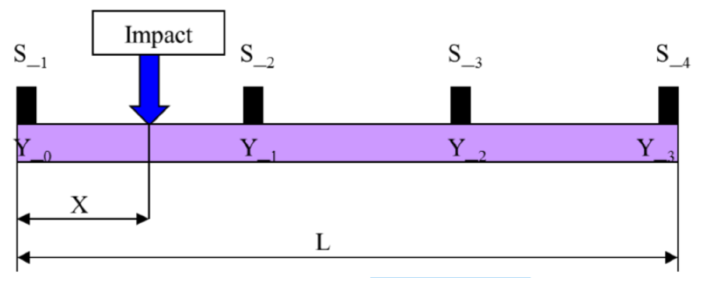
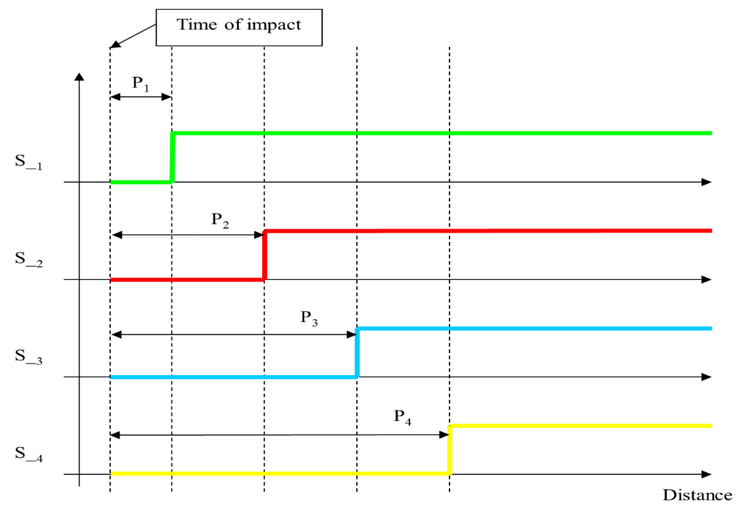
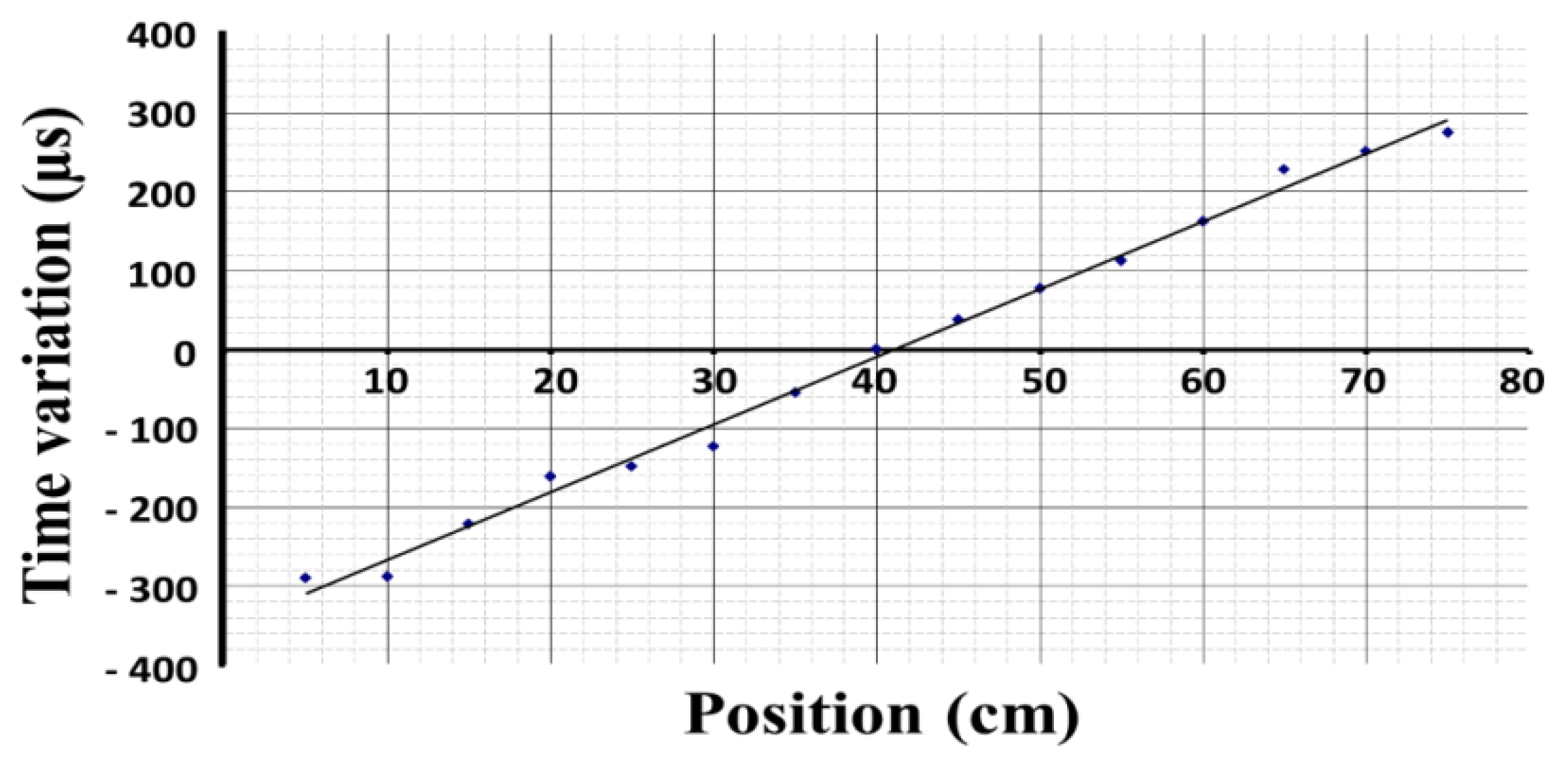
2.1. Location of an Impact on a Single Bar


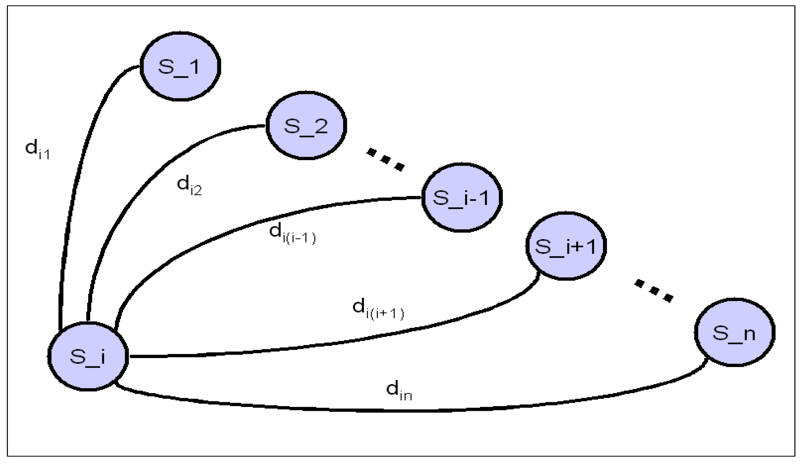
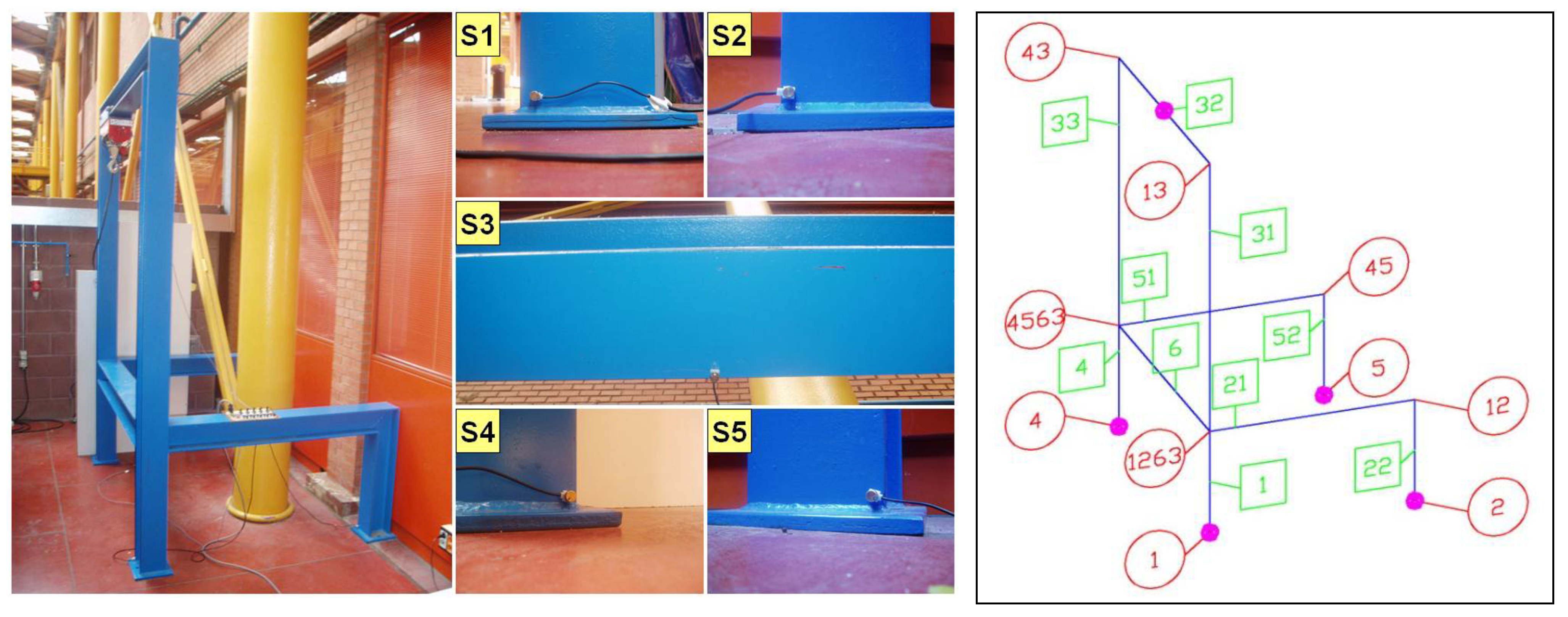
2.2. Locating an Impact on a 3D Structure

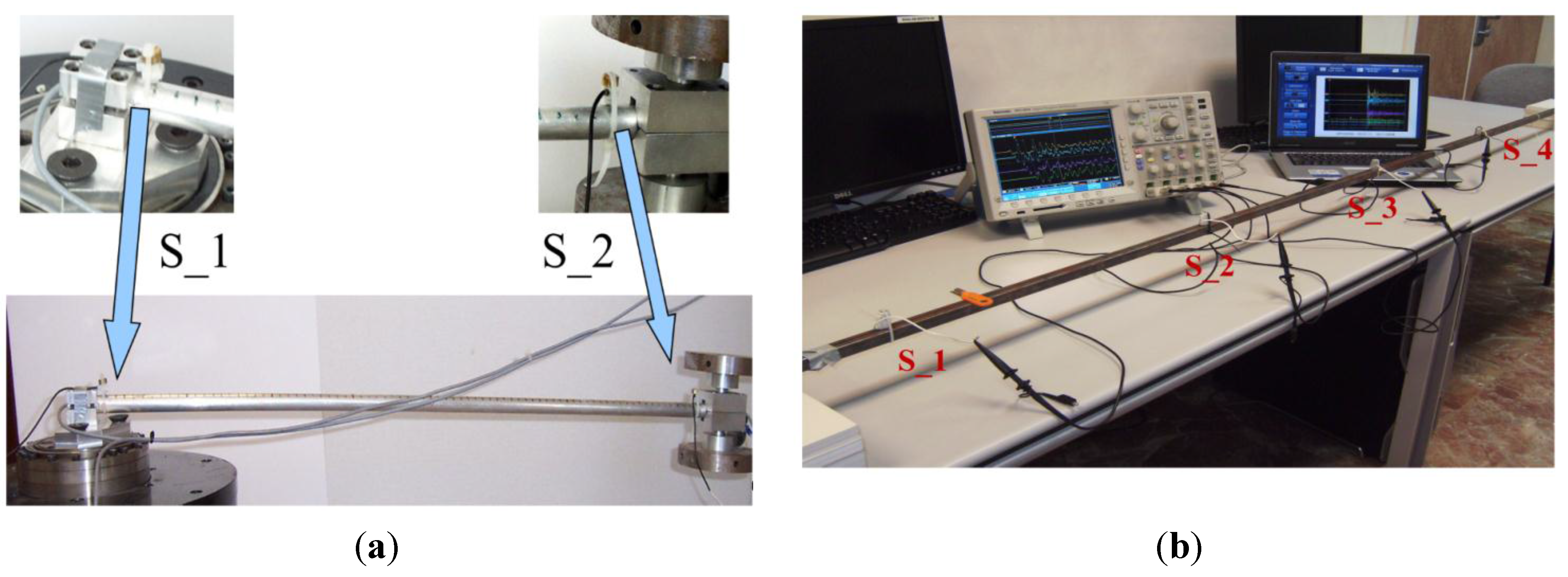
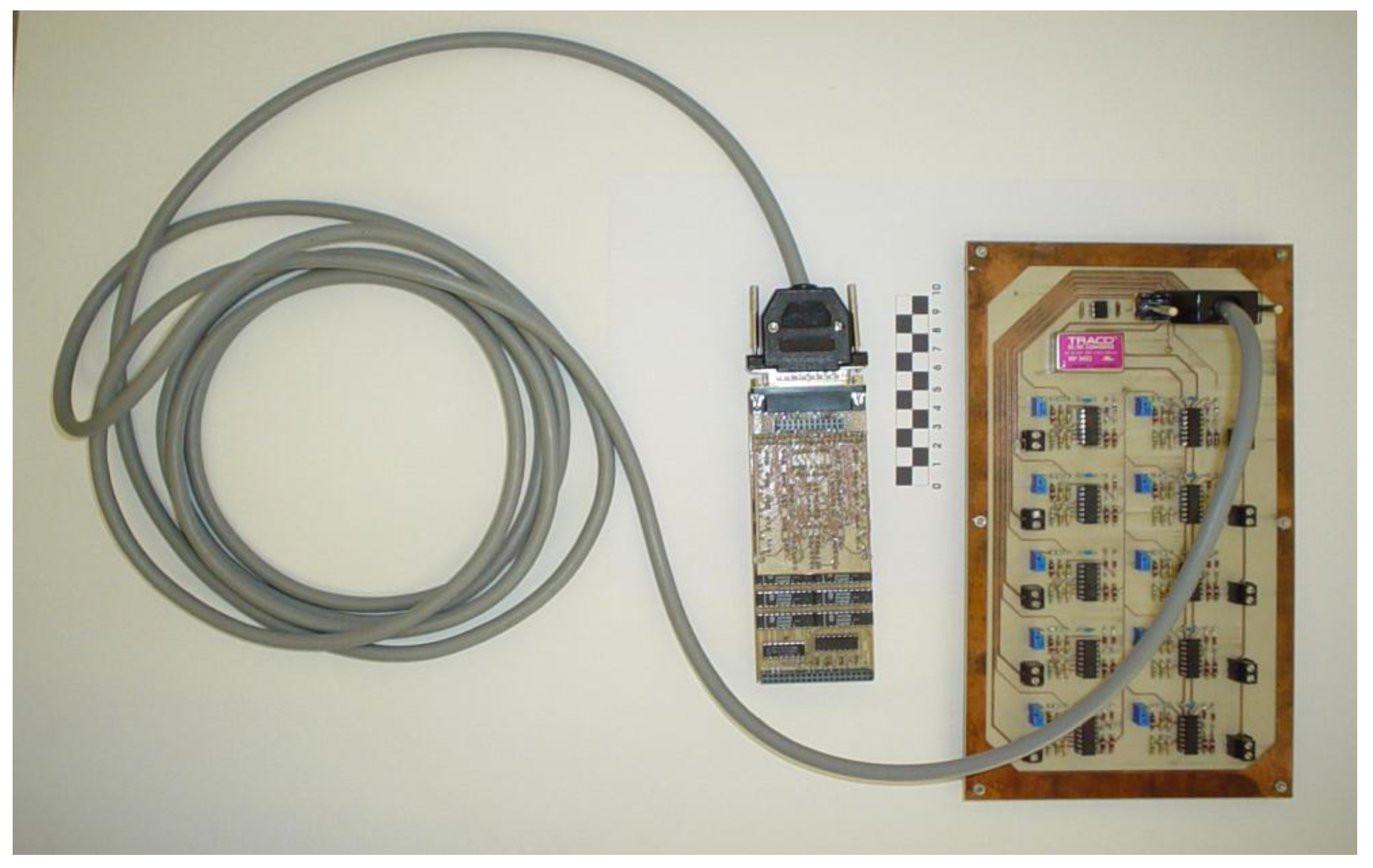
3. Experimental Setup


| Bar Number | From Node | To Node | Nominal Distance | Steel Profile |
|---|---|---|---|---|
| 1 | 1 | 1263 | 0.695 m | HEB 140 |
| 21 | 1263 | 12 | 1.360 m | HEB 130 |
| 22 | 12 | 2 | 0.695 m | HEB 130 |
| 31 | 1263 | 13 | 1.845 m | HEB 140 |
| 32 | 13 | 34 | 1.660 m | HEB 140 |
| 33 | 34 | 4563 | 1.845 m | HEB 140 |
| 4 | 4 | 4563 | 0.695 m | HEB 140 |
| 51 | 4563 | 45 | 1.360 m | HEB 130 |
| 52 | 45 | 5 | 0.695 m | HEB 130 |
| 6 | 1263 | 4563 | 1.660 m | HEB 160 |

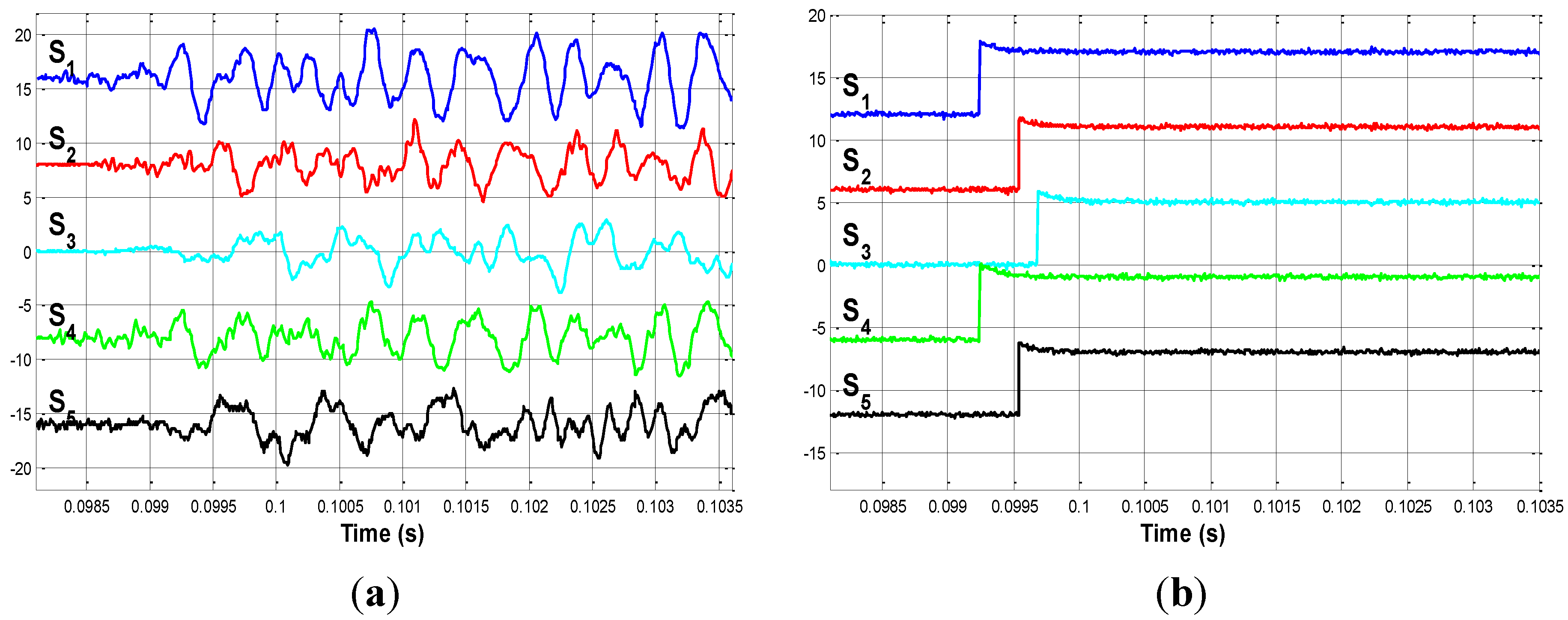
4. Results
4.1. First Impact: Impact on P_1

4.2. Second Impact: Impact on P_2

4.3. Third Impact: Impact on

4.4. Impact on

4.5. Impact on
4.6. Impact on
5. Conclusions
Acknowledgments
Author Contributions
Conflicts of Interest
References
- Briones, L.; Bustamante, P.; Serna, M. Robicen: A wall climbing pneumatic robot for inspection in nuclear power plants. Robot. Comput. Integr. Manuf. 1994, 11, 287–292. [Google Scholar] [CrossRef]
- Minor, M.; Dulimarta, H.; Dangi, G.; Tummala, L.; Mukherjee, R.; Aslam, D. Design and Implementation of a Miniature Under-Actuated Wall Climbing Robot. In Proceedings of the 2000 IEEE/RSJ International Symposium on Intelligent Robots and Systems (IROS), Takamatsu, Japan, 31 October–November 2000; Volume 3, pp. 1999–2005.
- Minor, M.; Mukherjee, R. Underactuated Kinematic Structures for Miniature Climbing Robots. ASME J. Mech. Des. 2003, 125, 281–291. [Google Scholar] [CrossRef]
- Balaguer, C.; Giménez, A.; Abderrahim, M. A Climbing Autonomous Robot for Inspection Applications in 3D Complex Environments. Robotica. 2000, 18, 287–297. [Google Scholar] [CrossRef]
- Giménez, A.; Balaguer, C.; Padrón, V.M.; Abderrahim, M. Design and path-planning for a climbing robot able to travel along 3D metallic structures. In Proceedings of the First International Symposium on Climbing and Walking Robots, CLAWAR’98, Brussels, Belgium, 26–28 November 1998.
- Balaguer, C.; Giménez, A.; Abderrahim, M. ROMA Robots for Inspection of Steel Based Infrastructures. Ind. Robot. 2002, 29, 246–251. [Google Scholar] [CrossRef]
- Mian, A.; Han, X.; Islam, S.; Newaz, G. Fatigue damage detection in Graphite/Epoxi composites using infrared imaging technique. Compos. Sci. Technol. 2004, 64, 657–666. [Google Scholar] [CrossRef]
- Drinkwater, B.W.; Wilcox, P.D. Ultrasonic arrays for nondestructive evaluation: A review. NDT&E Int. 2006, 39, 525–541. [Google Scholar]
- Honda, T. Non-destructive inspections for the aging degradation of machinery and structures. Reliab. Eng. Assoc. Jpn. 2007, 29, 350–357. [Google Scholar]
- Liu, Y.; Hu, N.; Xu, H.; Yuan, W.; Yan, C.; Li, Y.; Goda, R.; Alamusi; Qiu, J.; Ning, H.; Wu, L. Damage evaluation based on a wave energy flow map using multiple PZT sensors. Sensors 2014, 14, 1902–1917. [Google Scholar] [CrossRef] [PubMed]
- Liu, Y.; Goda, R.; Samata, K.; Kanda, A.; Ning, H.; Zang, J.; Ning, H.; Hu, N. An efficient algorithm embedded in an ultrasonic visualization technique for damage inspection using the AE sensor excitation method. Sensors 2014, 14, 20439–20450. [Google Scholar] [CrossRef] [PubMed]
- Shin, Y.W.; Kim, M.S.; Lee, S.K. Identification of acoustic wave propagation in a duct line and its application to detection of impact source location based on signal processing. J. Mech. Sci. Technol. 2010, 24, 2401–2411. [Google Scholar] [CrossRef]
- Hu, N.; Matsumoto, S.; Nishi, R.; Fukunaga, H. Identification of impact forces on composite structures using an inverse approach. Struct. Eng. Mech. 2007, 27, 409–424. [Google Scholar] [CrossRef]
- Atobe, S.; Sugimoto, S.; Hu, N.; Fukunaga, H. Impact damage monitoring of FRP pressure vessels based on impact force identification. Adv. Compos. Mater. 2014, 23, 491–505. [Google Scholar] [CrossRef]
- García, A.; Feliu, V.; Somolinos, J.A. Gauge Based Collision Detection Mechanism for a New Three-Degree-of-Freedom Flexible Robot. In Proceedings of the IEEE International Conference on Robotics and Automation, ICRA’01, Seoul, Korea, 21–26 May 2001; Volume 4, pp. 3853–3858.
- García, A.; Feliu, V.; Somolinos, J.A. Experimental Testing of a Gauge Based Collision Detection Mechanism for a New Three-Degree-of-Freedom Flexible Robot. Int. J. Robot. Syst. 2003, 20, 271–284. [Google Scholar] [CrossRef]
- Lewis, D.J. Airbag Module. US Patent Number US 6,425,601, 30 July 2002. [Google Scholar]
- Kazuto, M. Bend Detector for Impact rod. Japanese Patent Number JP20011349697, 21 December 2001. [Google Scholar]
- Kasten, A.; Franzen, J. Internal Detection of Ions in Quadrupole Ion Traps. GB Patent Number GB20010014075 20010608, 20 March 2002. [Google Scholar]
- Cortázar, O.D.; Feliu, V.; Somolinos, J.A. Detector Acústico de Impactos para Estructuras Mecánicas. SP Patent Number ES2273536, 7 June 2004. [Google Scholar]
- Somolinos, J.A.; Cortázar, O.D.; Feliu, V. Sistema de Detección y Localización de Impactos en una Barra Flexible. In Proceedings of the XXIV Jornadas de Automática, León, Spain, 10–12 September 2003. (In Spanish)
- Somolinos, J.A.; Morales, R.; García, A.; Morón, C. Piezoelectric Sensors System for Impact Detecting. Sens. Lett. 2013, 10, 1–3. [Google Scholar] [CrossRef]
- Somolinos, J.A.; López, A.; Morales, R.; Morón, C. A New Self-Calibrated Procedure for Impact Detection and Location on Flat Surfaces. Sensors 2013, 13, 7104–7120. [Google Scholar] [CrossRef] [PubMed]
- Dalton, R.P.; Cawley, N.; Lowe, M.J. Propagation of acoustic emission signals in metallic fuselage structure. IEE Proc. Publ. Sci. Meas. Technol. 2001, 148, 169–177. [Google Scholar] [CrossRef]
- Gómez, P. Estudio Comparativo de Procedimientos para la Detección y Localización de Impactos. Bachelor Thesis, E.U. Ingeniero Técnico Industrial, Universidad Carlos III de Madrid, Leganés, Spain, 2008. [Google Scholar]
- León, C. Sistema Electrónico para Detección y Localización de Impactos. Master’s Thesis, Ingeniero Industrial, Universidad de Castilla-La Mancha, Ciudad Real, Spain, 2003. [Google Scholar]
- Atobe, S.; Kobayashi, H.; Hu, N.; Fukunaga, H. Real-time impact force identification of CFRP laminated plates using sound waves. In Proceedings of the 18th International Conference on Composite Materials, Jeju Island, Korea, 21–26 August 2011; pp. 1–6.
© 2015 by the authors; licensee MDPI, Basel, Switzerland. This article is an open access article distributed under the terms and conditions of the Creative Commons Attribution license (http://creativecommons.org/licenses/by/4.0/).
Share and Cite
Morón, C.; Portilla, M.P.; Somolinos, J.A.; Morales, R. Low-Cost Impact Detection and Location for Automated Inspections of 3D Metallic Based Structures. Sensors 2015, 15, 12651-12667. https://doi.org/10.3390/s150612651
Morón C, Portilla MP, Somolinos JA, Morales R. Low-Cost Impact Detection and Location for Automated Inspections of 3D Metallic Based Structures. Sensors. 2015; 15(6):12651-12667. https://doi.org/10.3390/s150612651
Chicago/Turabian StyleMorón, Carlos, Marina P. Portilla, José A. Somolinos, and Rafael Morales. 2015. "Low-Cost Impact Detection and Location for Automated Inspections of 3D Metallic Based Structures" Sensors 15, no. 6: 12651-12667. https://doi.org/10.3390/s150612651