Article

Characterizing the Heterogeneity of the OpenStreetMap Data and Community

Faculty of Engineering and Sustainable Development, University of Gävle, SE-801 76 Gävle, Sweden
*
Author to whom correspondence should be addressed.
ISPRS Int. J. Geo-Inf. 2015, 4(2), 535-550; https://doi.org/10.3390/ijgi4020535
Submission received: 6 January 2015 / Revised: 9 March 2015 / Accepted: 27 March 2015 / Published: 8 April 2015

Abstract

:
OpenStreetMap (OSM) constitutes an unprecedented, free, geographical information source contributed by millions of individuals, resulting in a database of great volume and heterogeneity. In this study, we characterize the heterogeneity of the entire OSM database and historical archive in the context of big data. We consider all users, geographic elements and user contributions from an eight-year data archive, at a size of 692 GB. We rely on some nonlinear methods such as power law statistics and head/tail breaks to uncover and illustrate the underlying scaling properties. All three aspects (users, elements, and contributions) demonstrate striking power laws or heavy-tailed distributions. The heavy-tailed distributions imply that there are far more small elements than large ones, far more inactive users than active ones, and far more lightly edited elements than heavy-edited ones. Furthermore, about 500 users in the core group of the OSM are highly networked in terms of collaboration.

1. Introduction

Twenty-first century society benefits considerably from, and is increasingly driven by, two forces characterized by the head and the tail of a long-tail distribution [1]. For example, while the telephone industry was dominated by national telecoms such as AT&T, we now have services such as Skype. The Encyclopedia Britannica was very popular, but we now have a free and more popular counterpart in Wikipedia. Information was controlled by governments and giant mass media such as CNN, but WikiLeaks or OpenLeaks recently made history by freely sharing information. In the same vein, volunteered geographic informaton (VGI) [2] emerged as a counterpart to geographic information, which is conventionally collected and maintained by national mapping agencies. As part of user-generated content in the era of Web 2.0, VGI uniquely provides geo-referenced location information. OpenStreetMap is the most successful and well-known project of VGI, which has attractedd significant and sustained interest in academy, industry, and governmental agencies.
In this article, we study all OSM data collected over the past decade, submitted by about 1 million registered users up to February 2013. Previous studies showed that both the data and the user community are very heterogeneous. For example, only a small percentage of users make almost all the contributions, including creation and edits [3,4,5]. In terms of data concentration and accuracy, the OSM data varies dramatically from urban to rural areas, or from country to country [6,7]. However, these previous studies were conducted mostly at country and city levels. They lack quantitative indicators about heterogeneity or variation. In contrast, we examined all the OSM data and its history to present a holistic picture of OSM based on power-law statistics and the head/tail breaks-induced ht-index. More specifically, we illustrate and quantify the underlying heterogeneity of the OSM elements, the users, and their contributions through a set of quantitative metrics such as α, p value and ht-index.
Power-law statistics is based on the robust maximum-likelihood estimation, which differs from the conventional least-square estimation [8] (see Section 3 for more details). The maximum-likelihood estimation provides two metrics: α (degree of heterogeneity), and p value (goodness of fit). On the other hand, the head/tail breaks [9] is a newly developed classification scheme for data with a heavy-tailed distribution. It is also an efficient, effective visualization tool for big data [10]. Head/tail breaks partitions the whole around an average size into many small things in the tail being a majority, and a few large ones in the head being a minority. This partition continues recursively for the head (the large things) until the notion of far more small things than large ones is violated. Eventually, the number of times that far smaller things recur is defined as the ht-index [11] for characterizing complexity or hierarchical levels of the whole.
The contribution of this paper is three-fold. We situated the study in the context of big data and extracted the related historical and attribute information from the entire OSM databases and the users’ historic archive. Based on the extraction, we characterized the heterogeneity of OSM databases and discovered very striking scaling patterns for both users and data. We built up the co-contribution networks over the eight-year timespan of data and found the underlying nonlinear characteristics of OSM user collaboration networks.
The remainder of the paper is organized as follows. Section 2 presents the OSM history data and the working procedure of processing the huge dataset. Section 3 briefly introduces the methodology for conducting the scaling analysis, including power law statistics and detection and the head/tail breaks. Section 4 shows the statistical results of the scaling patterns and other results. Section 5 further discusses the implications of this study. Finally, Section 6 draws conclusions, and points to future work.

2. Data and Data Processing

Started in July 2004, and motivated by the great success of Wikipedia, OSM aimed to provide free editable maps for the entire world [12]. A large number of volunteers relied on GPS receivers to collect GPS trajectory data and transformed it into map data using online editing tools. The mapping processes are time-consuming and tedious. In 2006, Yahoo! donated digital images freely to the OSM community, so that mapping could be done directly from the images. Later on, OSM obtained free data sets freely from companies and countries, such as a complete road data set of Netherlands donated by Automotive Navigation Data, and the transformation of a US Census TIGER road data set. Over the past decade, OSM has become one of the largest geodata sources and most famous VGI platform with around 1.8 million users and billions of geographic elements.
The OSM data is freely accessed on the Internet and with a number of supported formats such as XML and shape files. This study uses the complete OSM data history dump, which can be downloaded via [13]. The dump is huge, at 692 GB collected from 9 April 2005 to 5 February 2013 in XML format. It mainly includes and is structured sequentially by three basic types of geographical elements of OSM data: node, way and relation. Nodes as point features that store the location information of longitude and latitude coordinates. Ways are polylines and polygons that contain a set of ordered nodes. Relations denote the geographic relationships among the three types of elements. Each element contains a variety of information such as id, timestamp of creation or edits, contribution user and user id, version number, and different kinds of tags. The historical information is organized by version numbers with the attribute name version, which increases by 1 each time there is a new version of this element.
It is difficult to work with on such a big file, since simply running it through takes several hours on a state-of-the-art desktop computer. We therefore developed a working procedure (Figure 1) to extract both historical and attribute information for each element of the entire database for further analysis. For the historical information, we collected element ID, timestamp, contributing user ID and version number at each version. Attribute information of each element was with respect to the latest version. For each node element, we extracted its coordinate pair (latitude and longitude), and for each way and relation element, we collected their member IDs. The whole process took three days on an eight-core 3.4GHz CPU and 32GB memory desktop. The extraction was organized as a big table and formatted as a txt file with a size of about 150 GB, including approximate 2.1 billion elements consisting of 1.9 billion nodes, 0.2 billion ways and 2 million relations. For further analysis, we calculated the number of users, edits, and sizes for each element and their spatial distribution at the country level (see detailed description in Section 4). The extraction as a shrunk version of data greatly improves efficiency, as it only takes half an hour to traverse the file and less than one second to return query results by using a binary search based on sorted element ID.
Figure 1. Flow chart for the data processing to extract essential information for further analysis. Note that (a) is data processing and (b) is results
Ijgi 04 00535 g001

3. Methodology

This study illustrates a set of adopted nonlinear methods, including power-law detection based on maximum-likelihood estimation [8] and the head/tail breaks as a classification scheme for data with a heavy-tailed distribution [9]. We rely on these two methods for scaling analysis because (1) the power law detection is probably the most robust and reliable method for power law estimation; and (2) the head/tail breaks can act as both a classification scheme and visualization tool [10]. These two methods greatly complement each other to uncover and visualize the underlying scaling properties of OSM data. More specifically, power-law detection is concerned with how a data set fits better than any other alternatives such as lognormal, exponents and their variants, while the head/tail breaks aims to reveal the inherent hierarchical levels or the head/tail breaks induced ht-index [11]. More importantly, the head/tail breaks can efficiently and effectively filter out redundant data as a powerful visualization tool for big data.

3.1. Power Law Detection

Data bearing the scaling property follows a power law distribution, which means that the frequency of each value is inversely proportional to the power of its rank. In other words, the data contains far more small values yet very few large values. The most famous example of power law is found in word occurrences, city sizes, and wealth distributions [14]. Generally, the power law is denoted as:
y=k x α
in which k is a constant, and α is the power law exponent.
The simplest way to detect the power law is to take logarithm scale on both axes to see if the distribution curve is a straight line, based on:
ln( y )= αln( x )+ln( k )
However, this method suffers from the messy tail at the very end of the distribution. Hence, Clauset et al. [8] have introduced a rigorous statistical test based on maximum likelihood and the Kolmogorov-Smirnov (KS) test for power law detection. There are two parameters: an estimated exponent α and the index of a goodness-of-fit p. They are used as indices for power-law fit and the goodness of the fit. This method has been widely used and proved to be robust for detecting the power-law distributions with a wide range of complex systems [15,16,17].
Simply put, the estimated exponent α is used to shape the power-law distribution and the acceptance range is from 1 to 3, given by:
α=1+n [ i=0 n ln x 1 x min ] 1
in which α denotes the estimated exponent, and xmin is the smallest value above which the power law fit is held.
We adopted a modified KS test to assess how data fits a power-law distribution (goodness-of-fit). It is based on the idea that the maximum distance (D) between the cumulative density functions (CDF) of the data and the fitted model:
D= | f( x )g( x ) | x x min max
in which f(x) is the CDF of the data for the observations with a value at least xmin, and g(x) is the CDF for the power-law model that best fits the data where x x min .
Usually, 1000 synthetic data sets are then generated with the fitted model g(x), which contain data whose values above xmin perfectly follow a power law distribution. Conversely, values below xmin are not power-law distributed. The maximum difference D is re-calculated between the fitted model and each synthetic dataset. The goodness-of-fit index p is denoted as a fraction of the number of Di whose values greater than D to 1000. The higher the p value, the better fit the power law. The closer the p-value reaches to 1, the more the data is accepted for a power law distribution. The acceptable threshold as a goodness of fit is considered to be 0.05.
Power-law detection is probably the toughest statistical estimation to differentiate power laws from other alternatives such as lognormal, exponential and other variants. In contrast to the rigorous power law detection, the head/tail breaks provides a simple solution to reveal the underlying scaling, and it applies all kinds of heavy-tailed distributions, as long as the scaling pattern of far more small things than large one recurs multiple times.

3.2. Head/Tail Breaks

The head/tail breaks is basically originated from the main characteristic of heavy-tailed distributions. Given data with a heavy-tailed distribution, the arithmetic mean, or average, can split all the data values into two unbalanced parts: A minority of big values above the mean, called the head; and a majority of small values below the mean, called the tail. This process recursively continues for the head until the notion of far more small values than large ones is violated; see the following recursive function namely head/tail breaks. The percentage of splitting up data into the head and tail is set at 40 percent. This implies that the tail percentage is 60 percent. The number of times the data can be split plus 1 is the ht-index [11]. It captures how many times the scaling pattern of far more small things than large ones recurs in the data. It quantifies the scaling characteristic of the data. The higher the ht-index, the more hierarchical levels in the data.
Recursive function Head/tail Breaks:
     Break the input data (around mean or average) into the head and the tail;
    // the head for data values above the mean
    // the tail for data values below the mean
     While (head <= 40%):
        Head/tail Breaks(head);
End Function
		
Some data in this study, such as 2 billion elements, were too big to detect the power laws. In this regard, head/tail breaks provide a nice solution. Instead of taking all the elements, we took the head part for power-law detection. If the head part was still too big, we took the next head part, until the head part was small enough for power-law detection. The reason why we recursively take the head is simply because the head is self-similar to the whole data set. This is also the fundamental argument for the head/tail breaks as an efficient, effective visualization tool for big data [10]. Therefore, power-law detection and head/tail breaks complement each other and provide powerful tools for revealing the underlying scaling or heterogeneity of the OSM data.

4. Scaling Properties of the OSM Data

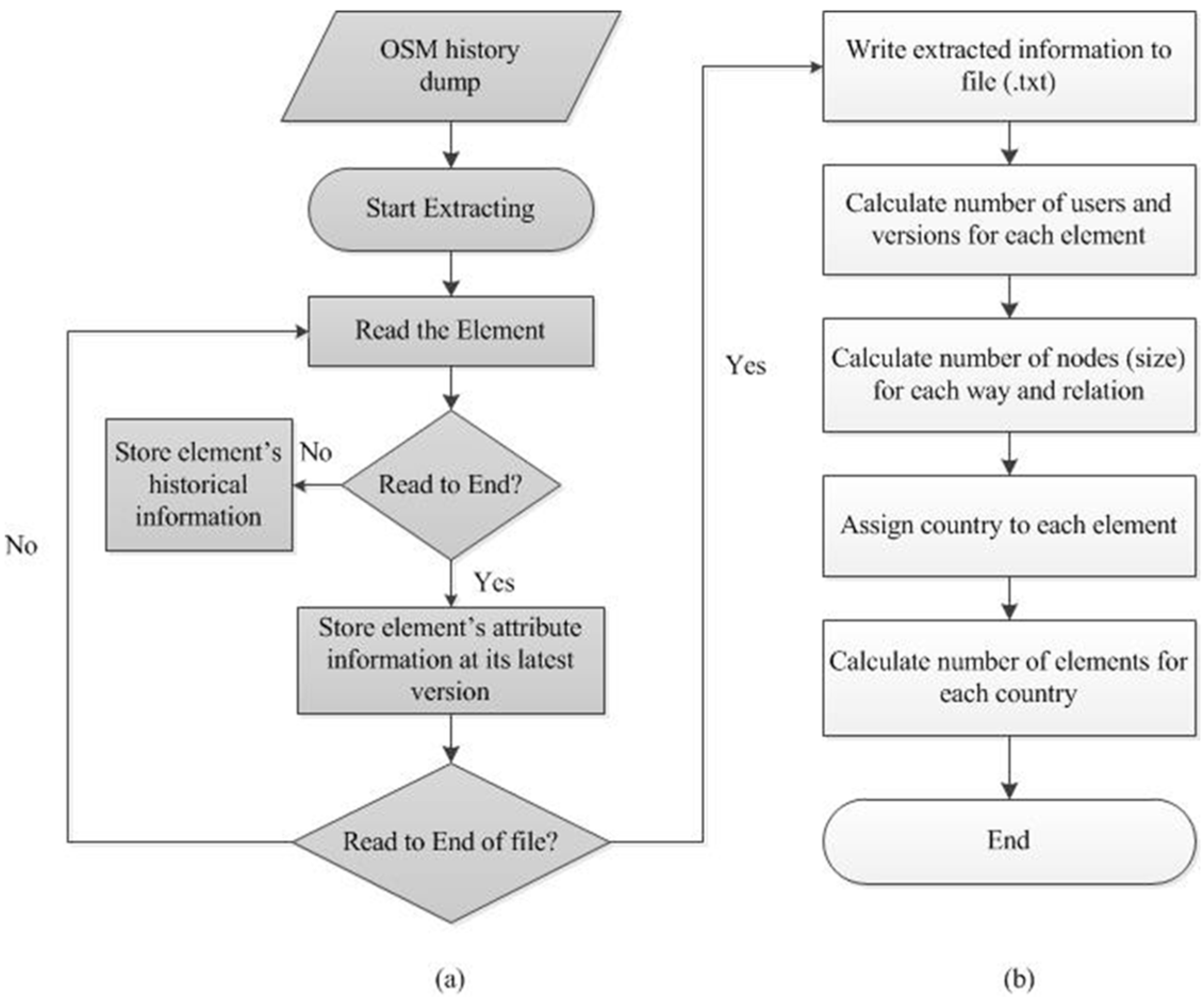
This section presents the results of the scaling analysis on a variety of features based on three aspects in the context of big data including 1 million users, 2.1 billion elements and 2.7 billion contributions (Figure 2). These three parts constitute an interconnected picture of the OSM data and community. The users contribute to the elements, leading to a great increase in both element volume and complexity, and the user community. Through the contributions, users formed an interconnected collaboration network. The scaling analysis based on power-law detection and head/tail breaks was applied to these three aspects to examine to what extent the scaling pattern of far more small things than large ones was true for the OSM data.
Figure 2. Three aspects of the study in the context of big data.
Ijgi 04 00535 g002

4.1. On Users and Elements

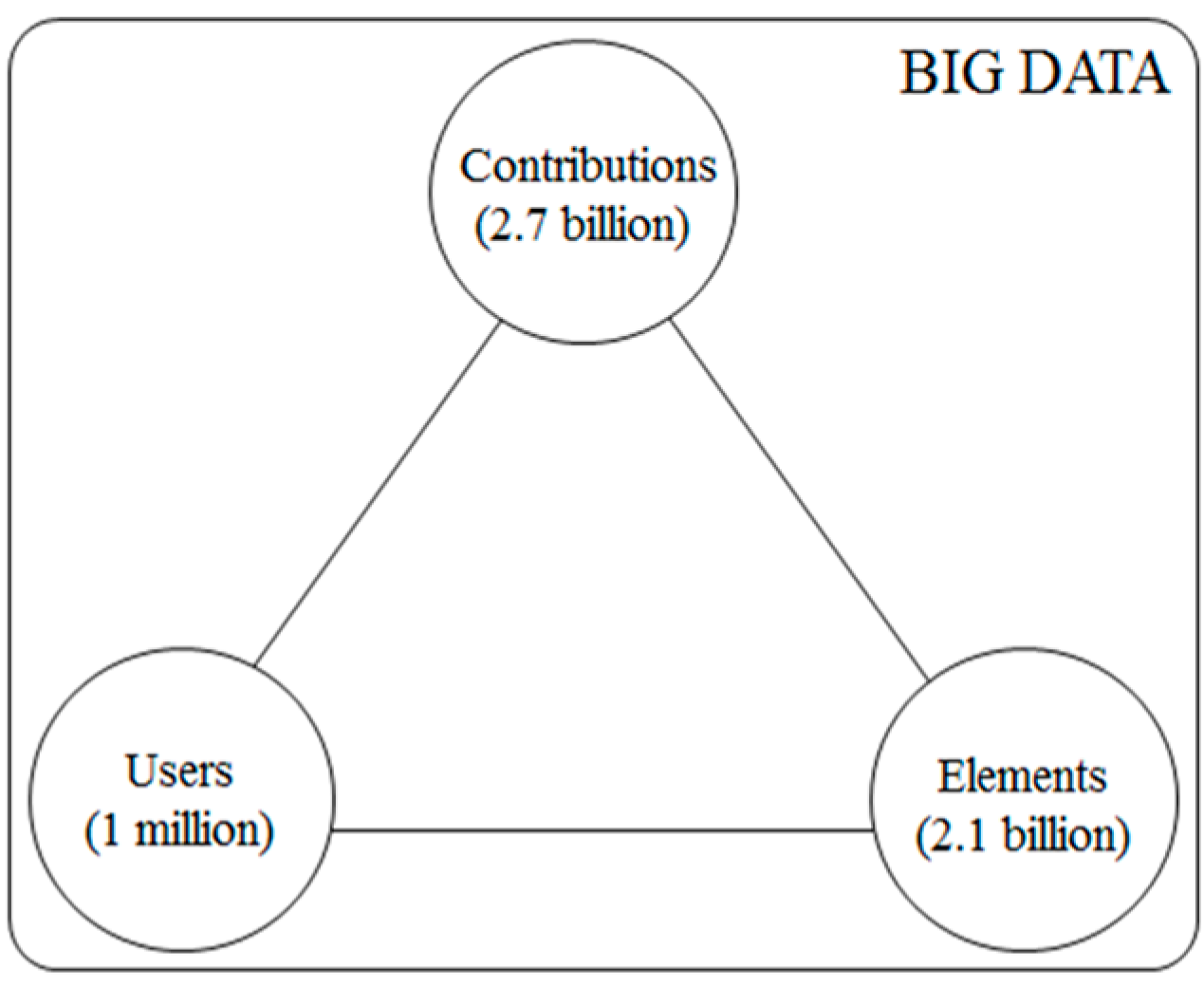
We first investigated users based on their number of contributions. The investigation was based on how many unique element IDs can one user contribute to. These contributions include both creating and editing. A total of 268,227 users made contributions. The number of each user’s contributions exhibited a power-law distribution, with an accepted α of 2.24 and p value of 0.26 (Figure 3a). By applying the head/tail breaks, we derive the scaling hierarchy of these numbers, indicated by the ht-index of 7 and very low percentages for each head (<30%). This means the strikingly scaling pattern recurs 6 times of this data (Table 1). This apparent scaling pattern indicates that only a very small number of users contributed the majority of OSM elements. In other words, there are far more inactive users than active ones.
Table 1. Head/tail breaks statistics for user contributions (Note: # = number, % = percentage).
# Sum# Head% Head# Tail% TailMean
268,22713,2414%254,98696%10,232
13,241182513%11,41687%199,020
182530716%151884%1,164,797
3074815%25985%4,751,085
48816%4084%18,843,785
8225%675%69,899,060
Secondly, we looked at different attributes of elements. Each element is characterized by the number of users, edits and size respectively. Specifically, the number of users for each element indicates that how many users contribute to it, given by the number of unique user ids of this element. Note that the contribution includes both creation and edit; the number of edits can be directly obtained by the maximum version number of this element, since it equals to maximum version number minus one. The number of size refers to how many unique node ids it contains. The size of each node element is always 1; the size of each way element equals to the number of its unique comprising points; the size of each relation element is determined by the number of unique points its member contains: node, way or relation (these three members do not always exist simultaneously in one relation). Because some relation elements can have other relation element(s) as its member(s), it is difficult to calculate those relation elements’ sizes when they mutually contain each other as their member(s). There were 4356 relation elements excluded because of such complicated structures. Considering the elements of 2.1 billion studied, we believe that the 4356 excluded would not affect much on our results.
Next, we applied head/tail breaks to the above three aspects. All three derived ht-indices were very high (>10), and most of the head percentages were small (<30 percent; see detailed results in the Appendix). It indicates that there are far more small elements than large ones. Power-law detection was further applied on the data of the top hierarchical levels of each category (Table 2). The “filtered” data was the proxy of the whole since the scaling pattern remains at each level. Only the number of element size passed the power law test (Figure 3d). The number of element users and edits can still be considered as heavy-tailed distributed as observed from the Figure 3b and 3c that each plot is close to a straight line at logarithm scales, therefore we think that the entire dataset of three aspects possess a strong scaling property. We also examined the evolution of data on a yearly basis and found that heterogeneity was no different from the data as a whole. In other words, the data for the previous years are all heavy-tail distributed, but vary with different ht-indices.
Table 2. Summarized statistics on OpenStreetMap (OSM) elements on top hierarchies in three categories.
# ElementsMaxMinαp
User745,94319774.950
Edit548,9143084313.390.006
Size479,0045,118,2765642.370.13
Figure 3. Power-law distributions of user contributions: (a) number of users; (b) number of edits; and (c) number of sizes (d) of each element. The data for (b), (c), and (d) are selected from the top hierarchies of all elements. (b) and (c) are not power-law distributed because both α values are larger than 3, but they are heavy-tailed, illustrated by the high ht-index shown in the Appendix.
Ijgi 04 00535 g003
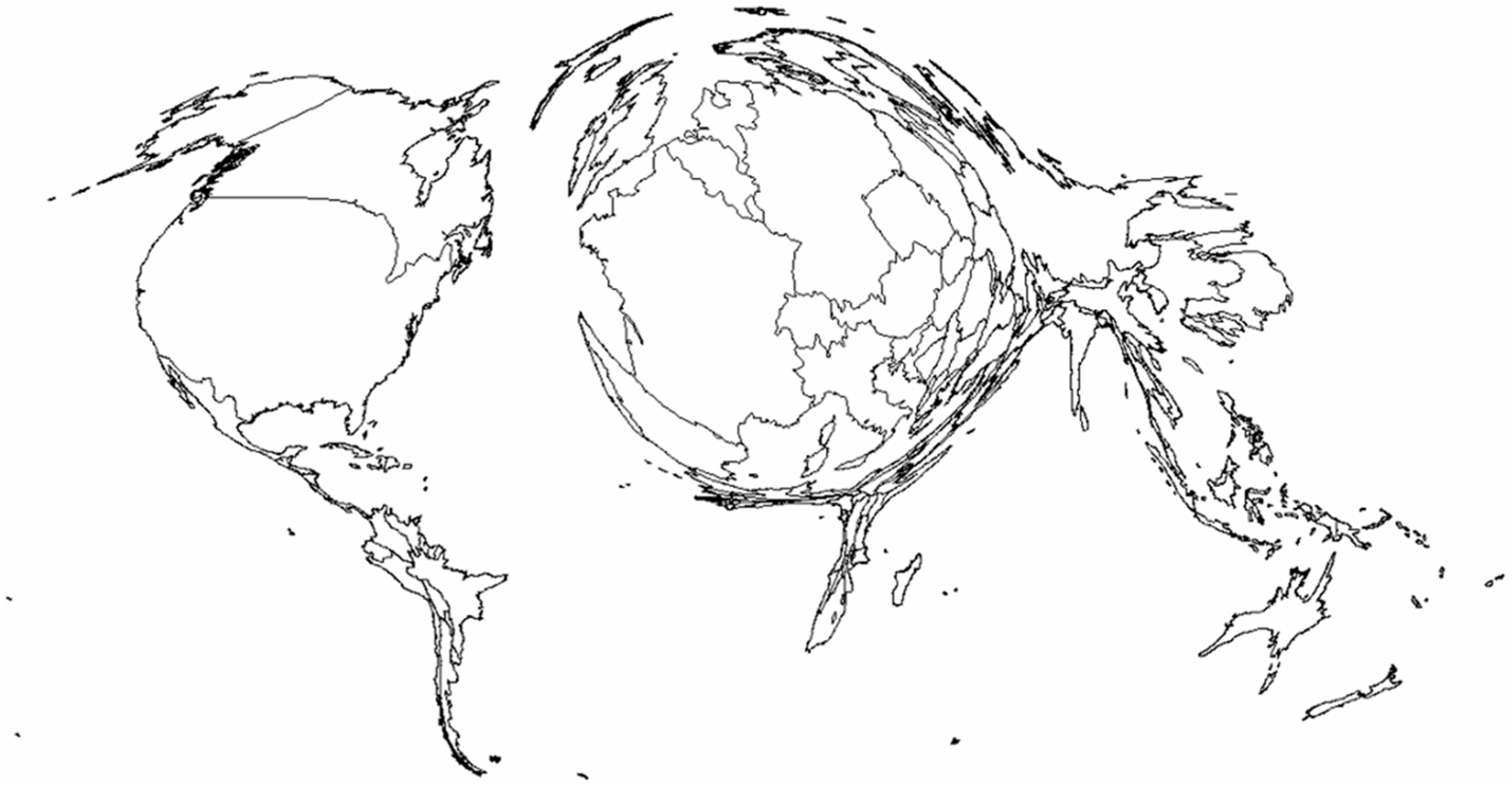
We further inspected the spatial distribution of the elements, i.e., how many the elements are located in each country. We computed and assigned to each country the number of elements and the aggregated attribute values of each aspect. As results, the data of all the three aspects are very power-law distributed (Table 3), which indicate that there are far more small countries than large ones all over the world in terms of the elements, users and contributions and it further implies that the high variation of quality and completeness of OSM database from country to country through different elements concentrations. The cartogram shows the resulting country sizes (Figure 4), of which the top 5 countries are US, France, Canada, Germany and Russia. These countries are also the top 5 ones in terms of aggregated numbers of users, edits and size, but with a slightly different ranking (Canada and Germany switch positions).
Table 3. Summarized statistics of elements at country level.
maxminαp
#Element401,137,3048361.740.87
#User598,175,4419511.740.82
#Edit636,597,3639691.730.71
#Size898,145,60014081.690.67
Figure 4. The cartogram showing the spatial distribution of global OSM elements at country level.
Ijgi 04 00535 g004

4.2. On Co-Contribution Network

Having examined the users and elements, we subsequently studied the scaling pattern in the collaboration network of the OSM users. The social relationship utilized in this research is co-contribution relationship since friend relationship like other social platforms (e.g., Facebook) is undocumented in OSM history. The collaboration or co-contribution relationship is established in the OSM data archive when more than one user contributes to the same element. In other words, we considered that user has such relationship with others if they either create or edit the same element. This approach is different from the one defined by Mooney and Corcoran [4,
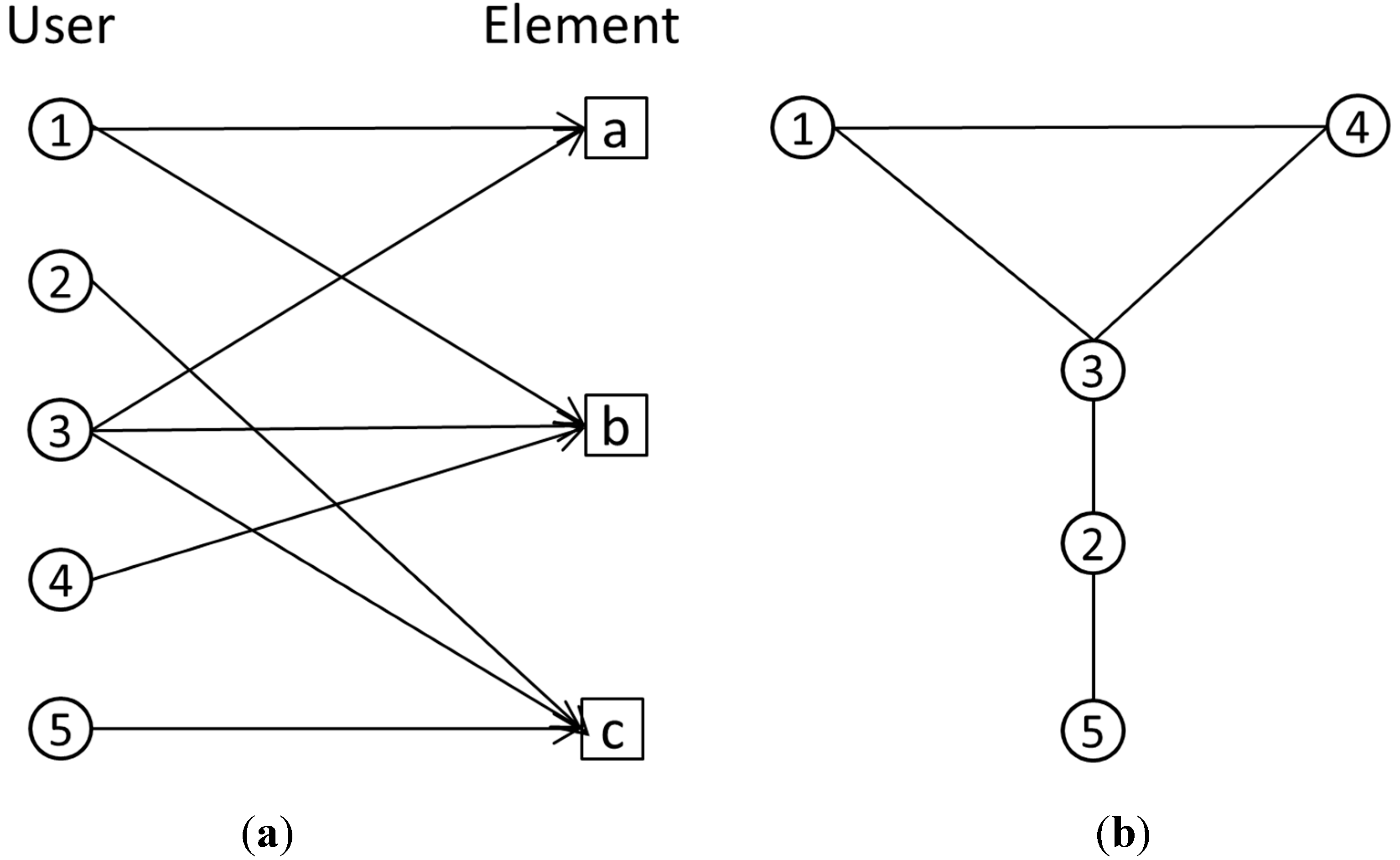
18] who consider only the edit interaction and also the sequence of edits. In this regard, we construct a “co-contribution network” rather than co-edit network. As Figure 5a shows, assuming that user 1, 3 and 4 make contributions to element b, there are co-contribution relationships between every two of them, so that the resulting network (Figure 5b) can be obtained. Note that this paper considers only the binary network, which consists of undirected and unweighted edges.
Figure 5. Illustration of co-contribution relationship. Users’ contributions to elements are represented as a bi-partite graph (a), which is transformed into a co-contribution network (b).
Ijgi 04 00535 g005
Following the rule of co-contribution relationship, we built up the network based on the entire history of all the elements to better illustrate engagement in the OSM community [19]. The resulting social graph consists of 248,070 nodes and 6,446,086 edges. The node degree of this network is power-law distributed and has an ht-index of 10 (Table 4), indicating that the network is extremely scale-free. 
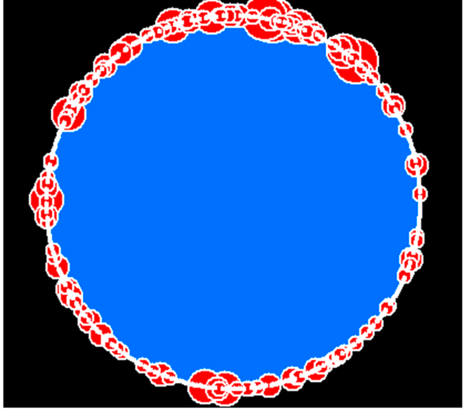
Figure 6 shows the “filtered” network comprising 477 nodes of the top 5 hierarchies as the representative of the entire network, from which the underlying scaling pattern is clearly uncovered. We further examine the networks of previous years from 2005 in order to see if scaling pattern persists all the time during the evolution of the OSM community in terms of contributions. As results, except that no existence of such network between the years of 2005 and 2006, the evolution of co-contribution networks is with a nonlinear growth of both nodes and edges from 2007 onwards and becomes increasingly scaling which is indicated by the power-law fitting metrics and overall increasingly large ht-index of each year (Table 5).
Table 4. Head/tail breaks statistics for node degree of co-contribution network in 2013.
# nodes# head% head# tail% tailmean
248,07033,50413%214,56687%51.97
33,504726721%26,23779%322.08
7267182025%544775%1037.53
182047726%134374%2486.16
47713728%34072%5181.7
1374029%9771%9474.48
401127%2973%16,102.82
11327%873%26,460.73
3133%267%47,980.33
Figure 6. The co-contribution network for the top five hierarchical levels involving 477 nodes and 80,957 edges. The scaling hierarchy of far more small nodes than larger ones is indicated by the size of red dots.
Ijgi 04 00535 g006
Table 5. Scaling analysis results of co-contribution networks from 2007 to 2013.
2007200820092010201120122013
# of nodes385625,13360,231101,364159,747240,119248,070
# of edges29,701418,0771,306,1542,415,3193,954,8266,192,5106,446,086
max-degree802544915,05230,81651,50165,19065,876
ht-index879991010
α2.82.682.572.592.642.532.91
p0.460.650.180.140.0600.2
We also developed some insights into OSM community in term of user collaboration from the derived co-contribution network. Comparing to the collaboration network of English Wikipedia [20,21,22], it has the same scaling pattern of far more inactive users than active ones. In addition, the network also has some high density concentrations, especially among those highly active users. Specifically, each user averagely collaborates with around other 52 users in the whole network and those high degree users even have collaboration with almost every other. We further select two global location-based social networks (Gowalla and Brightkite) for comparison (data are available at [23]) and find that the co-contribution network is much denser than them regarding to both the whole and sampled (nodes of top hierarchies) network.

5. Further Discussions on the Study

From the results presented in Section 4, we can remark a great heterogeneity of the OSM data and community from the elements to user contributions, and further to the annual co-contributions networks. All of them can be well characterized by the striking scaling patterns, which are indicated by some metrics of power-law statistics and underlying hierarchies and additional statistics of head/tail breaks. This section further discusses some implications of the results and the study in general.
In this study, we have processed and analyzed the entire OSM data and community archive from a holistic perspective involving elements, users and their collaboration networks evolving over the past decade. Over hundreds of gigabytes of the data are processed and computed to develop new insights into the data and community. The findings of this study are in line with previous research on users and elements [3,4,5,24] that a minority of users/elements accounts for a majority of contributions/edits. The major difference between our work and the previous studies is that we conducted an in-depth quantitative analysis on all users and elements at the global scale. This enables us to see something that has not been illustrated in the previous works. To our best knowledge, the scaling patterns have never been examined for OSM dataset at such a massive level. In this connection, we believe that this study can be extended to other user-generated content such as Wikipedia [21].
This paper applies the scaling analysis to characterize the heterogeneity of global OSM database. Apart from examining the power law statistics for detecting scaling patterns, other heavy tailed distributions are observed and measured by the ht-index. It is widely known that the data formed from real-world phenomena are very likely to be heavy-tailed distributed as the case with the OSM data, since the data are naturally evolved and accumulated from individuals from the bottom up instead of imposed by authorities from the top down. As results, the data of all aspects follow power laws or heavy tailed distributions in general. Therefore, conventional linear methods like Gaussian statistics show some inadequacies in characterizing this kind of heterogeneity. Simply there is no typical mean or scale to characterize the heterogeneity; instead the scaling across all the scales can be used to characterize the diversity or heterogeneity. Our study points to the argument that in the big data era geospatial analysis requires a new way of thinking—The Paretian thinking [25] for better understanding geographic forms and processes.
Big data, due to its diversity and heterogeneity, is likely to demonstrate the scaling pattern of far more small things than large ones. The large and small things constitute the head and tail, respectively, of a long-tail distribution. Interestingly, the scaling pattern recurs multiple times, which implies that the things in the head demonstrate the scaling pattern of far more small things than large ones, again and again. This recurring scaling pattern is what underlies the new classification scheme called head/tail breaks [9]. The head/tail breaks divides things around an average into a few large things in the head and many small things in the tail, and continue recursively for the dividing process for the head until the notion of far more small things than large ones is violated. The head/tail breaks can efficiently and effectively filter out data while data is too big to handle. This filtering function is also what underlies the visualization function of head/tail breaks [10]. We believe that the head/tail thinking behind the head/tail breaks is very promising for big data and its analytics.

6. Conclusions

OSM data are essentially very heterogeneous either at a local or the global scale. This is because geographic space or the earth’s surface is very heterogeneous—no average location on the earth surface. In this paper, we study the entire OSM data and find that this heterogeneity can be fairly illustrated and measured from the element, users, and their collaborations. For the users, both their contributions and the degree of the co-contribution networks exhibit a clear power law distribution, which means that there are far more inactive users than active users; for elements, there are far more small elements than large ones since their attribute values throughout three categories (number of users, edits and size) are heavy tail distributed. In addition, the elements assigned to individual countries demonstrate a striking power law. Moreover, such pattern also remains at the country level concerning the spatial distribution of all elements. The head/tail breaks can be utilized as an efficient and effective tool to analyze and visualize the big data in capturing the underlying scaling hierarchies and complement the mathematical power law detection. To summarize, the scaling property is clearly shown with the OSM data and can well-characterize this great heterogeneity through power law fitting metrics and underlying the scaling hierarchical levels.
The study is conducted from the big data perspective, which focuses on the entire dataset and data-intensive computing [26]. Therefore, we have created a comprehensive image of the heterogeneity of the OSM data and obtained a valuable dataset with respect to the historical and attribute information of all elements at the certain time point. Interested researchers are always welcome to contact us for further detailed information on the data processing. As for the future work, two things should be done. The first is to take the tag information of each element into account and conducting the scaling analysis on them. The second is to study the nonlinear dynamics of both spatial and attribute information of each element at different temporal granularities (e.g., year, month, week etc.) to find the underlying mechanism of the evolution of both OSM community and user mapping activities.

Author Contributions

Ding Ma, Mats Sandberg and Bin Jiang designed the study and wrote the paper together. Ding Ma did the programming on data processing and computed the metrics. Bin Jiang and Mats Sandberg were in charge of revising the manuscript.

Appendix: The Head/Tail Breaks Statistics for Users, Edits, Sizes

To supplement the description of the results presented in Section 4.1, this appendix contains the detailed statistics on the head/tail breaks process for the three aspects: users, edits, and sizes. As we can see, all the data have more than 12 hierarchical levels, shown in the level column, and the mean head percentages of all three aspects are less than 30%, which is far less than the default threshold of 40%. Note that for the results of each element size (Table A3), there are 4356 elements excluded from the calculation, therefore the number of elements is 2,138,154,220 − 4356 = 2,138,149,864.
Table A1. Head/tail breaks statistics for number of users of each element.
Levels# Elements# in head# in tailhead %tail %Mean (user)
Source2,138,154,220460,660,3861,739,391,35921%79%1
Level 1460,660,38663,754,888396,905,49814%86%2
Level 263,754,88813,945,21349,809,67522%78%3
Level 313,945,2134,423,4679,521,74632%68%5
Level 44,423,4671,694,4692,728,99838%62%6
Level 51,694,469745,943948,52644%56%7
Level 6745,943189,004556,93925%75%8
Level 7189,00464,169124,83534%66%11
Level 864,16918,27745,89228%72%14
Level 918,277523013,04729%71%19
Level 1052301486374428%72%28
Level 111486481100532%68%43
Level 1248116631535%65%63
Level 131665611034%66%85
Level 1456193734%66%112
Level 151961332%68%144
Table A2. Head/tail breaks statistics for number of edits of each element.
Levels# Elements# in head# in tailhead %tail %Mean(edit)
Source2,138,154,220649,802,7771,550,248,96830%70%1
Level 1649,802,777129,015,893520,786,88420%80%2
Level 2129,015,89329,598,17799,417,71623%77%4
Level 329,598,1777,795,31921,802,85826%74%9
Level 47,795,3191,999,3545,795,96526%74%16
Level 51,999,354548,9141,450,44027%73%31
Level 6548,914158,071390,84329%71%56
Level 7158,07142,272115,79927%73%95
Level 842,27212,76929,50330%70%166
Level 912,7694740802937%63%275
Level 1047401646309435%65%391
Level 111646285136117%83%507
Level 1228510218336%64%850
Level 13102346833%67%1225
Level 1434122235%65%1669
Level 15124833%67%2113
Table A3. Head/tail breaks statistics for each element size.
Levels# Elements# in head# in tailhead %tail %Mean(size)
Source2,138,149,864166,538,5932,033,513,1528%92%3
Level 1166,538,59321,021,688145,516,90513%87%20
Level 221,021,688280,126218,220,42613%87%110
Level 32,801,262479,0042,322,25817%83%564
Level 4479,00478,343400,66116%84%2240
Level 578,34313,56964,77417%83%8258
Level 613,569221511,35416%84%29,282
Level 72215331188415%85%107,770
Level 83316027118%82%440,378
Level 960223837%63%1,618,479
Level 102281436%64%2,895,564
Level 1183538%62%4,116,527
Level 1231233%67%5,069,421

Conflicts of Interest

The authors declare no conflict of interest.

References

  1. Anderson, C. The Long Tail: Why the Future of Business is Selling Less of More; Hyperion: New York, NY, USA, 2006. [Google Scholar]
  2. Goodchild, M.F. Citizens as sensors: The world of volunteered geography. Geo J. 2007, 69, 211–221. [Google Scholar]
  3. Neis, P.; Zipf, A. Analyzing the contributor activity of a volunteered geographic information project—The case of OpenStreetMap. ISPRS Int. J. Geo-Inf. 2012, 1, 1–23. [Google Scholar]
  4. Mooney, P.; Corcoran, P. How social is OpenStreetMap? In Proceedings of the 15th AGILE International Conference on Geographic Information Science, Avignon, France, 27 April 2012; pp. 514–518.
  5. Mooney, P.; Corcoran, P. Characteristics of heavily edited objects in OpenStreetMap. Future Internet 2012, 4, 285–305. [Google Scholar]
  6. Neis, P.; Zielstra, D.; Zipf, A. The street network evolution of crowdsourced maps: OpenStreetMap in Germany 2007–2011. Future Internet 2011, 41, 1–21. [Google Scholar]
  7. Neis, P.; Zielstra, D. Recent developments and future trends in volunteered geographic information research: The case of OpenStreetMap. Future Internet 2014, 61, 76–106. [Google Scholar]
  8. Clauset, A.; Shalizi, C.R.; Newman, M.E.J. Power-law distributions in empirical data. SIAM Rev. 2009, 51, 661–703. [Google Scholar]
  9. Jiang, B. Head/tail breaks: A new classification scheme for data with a heavy-tailed distribution. Prof. Geogr. 2013, 65, 482–494. [Google Scholar]
  10. Jiang, B. Head/tail breaks for visualization of city structure and dynamics. Cities 2015, 43, 69–77. [Google Scholar]
  11. Jiang, B.; Yin, J. Ht-index for quantifying the fractal or scaling structure of geographic features. Ann. Assoc. Am. Geogr. 2014, 104, 530–541. [Google Scholar]
  12. Bennett, J. OpenStreetMap: Be Your Own Cartographer; PCKT Publishing: Birmingham, UK, 2010. [Google Scholar]
  13. Planet OSM. Available online: http://planet.openstreetmap.org/planet/full-history/ (accessed on 25 June 2014).
  14. Zipf, G.K. Human Behavior and the Principles of Least Effort; Addison Wesley: Cambridge, MA, USA, 1949. [Google Scholar]
  15. Marta, C.G.; Cesar, A.H.; Barabási, A.L. Understanding individual human mobility patterns. Nature 2008, 453, 779–782. [Google Scholar]
  16. Jiang, B.; Yin, J.; Zhao, S. Characterizing human mobility patterns in a large street network. Phys. Rev. E 2009, 80, 021136. [Google Scholar]
  17. Jiang, B.; Jia, T. Zipf’s law for all the natural cities in the United States: A geospatial perspective. Int. J. Geogr. Inf. Sci. 2011, 25, 1269–1281. [Google Scholar]
  18. Mooney, P.; Corcoran, P. Analysis of interaction and co-editing patterns amongst OpenStreetMap contributors. Trans. GIS 2013, 18, 633–659. [Google Scholar]
  19. Hristova, D.; Mashhadi, A.; Quattrone, G.; Capra, L. Mapping community engagement with urban crowd-sourcing. In Proceedings of the When the City Meets the Citizen Workshop (WCMCW), in Conjunction with ICWSM, Dublin, Ireland, 7 June 2012.
  20. Laniado, D.; Tasso, R. Co-authorship 2.0: Patterns of collaboration in Wikipedia. In Proceedings of the 22nd ACM Conference on Hypertext and hypermedia, Eindhoven, The Netherlands, 9 June 2011; pp. 201–210.
  21. Voss, J. Measuring Wikipedia. In Proceedings of ISSI 2005—10th International Conference of the International Society for Scientometrics and Informetrics, Stockholm, Sweden, 28 July 2005.
  22. Hirth, M.; Lehrieder, F.; Oberste-Vorth, S.; Hoßfeld, T.; Tran-Gia, P. Wikipedia and its network of authors from a social network perspective. In Proceedings of the 2012 Fourth International Conference Communications and Electronics (ICCE), 3 August 2012; pp. 119–124.
  23. Stanford Large Network Dataset Collection. Available online: http://snap.stanford.edu/data/ (accessed on 15 November 2014).
  24. Neis, P.; Zielstra, D.; Zipf, A. Comparison of volunteered geographic information data contributions and community development for selected world regions. Future Internet 2013, 5, 282–300. [Google Scholar]
  25. Jiang, B. Geospatial analysis requires a different way of thinking: The problem of spatial heterogeneity. Geo J. 2015, 80, 1–13. [Google Scholar]
  26. Hey, T.; Tansley, S.; Tolle, K. The Fourth Paradigm: Data Intensive Scientific Discovery; Microsoft Research: Redmond, DC, USA, 2009. [Google Scholar]

