Hybrid Wind Speed Prediction Based on a Self-Adaptive ARIMAX Model with an Exogenous WRF Simulation

Abstract

Wind speed forecasting is difficult not only because of the influence of atmospheric dynamics but also for the impossibility of providing an accurate prediction with traditional statistical forecasting models that work by discovering an inner relationship within historical records. This paper develops a self-adaptive (SA) auto-regressive integrated moving average with exogenous variables (ARIMAX) model that is optimized very-short-term by the chaotic particle swarm optimization (CPSO) algorithm, known as the SA-ARIMA-CPSO approach, for wind speed prediction. The ARIMAX model chooses the wind speed result from the Weather Research and Forecasting (WRF) simulation as an exogenous input variable. Further, an SA strategy is applied to the ARIMAX process. When new information is available, the model process can be updated adaptively with parameters optimized by the CPSO algorithm. The proposed SA-ARIMA-CPSO approach enables the forecasting process to update training information and model parameters intelligently and adaptively. As tested using the 15-min wind speed data collected from a wind farm in Northern China, the improved method has the best performance compared with several other models.

1. Introduction

1.1. Time Series Forecasting and Wind Energy

Time series forecasting plays an essential role in many fields, especially in meteorology, economics and energy. Time series models produce forecasts by discovering the inner relationships within historical records. This paper focuses on wind speed forecasting, which is crucial in the whole life-cycle of wind farm construction and operation and is also the basic technique to guarantee the grid security of a wind-connected system. Wind power is economic and ecologically friendly, which makes it one of the most popular and promising alternative energy sources. Wind power accounts for approximately 10% of the national power use in many European countries, and for more than 15% in Spain, Germany and the US [1]. However, the main obstacle for wind industry development is the variability of output power, which seriously prevents wind power penetration and threatens grid security. To guarantee the security of the grid system, the dispatching department have to balance the grid’s consumption and production within very small time intervals [2]. Moreover, because the lack of accurate information on wind occurrence, the efficiency of wind turbine may also be limited [3]. In actual power generation, wind predictions—especially the short-term forecasts—are important for scheduling, controlling and dispatching the energy conversion systems [4]. However, as the most important characteristic of wind, speed can be easily influenced by other meteorological factors, such as air pressure, air temperature and terrain [5]. Thus, wind speed prediction is not easy to address. Moreover, wind speed modelling has become one of the most difficult problems [6,7].

1.2. Wind Speed Forecasting: Existing Works

Many methods have been attempted to forecast wind speed. In general, they can be classified into two categories: physical and statistical methods. Physical methods are always referred to as meteorological predictions of wind speed, including the numerical approximation of models that describe the state of the atmosphere [8], such as the Weather Research and Forecasting (WRF) model [9]. These models always choose physical data such as topography information, pressure and temperature to forecast wind speed in the future [10,11]. As one of the current-generation physical models, WRF [9] is widely used in both research [12,13,14] and operational forecasts. Reference [13] used the WRF model to manage ocean surface wind simulations forced by different initial and boundary conditions. Reference [14] compared WRF with the Wind Atlas Analysis and Application Program (WAsP) model, to test the performance in terms of flow characteristics and energy yields estimates. Considering numerical weather prediction (NWP) models, one important issue is downscaling. Generally, two categories are focused on: dynamic and statistical downscaling methods. Dynamical downscaling methods have clear physical meanings and are unaffected by the observation data. However, they require large computational costs. Being different, statistical downscaling—including transfer function method (TFM), weather pattern method (WPM) and stochastic weather generator (SWG)—is simple to establish and needs a small amount of calculation, but it may be influenced strongly by observations [15]. Recently, many new statistical downscaling techniques have been developed, such as the similarity method, hidden Markov model (HMM), generalized linear model (GLM) and others [15].

Unlike physical models, statistical methods make forecasts by discovering the relationships in historical wind speed data and sometimes other variables (e.g., wind direction or temperature). The data used is recorded at the observation site or other nearby locations where data are available. Moreover, many statistical methods have been applied, such as the auto-regressive integrated moving average (ARIMA) model, Kalman filters, and the generalized auto-regressive conditional heteroscedasticity (GARCH) model, etc. The statistical models can be used at any stage during modelling, and they often merge various methods into one. Physical and statistical models each have their own advantages for wind speed prediction, but few forecasts use only one of them. The physical prediction results are just the first step of wind forecast; then, the physically predicted wind speed can be regarded as an auxiliary input to other statistical models [16,17,18]. Currently, grey models (GM) [19,20] and models based on artificial intelligence (AI) techniques [21,22] have been developed for this area, containing the artificial neural networks (ANNs) of multi-layer perceptrons (MLP) [23], radial basis function (RBF) [24], recurrent neural networks [25,26], and fuzzy logic [27,28].

As one of the most widely used time series approach, ARIMA has been used as an effective and efficient forecasting technique in many fields, including traffic, energy, and the economy. Generally, ARIMA is a linear model that represents both stationary and non-stationary series [29] and uses historical time series patterns to make forecasts for the future data trend. In terms of the wind speed prediction problem, which is studied in this paper, the ARIMA models are effective and suitable for short-term and very-short-term predictions. References [30,31,32] applied the auto-regressive moving average (ARMA) model to wind speed predictions with different time horizons. Furthermore, because wind-related data always show obvious periodicity, a seasonal ARIMA model can be defined with the consociation of a seasonal difference process [33]. Later, the fractional-ARIMA model was proposed by Kavasser and Seetharaman [34], which assumes that the differencing parameter $d$ of ARIMA ($p,d,q$) is a fractionally continuous value in the interval (−0.5, 0.5). Their model was used for wind speed prediction on the day-ahead and two-day-ahead time horizons in North Dakota. When there is little knowledge available or there is no suitable model relating the predicted variables to other explanatory factors, the ARIMA model is particularly useful [35]. Some articles made a hybrid approach by combining the ARIMA model with other methods. Studies take ARIMA as the first step of a hybrid method, and then the residual series of ARIMA can be regarded as the nonlinear part of the original series. Reference [36] developed a hybrid ARIMA-ANN model for hourly wind speed prediction. In their method, the ARIMA model was first used for wind speed forecasting, while the ANN was chosen to reduce the errors from the ARIMA models. Later, a hybrid method combined the seasonal ARIMA, and the least square support vector machine (LSSVM) was developed in Reference [5] for monthly wind speed prediction in the Hexi Corridor of China. Here, both ANN and LSSVM are quite effective for addressing series within nonlinear signals.

Improvement made on ARIMA has enhanced the model performance substantially. However, by considering either the improved ARIMA model or the ARIMA-combined hybrid methods for wind forecast, most approaches employ only the historical observations but not the factors of atmospheric dynamics. Some studies claimed that an accurate wind prediction method must include a numerical weather prediction (NWP)-based process [37].

1.3. Original Contribution: Developed Self-Adaptive Wind Speed Forecasting Strategy

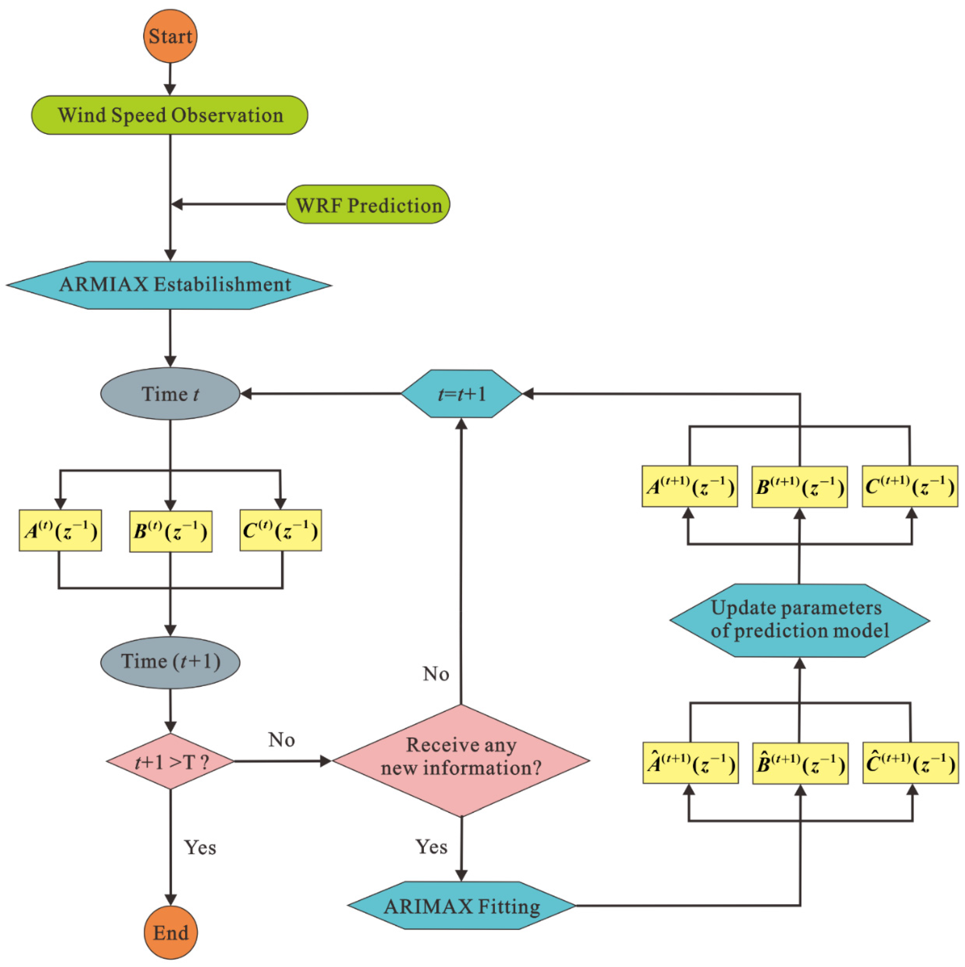
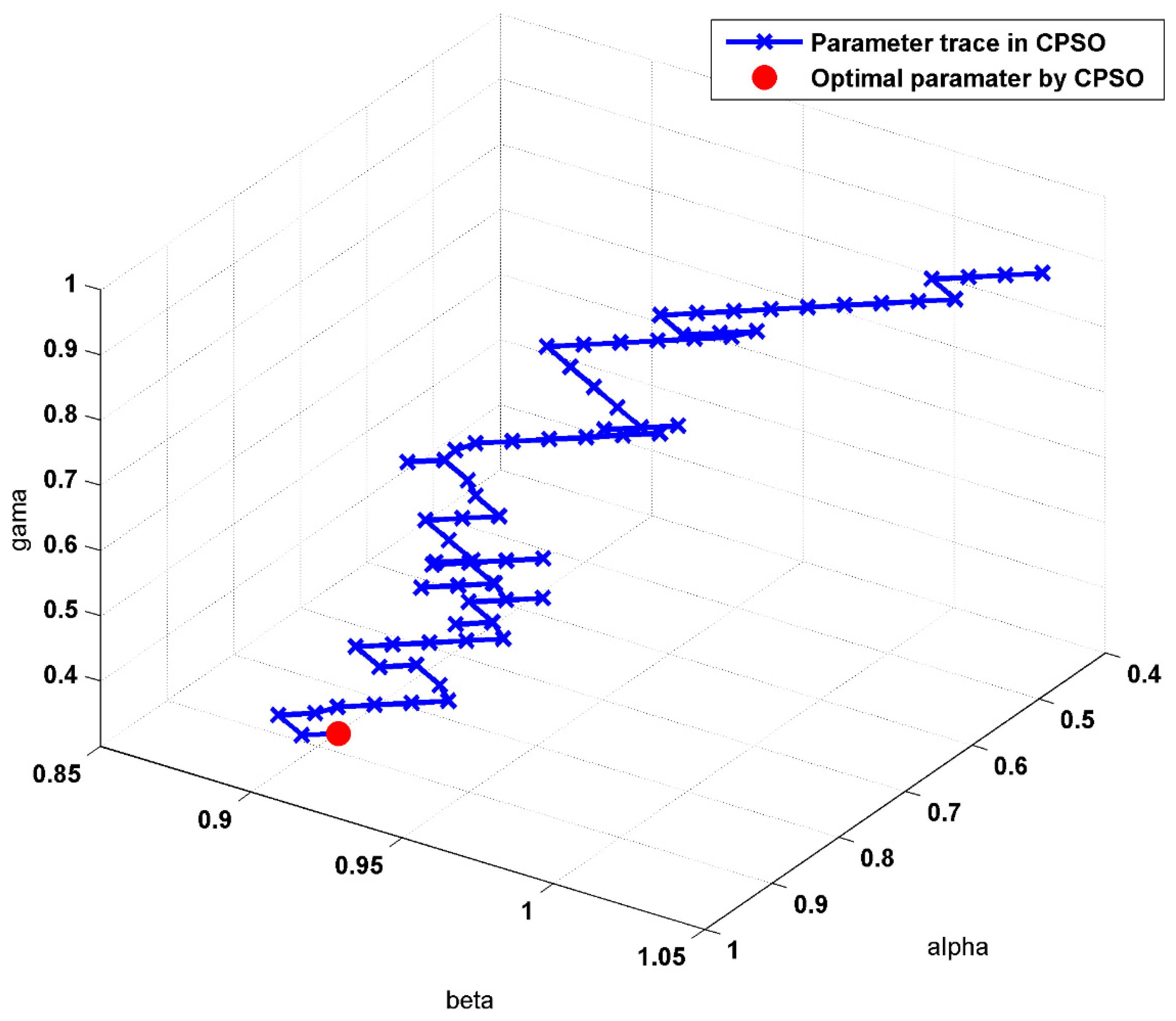
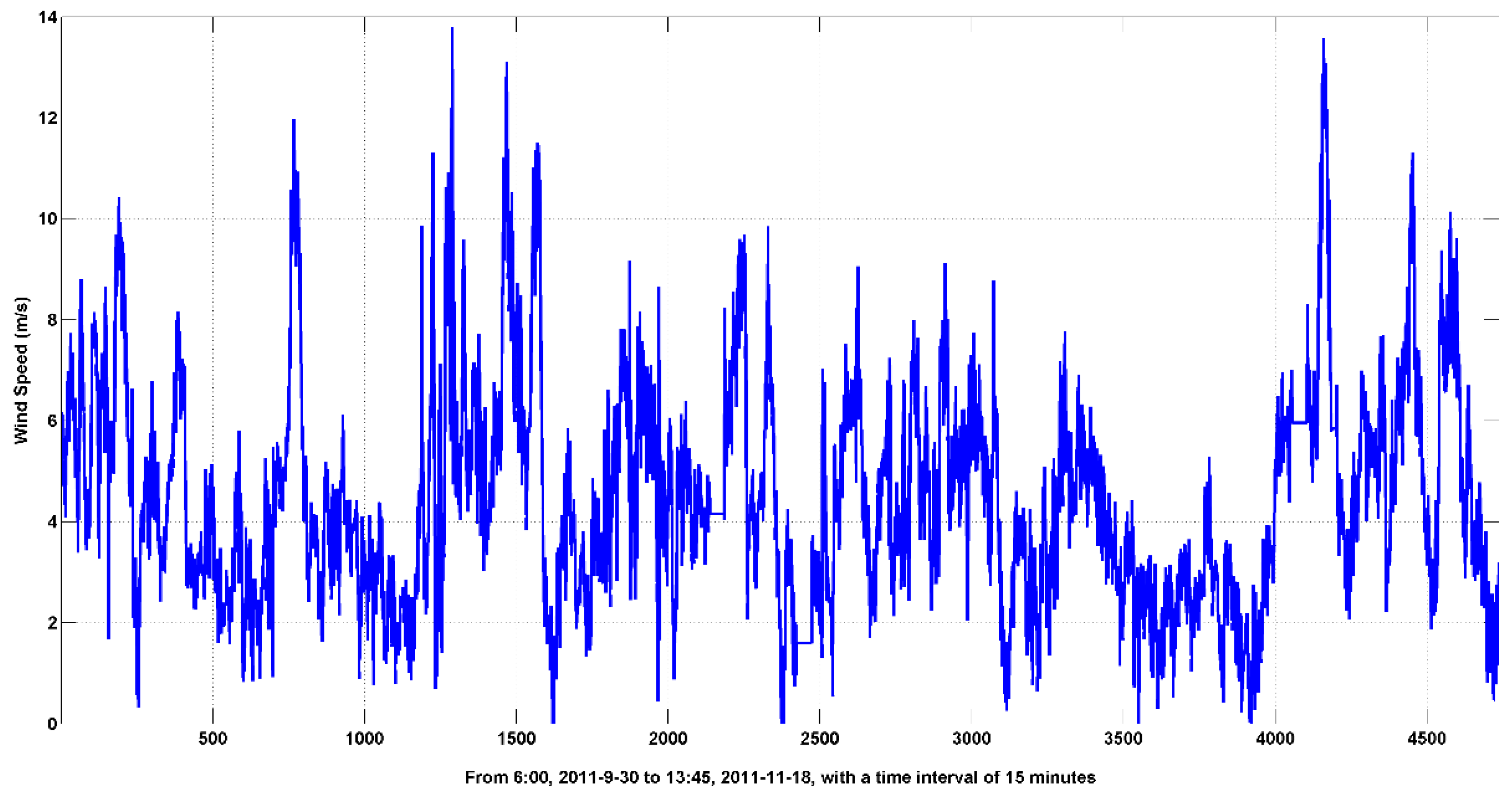
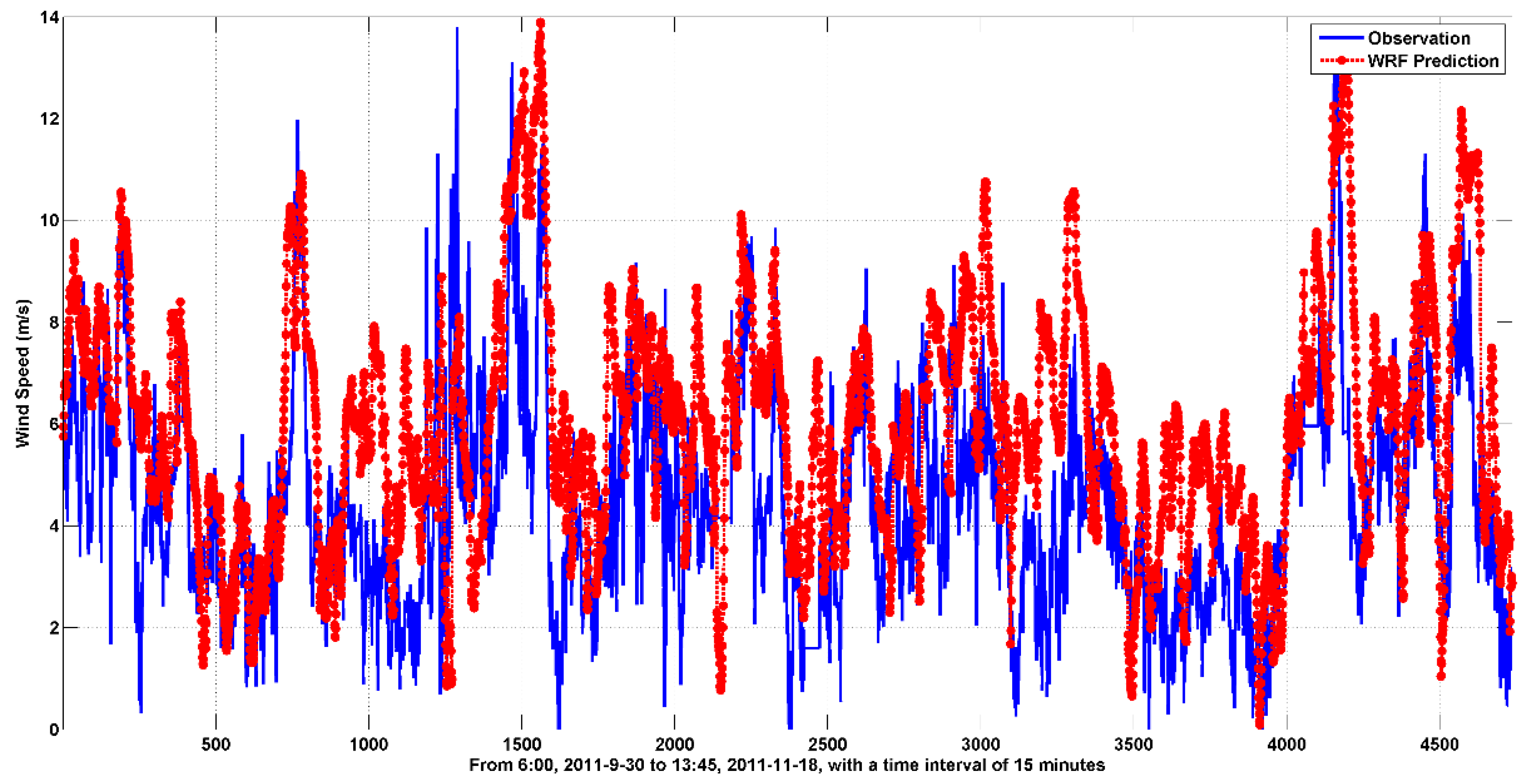
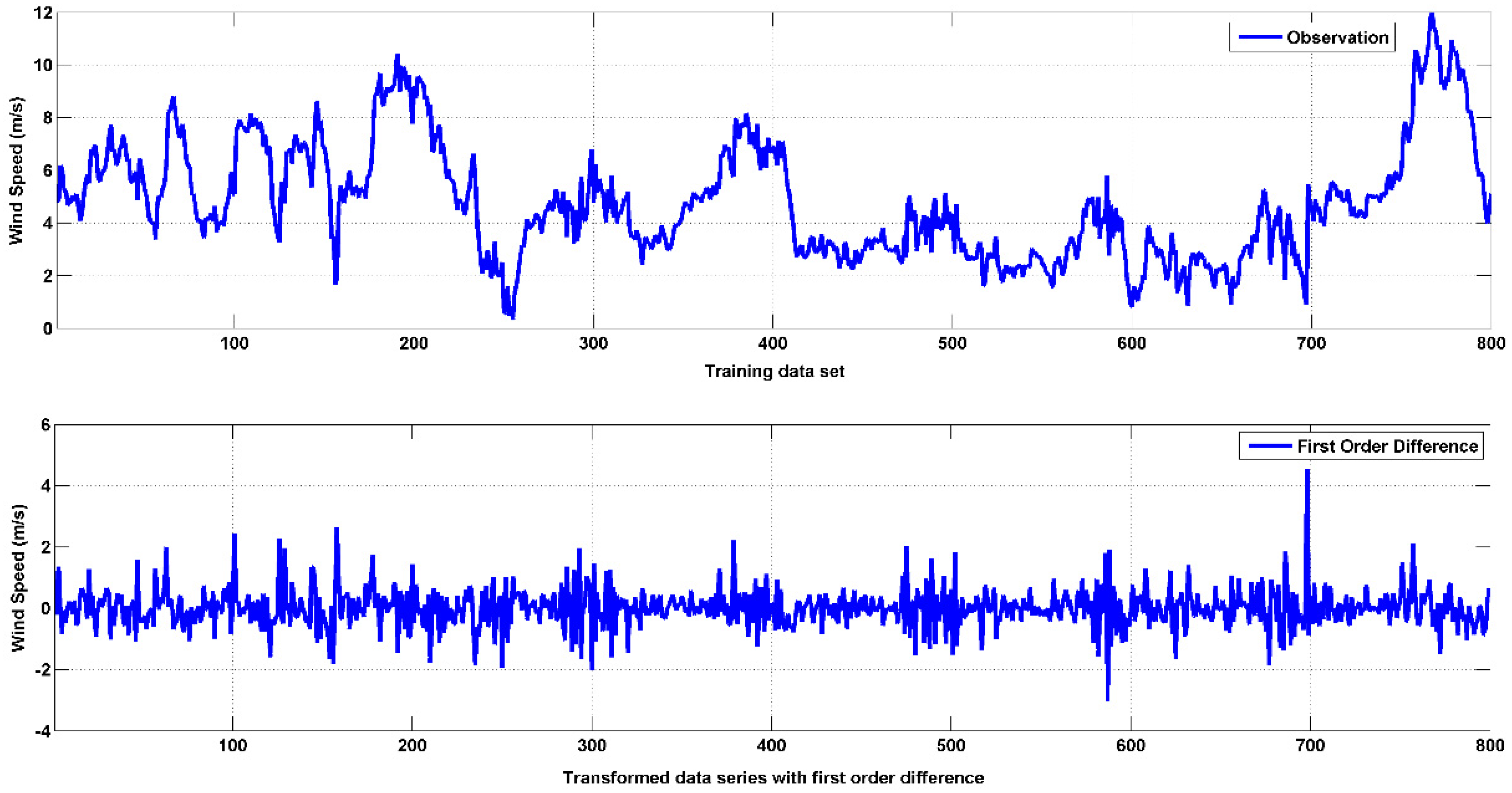
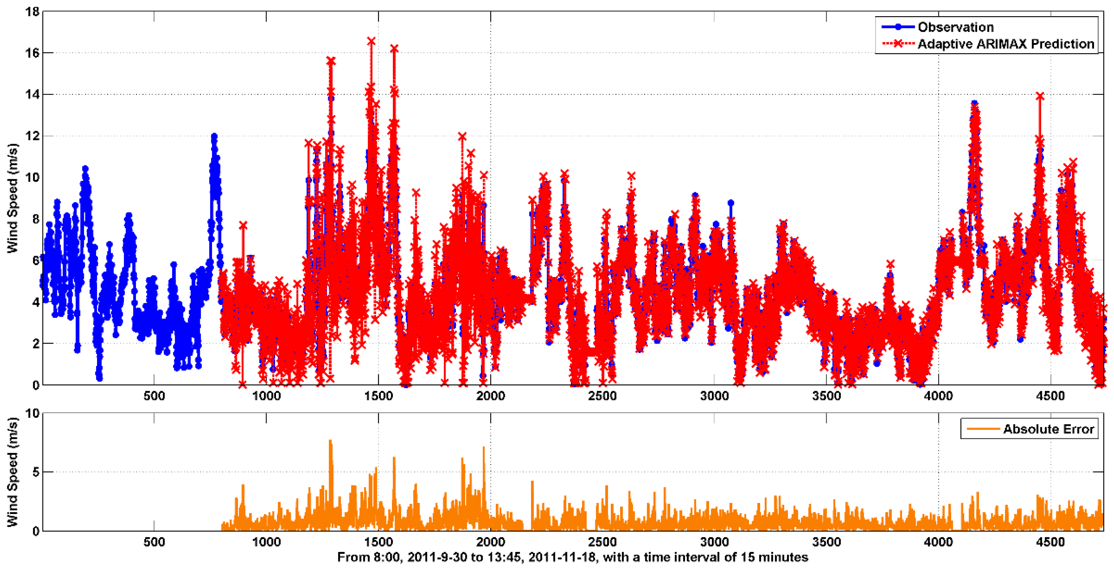
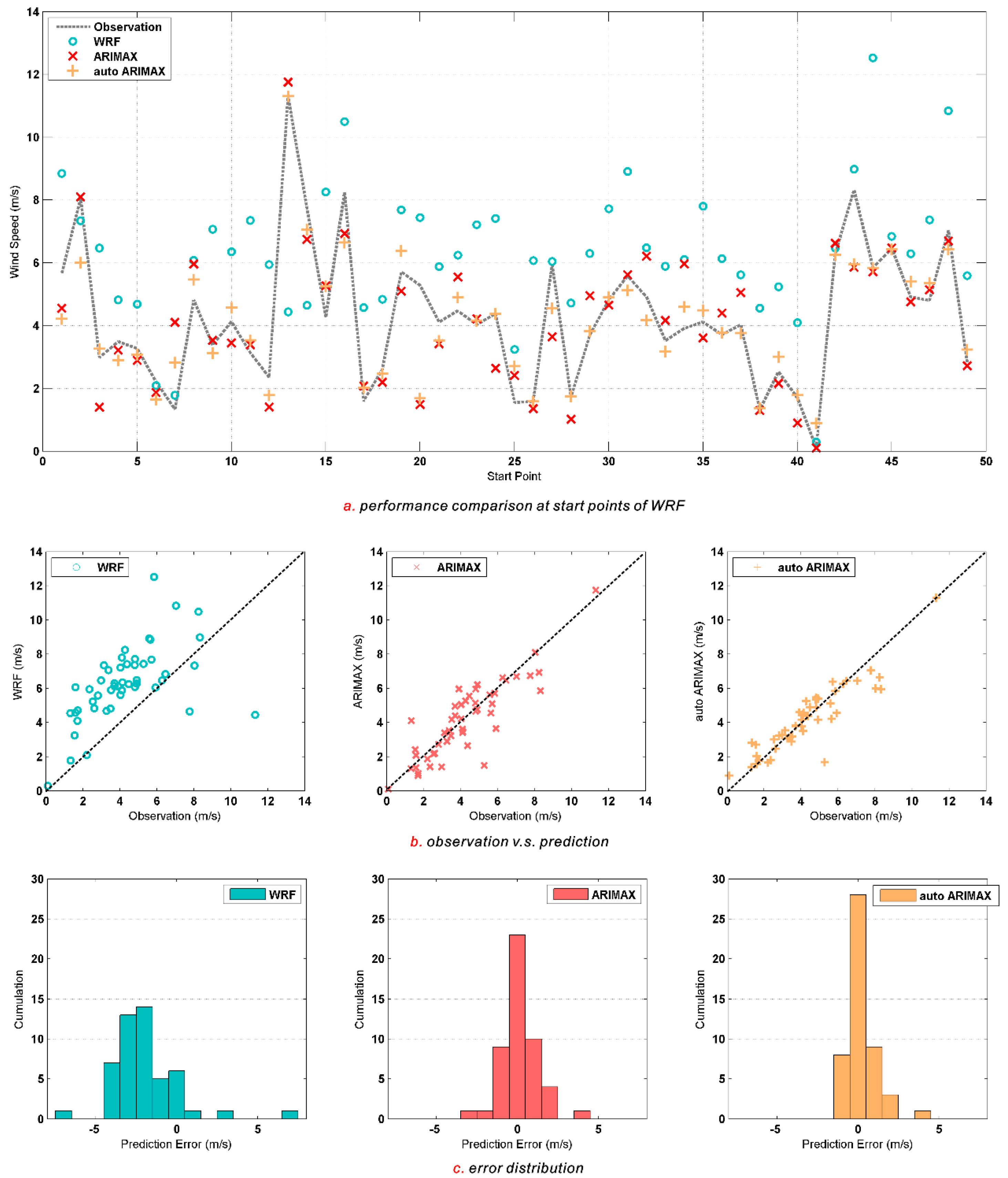
The original contribution of this paper is the development of a self-adaptive (SA) auto-regressive integrated moving average with exogenous variables (ARIMAX) model optimized by the chaotic particle swarm optimization (CPSO) algorithm called the SA-ARIMAX-CPSO approach, which is applied to wind speed prediction. Specifically, the applied ARIMAX model takes the WRF simulation as an exogenous part, which makes the forecasting model a combination of both statistical and physical information. Moreover, the CPSO-driven SA strategy enables the proposed method to syncretize the previous model and the recently updated information. In this paper, the self-adaptation contains two parts. The first one is new model fitting, when the recent measurements or WRF data are available. This paper updates the fitting coefficients every time-step, while the WRF model runs once a day. The second one is adaptation process, where the optimal adaptive weights are determined only based on the training set.

On the issue of very-short-term wind speed prediction, models were established generally based on a statistical process, while the NWP simulations were typically used for short-term predictions. This is mainly due to the model accuracy and calculation costs. This paper develops a hybrid approach for very-short-term wind speed prediction combining both statistical and physical models, which has an acceptable amount of calculation and effective model performance. Specifically, the WRF model is now the current generation physics-based atmospheric model, which is widely applied; the ARIMA process is the typical time series model, which emphasizes modelling the relationship among historical observations. Thus, the proposed ARIMAX model in this paper considers not only the statistical information from historical wind speed observations but also the physical process of atmospheric motion.

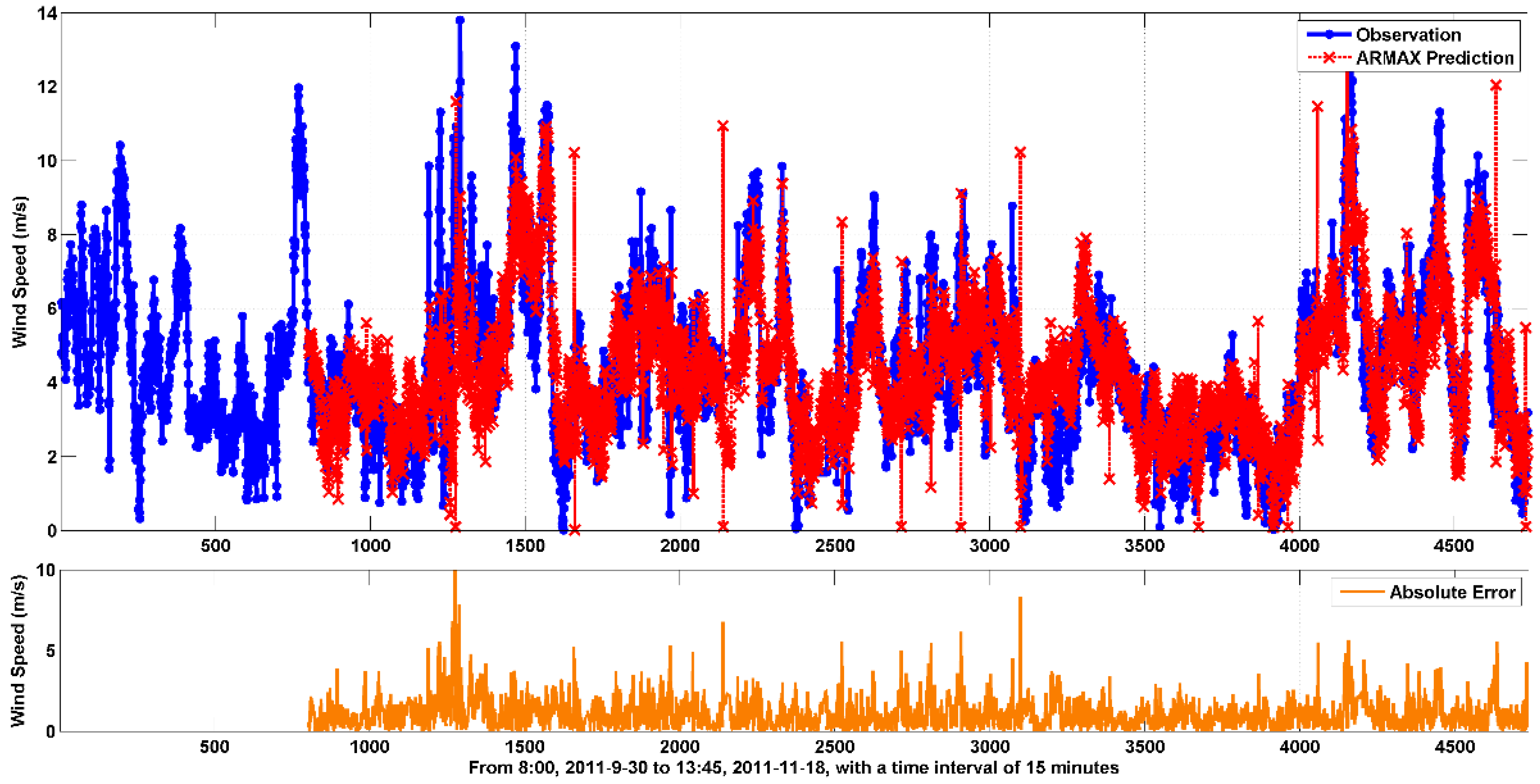
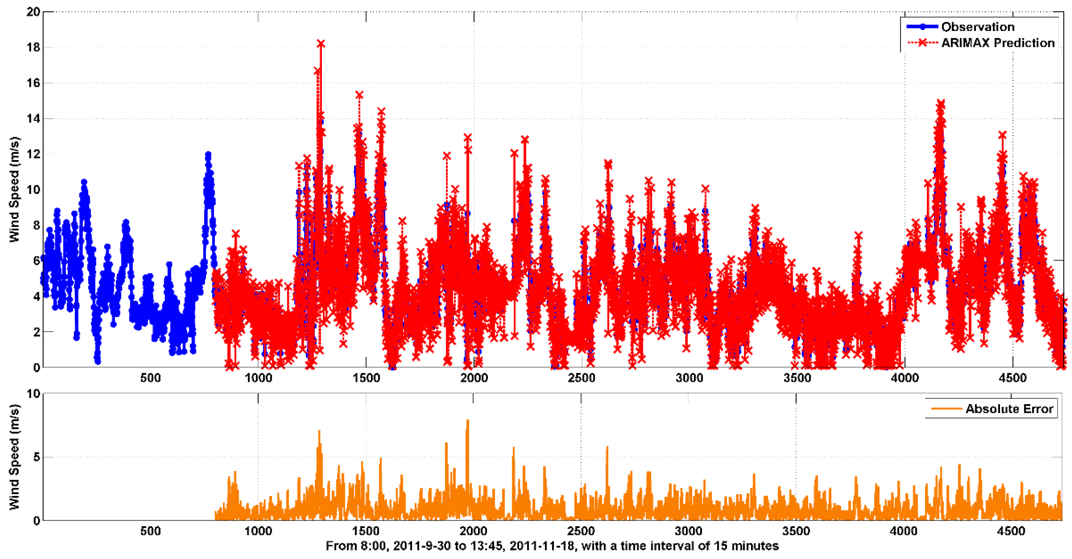
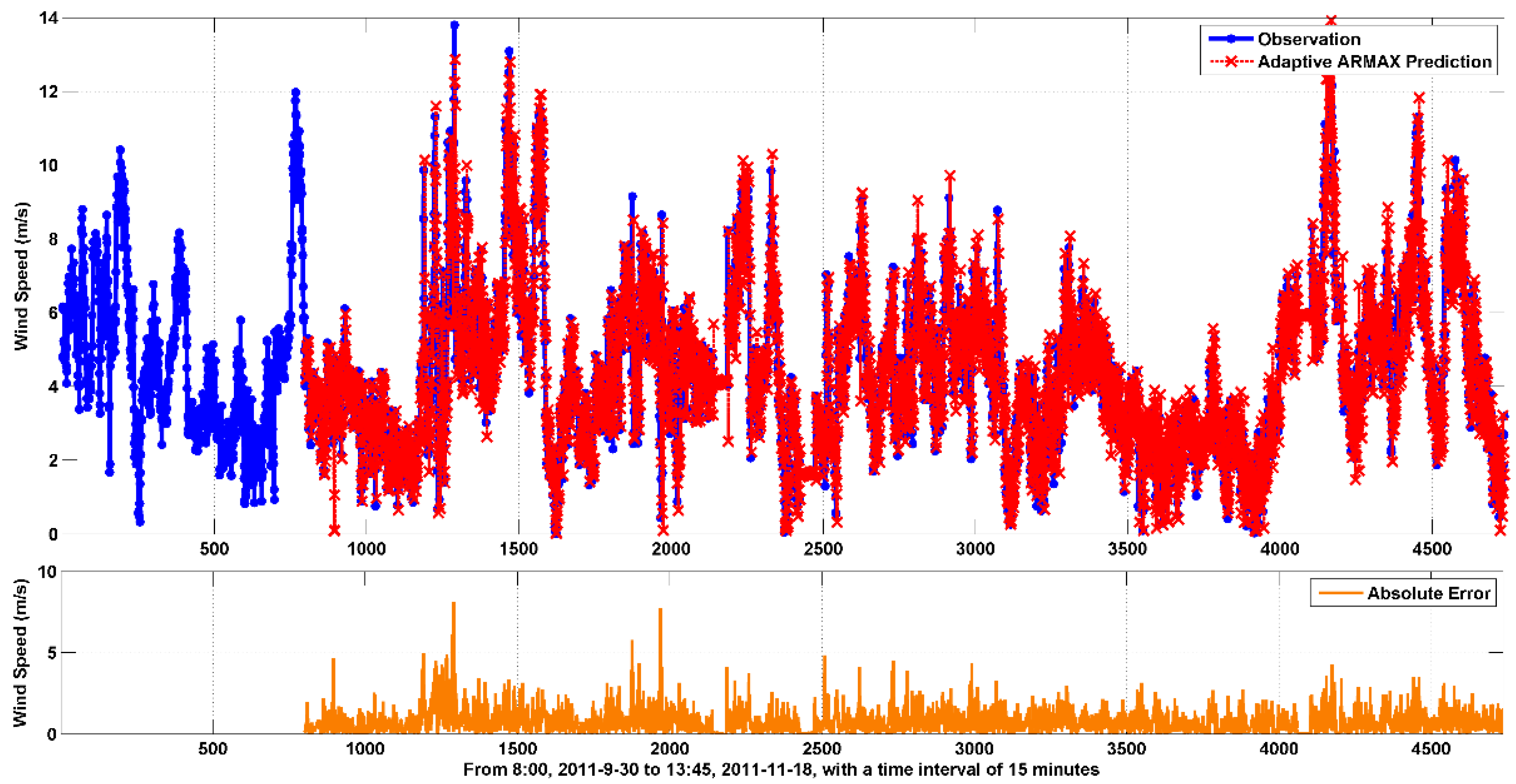
Furthermore, this paper develops a SA strategy to apply for the ARIMAX method. Model parameters are always fixed values that are determined by the training data set; this may be unreasonable in a dynamic process. When new information is obtained, the prediction system should be updated. In this paper, the new information includes two parts—the newly updated measurement records and the WRF simulation result. From this opinion, this paper develops a SA-ARIMAX model, which has adaptive model parameters when the new information is available. During this process, the CPSO algorithm is applied to obtain the optimized parameters. Simulation results show that the developed SA-ARIMAX-CPSO method in this paper performs considerably better than the original auto-regressive moving average with exogenous variables (ARMAX), ARIMAX, and adaptive ARMAX models.

1.4. Structure of This Paper

The rest of this paper is organized as follows: Section 2 reviews the original ARIMAX model. Section 3 introduces the improved SA-ARIMA optimized by the CPSO algorithm. Section 4 shows the available data sets and model measurements. Section 5 and Section 6 display the experiments and analysis. Afterward, conclusions are discussed in Section 7. Finally, acknowledgements and references are given.

2. Original ARIMAX Model

The developed ARIMAX model in this paper is a single-input and single-output (SISO) system, which is defined as follows:

$$A\left(z^{-1}\right)y\left(t\right)=B\left(z^{-1}\right)u\left(t\right)+C\left(z^{-1}\right)e\left(t\right)$$

(1)

The input data passes through a difference filter D times, where:

$$A\left(z^{-1}\right)=1-a_1{z}^{-1}-\cdots -a_p{z}^{-p}$$

(2)

$$B\left(z^{-1}\right)=b_1+b_2{z}^{-1}+\cdots +b_q{z}^{-q+1}$$

(3)

$$C\left(z^{-1}\right)=1+c_1{z}^{-1}+\cdots +c_r{z}^{-r}$$

(4)

$y\left(t\right)$ is the output at time $t$, $u\left(t\right)$ is the exogenous variable at time $t$, $e\left(t\right)$ is the white noise, and $p$, $q$ and $r$ are the orders of auto-regressive (AR), moving average (MA) and exogenous (X), respectively. Moreover, $z^{-1}$ represents the delay operator, and $A\left(z^{-1}\right)$, $B\left(z^{-1}\right)$ and $C\left(z^{-1}\right)$ are the parameters of AR, MA and X parts, respectively. It is assumed that the zero points of $A\left(z^{-1}\right)$ and $C\left(z^{-1}\right)$ are located in the unit circle. Equation (1) can be re-written as:

$$y\left(t\right)=a_{1}y\left(t-1\right)+\cdots +a_{p}y\left(t-p\right)+b_{1}u\left(t\right)+b_{2}u\left(t-1\right)+\cdots +b_{q}u\left(t-q+1\right)+e\left(t\right)+c_{1}e\left(t-1\right)+\cdots +c_{r}e\left(t-r\right)$$

(5)

To determine the model order, the most popular one is the Bayesian Information Criterion (BIC) [38]. Reference [39] provides a detailed discussion on order determination for the ARIMAX model by using the BIC method.

The parameters $A\left(z^{-1}\right)$, $B\left(z^{-1}\right)$ and $C\left(z^{-1}\right)$ are obtained by the recursive maximum likelihood estimation method [40]. Thus:

$$\theta =\left[a_1,\dots ,a_p,b_1,\dots ,b_q,c_1,\dots ,c_r\right]$$

(6)

The recursive estimation of $\theta$ can be expressed as:

$$\theta \left(t+1\right)=\theta \left(t\right)+K\left(t\right)\left(y\left(t+1\right)-{\phi }^T\left(t\right)\theta \left(t\right)\right)$$

(7)

where $\theta \left(0\right)$ can be any value, $\theta \left(i\right)=0$ if $i<0$, and:

$$K\left(t\right)=\frac{P\left(t\right)\phi \left(t\right)}{1+{\phi }^T\left(t\right)P\left(t\right)\phi \left(t\right)}$$

(8)

$$P\left(t+1\right)=P\left(t\right)-K\left(t\right){\phi }^T\left(t\right)P\left(t\right)$$

(9)

$$\phi \left(t\right)=\left[y\left(t-1\right),\dots ,y\left(t-p\right),u\left(t\right),\dots ,u\left(t-q+1\right),y\left(t-1\right)-{\phi }^T\left(t-1\right)\theta \left(t\right),\dots ,y\left(t-r\right)-{\phi }^T\left(t-r\right)\theta \left(t-r+\right)\right]$$

(10)

3. Self-Adaptive ARIMAX Optimized by CPSO Algorithm

3.1. Self-Adaptive ARIMAX (SA-ARIMAX) Method

In the original ARIMAX model introduced in Section 2, the model parameters $A\left(z^{-1}\right)$, $B\left(z^{-1}\right)$ and $C\left(z^{-1}\right)$ are fixed by the training data set. This is unreasonable in real applications. When new information is obtained, the forecast system should be updated. From this point of view, this paper develops a SA-ARIMAX model with adaptive model parameters.

The model parameters are denoted at time $t$ as $A^{\left(t\right)}\left(z^{-1}\right)$, $B^{\left(t\right)}\left(z^{-1}\right)$, and $C^{\left(t\right)}\left(z^{-1}\right)$, as follows:

$$A^{\left(t\right)}\left(z^{-1}\right)=1-a_1^{\left(t\right)}{z}^{-1}-\cdots -a_p^{\left(t\right)}{z}^{-p}$$

(11)

$$B^{\left(t\right)}\left(z^{-1}\right)=b_1^{\left(t\right)}+b_2^{\left(t\right)}{z}^{-1}+\cdots +b_q^{\left(t\right)}{z}^{-q+1}$$

(12)

$$\phi C^{\left(t\right)}\left(z^{-1}\right)=1+c_1^{\left(t\right)}{z}^{-1}+\cdots +c_r^{\left(t\right)}{z}^{-r}$$

(13)

Assuming that the model parameters at time $t$ are estimated, Equation (5) can be re-rewritten as:

$$\widehat{y}(t+1)=a_1^{\left(t\right)}y\left(t\right)+\dots +a_p^{\left(t\right)}y(t-p+1)+b_1^{\left(t\right)}u(t+1)+b_2^{\left(t\right)}u\left(t\right)+\dots +b_q^{\left(t\right)}u(t-p+2)+e(t+1)+c_1^{\left(t\right)}e\left(t\right)+\dots +c_r^{\left(t\right)}e(t-r+1)$$

(14)

When the new information is obtained at time $\left(t+1\right)$, the model parameters should be updated. As fitted by ARIMAX with the same model orders as previously stated, parameters are obtained and denoted as ${\widehat{A}}^{\left(t\right)}\left(z^{-1}\right)$, ${\widehat{B}}^{\left(t\right)}\left(z^{-1}\right)$, and ${\widehat{C}}^{\left(t\right)}\left(z^{-1}\right)$. Then, at time $\left(t+1\right)$, the parameters of the forecasting model should be influenced not only by the parameters at time $t$, $A^{\left(t\right)}\left(z^{-1}\right)$, $B^{\left(t\right)}\left(z^{-1}\right)$, and $C^{\left(t\right)}\left(z^{-1}\right)$ but also by the new information ${\widehat{A}}^{\left(t\right)}\left(z^{-1}\right)$, ${\widehat{B}}^{\left(t\right)}\left(z^{-1}\right)$, and ${\widehat{C}}^{\left(t\right)}\left(z^{-1}\right)$. Thus, this paper takes a weighted average of the two aspects, as:

$$A^{\left(t+1\right)}\left(z^{-1}\right)=\left(1-\alpha \right){\widehat{A}}^{\left(t+1\right)}\left(z^{-1}\right)+\alpha A^{\left(t\right)}\left(z^{-1}\right)$$

(15)

$$B^{\left(t+1\right)}\left(z^{-1}\right)=\left(1-\beta \right){\widehat{B}}^{\left(t+1\right)}\left(z^{-1}\right)+\beta B^{\left(t\right)}\left(z^{-1}\right)$$

(16)

$$C^{\left(t+1\right)}\left(z^{-1}\right)=\left(1-\gamma \right){\widehat{C}}^{\left(t+1\right)}\left(z^{-1}\right)+\gamma C^{\left(t\right)}\left(z^{-1}\right)$$

(17)

where $0<\alpha ,\beta ,\gamma <1$ are three weights.

3.2. Parameters in the SA-ARIMAX Model

There are two categories of parameters in the SA-ARIMAX model. One category are the ARIMAX parameters, named $A\left(z^{-1}\right)$, $B\left(z^{-1}\right)$ and $C\left(z^{-1}\right)$ and defined by Equations (11)–(13). This set of parameters can always be obtained by the least square (LS) method during the model fitting process. The other category is the self-adaptive parameters, $\alpha ,\beta ,\text{\hspace{0.17em}and\hspace{0.17em}}\gamma$, defined in Equations (15)–(17) when applying the SA strategy to an ARIMAX process. It can be easily found that parameters $\alpha ,\beta ,\text{\hspace{0.17em}and\hspace{0.17em}}\gamma$ represent a weighted average between the historical and the newly fitted model parameters. Larger $\alpha ,\beta ,\text{\hspace{0.17em}and\hspace{0.17em}}\gamma$prove that the prediction model takes more information from the historical model parameters, while smaller values of $\alpha ,\beta ,\text{\hspace{0.17em}and\hspace{0.17em}}\gamma$prove that the newly fitted model parameters cause more influence on the final forecasting results.

Values of $\alpha ,\beta ,\text{\hspace{0.17em}and\hspace{0.17em}}\gamma$ affect the model performance by constructing a different information balance between the historical and newly fitted model parameters. The determination of $\alpha ,\beta ,\text{\hspace{0.17em}and\hspace{0.17em}}\gamma$ is difficult but quite essential. To search for the optimized parameters $\alpha ,\beta ,\text{\hspace{0.17em}and\hspace{0.17em}}\gamma$ during the SA process, this paper applies the CPSO algorithm, which is a swarm intelligent method. The combination with the CPSO algorithm enables the developed SA-ARIMAX model to absorb the newly updated information with an optimized coefficient.

3.3. Model Optimization by CPSO Algorithm

3.3.1. Working Principle of CPSO Algorithm

Particle swarm optimization (PSO) simulates the social psychological metaphor based on swarm intelligence. Two best values exist in the simulation process of PSO. For each particle in the problem space, the best value obtained up to now is denoted as $pBest$. In terms of the global version, the overall best solution achieved up to now is called $gBest$. The procedure for PSO can be expressed as shown in Appendix A [41,42].

3.3.2. Developed Method: SA-ARIMAX Optimized by CPSO (SA-ARIMAX-CPSO)

In this paper, the three coefficients, $\alpha ,\beta ,\text{\hspace{0.17em}and\hspace{0.17em}}\gamma$, are optimized by the CPSO algorithm introduced in Section 3.3.1. Then, the prediction value at time $\left(t+1\right)$ can be calculated by Equation (14) using the optimized parameters. The developed self-adaptive ARIMAX method optimized by CPSO, called SA-ARIMAX-CPSO in this paper, can be divided into several steps as Appendix B shows. Figure 1 shows the flowchart.

Figure 1. The flow chart of SA-ARIMAX-CPSO method.

Figure 1. The flow chart of SA-ARIMAX-CPSO method.

In practice, the new information is not updated at every time $t$, thus the model parameters should be updated when the new information, newly-obtained observation or WRF simulation data, is available. This forecasting process could be concluded as follows: assuming that $t+1<T$ and the parameters at time $t$, $A^{\left(t\right)}\left(z^{-1}\right)$, $B^{\left(t\right)}\left(z^{-1}\right)$, and $C^{\left(t\right)}\left(z^{-1}\right)$, are obtained. Thus, the parameters at time $\left(t+1\right)$ can be calculated:

$$A^{\left(t+1\right)}\left(z^{-1}\right)=\{\begin{array}{c}{A}^{\left(t\right)}\left(z^{-1}\right),\text{\hspace{0.17em}if\hspace{0.17em}no\hspace{0.17em}new\hspace{0.17em}information\hspace{0.17em}is\hspace{0.17em}received}\hfill \\ \left(1-\alpha \right){\widehat{A}}^{\left(t+1\right)}\left(z^{-1}\right)+\alpha A^{\left(t\right)}\left(z^{-1}\right),\text{\hspace{0.17em}otherwise}\hfill \end{array}$$

(18)

$$B^{\left(t+1\right)}\left(z^{-1}\right)=\{\begin{array}{c}{B}^{\left(t\right)}\left(z^{-1}\right),\text{\hspace{0.17em}if\hspace{0.17em}no\hspace{0.17em}new\hspace{0.17em}information\hspace{0.17em}is\hspace{0.17em}received}\hfill \\ \left(1-\beta \right){\widehat{B}}^{\left(t+1\right)}\left(z^{-1}\right)+\beta B^{\left(t\right)}\left(z^{-1}\right),\text{\hspace{0.17em}otherwise}\hfill \end{array}$$

(19)

$$C^{\left(t+1\right)}\left(z^{-1}\right)=\{\begin{array}{c}{C}^{\left(t\right)}\left(z^{-1}\right),\text{\hspace{0.17em}if\hspace{0.17em}no\hspace{0.17em}new\hspace{0.17em}information\hspace{0.17em}is\hspace{0.17em}received}\hfill \\ \left(1-\gamma \right){\widehat{C}}^{\left(t+1\right)}\left(z^{-1}\right)+\gamma C^{\left(t\right)}\left(z^{-1}\right),\text{\hspace{0.17em}otherwise}\hfill \end{array}$$

(20)

where ${\widehat{A}}^{\left(t+1\right)}\left(z^{-1}\right)$, ${\widehat{B}}^{\left(t+1\right)}\left(z^{-1}\right)$, and ${\widehat{C}}^{\left(t+1\right)}\left(z^{-1}\right)$ represent the new information.

3.3.3. How the CPSO Works: An AI-Based Optimization Process

As introduced in Section 3, the CPSO algorithm is employed as a parameter searching tool, optimizing the parameters $\alpha ,\beta ,\text{\hspace{0.17em}and\hspace{0.17em}}\gamma$ in Equations (15)–(17). This section aims to display how the parameters $\alpha ,\beta ,\text{\hspace{0.17em}and\hspace{0.17em}}\gamma$ are optimized during a CPSO-driven process. The maximum iteration is set as 100; Figure 2 displays the parameter values for each iteration.

The CPSO-driven optimization process is a parameter searching process, promoting the reduction of the fitness value. For each step, the best values, $pBest$ and $gBest$, will be updated if the fitness value meets a better value, which means a lower fitness value in this study. Figure 2 shows the parameter changing trace, where alpha, beta, gamma imply $\alpha ,\beta ,\text{\hspace{0.17em}and\hspace{0.17em}}\gamma$, respectively. Denote the $t$-th iteration of $\alpha ,\beta ,\text{\hspace{0.17em}and\hspace{0.17em}}\gamma$ as $x\left(t\right)=\left(x_1\left(t\right),x_2\left(t\right),x_3\left(t\right)\right)$. Then, the $\left(t+1\right)$-th iteration can be expressed as:

$$v\left(t+1\right)=w·v\left(t\right)+c_1·uD\left(t\right)·\left[pBest\left(t\right)-x\left(t\right)\right]+c_2·UD\left(t\right)·\left[gBest\left(t\right)-x\left(t\right)\right]$$

(21)

$$x\left(t+1\right)=x\left(t\right)+\Delta t·v\left(t+1\right)$$

(22)

where $w$ is the parameter called inertia weight, $c_1$ and $c_2$ are positive constants, $\text{and }uD$ and $UD$ are random figures uniformly distributed in $\left[0,1\right]$. Thus, the vector $v$ can be regarded as the velocity vector of the parameter iteration. Then, the position $x\left(t+1\right)$ can be calculated by adding the velocity vector $v\left(t+1\right)$ onto the previous position $x\left(t\right)$, where $\Delta t$ means the step length.

To strengthen the randomness, different combination methods regarding parameters were given [43]. In this paper, $w$ is iterated by the following Tent Map:

$$w\left(t+1\right)=\{\begin{array}{c}\frac{w\left(t\right)}{0.7},w\left(t\right)<0.7\\ \frac{10}{3w\left(t\right)\left(1-w\left(t\right)\right)},w\left(t\right)\ge 0.7\end{array}$$

(23)

$$w\left(t+1\right)=w\left(t+1\right)+0.5$$

(24)

$c_1$ and $c_2$ are updated by the Logistic Map:

$$c_1\left(t+1\right)=a·c_1\left(t\right)\left(1-c_1\left(t\right)\right)$$

(25)

$$c_2\left(t+1\right)=a·c_2\left(t\right)\left(1-c_2\left(t\right)\right)$$

(26)

where, generally, $a=4$, $c_1,c_2\in \left(0,1\right)$.

Figure 2. Trace of parameters during a CPSO-driven process.

Figure 2. Trace of parameters during a CPSO-driven process.

4. Available Data Sets

This study site is a wind farm in Shandong Province in Northern China. Figure 3 shows the topography of Shandong Province and the location of the study site. The data set used in this paper was collected from an anemometer tower located in the range of this wind farm, which measuring height is 70 m. The available data are from 6:00, 2011-9-30 to 13:45, 2011-11-18, with a time interval of 15 min (Figure 4) There are 3.26% missing data, and the missing data are filled by linear interpolation. Table 1 shows the basic statistical description of the available data. Moreover, Figure 5 displays the frequency distribution of the available data and the probability distribution function (pdf) fitted by the two-parameter Weibull distribution:

$$f\left(v\right)=\frac{k}{c}{\left(\frac{v}{c}\right)}^{k-1}exp\left[-{\left(\frac{v}{c}\right)}^k\right],v\ge 0$$

(27)

where $k$ and $c$ are the shape parameter and scale parameter, respectively, and $v$ represents the wind speed records. Applying the maximum likelihood (ML) method, the shape and scale parameters are 5.0258 and 2.1490, respectively.

Figure 3. The topography of Shandong Province.

Figure 3. The topography of Shandong Province.

Figure 4. The available data.

Figure 4. The available data.

Table 1. Statistical description of available data.

Number	Minimum (m/s)	Maximum (m/s)	Mean (m/s)	Standard Deviation	Skewness	Kurtosis
5000	0.1	13.8	4.29	2.23	0.74	0.69

Table 1. Statistical description of available data.

Number	Minimum (m/s)	Maximum (m/s)	Mean (m/s)	Standard Deviation	Skewness	Kurtosis
5000	0.1	13.8	4.29	2.23	0.74	0.69

Figure 5. Frequency distribution of the available data.

Figure 5. Frequency distribution of the available data.

5. Experiments and Analysis

Experiments in this paper are composed of three parts. The first part displays the WRF configuration and prediction, which will be used as an exogenous input in the following model construction. Then, the second part discusses the original ARMAX and ARIMAX predictions. This part aims to test the model performance without the SA strategy, which means the fixed model parameters will be used during the whole tested period. After that, the developed SA strategy is applied, with the same model setup as the original ARMAX and ARIMAX models.

5.1. WRF Meso-Scale Numerical Model Prediction

The WRF meso-scale numerical model is now the current generation physics-based atmospheric model, serving the needs of both atmospheric research and operational forecasting. Recently, the WRF model has become one of the most popular and widely used tools for numeric weather prediction. In this paper, the WRF model is selected as a representative for the physical models.

The WRF model domain has 150 by 120 horizontal grid points, spaced at 27 km, situated on 47 terrain following vertical levels. In the WRF model, a grid is defined as an integration of three dimensional points. It contains a set of weather data (wind speed, atmospheric pressure etc.). Physical equations are used to simulate the atmospheric state; this is based not only on the data on grid but also a specific physical model. Then, the simulations are calculated by discretized time-steps [44].

In the developed ARIMAX model, a wind speed prediction from the WRF simulation is adopted as an exogenous variable. First, this section provides the WRF results. The initial and boundary conditions of the WRF simulation are extracted from the National Centres for Environmental Prediction (NCEP, http://www.ncep.noaa.gov/) reanalysis data (1°×1°); the time resolution is 15 min, and the spatial resolution is 27 km. The physical options of the WRF model are described in Table 2. The WRF calculation discussed in this paper is a one-day simulation, which starts at 8:00 am (China Standard Time, CST) on the first day to 8:00 am (CST) on the second day.

Table 2. Model configuration of WRF simulation.

	Physical Options
Cumulus parameterization	Grell 3d ensemble cumulus scheme
Longwave/Shortwave radiation	RRTM/Dudhia scheme
Surface layer physics	Eta similarity
Land surface processes	Noah Land Surface Model
Planetary Boundary layer	Mellor-Yamada-Janjic scheme

Table 2. Model configuration of WRF simulation.

	Physical Options
Cumulus parameterization	Grell 3d ensemble cumulus scheme
Longwave/Shortwave radiation	RRTM/Dudhia scheme
Surface layer physics	Eta similarity
Land surface processes	Noah Land Surface Model
Planetary Boundary layer	Mellor-Yamada-Janjic scheme

Figure 6 shows the WRF prediction in the experimental period. It is clear that the WRF prediction can describe the overall variability of wind speed, even though the forecasting accuracy should be enhanced. The atmospheric dynamics information plays an important role in WRF prediction. In the next section, this result will be an exogenous input of the ARIMAX model; it is regarded as a reference value for the final prediction. Thus, the developed prediction procedure contains information not only from historical observations but also from physical-based WRF results.

Figure 6. The WRF prediction in the study period.

Figure 6. The WRF prediction in the study period.

5.2. Original ARMAX and ARIMAX Predictions

This section establishes the original ARIMAX model. The first 800 observations of the available data set are chosen as the initial training data set; the rest is used for rolling prediction and model testing. By using the BIC method, ARMAX (3,3,1) is established. Figure 7 shows the ARMAX results and absolute error. The absolute error of the ARMAX prediction is mainly distributed in a range of 0 to 4 m/s. The original ARMAX model has high MAPE in wind speed prediction. This may result from two aspects. One aspect is the strong fluctuation of the wind speed time series, which makes it difficult to capture the variation and randomness. The other aspect may be the fixed model parameters in the original ARMAX model.

Figure 7. ARMAX prediction results.

Figure 7. ARMAX prediction results.

To transform the original observation data into a stationary sequence, the first-order difference is adopted; therefore, the ARIMAX model is established. Figure 8 shows the transformed data series, and Figure 9 provides the ARIMAX predictions. Compared with Figure 7, the ARIMAX prediction has fewer statistical errors and this phenomenon also occurs in Table 3, which provides detailed error comparisons among the root mean absolute error (RMSE), Bias and correlation coefficient (R). Compared with ARMAX prediction, the ARIMAX model has a decline of 14.69% in RMSE.

At the same time, it can also be found from Figure 9 that the ARIMAX prediction has a strong fluctuation, and the predicted value is always considerably higher than the observation. Therefore, the model performance should be improved further. In the following sections, a method of adaptive model parameters is applied to both ARMAX and ARIMAX procedures. Simulation results show that predictions with adaptive parameters perform considerably better than the original ARMAX and ARIMAX predictions.

Figure 8. Transformed data set with first order difference.

Figure 8. Transformed data set with first order difference.

Figure 9. ARIMAX prediction results.

Figure 9. ARIMAX prediction results.

Table 3. Errors of ARMAX and ARIMAX models.

	RMSE (m/s)	Bias (m/s)	R
ARMAX	1.43	−0.10	0.76
ARIMAX	1.22	0.04	0.87

Table 3. Errors of ARMAX and ARIMAX models.

	RMSE (m/s)	Bias (m/s)	R
ARMAX	1.43	−0.10	0.76
ARIMAX	1.22	0.04	0.87

5.3. Developed SA-ARMAX-CPSO and SA-ARIMAX-CPSO Predictions

In this section, this paper develops a method of adaptive parameters. The developed method is applied to both SA-ARMAX and SA-ARIMAX procedures. The three weights, $\alpha$, $\beta$, and $\gamma$, are obtained by the CPSO algorithm, as $\alpha =0.96$, $\beta =0.92$, $\gamma =0.39$. Figure 10 and Figure 11 show the prediction results.

Figure 10. Adaptive ARMAX prediction results.

Figure 10. Adaptive ARMAX prediction results.

Compared to Figure 7 and Figure 9, the adaptive models show significant improvements. Table 4 shows the detailed statistical errors of the adaptive ARMAX and adaptive ARIMAX models. The adaptive ARIMAX model performs slightly better than the adaptive ARMAX model, which can be found from all three criteria in Table 4.

Figure 11. Adaptive ARIMAX prediction results.

Figure 11. Adaptive ARIMAX prediction results.

However, compared with the original ARMAX and ARIMAX predictions, adaptive models work more efficiently. Specifically, when compared with the original ARMAX/ARIMAX models, the SA-ARMAX/ARIMAX-CPSO models show 23.78% and 12.30% lower RMSE, respectively. Bias of the adaptive methods declines and the correlation coefficients of the adaptive methods increase, compared with the original ARMAX/ARIMAX models. This is a benefit of the CPSO-driven SA strategy proposed in this paper. It indicates that the developed adaptive method effectively improves the original model performances.

Table 4. Errors of adaptive ARMAX and adaptive ARIMAX models.

	RMSE (m/s)	Bias (m/s)	R
Adaptive ARMAX	1.09	−0.05	0.87
Adaptive ARIMAX	1.07	0.03	0.89

Table 4. Errors of adaptive ARMAX and adaptive ARIMAX models.

	RMSE (m/s)	Bias (m/s)	R
Adaptive ARMAX	1.09	−0.05	0.87
Adaptive ARIMAX	1.07	0.03	0.89

5.4. Performance Comparison among Several Models

This paper employs the WRF model as an exogenous input to the ARMA/ARIMA methods, where this physical model runs once a day. Thus, it is significant to compare the model performance between the WRF and ARMAX/ARIMAX models at the start point of WRF prediction, which is 8:00 am CST in this paper. Figure 12 displays the comparison results among them.

Figure 12. Performance comparison among WRF, ARIMAX and adaptive ARIMAX. (a) Performance comparison at start points of WRF; (b) Observation vs. prediction; (c) Error distribution.

Figure 12. Performance comparison among WRF, ARIMAX and adaptive ARIMAX. (a) Performance comparison at start points of WRF; (b) Observation vs. prediction; (c) Error distribution.

Specifically, Figure 12a shows the observation and different predictions at the starting point of the WRF model. It can be found that no model always performs its best at each start point. Figure 12b contains three scatter plots between the observation and three different predictions. The smaller distance between the scatter points and the fixed line ($y=x$) refers to the better performance of the forecasting model. Obviously, the adaptive ARIMAX model shows the best performance among the three models. This can also be found in the Figure 12c, which displays the histogram for the forecasting error. The error distribution of WRF is wider than the other two, which indicates that the WRF simulation may have bad performances in some cases. This is disadvantageous when considering the very-short-term wind speed prediction. Different from it, the ARIMAX and adaptive ARIMAX models use the WRF prediction as an exogenous input; thus, the physical simulation can be a reference value to the final result. The error distribution of the adaptive ARIMAX model concentrates around zero value, which implies that the self-adaptive method is more stable and effective. Moreover, the comparison also indicates that although the physical prediction is regarded as a reference value, the final result of the ARIMAX prediction is not totally driven by the WRF simulation. The model performance benefits from both physical and statistical model processes. This can be also found in Table 5, which displays the comparison among WRF, ARIMAX and adaptive ARIMAX at the starting points of WRF simulation.

Table 5. Errors comparison at the starting points of WRF simulation.

	RMSE (m/s)	Bias (m/s)	R
WRF	2.54	1.61	0.57
ARIMAX	1.12	−0.14	0.87
Adaptive ARIMAX	0.91	−0.15	0.91

Table 5. Errors comparison at the starting points of WRF simulation.

	RMSE (m/s)	Bias (m/s)	R
WRF	2.54	1.61	0.57
ARIMAX	1.12	−0.14	0.87
Adaptive ARIMAX	0.91	−0.15	0.91

6. Further Discussions

The simulation in Section 5.2 shows that the proposed adaptive ARIMAX method performs better than the adaptive ARMAX and the original ARIMAX models, with a lower value of statistical errors. To provide a deeper understanding of how the forecasting errors can be reduced by the proposed method, this section has an additional discussion on this topic from the following aspects.

6.1. Contribution of the CPSO-Driven SA Strategy: Reduce the Forecasting Errors

As mentioned above, the principle of the proposed SA strategy is a combination of the historical model and the recently updated information, and the three parameters $\alpha ,\beta ,\text{\hspace{0.17em}and\hspace{0.17em}}\gamma$ determine the weight of this balance. The simulation result indicates that the CPSO-driven SA strategy contributes to the reduction of model errors.

• Contribution of the SA strategy. As well known, statistical models are established by finding the relationships inside the data records. An intuitionistic idea is that the newly fitted model contains the recently updated information and always leads to better results. However, series such as wind speed show continuous changes and strong variations, and the WRF simulation also contains unavoidable uncertainties itself. All of these factors may result in poor model performance. Thus, a combination of both the historical model and the recently updated information makes the forecasting process more stable.
• Contribution of the CPSO-driven optimization. Concerning the SA strategy, the most important task is to determine the balance between the historical model and the newly fitted model, which means the parameters $\alpha ,\beta ,\text{\hspace{0.17em}and\hspace{0.17em}}\gamma$. Larger $\alpha ,\beta ,\text{\hspace{0.17em}and\hspace{0.17em}}\gamma$ prove that the model takes more information from the historical form, whereas the smaller values indicate the newly fitted model brings more influence. Under this circumstance, the CPSO algorithm is employed as a parameter searching tool to find the optimal value in the meaning of artificial intelligence.

6.2. Discussion on the Optimized Parameters

The optimal values are not identical for the three parameters. In this paper, the CPSO-driven optimal values of $\alpha ,\beta ,\text{\hspace{0.17em}and\hspace{0.17em}}\gamma$ are 0.96, 0.92, and 0.39, respectively. These three values are not identical, which means the three parts in an ARIMAX model, AR, MA, and X, perform in different ways.

• The CPSO-driven optimal values of $\alpha$ and $\beta$ are similar. Taking $\alpha =0.96$ as an example, it means that $A^{\left(t+1\right)}\left(z^{-1}\right)$ is nearly equal to $A^{\left(t\right)}\left(z^{-1}\right)$, and ${\widehat{A}}^{\left(t+1\right)}\left(z^{-1}\right)$ only contributes to a very small percentage. A comparable discussion can be given for the parameter $\beta$. This indicates that the AR and MA parts heavily rely on the historical model parameters but not the recently updated model information.
• Different from $\alpha$ and $\beta$, the optimized value $\gamma =0.39$ implies that parameter $C^{\left(t+1\right)}\left(z^{-1}\right)$ takes more information from the newly fitted ${\widehat{C}}^{\left(t+1\right)}\left(z^{-1}\right)$ than $C^{\left(t\right)}\left(z^{-1}\right)$. These parameters correspond to the X part, which are related to the exogenous WRF input in this paper. The result shows that large weight should be assigned to recent WRF information. The reason may be that the WRF simulation describes the physical mechanism of atmosphere, and a recently updated simulation contains the approaching information of future atmospheric motion. Thus, parameters $C^{\left(t\right)}\left(z^{-1}\right)$ from the new information should be assigned to a larger weight compared with the previous one. This is helpful for short-term wind speed forecasting and is different from the principle of statistic parts.

7. Conclusions

As one of the most popular low-carbon resources, wind energy contributes not only to energy conservation but also to environmental protection. Wind speed prediction is a critical problem in wind power generation. In this paper, an adaptive ARIMAX model, which takes WRF results as an exogenous input and has adaptive model parameters, is developed for 15-min wind speed prediction.

The developed adaptive ARIMAX model performs better than the original ARMAX, ARIMAX, adaptive ARMAX and ANN models. It may result from several aspects. To begin with, considering both physical and statistical information, the proposed ARIMAX model in this paper chooses the WRF prediction as the exogenous input. The physics-based WRF describes the state of atmospheric motion and provides a believable prediction of wind speed with a forecast time horizon of three days. However, its forecasting accuracy should be improved when downscaled into a given area. Statistical predictions model the specific wind speed regulation by the historical information. Thus, taking both the atmospheric movement and the historical regulation into consideration is a good choice. In the developed ARIMAX model in this paper, the AR and MA parts model the statistical regulation among observations, while the X part imports the physical prediction result. Next, compared to the original ARIMAX model, the developed method contains adaptive model parameters. In the rolling forecasting procedure, the adaptive method can promptly bring new information into the prediction system. This method is a weighted average of the historical parameter and the parameter calculated from new information. The information from the historical parameter can maintain the stability of the forecasting system, while new information updates the system to obtain an accurate variation trend of the latest wind speed series. In addition, the ARIMAX model has not been applied in the area of wind speed prediction. Its usage in this paper is a new attempt for this topic to obtain better forecasting performance. Moreover, the developed method of adaptive model parameters can also be applied to other forecasting models.

References

1. Mabel, M.C.; Fernandez, E. Analysis of wind power generation and prediction using ANN: A case study. Renew. Energy 2008, 33, 986–992. [Google Scholar] [CrossRef]
2. Lazic, L.; Pejanovic, G.; Zivkovic, M. Wind forecasts for wind power generation using the Eta model. Renew. Energy 2010, 35, 1236–1243. [Google Scholar] [CrossRef]
3. Monfared, M.; Rastegar, H.; Kojabadi, H.M. A new strategy for wind speed forecasting using artificial intelligent methods. Renew. Energ. 2009, 34, 845–848. [Google Scholar] [CrossRef]
4. De Giorgi, M.G.; Ficarella, A.; Tarantino, M. Assessment of the benefits of numerical weather predictions in wind power forecasting based on statistical methods. Energy 2011, 36, 3968–3978. [Google Scholar] [CrossRef]
5. Guo, Z.; Zhao, J.; Zhang, W.; Wang, J. A corrected hybrid approach for wind speed prediction in Hexi Corridor of China. Energy 2011, 36, 1668–1679. [Google Scholar] [CrossRef]
6. Ramirez-Rosado, I.; Fernandez-Jimenez, L. An advanced model for short term forecasting of mean wind speed and wind electric power. Control Intell. Syst. 2014, 32, 21–26. [Google Scholar] [CrossRef]
7. Sfetsos, A. A novel approach for the forecasting of mean hourly wind speed time series. Renew. Energy 2002, 27, 163–174. [Google Scholar] [CrossRef]
8. Liu, H.P.; Shi, J.; Erdem, E. Prediction of wind speed time series using modified Taylor Kriging method. Energy 2010, 35, 4870–4879. [Google Scholar] [CrossRef]
9. Skamarock, W.C.; Klemp, J.B.; Dudhia, J.; Gill, D.O.; Barker, D.M.; Duda, M.G.; Huang, X.-Y.; Wang, W.; Powers, J.G. A Description of the Advanced Research WRF Version 3. Available online: http://opensky.ucar.edu/islandora/object/technotes:500 (accessed on 10 December 2015).
10. Landberg, L. Short-term prediction of the power production from wind farms. J. Wind Eng. Ind. Aerod. 1999, 80, 207–220. [Google Scholar] [CrossRef]
11. Negnevitsky, M.; Potter, C.W. Innovative short-term wind generation prediction techniques. In proceedings of 2006 IEEE/PES Power Systems Conference and Exposition, Atlanta, GA, USA, 29 October–1 November 2006; pp. 60–65.
12. Carvalho, D.; Rocha, A.; Gomez-Gesteira, M.; Santos, C.S. Sensitivity of the WRF model wind simulation and wind energy production estimates to planetary boundary layer parameterizations for onshore and offshore areas in the Iberian Peninsula. Appl. Energy 2014, 135, 234–246. [Google Scholar] [CrossRef]
13. Carvalho, D.; Rocha, A.; Gomez-Gesteira, M.; Santos, C.S. Offshore wind energy resource simulation forced by different reanalyses: Comparison with observed data in the Iberian Peninsula. Appl. Energy 2014, 134, 57–64. [Google Scholar] [CrossRef]
14. Carvalho, D.; Rocha, A.; Silva Santos, C.; Pereira, R. Wind resource modelling in complex terrain using different mesoscale-microscale coupling techniques. Appl. Energy 2013, 108, 493–504. [Google Scholar] [CrossRef]
15. Liu, Y.; Guo, W.; Feng, J.; Zhang, K. A Summary of Methods for Statistical Downscaling of Meteorological Data. Adv. Earth Sci. 2011, 26, 837–847. [Google Scholar]
16. Ma, L.; Luan, S.Y.; Jiang, C.W.; Liu, H.L.; Zhang, Y. A review on the forecasting of wind speed and generated power. Renew. Sustain. Energy Rev. 2009, 13, 915–920. [Google Scholar]
17. Sanz, S.S.; Perez, A.B.; Ortiz, E.G.; Portilla-Figueras, A.; Prieto, L.; Paredes, D.; Correoso, F. Short-term Wind Speed Prediction by Hybridizing Global and Mesoscale Forecasting Models with Artificial Neural Networks. In Proceedings of the 8th International Conference on Hybrid Intelligent Systems, Barcelona, Spain, 10–12 September 2008; pp. 608–612.
18. Salcedo-Sanz, S.; Perez-Bellido, A.M.; Ortiz-Garcia, E.G.; Portilla-Figueras, A.; Prieto, L.; Correoso, F. Accurate short-term wind speed prediction by exploiting diversity in input data using banks of artificial neural networks. Neurocomputing 2009, 72, 1336–1341. [Google Scholar] [CrossRef]
19. Wu, S.J.; Lin, S.L. Intelligent Web-Based Fuzzy and Grey Models for Hourly Wind Speed Forecast. Int. J. Comput. 2010, 4, 235–242. [Google Scholar]
20. Li, J.; Zhang, B.; Xie, G.; Li, Y.; Mao, C. Grey predictor models for wind speed-wind power prediction. Power Syst. Prot. Control 2010, 38, 151–159. [Google Scholar]
21. Ren, C.; An, N.; Wang, J.; Li, L.; Hu, B.; Shang, D. Optimal parameters selection for BP neural network based on particle swarm optimization: A case study of wind speed forecasting. Knowl.-Based Syst. 2014, 56, 226–239. [Google Scholar] [CrossRef]
22. Guo, Z.; Zhao, W.; Lu, H.; Wang, J. Multi-step forecasting for wind speed using a modified EMD-based artificial neural network model. Renew. Energy 2012, 37, 241–249. [Google Scholar] [CrossRef]
23. Alexiadis, M.C.; Dikopoulos, P.S.; Sahsamanoglou, H.S.; Manousaridis, I.M. Short-term forecasting of wind speed and related electrical power. Sol. Energy 1998, 63, 61–68. [Google Scholar] [CrossRef]
24. Beyer, H.; Degner, T.; Haussmann, J.; Hoffman, M.; Rujan, P. Short term forecast of wind speed and power output of a wind turbine with neural networks. In Proceedings of the second European congress on intelligent techniques and soft computing, Aachen, Germany, 20–23 Septmber 1994; pp. 349–352.
25. Kariniotakis, G.N.; Stavrakakis, G.S.; Nogaret, E.F. Wind power forecasting using advanced neural networks models. IEEE Trans. Energy Conver. 1996, 11, 762–767. [Google Scholar] [CrossRef]
26. More, A.; Deo, M.C. Forecasting wind with neural networks. Mar. Struct. 2003, 16, 35–49. [Google Scholar] [CrossRef]
27. Wang, X.; Sideratos, G.; Hatziargyriou, N.; Tsoukalas, L.H. Wind speed forecasting for power system operational planning. In Proceedings of 2004 International Conference on Probabilistic Methods Applied to Power Systems, Ames, IA, USA, 16 Septmber 2004; pp. 470–474.
28. Wang, J.; Xiong, S. A hybrid forecasting model based on outlier detection and fuzzy time series––A case study on Hainan wind farm of China. Energy 2014, 76, 526–541. [Google Scholar] [CrossRef]
29. Lee, W.-J.; Hong, J. A hybrid dynamic and fuzzy time series model for mid-term power load forecasting. Int. J. Electr. Power 2015, 64, 1057–1062. [Google Scholar] [CrossRef]
30. Kamal, L.; Jafri, Y.Z. Time series models to simulate and forecast hourly averaged wind speed in Quetta, Pakistan. Sol. Energy 1997, 61, 23–32. [Google Scholar] [CrossRef]
31. Torres, J.L.; Garcia, A.; De Blas, M.; De Francisco, A. Forecast of hourly average wind speed with ARMA models in Navarre (Spain). Sol. Energy 2005, 79, 65–77. [Google Scholar] [CrossRef]
32. Erdem, E.; Shi, J. ARMA based approaches for forecasting the tuple of wind speed and direction. Appl. Energy 2011, 88, 1405–1414. [Google Scholar] [CrossRef]
33. Cadenas, E.; Rivera, W. Wind speed forecasting in the South Coast of Oaxaca, Mexico. Renew. Energy 2007, 32, 2116–2128. [Google Scholar] [CrossRef]
34. Kavasseri, R.G.; Seetharaman, K. Day-ahead wind speed forecasting using f-ARIMA models. Renew. Energy 2009, 34, 1388–1393. [Google Scholar] [CrossRef]
35. Zhang, G.P. Time series forecasting using a hybrid ARIMA and neural network model. Neurocomputing 2003, 50, 159–175. [Google Scholar] [CrossRef]
36. Cadenas, E.; Rivera, W. Wind speed forecasting in three different regions of Mexico, using a hybrid ARIMA-ANN model. Renew. Energy 2010, 35, 2732–2738. [Google Scholar] [CrossRef]
37. Giebel, G. The State-Of-The-Art in Short-Term Prediction of Wind Power A Literature Overview. Available online: http://ecolo.org/documents/documents_in_english/wind-predict-ANEMOS.pdf (accessed on 10 December 2015).
38. Schwarz, G. Estimating the Dimension of a Model. Ann. Stat. 1978, 6, 461–464. [Google Scholar] [CrossRef]
39. Xu, S.; Xie, W. An order estimation of ARMAX model. Harbin Inst. Electr. Technol. J. 1992, 15, 73–76. [Google Scholar]
40. Xu, S.; Xie, W. Several Problems of ARMAX model. Harbin Inst. Electr. Technol. J. 1989, 12, 391–395. [Google Scholar]
41. Krohling, R.A.; Hoffmann, F.; Coelho, L.D.S. Co-evolutionary Particle Swarm Optimization for min-max problems using Gaussian distribution. In Proceedings of Evolutionary Computation, 2004. CEC2004, Portland, OR, US, 19–23 June 2004; Volume 1, pp. 959–964.
42. Coelho, L.D.; Krohling, R.A. Predictive controller tuning using modified particle swarm optimization based on Cauchy and Gaussian distributions. Adv. Soft Comput. 2005, 287–298. [Google Scholar]
43. Alatas, B.; Akin, E.; Ozer, A.B. Chaos embedded particle swarm optimization algorithms. Chaos Soliton. Fract. 2009, 40, 1715–1734. [Google Scholar] [CrossRef]
44. Weather Research and Forecasting Model 2.2 Documentation: A Step-by-step guide of a Model Run. Available online: http://citeseerx.ist.psu.edu/viewdoc/download?doi=10.1.1.447.3692&rep=rep1&type=pdf (accessed on 10 December 2015).