Article

Summer Precipitation Forecast Using an Optimized Artificial Neural Network with a Genetic Algorithm for Yangtze-Huaihe River Basin, China

1
CMA-HHU Joint Laboratory for Hydrometeorological Studies, Hohai University, Nanjing 210098, China
2
College of Oceanography, Hohai University, Nanjing 210098, China
3
College of Hydrology and Water Resources, Hohai University, Nanjing 210098, China
4
National Climate Center, China Meteorological Administration, Beijing 100081, China
5
School of Civil Engineering, Sun Yat-sen University, Zhuhai 519082, China
*
Author to whom correspondence should be addressed.
Atmosphere 2022, 13(6), 929; https://doi.org/10.3390/atmos13060929
Submission received: 24 April 2022 / Revised: 2 June 2022 / Accepted: 4 June 2022 / Published: 7 June 2022
(This article belongs to the Special Issue Precipitation Observation and Modelling in Urban and Coastal Areas)

Abstract

:
Owing to the complexity of the climate system and limitations of numerical dynamical models, machine learning based on big data has been used for climate forecasting in recent years. In this study, we attempted to use an artificial neural network (ANN) for summer precipitation forecasts in the Yangtze-Huaihe River Basin (YHRB), eastern China. The major ANN employed here is the standard backpropagation neural network (BPNN), which was modified for application to the YHRB. Using the analysis data of precipitation and the predictors/factors of atmospheric circulation and sea surface temperature, we calculated the correlation coefficients between precipitation and the factors. In addition, we sorted the top six factors for precipitation forecasts. In order to obtain accurate forecasts, month (factor)-to-month (precipitation) forecast models were applied over the training and validation periods (i.e., summer months over 1979–2011 and 2012–2019, respectively). We compared the standard BPNN with the BPNN using a genetic algorithm-based backpropagation (GABP), support vector machine (SVM) and multiple linear regression (MLR) for the summer precipitation forecast after the model training period, and found that the GABP method is the best among the above methods for precipitation forecasting, with a mean absolute percentage error (MAPE) of approximately 20% for the YHRB, which is substantially lower than the BPNN, SVM and MLR values. We then selected the best summer precipitation forecast of the GABP month-to-month models by summing up monthly precipitation, in order to obtain the summer scale forecast, which presents a very successful performance in terms of evaluation measures. For example, the basin-averaged MAPE and anomaly rate reach 4.7% and 88.3%, respectively, for the YHRB, which can be a good recommendation for future operational services. It appears that sea surface temperatures (SST) in some key areas dominate the factors for the forecasts. These results indicate the potential of applying GABP to summer precipitation forecasts in the YHRB.

1. Introduction

Meteorological disasters account for more than 70% of the losses caused by various natural disasters, of which precipitation-related droughts and floods account for a major portion [1]. The Yangtze-Huaihe River Basin (YHRB; Figure 1), generally referred to as the area of (110° E–122° E, 28° N–34° N) in eastern China [2], is affected by the East Asian summer monsoon, where precipitation is largely received in summer with frequent floods. Therefore, accurate forecasting of summer rainfall in the YHRB has a significant impact on the economy and society of this fast-developing area.
Precipitation prediction on seasonal and intra-seasonal scales has long been one of the main challenges in the meteorological community [3] because of the complexity of the climate system. The climate system is a huge and complex nonlinear system, in which subsystems are interconnected with each other and act as an integrated system that exchanges mass and energy with the external environment. Therefore, it is extremely difficult to understand the processes and mechanisms of nonlinear and open-climate systems [4].
The continuous development of science and technology has led to advances in observational technology and methods, which has resulted in the accumulation of meteorological data on the order of petabytes, and the amount of data is still growing rapidly [5]. One of the success stories in geosciences is weather prediction, which has significantly improved through the integration of better theory, increased computational power and established observational systems, allowing for the assimilation of large amounts of data into the modeling system [6,7]. However, the exponential growth of meteorological data has not resulted in a rapid improvement in the accuracy of climate predictions [8]. Traditional methods have shown limited room for improvement in the accuracy of climate prediction; hence, new methods for climate prediction are needed.
Machine learning is a big data-based artificial intelligence method that has been widely used in recent years. It is good at finding the information needed for research from a large amount of data, and then establishing nonlinear relationships. With advances in technology, machine learning has become a general method for classification, as well as for variation and anomaly detection problems in earth sciences [9,10,11,12]. For meteorology, which is a branch of earth sciences, machine learning methods have also been successfully applied; for example, artificial neural networks (ANN) have been used to improve precipitation estimation [13], identify the stage of ENSO and predict its impact [14].
In the age of machine learning, it has been suggested that without considering complex interactions among the studied parameters, highly nonlinear relationships could become well established [15]. Although the success of machine learning for hydrological forecasting could decouple science from modeling, hydrologists are obliged to determine means to add value to hydrological simulations and forecasting based on hydrological theories [16]. In this sense, hydroclimatologists need to demonstrate the extent to which machine learning can improve precipitation forecasts, for example, in terms of conventional seasonal precipitation anomalies.
Using artificial intelligence, previous studies have paid attention to climate simulations or forecasts [17,18,19], in addition to weather forecasts [20,21]. For example, a statistical downscaling approach was proposed to predict the daily rainfalls at a catchment in southeastern China using random forest (RF) and least-square support vector regression (LS-SVR) [17]; He et al. [19] forecasted seasonal precipitation for the middle and lower reaches of the Yangtze River valley (YRV), and found that the backpropagation neural network (BPNN) and convolutional neural network (CNN) methods demonstrated the poorest performance compared to the RF and decision tree (DT); meanwhile, long short-term memory (LSTM) performed better than BPNN, emphasizing the importance of tuning parameters in machine learning methods. It appears that for different studied regions, the specific machine learning methods perform differently, while optimization methods are needed for some traditional machine learning approaches. For example, genetic algorithms (for simplicity, GA) are often combined with other methods, such as neural networks. Kishtawal et al. [22] evaluated the application effect of GA on summer precipitation prediction in India; Feng et al. [23] used GA to optimize the BPNN in order to achieve higher prediction stability, and Huang et al. [24] combined GA and ANN to predict the precipitation caused by tropical cyclones, with comparative analysis showing that the GA scheme was better than that of the ECMWF forecast.
Therefore, the objective of this study is to examine how well the optimized ANN method can be applied to summer precipitation forecasts over the YHRB, and what antecedent predictors are effective in the machine learning forecasts. The remainder of this paper is organized as follows: Section 2 describes the data and models used in this study. Section 3 presents the modeling process and subsequent results, including those of the ANN and other methods, from which a “best” forecast model is chosen by comparing various methods, and the final section provides the conclusions.

2. Data and Model Construction

2.1. Data

The data used in this study included the 0.5°×0.5° global reanalysis of daily precipitation provided by NOAA’s Climate Forecast Center from 1979 to 2019 (https://psl.noaa.gov/data/climateindices/; accessed on 5 June 2022). The released large-scale circulation and sea temperature factors or indices that have significant impacts on global climate are listed in Appendix A, together with data sources. For application to seasonal forecasting, the original daily precipitation data were processed into monthly precipitation data. This study divides the seasons as follows: March to May for spring, June to August for summer, September to November for autumn, and December to February for winter.

2.2. Model Introduction

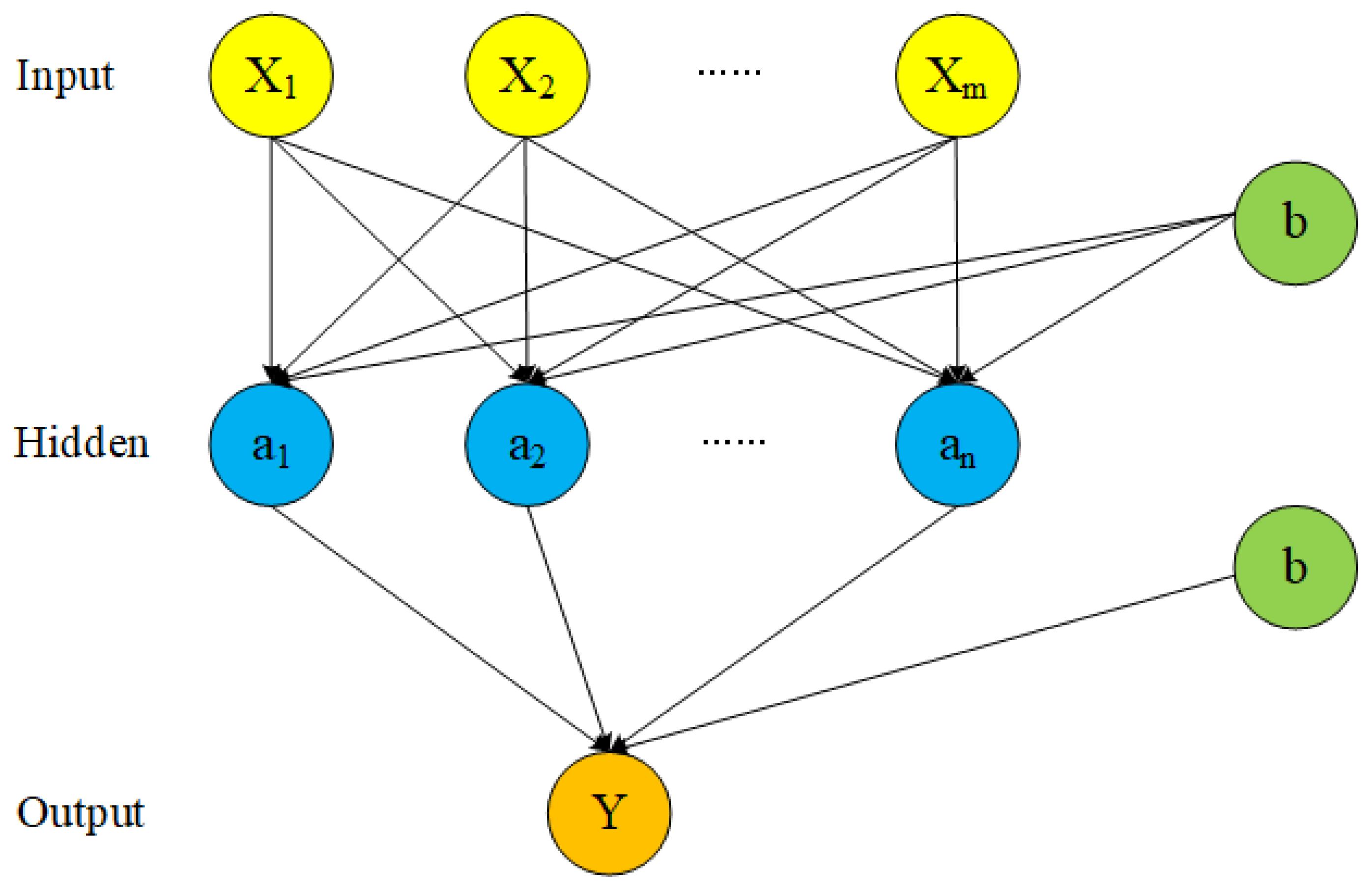
2.2.1. Backpropagation Neural Network

The backpropagation neural network (BPNN) is a multilayer neural network trained by an error backpropagation algorithm. The error after the output is used to estimate the error of the direct leading layer of the output layer, and then the error is used to estimate the error of the previous layer. If the reverse is passed down, the error estimates of all other layers are obtained [25]. This study used a feedforward three-layer BPNN with a mature algorithm. For details on the model algorithm, see Jin et al. [26]. A schematic of the network structure is shown in Figure 2.
The BPNN is chosen because it has the following advantages:
(1) Nonlinear mapping capability. A BPNN essentially realizes a mapping function from the input data to the output. Mathematical theories have proven that a three-layer neural network can approximate any nonlinear continuous function with arbitrary precision. This makes it particularly suitable for solving problems involving complex internal mechanisms.
(2) Self-learning and self-adaptive abilities. During training, the BPNN can automatically extract the “reasonable rules” between the input and output data through learning, and adaptively memorize the learning content in the weight of the network.
(3) Fault tolerance. The BPNN does not have a significant impact on the overall training results after its local or partial neurons are damaged, that is, the system can still work normally when it is locally damaged.

2.2.2. BPNN Optimized by Genetic Algorithm

Although the BPNN has some advantages, as stated above, it still has several shortcomings. For example, its algorithm is sensitive to the initialization weight matrix, and it easily falls into the local optimal solution; thus, the obtained solution is not the globally optimal solution. Therefore, researchers have proposed optimizing BPNN with intelligent algorithms [27], such as the particle swarm optimization algorithm and genetic algorithm (GA). After reviewing the literature, the present study applies the BPNN optimized by the GA.
The GA is an artificial intelligence optimization search algorithm that simulates biological evolution and natural selection in nature [28]. It has the characteristics of random search and global optimization, and is mainly used to solve optimization problems [29].

2.2.3. Multiple Linear Regression

Multiple linear regression models are used to investigate the relationship between dependent variables and multiple independent variables. They are usually used to describe the random linear relationship between variables as follows:
y = β 0 + β 1 x 1 + + β k x k + ζ ,
where x 1 x k are non-random variables, y is the dependent variable, β 0 β k are regression coefficients, and ξ is the random error term.

2.2.4. Support Vector Machine

The support vector machine (SVM) method is also a type of machine learning method that can be used to solve regression and classification problems. Here, we also introduce SVM to solve the problem of precipitation prediction in the YHRB. The basic principle is to find an optimal dividing line in a plane, in order to divide the data on the plane.
We used the built-in function newff of MATLAB 2016b for the BPNN, and the LIBSVM toolbox of MATLAB for the SVM method. The optimization algorithm comes from online forums with the improvement in this study.

2.3. Modeling Process

This study used data sets from 1979 to 2019. We used 33 (i.e., 1979–2011) and 8 (i.e., 2012–2019) years for the training and validation periods, respectively. In order to choose an appropriate method for summer precipitation forecasting, we compared several methods in which machine learning was dominant. Furthermore, to make the forecasts more accurate and obtain detailed information about the forecasts, we employed antecedent (i.e., winter and spring) factors for summer precipitation forecasts based on the information about single months; that is, a matrix of winter and spring months (i.e., six months) for factors and summer months (i.e., three months) for precipitation, constructed 18 schemes/models for monthly forecasts, and obtained the summer forecasts by summing up three monthly precipitation values.

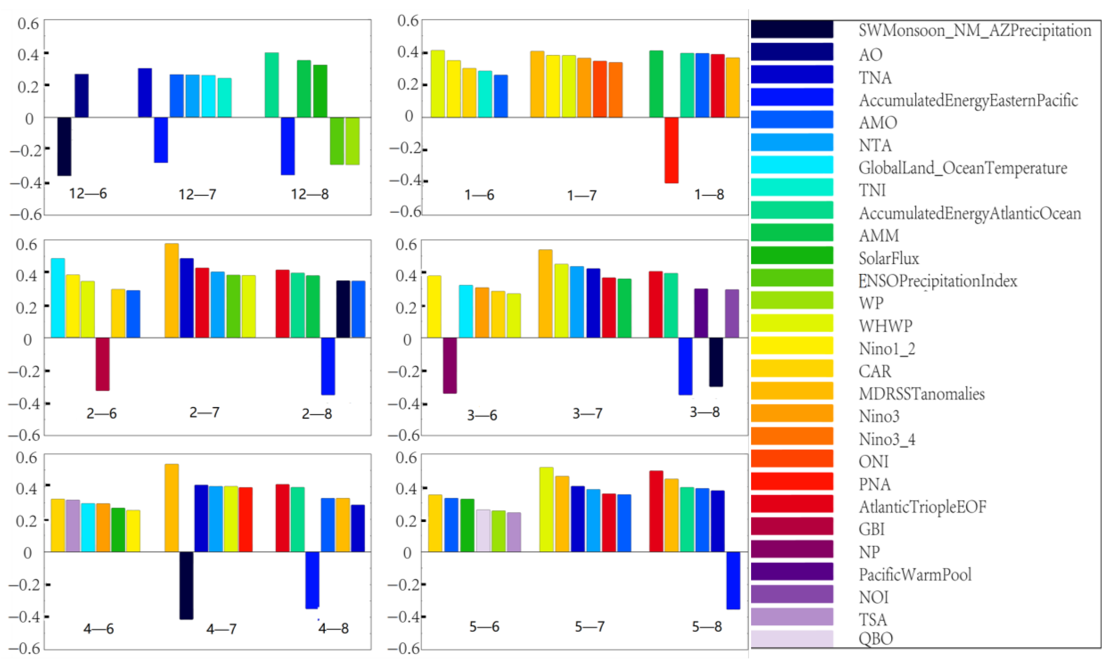
2.3.1. Factor Selection

As ANNs cannot automatically screen factors (i.e., predictors), a large number of factors will reduce the forecasting ability of the model. Therefore, prior to modeling, the factors must be screened in order to identify relatively more suitable variables for forecasts. Modeling uncertainties will certainly be an important aspect and will require concepts from Bayesian/probabilistic inference to be integrated, in order to directly address such uncertainties [30]. Factor selection can be performed using Pearson correlations between factors and precipitation, or principal component analysis (PCA) can be used to reduce the dimensionality of factors and form a set of new factors for forecasting [31]. This study aims to explore the relationship between the initial factors and summer precipitation in the YHRB; thus, the first method was used for factor screening. The absolute values of the obtained correlation coefficients were sorted from the largest to the smallest, and the confidence level was considered after calculating the correlation coefficients. Finally, the top six factors ranked by the absolute values of the correlation coefficients were selected from the factors that passed Student’s t-test at the 90% confidence level. Some models met the above conditions with fewer than six factors. Finally, the following factors were used to model the 18 schemes, as illustrated in Figure 3.
Figure 3 is the factor display diagram that is finally substituted into the model after the correlation analysis. In totality, 18 schemes correspond to 18 models. Each of the 18 models uses the factors of each of the previous 6 months (from December of the previous year to May of the current year) to predict the precipitation in a single month of June, July and August in the current summer.

2.3.2. Procedure of BPNN Forecasts

(a)
Standard BPNN modeling process
We employed standard BPNN for the summer precipitation forecast with the procedure as follows:
(i) Prescribing training and test periods. The precipitation and factor data for each of the 18 schemes were divided into training and test sets according to a certain ratio of time periods, and were used as the input and output of the BPNN, respectively, after normalized processing.
(ii) Determining the number of network input layers and hidden layer nodes. With regard to the hidden layer nodes, this study used Euler’s optimization algorithm. Considering the balance between computational resources and forecast precision, we selected six input layer factors for the seasonal precipitation forecast.
(iii) Performing network training. Weights and thresholds are constantly updated until the error requirements are met or until the prescribed maximum training times are reached.
(iv) Performing network testing, denormalizing the output values and completing precipitation prediction.
In modeling, the ratio of the length of the training set to the length of the test set is prescribed as 7:3 or 8:2 [32]. Considering the research sequence of the data used, the first 80% of the time series (from 1979 to 2011) was used as the training set, and the remaining 20% (from 2012 to 2019) of the data was used as the test set. Since this overall training set is subdivided into a training subset and a cross-validation subset when the built-in function of building a neural network is called in the process, there is no need to set part of the data for the cross-validation subset.
(b)
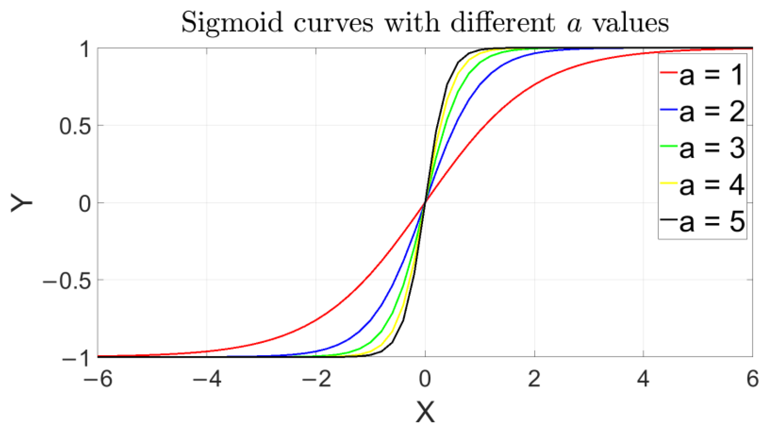
Activation function selection and parameter tuning
The widely used activation functions in ANNs include Sigmoid, Softmax, and ReLU. By considering the characteristics of the BPNN, this study uses the Sigmoid function (shown in Figure 4), with the horizontal and vertical axes corresponding to the value of the normalized data and calculated result, respectively, after introducing the function, which is expressed as follows:
f ( x ) = 1 / [ 1 + exp ( a x ) ]
Since the model selects the top six factors in the order of absolute values of the correlation coefficients, from the largest to the smallest, after the calculation of Pearson correlations and Student’s t-test at the 90% confidence level, with the final forecast as a variable of summer precipitation in the YHRB, the number of neurons in the input layer is the same as the number of input factors, and the number of neurons in the output layer is one.
The key parameter adjustment objective is the number of hidden layer nodes during the adjustment of the neural network parameters. Considering that the actual topography and climatic characteristics of each grid point of the calculated precipitation are different, this study builds different BP networks, one by one, for 342 grid points in the YHRB and adjusts the parameters of each network. For the number of hidden layer nodes, if the number of nodes is too small, the data features cannot be fully extracted; if the number of nodes is too large, the network complexity will increase and lead to overfitting. For the number of hidden layer nodes, the empirical formula is expressed as follows [33]:
m = n + l + b ,
where m and n are the number of hidden layer nodes and nodes in the input layer, respectively, and b is a constant in the range of 1–10.
Currently, most studies use a fixed value for the number of nodes in the middle layer within the range calculated according to empirical formulas [32]. In the ANN training process between grid points, the number of nodes in the middle layer is not necessarily the same. The present study used the Euler optimization algorithm to debug the parameter of the number of hidden layer nodes. The Euler optimization algorithm is a sub-function program developed in this study to determine the hidden layer nodes. The principle is based on the exhaustive method [33]. This algorithm takes the values of the hidden layer node range calculated by the empirical formula in turn, performs normalization and simulation, and calculates the mean square error of the training set and the mean square error (MSE) of each hidden layer. Finally, it finds the values of the hidden layer nodes corresponding to the minimum MSE, and uses the changed values as the number of hidden layer nodes of the grid points during modeling. According to the range of the parameter calculated using Equation (3), a cycle script was written in order to traverse the values within the range, and the value corresponding to the smallest calculated square error was used as the number of nodes in the hidden layer.

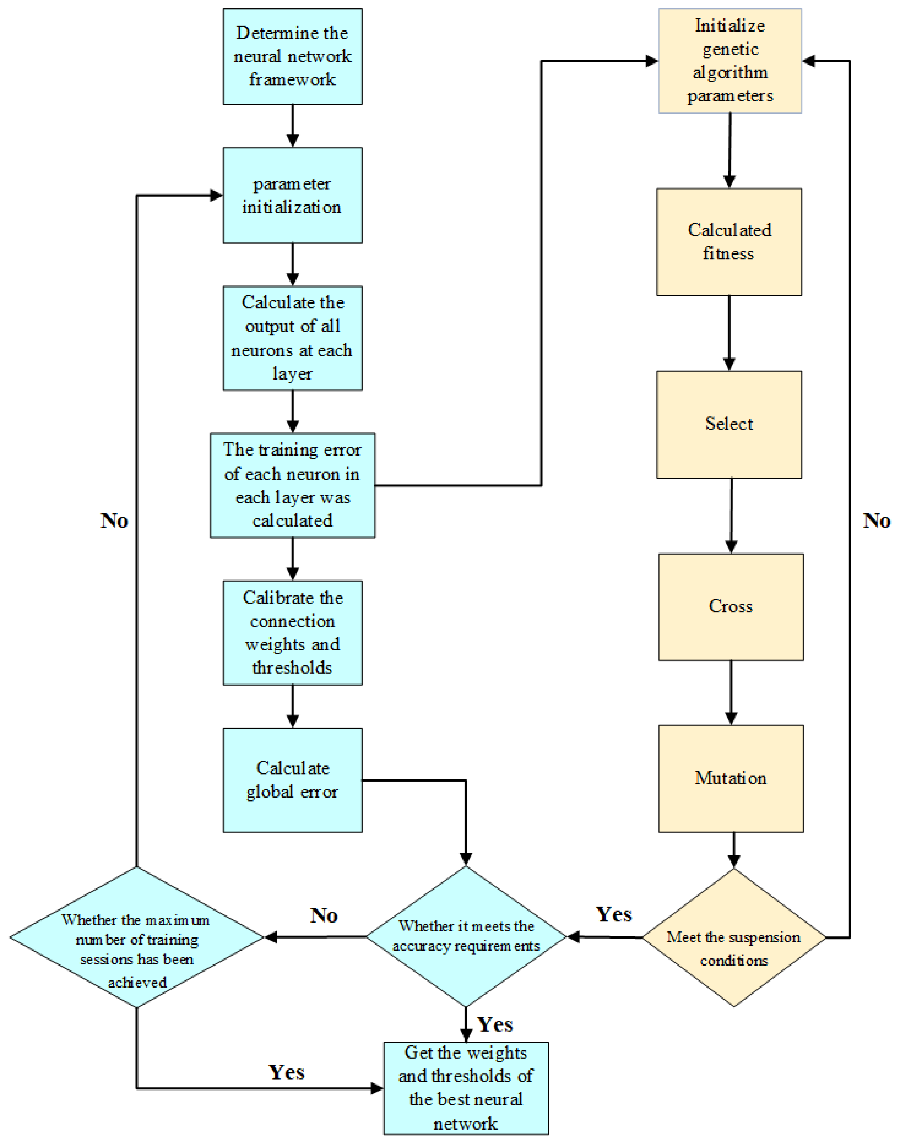
2.3.3. GABP Calculation Process

When a genetic algorithm is optimized, the relevant parameters are set. For example, the population number, crossover rate, mutation rate, and evolutionary generation number are prescribed as 50, 0.8, 0.1, and 100, respectively. A schematic of the calculation process is shown in Figure 5.

2.3.4. Multiple Linear Regression Calculation Process

The multiple linear regression method (MLR) is one of the most widely used traditional statistical methods, with a structure that is simple and easy to identify [34]. It assumes that there is a linear relationship between the forecasted quantity and predictors/factors. The conventional procedure is to use the training period data to calculate the unknown parameters, establish the forecast equation, and apply this equation to the forecast in the validation period. In this study, we established a linear regression model between multiple predictors and precipitation. Subsequently, correlation tests at the 0.95 confidence level were conducted.

2.4. Model Evaluation Measures

Three measures, that is, the average absolute error (MAE), mean absolute percentage error (MAPE) and root mean square error (RMSE), were used to evaluate and analyze the fitting and prediction accuracy of the models. They are calculated as follows:
MAE = 1 n ( i = 1 n | y i o i | )
RMSE = 1 n i = 1 n ( y i o i ) 2
MAPE = 1 n i = 1 n | y i o i y i | × 100 %
where o i is the observed precipitation, y i is the precipitation predicted by the model, and n is the grid number.
Additionally, previous studies [35,36,37] have used the anomaly rate (AR) to qualitatively evaluate the predicted precipitation and observations. The AR is based on whether the anomaly signs of the grid points in the forecast are consistent with those of the corresponding observations, which are evaluated over all of the stations (or grids) in the study domain [37]. The AR is computed using the following:
A R = n iden n × 100 %
where n iden is the number of the grids with identical signs of forecast and observed anomalies. Following previous studies [38], it is considered a good forecast when AR exceeds 50%.

3. Predicted Results

3.1. Comparison of Basin-Averaged Measures among the Four Methods

Figure 6 shows the overall basin-averaged statistical measures of precipitation predicted by the four methods, with the variability of each method included. It can be concluded that the prediction accuracies of BPNN and MLR are comparable, but the stability of BPNN is stronger than that of MLR; that is, MLR has higher variability. In addition, the SVM produces better forecasts than the BPNN and MLR, while the GABP outperforms the BPNN, SVM and MLR; for example, the BPNN yields overall MAPE, MAE and RMSE values of approximately 87%, 115 mm and 138 mm, respectively, for the YHRB, whereas GABP yields significantly reduced values of 20%, 27 mm and 35 mm, respectively.
Table 1 lists specific values of the month (predictor)-to-month (forecast) results of the measures. It can be noted that the GABP gives better predictions than the BPNN, SVM and MLR for monthly precipitation in summer, which is consistent with the above-mentioned results. For example, the GABP presents MAPE values of approximately 20–50%, corresponding to the SVM, BPNN and MLR values of 30–62%, 70–110% and 46–215%, respectively, showing the order of a worsening performance. Additionally, the GABP accuracies of the summer precipitation forecast models established by the previous winter factors are higher than those by the spring factors. For example, using the December factors, GABP presents region-averaged MAPE values of 19.7%, 27.4% and 15.9% for June, July and August, respectively, which are lower than those by March, April or May factors.

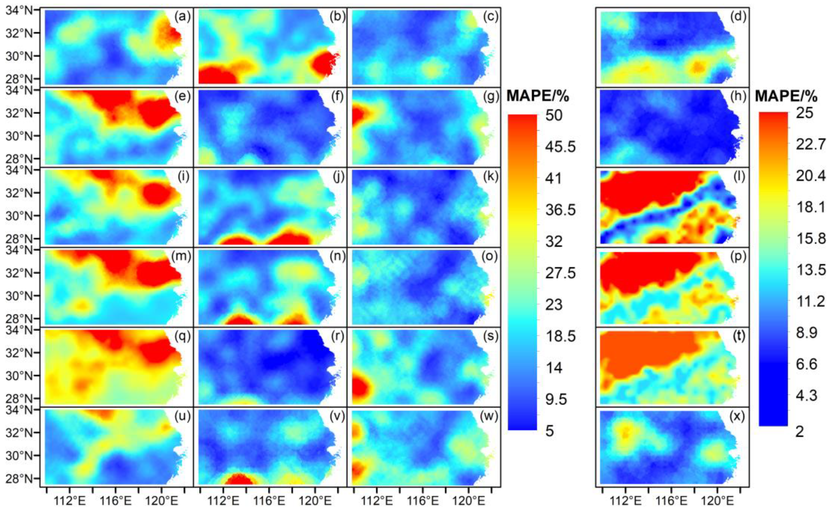
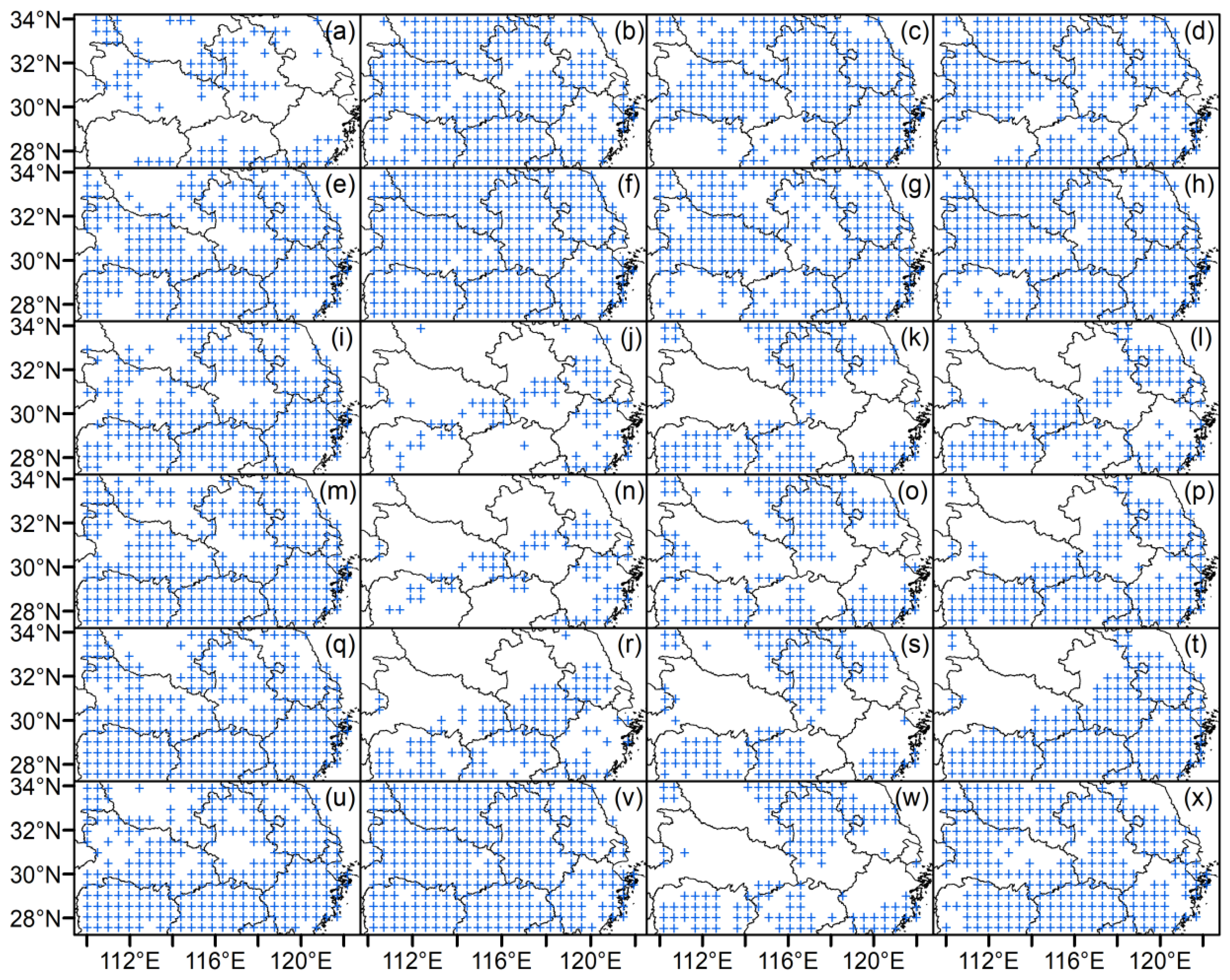
3.2. GABP-Produced Spatial Distributions of the Measures

Because the above results indicate that GABP is the best among the methods, this subsection presents the distributions of evaluation measures of MAPE and AR using GABP only.
Figure 7 shows the spatial distributions of MAPE, indicating that the MAPE values decrease in the order of June, July and August, with large total areas of values lower than 20% and small areas of values larger than 50%. In addition, large MAPE values were observed over the northern YHRB. However, the accumulated summer precipitation showed reduced MAPE values, which were lower than 30%. It appears that the model with January factors had the lowest overall MAPE values (as low as less than 10%) among the models with factors of different winter or spring months.
It can be observed from Figure 8 and Table 1 that most of the basin-averaged AR values of 18 GABP models for single months exceed 50%, which indicates the reliability of the precipitation forecasts. The summer AR (i.e., the right column in Figure 8) shows good performance of GABP forecasts, except for the model using February factors (Figure 8l), whereas the model using January factors is the best with an AR of 88.3% (Figure 8h; Table 2). Furthermore, there is a correlation between MAPE and AR; that is, smaller MAPE values correspond to larger AR values (e.g., for summer forecasts in the right columns of MAPE and AR; Figure 7d,h,l,p,s,t,v,x; Figure 8d,h,l,p,t,x).

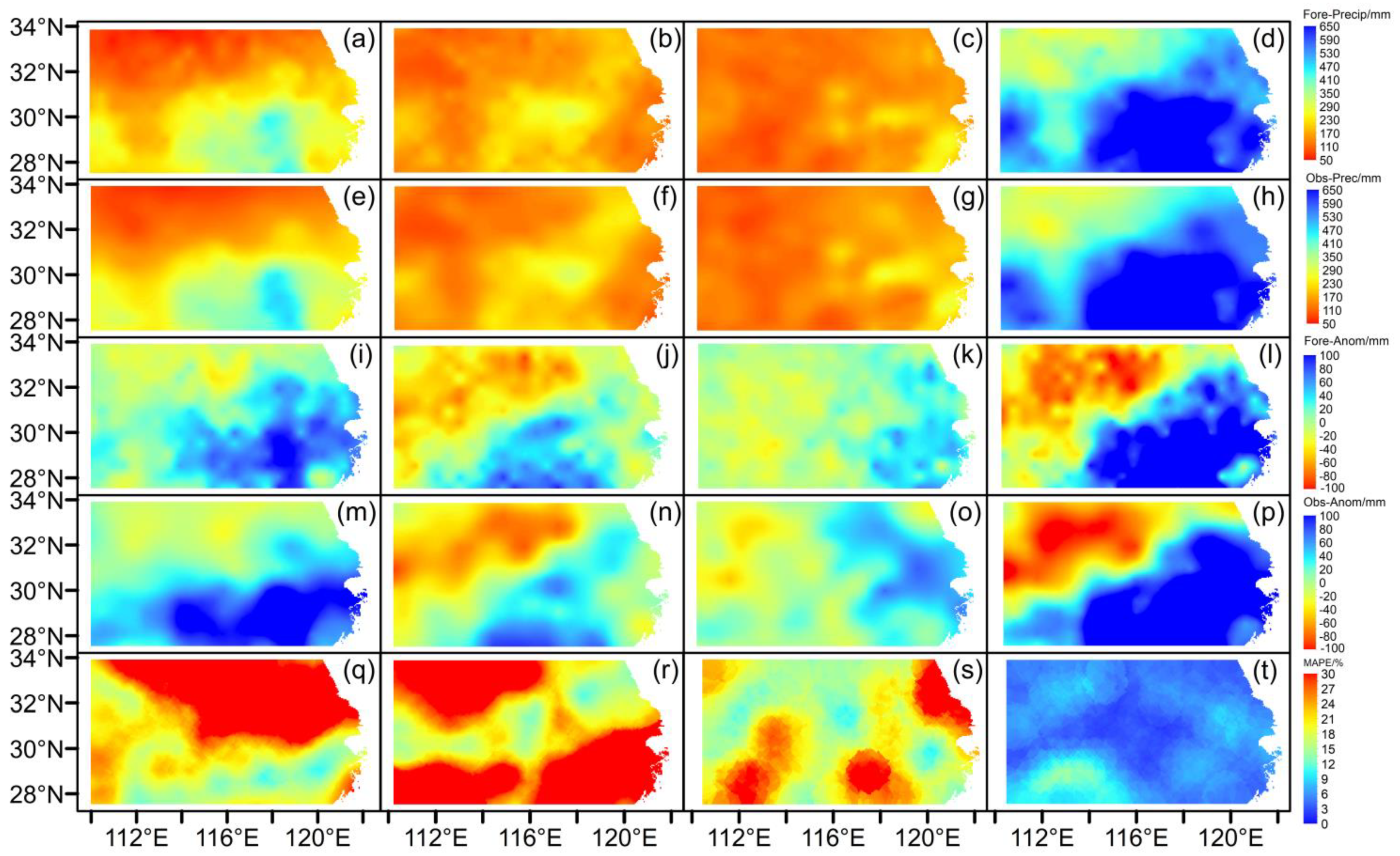
3.3. Spatial Distributions of Forecasted Summer Precipitation by the Best GABP Model

It is noteworthy that the prediction plots versus observed values can provide useful information for the training and validation periods. However, because there are a large amount of results in this study, we only present some of them. For example, we have 18 month (predictors)-to-month (precipitation) models for each of the BPNN, GABP, SVM and MLR methods, which make it inappropriate to present the plots of all models of the specific training and validation periods. Please see Supplementary Information for more details of the BPNN, GABP, SVM and MLR precipitations and an example using March factors in the training and validation periods (Figures S1–S8; Table S1), which indicates that there is no significant underfitting or overfitting for monthly precipitations in this study.
The above-mentioned results indicate that GABP is the best method, in which the model using January factors is the best among the models with different monthly factors. Therefore, for the sake of concise presentation we can choose the GABP model with January factors as the “best” forecast model for future operational services.
Figure 9 shows the spatial distributions of the “best” GABP precipitation forecast averaged over the test period of 2012–2019. It can be noted that the GABP model using January factors successfully produces the precipitation forecast both in absolute values and anomalies; for example, forecasted summer precipitation in the YHRB gradually decreased from southeast to northwest, and higher-than-normal precipitation occurred in the southeastern YHRB, which is consistent with observations. In addition, the MAPE values were generally lower than 10%, corresponding to a very low basin-averaged value of 4.7% (Table 1).

4. Concluding Remarks

In this study, we used an ANN for summer precipitation forecasts in the YHRB. Using NOAA CPC analysis of precipitation and the previous large-scale predictors/factors and sea surface temperatures that are openly available via Internet resources, we calculated the correlation coefficients between the precipitation and the factors. In addition, we sorted the top six factors for precipitation forecast according to the principle of the significant correlations at the 90% confidence level. Then, the month (factors)-to-month (precipitation) models were trained and tested over 33 (i.e., 1979–2011) and 8 (i.e., 2012–2019) years of summer months for the training and validation periods, respectively. These models employed the BPNN, GABP (i.e., BPNN with a genetic algorithm) and MLR methods, whose results of forecasted precipitation for the summer months were compared. The major conclusions are as follows:
(1) The GABP method was the best among the above methods for precipitation forecasting. While the BPNN model had a strong nonlinear mapping ability and performed slightly better than the traditional MLR models with less variability, the GABP models had much higher precision than the standard BPNN models in terms of the MAE, MAPE, RMSE and AR measures. For example, the BPNN yielded basin-averaged MAPE, MAE and RMSE values of approximately 87%, 115 mm and 138 mm, respectively, whereas the GABP errors were significantly reduced with corresponding values of approximately 20%, 27 mm and 35 mm, respectively.
(2) By comparing the month-to-month forecasts, the best forecast was found to be produced by the GABP model using January factors by summing up the forecasted June, July and August precipitation, which is suggested as a recommendation for future operational service. This GABP model has a basin-averaged MAPE of 4.7% and an AR of 88.3%, making it a substantially more successful tool than the current operational service [39].
(3) There are many uncertainties in the model building process, including the selection of the type and number of predictors in the early stage, determination of the number of network layers and nodes in the neural network, and optimization of parameters. For practical applications of machine learning, it is recommended that the differences between different models and predictors be compared. In this case, we used the month (factors)-to-month (precipitation) mode, and obtained the best GABP model using the January factors for individual summer months. Since these January factors are currently openly available with regularly updated values, the GABP forecast is practical in the operational service. Furthermore, some specific algorithms should be elaborated for the ANN forecasts. For example, the Euler optimization algorithm used in this study calculates the error to adjust the number of neurons in the hidden layer in order to fix a certain value, which is effective in the GABP forecast.
In this study, according to the factor selection criteria, 28 of the 42 factors provided by the websites are used, and they appear 103 times in total in our 18 month-to-month models. More than half of the 28 factors are SST factors, and the total frequency of these SST factors is 52 out of 103 times. This clearly shows the importance of SST factors in summer precipitation prediction in the YHRB, which is consistent with previous studies that emphasized the importance of SST [19]. The YHRB is located in the East Asian monsoon zone [40], featuring low terrain and high vegetation coverage in the semi-humid and humid climates [41] where summer precipitation is highly affected by SSTs over some key areas. The issue that the SSTs highly influence seasonal precipitation forecasts has been found for various regions worldwide [42,43]. For example, the statistical forecasts were achieved using a correlation coefficient up to 0.75 and the lowest mean relative error of 6% by establishing a linear regression relationship between the SST and rainfall for the Yangtze River basin [43]. The reason that the SSTs substantially affect the East Asia precipitation is as follows: The atmospheric thermal state over the oceans can be influenced by the SSTs, which induce convective activities and further cause the change in atmospheric circulation regionally and then globally with the propagation of atmospheric waves [44,45,46]. With the SST-induced circulation changes in the YHRB, the precipitation is subsequently changed. It appears that the SST factors such as Main Development Region (MDR) SST anomalies, Niño 1_2 SST, Oceanic Niño Index (ONI), and Western Hemisphere Warm Pool (WHWP) SST play important roles in the forecasts of this study (Figure 3).
It should be noted that in terms of dynamical forecasting, useful dynamical information provided by general circulation models (GCM) can contribute to seasonal forecasts. However, due to the deficiencies of GCM in model frameworks and numerical computation, large errors might still be induced, probably resulting in a phenomena of climate drifting. In reviewing the forecast precision of this study, it appears that the statistical method of machine learning using antecedent predictors can serve as an effective method for summer precipitation forecasts.

Supplementary Materials

The following supporting information can be downloaded at: https://www.mdpi.com/article/10.3390/atmos13060929/s1. Figure S1: Spatial distributions of MAPE of SVM forecasts, where the six rows are for models using the factors of December, January, February, March, April and May (from top to bottom), with four columns for the forecasted precipitations of June, July, August and summer (from left to right), respectively. Figure S2: Spatial distribution of identical signs of SVM forecast precipitation anomalies, where six rows and four columns are the same as those in Figure 7 for various months of factors and months/season of precipitation forecast, respectively, and the grids with identical signs of forecast and observed anomalies are marked with crosses (i.e., “+”), through which the AR is calculated. Figure S3: As Figure S1, but for GABP MAPE in the training period. Figure S4: As Figure S3, but for observed mean precipitations in the training (upper) and validation (lower) periods (units: mm). Figure S5: As Figure S4, but for BPNN precipitations using March factors in the training (upper) and validation periods. Figure S6: As Figure S5, but for GABP precipitations. Figure S7: As Figure S5, but for SVM precipitations. Figure S8: As Figure S5, but for MLR precipitations. Table S1: The GABP basin-averaged MAPE values in the training period.

Author Contributions

Conceptualization, X.-M.Z.; methodology, Z.-C.Z., X.-M.Z. and B.-Z.W.; software, Z.-C.Z. and B.-Z.W.; validation, Z.-C.Z., X.-M.Z. and B.-Z.W.; formal analysis, Z.-C.Z., X.-M.Z. and B.-Z.W.; investigation, Z.-C.Z., X.-M.Z. and G.L.; resources, Z.-C.Z., X.-M.Z., G.L. and B.L.; data curation, Z.-C.Z., X.-M.Z., G.L., B.L. and M.-Z.X.; writing—original draft preparation, Z.-C.Z. and X.-M.Z.; supervision, X.-M.Z.; project administration, X.-M.Z.; funding acquisition, X.-M.Z., B.L. and M.-Z.X. All authors have read and agreed to the published version of the manuscript.

Funding

This research was financially supported by the National Key Research and Development Program of China (Grant Nos. 2021YFA070298 and 2021YFA0718000) and the National Natural Science Foundation of China (Grant Nos. U2240248, 51909057 and 41775087).

Institutional Review Board Statement

Not applicable.

Informed Consent Statement

Not applicable.

Data Availability Statement

The data in this study can be available, as listed in Appendix A.

Conflicts of Interest

The authors declare no conflict of interest.

Appendix A. Predictors/Indices Used for Precipitation Forecast with Available Resources Listed

SOISouthern Oscillation Index; NOAA Climate Prediction Center (CPC)
PNAPacific North America Index; NOAA Climate Prediction Center (CPC)
NAONorth Atlantic Oscillation Index; NOAA Climate Prediction Center (CPC)
ONIOcean Nino Index; NOAA Climate Prediction Center (CPC)
NTATropical North Atlantic Sea Temperature Index; ERSST V3b data set
CARCaribbean Sea Temperature Index; NOAA ERSST V3b data set
ENSO precipitation indexENSO precipitation index; http://precip.gsfc.nasa.gov/ESPItable.html, accessed on 6 June 2021
BESTBivariate ENSO time series; NOAA OI V2 SST data set
Nino3Tropical East Pacific Sea Temperature; NOAA ERSST V5 data set
Nino4Tropical Central Pacific Sea Temperature; NOAA ERSST V5 data set
Nino1+2Extreme eastern tropical Pacific sea temperature; NOAA ERSST V5 data set
Nino3+4The sea temperature of the tropical central and eastern Pacific Ocean; NOAA ERSST V5
TNATropical North Atlantic Index; HadISST and NOAA OI 1° × 1° data set
TSATropical South Atlantic Index, from HadISST and NOAA OI 1° × 1° data set
Atlantic Tripole SST EOFThe first EOF mode of the tropical Atlantic SST
WPWestern Pacific Index; NOAA Climate Prediction Center (CPC)
QBOQuasi-Biennial oscillation; zonal average of the equatorial 30mb zonal wind calculated by NCEP/NCAR reanalysis
WHWPMonthly anomaly of the western hemisphere warm pool area above 28.5 degrees; HadISST and NOAA OI datasets
PDOPacific Interdecadal Oscillation; NOAA Climate Prediction Center (CPC)
NOIArctic Oscillation Index; NOAA Climate Prediction Center (CPC)
NPNorth Pacific Oscillation; NOAA Climate Prediction Center (CPC)
EPEast Pacific Oscillation; NOAA Climate Prediction Center (CPC)
AAOAntarctic Oscillation; NOAA Climate Prediction Center (CPC)
Pacific Warmpool SST EOFfirst mode of Pacific Warmpool; NOAA OI 1° × 1° data set
Tropical Pacific SST EOFTropical Pacific SST EOF first mode; NOAA OI 1° × 1° data set
TNIEl-Niño Evolution Index; http://psl.noaa.gov/Pressure/Timeseries/TNI/, accessed on 6 June 2021
AMOAtlantic Multidecadal Oscillation long version; Kalplan sea surface temperature
AMMAtlantic meridian model; NOAA Climate Prediction Center (CPC)
IndianRainfall Index in Central India; http://www.tropmet.res.in/, accessed on 6 June 2021
SahelSahel regional precipitation index; http://jisao.washington.edu/data_sets/sahel/Mitchell, accessed on 6 June 2021
NAONorth Atlantic Oscillation; University of East Anglia Climatic Research Unit (CRU)
MEIMultivariate ENSO Index; NOAA PSL data
AOArctic Oscillation; NOAA Climate Prediction Center (CPC)
BrazilPrecipitation anomalies in northeastern Brazil; http://jisao.washington.edu/data_sets/brazil/, accessed on 6 June 2021
Solar Fluxfrom ftp://ftp.ngdc.noaa.gov/STP/space-weather/solar-data/, accessed on 6 June 2021
Hurricane activityMonthly Atlantic hurricanes and tropical storms; Colorado State University
Global Mean Land/Ocean TemperatureNASA Goddard Institute for Space Studies (GISS)
SW Monsoon Region rainfallAverage rainfall in Arizona and New Mexico; the climate department of NCDC
MDRSSTMDR minus tropical sea temperature observation anomalies, PSL from NOAA
AEEPAccumulated Energy Eastern Pacific; NOAA Climate Prediction Center (CPC)
AEAOAccumulated Energy Atlantic Ocean; NOAA Climate Prediction Center (CPC)
Atlantic Tripole EOFThe first EOF mode of tropical Pacific SST; NOAA Climate Prediction Center (CPC)

References

  1. Wu, J.D.; Fu, Y.; Zhang, J.; Li, N. Analysis on the trend of meteorological disasters in China from 1949 to 2013. J. Nat. Resour. 2014, 29, 1520–1530. (In Chinese) [Google Scholar]
  2. Liu, Y.Y.; Ding, Y.H. Characteristics and possible causes for extreme Meiyu in 2020. Meteor. Mon. 2020, 46, 1483–1493. (In Chinese) [Google Scholar]
  3. Peng, Y.Z.; Wang, Q.; Yuan, C.; Lin, K.P. Review of Research on Data Mining in Application of Meteorological Forecasting. J. Arid Meteorol. 2015, 33, 19–27. (In Chinese) [Google Scholar]
  4. Li, C.Y. Climate Dynamics, 2nd ed.; Chapter 1; Meteorological Press: Beijing, China, 2000; pp. 2–3. [Google Scholar]
  5. Wang, X.; Song, L.C.; Wang, G.F.; Ren, H.L.; Wu, T.W.; Jia, X.L.; Wu, H.P.; Wu, J. Operational climate prediction in the era of big data in China: Reviews and prospects. J. Meteorol. Res. 2016, 30, 444–456. [Google Scholar] [CrossRef]
  6. Arcomano, T.; Szunyogh, I.; Pathak, J.; Wikner, A.; Hunt, B.R.; Ott, E. A machine learning-based global atmospheric forecast model. Geophys. Res. Lett. 2020, 47, e2020GL087776. [Google Scholar] [CrossRef]
  7. Bauer, P.; Thorpe, A.; Brunet, G. The quiet revolution of numerical weather prediction. Nature 2015, 525, 47–55. [Google Scholar] [CrossRef] [PubMed]
  8. Reichstein, M.; Camps-Valls, G.; Stevens, B.; Jung, M.; Denzler, J.; Carvalhais, N.; Prabhat. Deep learning and process understanding for data-driven Earth system science. Nature 2019, 566, 195–204. [Google Scholar] [CrossRef]
  9. Gómez-Chova, L.; Tuia, D.; Moser, G.; Camps-Valls, G. Multimodal classification of remote sensing images: A review and future directions. Proc. IEEE 2015, 103, 1560–1584. [Google Scholar] [CrossRef]
  10. Camps-Valls, G.; Tuia, D.; Bruzzone, L.; Benediktsson, J.A. Advances in hyperspectral image classification: Earth monitoring with statistical learning methods. IEEE Signal. Process. Mag. 2014, 31, 45–54. [Google Scholar] [CrossRef] [Green Version]
  11. Gislason, P.O.; Benediktsson, J.A.; Sveinsson, J.R. Random forests for land cover classification. Pattern Recogn. Lett. 2006, 27, 294–300. [Google Scholar] [CrossRef]
  12. Muhlbauer, A.; McCoy, I.L.; Wood, R. Climatology of stratocumulus cloud morphologies: Microphysical properties and radiative effects. Atmos. Chem. Phys. 2014, 14, 6695–6716. [Google Scholar] [CrossRef] [Green Version]
  13. Pan, B.; Hsu, K.; AghaKouchak, A.; Sorooshian, S. Improving precipitation estimation using convolutional neural network. Water Resour. Res. 2019, 55, 2301–2321. [Google Scholar] [CrossRef] [Green Version]
  14. Toms, B.A.; Barnes, E.A.; Ebert-Uphoff, I. Physically interpretable neural networks for the geosciences: Applications to Earth system variability. J. Adv. Modeling Earth Syst. 2020, 12, e2019MS002002. [Google Scholar] [CrossRef]
  15. Sharifi, E.; Saghafian, B.; Steinacker, R. Downscaling satellite precipitation estimates with multiple linear regression, artificial neural networks, and spline interpolation techniques. J. Geophys. Res. Atmos. 2019, 124, 789–805. [Google Scholar] [CrossRef] [Green Version]
  16. Nearing, G.S.; Kratzert, F.; Sampson, A.K.; Pelissier, C.S.; Klotz, D.; Frame, J.M.; Prieto, C.; Gupta, H.V. What role does hydrological science play in the age of machine learning? Water Resour. Res. 2021, 57, e2020WR028091. [Google Scholar] [CrossRef]
  17. Pham, Q.; Yang, T.-C.; Kuo, C.-M.; Tseng, H.-W.; Yu, P.-S. Combing Random Forest and Least Square Support Vector Regression for Improving Extreme Rainfall Downscaling. Water 2019, 11, 451. [Google Scholar] [CrossRef] [Green Version]
  18. Kang, J.; Wang, H.; Yuan, F.; Wang, Z.; Huang, J.; Qiu, T. Prediction of summer precipitation in China based on LSTM network. Clim. Change Res. 2020, 16, 263–275. [Google Scholar]
  19. He, C.; Wei, J.; Song, Y.; Luo, J.-J. Seasonal Prediction of Summer Precipitation in the Middle and Lower Reaches of the Yangtze River Valley: Comparison of Machine Learning and Climate Model Predictions. Water 2021, 13, 3294. [Google Scholar] [CrossRef]
  20. Gagne, D.J., II; McGovern, A.; Xue, M. Machine Learning Enhancement of Storm-Scale Ensemble Probabilistic Quantitative Precipitation Forecasts. Weather. Forecast. 2014, 29, 1024–1043. [Google Scholar] [CrossRef] [Green Version]
  21. Zhang, F.; Wang, X.; Guan, J. A Novel Multiple-Input Multiple-Output Recurrent Neural Network Based on Multimodal Fusion and Spatiotemporal Prediction for 0–4 h Precipitation Nowcasting. Atmosphere 2021, 12, 1596. [Google Scholar] [CrossRef]
  22. Kishtawal, C.M.; Basu, S.; Patadia, F.; Thapliyal, P.K. Forecasting summer rainfall over India using genetic algorithm. Geophys. Res. Lett. 2003, 30, 2203. [Google Scholar] [CrossRef]
  23. Feng, Y.; Zhang, W.F.; Sun, D.Z.; Zhang, L.Q. Ozone concentration forecast method based on genetic algorithm optimized back propagation neural networks and support vector machine data classification. Atmos. Environ. 2011, 45, 1979–1985. [Google Scholar] [CrossRef]
  24. Huang, X.Y.; Zhao, H.S.; Huang, Y.; Lin, K.P.; He, L. Application of genetic-neural network ensemble forecasting method to tropical cyclone precipitation forecast in Guangxi. J. Nat. Disasters 2017, 26, 184–196. [Google Scholar]
  25. Jin, L. Theory and Application of Neural Network Weather Forecast Modeling; China Meteorological Press: Beijing, China; pp. 41–45. (In Chinese)
  26. Jin, L.; Luo, Y.; Li, Y.H. Study on mixed prediction model of artificial neural for long range weather. J. Syst. Engi. 2003, 18, 331–336. (In Chinese) [Google Scholar]
  27. Zhao, J.L. Genetic algorithm for solving nonlinear optimization problems. Prog. Geophys. 1992, 7, 90–97. (In Chinese) [Google Scholar]
  28. Peng, Z.L. Research on China’s Seasonal Precipitation Forecast and Application Based on the Combination of Statistical Model and Dynamic Multi-Model; Dalian University of Technology: Dalian, China, 2014. (In Chinese) [Google Scholar]
  29. Wang, J.Z.; Liu, L.; Xu, J.Y. Daily flow forecast based on genetic algorithm and support vector machine. Hydropower Energy Sci. 2008, 26, 14–17. (In Chinese) [Google Scholar]
  30. Ghahramani, Z. Probabilistic machine learning and artificial intelligence. Nature 2015, 521, 452–459. [Google Scholar] [CrossRef]
  31. Liu, X.P.; Wang, H.J.; He, M.Y. Estimation of precipitation under future climate scenarios in the Yangtze-Huaihe region statistical downscaling. Adv. Water Sci. 2012, 23, 29–37. (In Chinese) [Google Scholar]
  32. Du, Y.; Long, K.H.; Wang, D.Y.; Wang, D.G. Prediction of annual precipitation in Anhui Province based on machine learning methods. Hydropower Energy Sci. 2020, 38, 5–7. (In Chinese) [Google Scholar]
  33. Sun, Y.X.; Feng, N. Application of Exhaustive Method in Programming. Comput. Times 2012, 8, 50–52. [Google Scholar]
  34. Shen, H.Y.; Wang, Z.X.; Qin, J. Determining the number of BP neural network hidden layer units. J. Tianjin Univ. Technol. 2008, 5, 13–15. (In Chinese) [Google Scholar]
  35. Zhen, Y.W.; Hao, M.; Lu, B.H.; Zuo, J.; Liu, H. Research of Medium and Long Term Precipitation Forecasting Model Based on Random Forest. Water Resour. Power 2015, 6, 6–10. [Google Scholar]
  36. Bai, H.; Gao, H.; Liu, C.Z. Assessment of Multi-model Downscaling Ensemble Prediction System for Monthly Temperature and Precipitation Prediction in Guizhou. J. Desert Oasis Meteorol. 2016, 10, 58–63. (In Chinese) [Google Scholar]
  37. Yao, S.B.; Jiang, D.B.; Fan, G.Z. Projection of precipitation seasonality over China. Chin. J. Atmos. Sci. 2018, 42, 1378–1392. (In Chinese) [Google Scholar]
  38. Yang, Y.; Dai, X.G.; Tang, H.W.; Zhang, B. CMIP5 Model Precipitation Bias-correction Methods and Projected China Precipitation for the Next 30 Years. Clim. Environ. Res. 2019, 24, 769–784. (In Chinese) [Google Scholar]
  39. Wang, H.; Ren, H.; Chen, H.; Jiehua, M.; Baoqiang, T.; Bo, S.; Yanyan, H.; Mingkeng, D.; Jun, W.; Lin, W. Highlights of climate prediction study and operation in China over the past decades. Acta Meteorol. Sin. 2020, 78, 317–331. (In Chinese) [Google Scholar]
  40. Ding, Y.; Chan, J.C.L. The East Asian summer monsoon: An overview. Meteor. Atmos. Phys. 2005, 89, 117–142. [Google Scholar]
  41. Zeng, X.M.; Wang, M.; Wang, N.; Yi, X.; Chen, C.H.; Zhou, Z.G.; Wang, G.L.; Zheng, Y.Q. Assessing simulated summer 10-m wind speed over China: Influencing processes and sensitivities to land surface schemes. Clim. Dyn. 2018, 50, 4189–4209. [Google Scholar] [CrossRef]
  42. Chen, C.; Georgakakos, A.P. Hydro-climatic forecasting using sea surface temperatures: Methodology and application for the southeast US. Clim. Dyn 2014, 42, 2955–2982. [Google Scholar] [CrossRef]
  43. Qian, S.N.; Chen, J.; Li, X.Q.; Xu, C.Y.; Guo, S.L.; Chen, H.; Wu, X.S. Seasonal rainfall forecasting for the Yangtze River basin using statistical and dynamical models. Int. J. Climatol. 2020, 40, 361–377. [Google Scholar] [CrossRef]
  44. Nitta, T. Convective activities in the tropical western Pacific and their impact on the Northern Hemisphere summer circulation. J. Meteor. Soc. Jpn. 1987, 64, 373–390. [Google Scholar] [CrossRef] [Green Version]
  45. Zhang, R.; Sumi, A.; Kimoto, M. Impact of El Niño on the East Asian monsoon. J. Meteor. Soc. Jpn. 1996, 74, 49–62. [Google Scholar] [CrossRef] [Green Version]
  46. Huang, R.; Gu, L.; Zhou, L.; Shangsen, L. Impact of the thermal state of the tropical western Pacific on onset date and process of the South China Sea summer monsoon. Adv. Atmos. Sci. 2006, 23, 909–924. [Google Scholar] [CrossRef]
Figure 1. Study area of the YHRB denoted by the land portion in the red box.
Atmosphere 13 00929 g001
Figure 2. Schematic diagram of the three-layer BPNN structure, where X and Y are the input and output layer variables, respectively. The input and output layers are connected, separately, by the neuron with the hidden layer as the node.
Atmosphere 13 00929 g002
Figure 3. Correlation coefficient between a factor of an antecedent month in the previous winter/spring and the precipitation of a month in summer (e.g., “12-6” means the correlation between a December factor and the following June precipitation).
Atmosphere 13 00929 g003
Figure 4. Sigmoid activation function used in the BPNN, where a is taken as 1 for practice in this study (i.e., shown in the red line).
Atmosphere 13 00929 g004
Figure 5. Schematic diagram of the calculation process, in which the blue part represents the standard BPNN, while the yellow part illustrates the optimization process based on the standard BPNN using the genetic algorithm.
Atmosphere 13 00929 g005
Figure 6. Box diagrams of the maximum, minimum and average errors of predicted summer precipitation using the four methods for the YHRB, where (ac) are for MAPE, MAE and RMSE, respectively.
Atmosphere 13 00929 g006
Figure 7. Spatial distributions of MAPE by GABP, where the six rows are for models using the factors of December, January, February, March, April and May (from top to bottom; e.g., (ad) are for December factors), with four columns for the forecasted precipitations of June, July, August and summer (from left to right; e.g., (b,f,j,n,r,v) are for July precipitations), respectively.
Atmosphere 13 00929 g007
Figure 8. Spatial distribution of identical signs of GABP forecast precipitation anomalies, where rows and columns are the same as those in Figure 7 for various months of factors and months/season of precipitation forecast (e.g., (eh) are for January factors, and (mp) are for identical signs of precipitations of June, July, August and summer, respectively), respectively, and the grids with identical signs of forecast and observed anomalies are marked with crosses (i.e., “+”), through which the AR is calculated.
Atmosphere 13 00929 g008
Figure 9. Spatial distributions of the “best” summer precipitation forecasts using January factors by GABP over the test periods [i.e., eight-month (summer) means over 2012–2019], where the first and second rows indicate forecasted precipitations with absolute values and corresponding observations, respectively (e.g., (ad) are for forecasted June, July, August and summer precipitations, respectively, with (eh) corresponding to the observations, respectively); the third and fourth rows are the same as the first and second rows, respectively, but for anomalies; the fifth row represents MAPE distributions; the columns from left to right show results for June, July, August and summer, respectively.
Atmosphere 13 00929 g009
Table 1. Basin-averaged evaluation measures of various models, where each model is denoted with a subscript that contains two numbers; the former and latter numbers are respectively for the month of factors selected and the month of forecasted precipitation; e.g., M12-6 means the model using the December factors to predict the June precipitation (also shown are the values in brackets in correspondence with the model in brackets).
MeasureMethodM12-6M12-7M12-8M1-6M1-7M1-8M2-6M2-7M2-8
(M3-6)(M3-7)(M3-8)(M4-6)(M4-7)(M4-8)(M5-6)(M5-7)(M5-8)
MAPE/%BPNN108.394.173.484.657.794.379.79489
(98.1)(86.6)(92.7)(80.7)(62.7)(88.8)(71.7)(78.6)(109.5)
GABP19.727.415.929.613.918.823.821.316
(31.5)(19.9)(17.1)(27.6)(12.9)(20.4)(31.3)(18.3)(20.6)
SVM43.858.632.351.361.93951.545.441.5
(52.8)(45.6)(43.1)(52)(33.5)(44.3)(46.5)(61.5)(44.9)
MLR51.976.669.571.245.757.563.572121
(98.6)(160.1)(87.7)(60)(171.8)(63.9)(81.3)(79.9)(214.3)
MAE/mmBPNN130.3115.7100.4122.4112.7108.2107.7132.2109.7
(136.3)(127.9)(106.2)(123.9)(112.4)(107.4)(104.4)(116.8)(121.7)
GABP2531.620.238.623.321.431.829.418.8
(42.5)(29.7)(18.8)(41.2)(21.8)(24.1)(32.9)(26.8)(23.8)
SVM50.465.446.271.761.243.565.468.149.2
(80.4)(66.3)(47.4)(78.3)(60)(52.8)(69)(62.1)(53.4)
MLR66100.888.4134.980.679.983.3123.3143.8
(167.6)(253.1)(102.2)(109.3)(458.6)(91.2)(153.6)(144.5)(264.8)
RMSE/mmBPNN169.4140120.5154.9137126.8131.6152.6130.7
(169.5)(150.8)(128.9)(148.4)(136)(126.3)(130.6)(138.3)(142.1)
GABP30.938.824.647.228.726.138.535.523.1
(51.8)(36.3)(22.8)(50.6)(26.8)(29.5)(40.5)(32.8)(28.9)
SVM59.479.860.68776.852.880.48160.8
(97.5)(81.0)(58.2)(96.3)(73.8)(65.4)(85.5)(77.4)(66.0)
MLR81.9132.8113.8202.799.299.0103.6156.2202.1
(250.9)(426.6)(128.2)(146.9)(961.8)(110.4)(258.9)(214.5)(74.6)
AR/%BPNN49.482.478.665.898.278.661.434.735.0
(75.1)(37.4)(40.9)(75.1)(38.6)(35.1)(72.5)(98.2)(35.3)
GABP27.878.674.677.593.877.268.121.641.2
(81.6)(21.7)(48.5)(81.6)(34.5)(41.5)(81.6)(92.1)(41.8)
SVM35.374.549.76182.962.654.655.344.2
(66.0)(43.6)(40.9)(70.5)(48.1)(33.5)(74.7)(82.3)(42.9)
MLR38.670.754.663.786.258.753.551.141.5
(62.0)(41.8)(39.2)(67.1)(52.0)(36.8)(70.5)(86.8)(45.3)
Table 2. Basin-averaged evaluation measures of various GABP models using winter and spring monthly factors, where a model is denoted as “M”, with the subscripts of a number in addition to “-S” representing a corresponding month of factors and summer precipitation forecast, respectively.
MeasureM12-SM1-SM2-SM3-SM4-SM5-S
MAPE/%9.14.721.518.518.07.4
AR/%74.088.337.751.557.978.4
Publisher’s Note: MDPI stays neutral with regard to jurisdictional claims in published maps and institutional affiliations.

