
Complex Job Shop Simulation “CoJoSim”—A Reference Model for Simulating Semiconductor Manufacturing
by
 , , ,
, , ,
Dennis Bauer
1,2,
Daniel Umgelter
1,2,*,
Andreas Schlereth
1,
Thomas Bauernhansl
1,3 and
Alexander Sauer
1,2 1
Fraunhofer Institute for Manufacturing Engineering and Automation IPA, 70569 Stuttgart, Germany
2
Institute for Energy Efficiency in Production EEP, University of Stuttgart, 70569 Stuttgart, Germany
3
Institute of Industrial Manufacturing and Management IFF, University of Stuttgart, 70569 Stuttgart, Germany
*
Author to whom correspondence should be addressed.
Appl. Sci. 2023, 13(6), 3615; https://doi.org/10.3390/app13063615
Submission received: 5 January 2023
/
Revised: 26 February 2023
/
Accepted: 10 March 2023
/
Published: 12 March 2023
(This article belongs to the Special Issue Smart Manufacturing Technology II)
Abstract
:Featured Application
Semiconductor manufacturers are constantly challenged with optimizing their logistic targets in manufacturing. Simulation models are needed to assess recent developments in manufacturing optimization, e.g., new dispatching rules or scheduling approaches. A reference model makes the results of these assessments comparable.
Abstract
The manufacturing industry is facing increasing volatility, uncertainty, complexity, and ambiguity, while still requiring high delivery reliability to meet customer demands. This is especially challenging for complex job shops in the semiconductor industry, where the manufacturing process is highly intricate, making it difficult to predict the consequences of changes. Although simulation has proven to be an effective tool for optimizing manufacturing processes, reference data sets and models often produce disparate and incomparable results. CoJoSim is introduced in this article as a reference model for semiconductor manufacturing, along with an associated reference implementation that accelerates the implementation and application of the reference model. CoJoSim can serve as a testbed and gold standard for other implementations. Using CoJoSim, different dispatching rules are evaluated to demonstrate an improvement of almost 15 percentage points in adherence to delivery dates compared to the reference. Findings emphasize the importance of optimizing setup time, particularly in products with high variance, as it significantly impacts adherence to delivery dates and throughput. Moving forward, future applications of CoJoSim will evaluate additional dispatching rules and use cases. Combining CoJoSim with dispatching methods that integrate manufacturing and supply networks to optimize production planning and control through reinforcement-learning-based agents is also planned. In conclusion, CoJoSim provides a reliable and effective tool for optimizing semiconductor manufacturing and can serve as a benchmark for future implementations.
1. Introduction
The environment of manufacturing companies is becoming more volatile, uncertain, complex, and ambiguous [1,2]. This is especially evident in the semiconductor industry, which provides a perfect example of a complex supply network, where manufacturing sites are typically organized in globally distributed supply networks [3,4]. Semiconductor manufacturers need to deal with the challenges of short product lifecycles and increasing numbers of variants with simultaneously decreasing lot sizes [2,5,6]. In addition, a change from a seller’s market to a buyer’s market can be observed. Consequently, high delivery reliability has to be achieved to meet the growing importance of customer satisfaction [2,7].
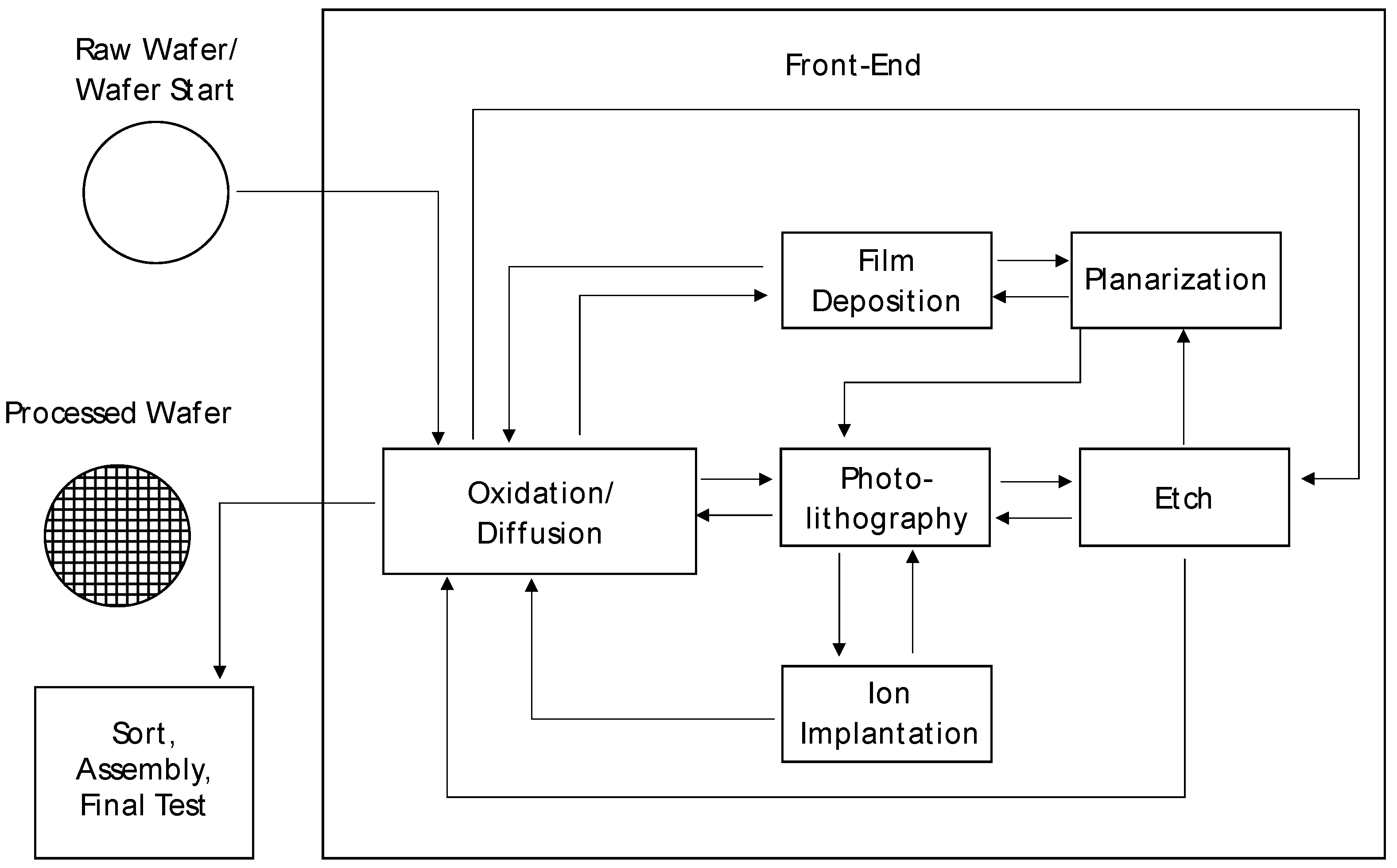
However, besides supply networks, manufacturing is also complex in the semiconductor industry [5,8,9]. The four principal stages of the semiconductor manufacturing process are wafer fabrication and probe, generally referred to as front-end operations, and assembly and test, referred to as back-end operations [4,5]. The front end is usually located in highly industrialized countries, while the back end is often located in countries with low labor costs due to the higher manual effort involved [4]. In wafer fabrication, the most complex part of the overall process, layers of material with different electrical characteristics are built up on a raw wafer. To build these layers, the following process steps have to be performed repeatedly on the wafer: oxidation/diffusion, film deposition, photolithography, etch, ion implantation, and planarization (cf. Figure 1). For a more in-depth technological description of the process steps, please refer to the literature [4,10]. The result of this process, which takes place in a dedicated facility referred to as a wafer fab, is a wafer containing between several hundred and several thousand individual devices [5].
Manufacturing in semiconductor wafer fabs, regarding their manufacturing principle referred to as complex job shops, typically contains more than 100 machines and up to 700 process steps resulting in a lead time of up to 3 months [4]. These complex job shops can be characterized by unequal release dates of the jobs, prescribed due dates of the jobs, reentrant flows of the jobs, different types of processes (lot vs. batch), unequal processing times of jobs at one kind of equipment, sequence-dependent setup times and frequent disturbances (e.g., machine breakdowns) [4,6,8,10]. Complex job shops thus differ significantly from job shops [11].
Because of this complexity, the consequences of changes in manufacturing are difficult to predict. They often lead to unexpected behavior as well as under- or over-steering due to the complexity of the manufacturing system [6,7]. Therefore, simulation has become a proven tool in semiconductor supply network and manufacturing [5,12]. Although there are reference data sets and reference models for semiconductor manufacturing in complex job shops, they often produce entirely different results in scientific publications and are hardly comparable.
Consequently, this leads to the research question of how a reference model could be designed and described in order to enable comparable results. Therefore, this article presents a reference model for semiconductor manufacturing as well as an associated reference implementation. The work contributes to the knowledge base in modeling and simulation of manufacturing systems, especially complex job shops, as well as in production planning and control.
The article is structured as follows. Section 2 presents relevant related work on the modeling and simulation of complex systems, reference models and their implementation as well as reference models for manufacturing. Section 3 then describes the concept of the developed reference model for complex job shop simulation, whereas Section 4 outlines its reference implementation. Experimental results are given in Section 5. The conclusion and future work are outlined in Section 6.
2. Related Work
Related work relevant for this article covers the modeling and simulation of manufacturing systems. This includes the modeling and simulation of complex systems in itself, followed by reference models and their implementation. Furthermore, reference models for manufacturing in general as well as a well-known example in semiconductor manufacturing are described. The outline of the relevant research gap concludes the section.
2.1. Modeling and Simulation of Complex Systems
The formalization of scientific theories is desirable to be explicit, standardized, and objective [13]. Therefore, the modeling of complex systems has become a proven method in many fields, especially in engineering and the mathematical and transportation sciences. Compared to laboratory or pilot plant experiments, it most often provides a relatively low-cost way of gathering information for decision making, especially since the size and complexity of real systems in the areas mentioned rarely allow for analytical solutions to provide the information [14]. For the modeling process, however, some terms and their delimitations need to be understood.
The process of modeling, also referred to as model building, describes the realization of a planned or existing system in a model [15]. Such a system is a set of interrelated elements that are separated from their environment and can be characterized as follows [15]: First, and of utmost importance, by the definition of its borders with the environment and the respective interfaces for material, energy and information exchange as well as the definition of its elements and their sequence structures, denoted by rules and constant or variable attributes. Second, by the relations which connect the system elements among each other. Third, by the states of the elements which are each described by stating the values of all constant and variable attributes. However, generally only a small part of these is relevant to the investigation. Fourth, by the state transitions of the elements as continuous or discrete changes of at least one state variable due to the process running in the system. Furthermore, systems can be characterized by their variability, interconnectedness, and complexity [16]. Many systems are subject to variability, either predictable (e.g., manufacturing volumes) or unpredictable (e.g., machine breakdowns). Furthermore, systems are often interconnected, meaning elements of the system affect one another. Consequently, a change in one part of a system leads to a change in another part of the system. Regarding complexity, a system’s combinatorial complexity and dynamic complexity can be distinguished. Combinatorial complexity is related to the number of elements in a system or the number of combinations of elements that are possible (e.g., order flows in job shops). Dynamic complexity arises from the interaction of components in a system over time and, therefore, is not necessarily related to size. However, systems that are highly interconnected (e.g., job shops) are likely to also display dynamic complexity with the following effects. First, an action has dramatically different effects in the short and long run. Second, an action has a very different set of consequences in one part of the system compared to another. Third, an action leads to non-obvious consequences (counter-intuitive behavior).
A model on the other hand is a simplified reproduction of a planned or existing system [15]. It is characterized by the three criteria mapping, reduction and pragmatism [17]. Mapping describes that a model always represents a natural or an artificial original. However, a model does not capture all attributes of the original, but only those that seem relevant to the model creator or the model user—a reduction. Furthermore, as described by pragmatism, models are not uniquely assigned to their originals. They fulfill their replacement function for certain subjects, within certain time intervals and under restriction to certain mental or actual operations. We can distinguish between conceptual models and simulation models, also referred to as computer models [15,16]. The conceptual model is a non-software-specific description of the model that is to be developed. It contains the objectives, inputs, outputs, content, assumptions and simplifications of the model [16]. In implementation, the conceptual model is, for the purpose of simulation, converted into an executable simulation model. Execution is not strictly limited to computers. However, nowadays most models are executed on a computer using spreadsheets, programming languages or specialist simulation software [15,16].
Simulation is the result of solving the equations of a model, whereas a computer simulation is the result of having a simulation running on a computer [18]. Since nowadays most simulations are executed on a computer, simulation usually refers to a computer simulation. The purpose of simulation is to improve certain target values by varying the parameters with the aim of reaching findings which are transferable to reality [15,19]. Therefore, simulation means running experiments with the model, differentiated by alternatives in a model’s logic and/or input data [16,20]. Input data are typically provided by data sets which are the totality of all data available and necessary for simulation: data for describing reality, which are either recorded by performing measurements and observations of the real system or specified as target values for a planned system [15]. There is a difference between the concepts of static simulation, which imitates a system at a point in time, and dynamic simulation, which imitates a system as it progresses through time. The term simulation is mostly used in the context of dynamic simulation [12,16].
The term simulation is used extensively in manufacturing, ranging from visual simulation of factories or individual machine tools to the stochastic simulation of entire supply networks [19]. The need for simulation results from the fact that many manufacturing systems are interconnected and subject to both variability and complexity (combinatorial and dynamic). In contrast to other modeling approaches (e.g., linear programming or heuristic methods), simulation models can represent the variability, interconnectedness and complexity of a system, and, therefore, predict the system performance with a simulation. Consequently, alternative system designs can be compared and the effect of alternative policies on the system performance determined [16]. Furthermore, simulation models typically need fewer assumptions and are more transparent than other modeling approaches [16]. In addition, compared to experiments with real systems in laboratories or pilot plants, simulation often allows for a time and cost reduction, control of the experimental conditions and even research on non-existing real systems [16]. Therefore, simulation can provide support in the planning, implementation and operation phase of a manufacturing system [21]. However, there are also certain disadvantages of simulations to consider [16]. First, modeling can also be very time-consuming. Second, the required software infrastructure can be expensive. Third, there is a certain risk for overconfidence, meaning that anything produced on a computer is seen to be right. Therefore, when interpreting the results from a simulation, consideration must be given to the validity of the underlying model and the assumptions and simplifications that have been made.
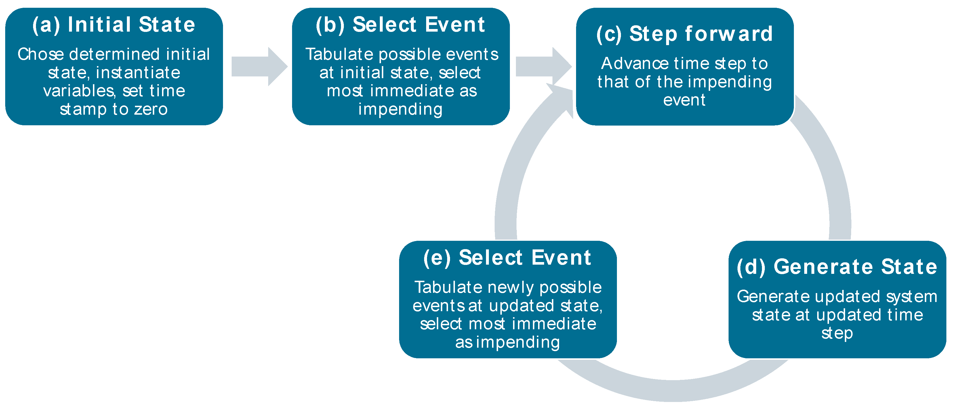
Simulation approaches can be differentiated by their modelling of the progress of time in time-slicing simulation, discrete-event simulation and continuous simulation [16,19]. Discrete-event Simulation (DES), as often used to simulate manufacturing systems, only represents the points in time when the state of the system changes. Therefore, the system is modelled as a series of events as instants in time when a state change occurs. The state of the system is only determined when an event takes place. The time of the simulation run, thus, jumps from one event to the next, whereas the interim state of the system is either assumed to be unchanged or nondeterministic [16,19,25]. Examples of events are incoming customer orders or machines starting to produce [16]. Figure 3 describes the method of DES. Steps (c) to (e) are repeated until the events for the entire timeframe of interest have been generated. However, as the simulation loop can go on forever, it is necessary to establish some terminating conditions [19]. In the understanding of DES above, a state is a description of a situation that is given at a certain point in time [15].
DES for manufacturing sites can be time-consuming to build and is generally slow in execution. However, good accuracy can be achieved [26]. Therefore, simulation and especially DES is receiving a lot of attention in the field of manufacturing systems [19,25]. DES can be applied to different levels: work center, manufacturing site, internal supply network and end-to-end supply network [12]. Hereafter, when referring to simulation, DES of a manufacturing site is meant.
To model a manufacturing site, the following elements could be considered [12]. First, resources including equipment, secondary resources, and operators. Second, products with their associated technologies and work routes. Third, orders, lots, and batches. Fourth, and closely related to the resources, are elements of the control system, i.e., dispatching and batching rules.
2.2. Reference Models and Their Implementation
The architecture of a software system consists of its structures, the decomposition into components, their interfaces and relations among themselves, as well as their constraints [27,28,29]. The behavior of each component is part of the architecture and embodies how elements interact with each other [29]. Consequently, an architecture contains both static and dynamic aspects. It fulfills both the task of a blueprint and that of a flowchart for software [27]. Software architectures are therefore comparable to models (cf. Section 2.1) to a certain extent, and just as there is a need for reference architectures, there is a need for reference models.
A reference model is a model that is intended to have a generally valid character. Most likely, it is created for a whole industry [30]. A reference model presents a set of unifying concepts, axioms and relationships within a particular problem domain, independent of specific standards, technologies, implementations or other concrete details [31]. Therefore, reference models are most likely conceptual models and could serve as a starting point for the development of company-specific models [30].
Reference models can accelerate modeling and increase model quality. This is due to the easier recognition of existing weaknesses in previous processes and typically multiple validation of the reference models. Possible cost savings go hand in hand with a more efficient modeling. Furthermore, reference models allow for a better understanding by providing a standardized conceptual world and a resulting normative effect. Reference models can serve as a testing platform for researchers and, subsequently, to share, replicate and compare results. Therefore, they can also be seen as a bridge between academia and industry [30,32]. However, there is also a tradeoff in the level of abstraction to be managed. Reference models that are too detailed hardly need to be adapted, but they also do not fit the requirements of many companies, so that they are not widely used. If, on the other hand, reference models are too general, then they have to be adapted too much and thus at great expense, so that their use is also called into question. A specific expertise is required for the resulting model adaption. Furthermore, standardization in reference models leads to a possible loss in the representation of strategic competitive advantages and core competencies [30].
Various reference models for manufacturing companies exist, e.g., in the context of supply networks [33,34,35] or manufacturing (cf. Section 2.3). Reference models have proven to be an effective and powerful instrument for manufacturing companies to gain an overview and deeper understanding of their processes, to give orientation for reengineering and optimization, and finally, to configure and control these processes in operation [35].
In computer science, implementation describes the development of a program or subprogram that is executable on a computer [15]. Therefore, it can easily be compared to the steps in modeling and simulation when transferring a conceptual model to a simulation model (cf. Section 2.1) A reference implementation is the implementation of a standard to be used as a definitive interpretation for the requirements in that standard [36]. Reference implementations can serve many purposes, but most importantly they can be used to verify that the standard is implementable and support interoperability testing among other implementations. A reference implementation may or may not have the quality of a commercial product or service that implements the standard [36]. Reference implementations verify that a specification is implementable and serves as so-called gold standard against which other implementations can be measured [37]. This is especially evident for the purpose of reference to compare results as mentioned above. In terms of modeling and simulation, reference implementation means the conversion of a conceptual reference model into an executable reference simulation model.
2.3. Reference Models for Manufacturing
Reference models such as the Reference Architectural Model Industrie 4.0 (RAMI 4.0) [38] are well established to describe software architectures, also for manufacturing companies. Since simulation is of particular importance for decision-making in semiconductor manufacturing, there are several reference models describing its manufacturing process [4]. In their level of detail and inherent capabilities, they usually go well beyond well-known job shop data sets from operations research, e.g., [39,40,41].
MIMAC consists of six wafer fab models with different complexities [42,43]. MiniFab is a model with rather low complexity, focusing on basic principles of complex job shops [44]. A scaled-down model of an existing wafer fab operated by Harris Corporation is described by [45]. A model including automated material handling, SEMATECH 300 mm, is given by [46]. SMT2020, as the most recent model which is also the most complex one, contains a high-volume/low-mix model as well as low-volume/high-mix model [32,47]. A comparison is shown in Table 1.
2.4. MIMAC
While MIMAC has been a widely adopted reference model for the past few years, it is important to note that it is rarely applied in scientific research. In this chapter, we will provide a detailed overview of various reference models that have been utilized in previous studies [47,48]. MIMAC, also known as Measurement and Improvement of Manufacturing Capacity, was originally developed by SE-MATECH in 1995 [42,43]. The model consists of six different wafer fabs, each described by their machines, operators, work routes, rework sequences, and release information. Depending on the specific MIMAC set (ranging from one to six), up to 260 machines in 85 tool groups may be included, visited by up to 21 products in 280 process steps. Data for each model are provided in tabular format, and the level of detail enables the modeling of complex job shop characteristics such as per-lot and per-batch processes, scrap at both wafer and lot levels, rework sequences, batching, and sequence-dependent setup times. It is worth noting that MIMAC utilizes a first-come-first-served approach as the default rule for manufacturing control. However, in this chapter, we will focus on alternative reference models that have been applied in various scientific studies to provide a more comprehensive understanding of simulation methods and their impact on manufacturing processes.
2.5. Research Gap
The MIMAC model has been a major benchmark for semiconductor manufacturing research for several decades. Even today, it remains one of the most widely available models for this type of research [32]. The impact of MIMAC on the simulation community of semiconductor manufacturing has been substantial, as it has led to the use of more realistic simulation models [48]. Consequently, many researchers have used MIMAC over the years in their research [49,50,51]. Despite its widespread use, however, the usage of MIMAC in related works reveals a lack of well-defined assumptions, procedures, and implementation guidelines. This lack of standardization makes it difficult to re-implement the model and makes results obtained from simulations using different implementations of MIMAC not directly comparable. Furthermore, the model’s limited features, such as the absence of lot prioritization (“hot lots”), could also restrict its applications. Therefore, a significant research gap exists in the standardization of the use of the MIMAC model, as well as the identification and implementation of missing features. Addressing this gap would allow for more reliable and comparable simulation results in the semiconductor manufacturing research community and expand the model’s potential applications.
3. Complex Job Shop Simulation
Complex Job Shop Simulation (CoJoSim) is a reference model for semiconductor manufacturing developed by the authors and described hereafter. First, the development approach is outlined including a more specific formulation of the problem. Second, the assumptions made, and, third, the features created are described.
3.1. Approach
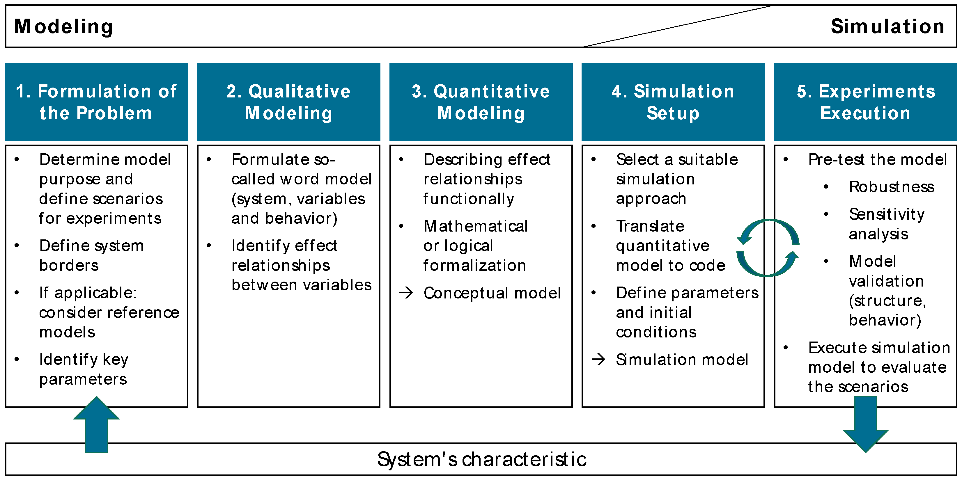
Since existing reference models for manufacturing are subject to certain limitations and, in contrary to their purpose often not comparable, CoJoSim was developed. It is described in detail below to enable comparable simulation results and to be re-implementable at any time by other researchers and practitioners. The approach to developing CoJoSim is based on the steps for modeling and simulation as described in Section 2.1. The problem statement is formulated below. The qualitative and quantitative modeling is described in Section 3.2, Section 3.3 and Section 3.4. The outcome is a conceptual reference model. Based on this, the reference implementation as a simulation model is shown in Section 4. First insights on experimental results are given in Section 5.
The purpose of CoJoSim is to model and simulate a manufacturing system in the semiconductor industry. It can be used to generate data of (e.g., for machine learning applications) as well as to evaluate changes in manufacturing systems (e.g., strategies for production planning and control). Since wafer fabrication is considered the most complex part of semiconductor manufacturing, CoJoSim is limited to this complex job shop environment as the system being modeled. This also serves as the system border. To interact with its environment, CoJoSim needs to provide interfaces for information and (virtual) material flows. Amongst them are incoming orders, manufacturing data and deliveries of finished products. Key parameters for CoJoSim are the structure of the manufacturing system from its elements (e.g., machines, machine groups, products, etc.) and the interaction of these elements (e.g., described by work routes for each product).
3.2. Structure
As described in Section 2.4, MIMAC consists of six models denoted assets. Most popular and most used is MIMAC set one [47], which has therefore been chosen as the basis for our approach. MIMAC set one encompasses two products with their respective work routes, eighty-three machine groups processing lots with a size of forty-eight wafers, batches (with a minimum and a maximum number of lots) and single wafers (one wafer per process) as well as rework sequences and scrap. It is meant to have a total wafer start of 4000 wafers per week, with twice the share of product one compared to product two.
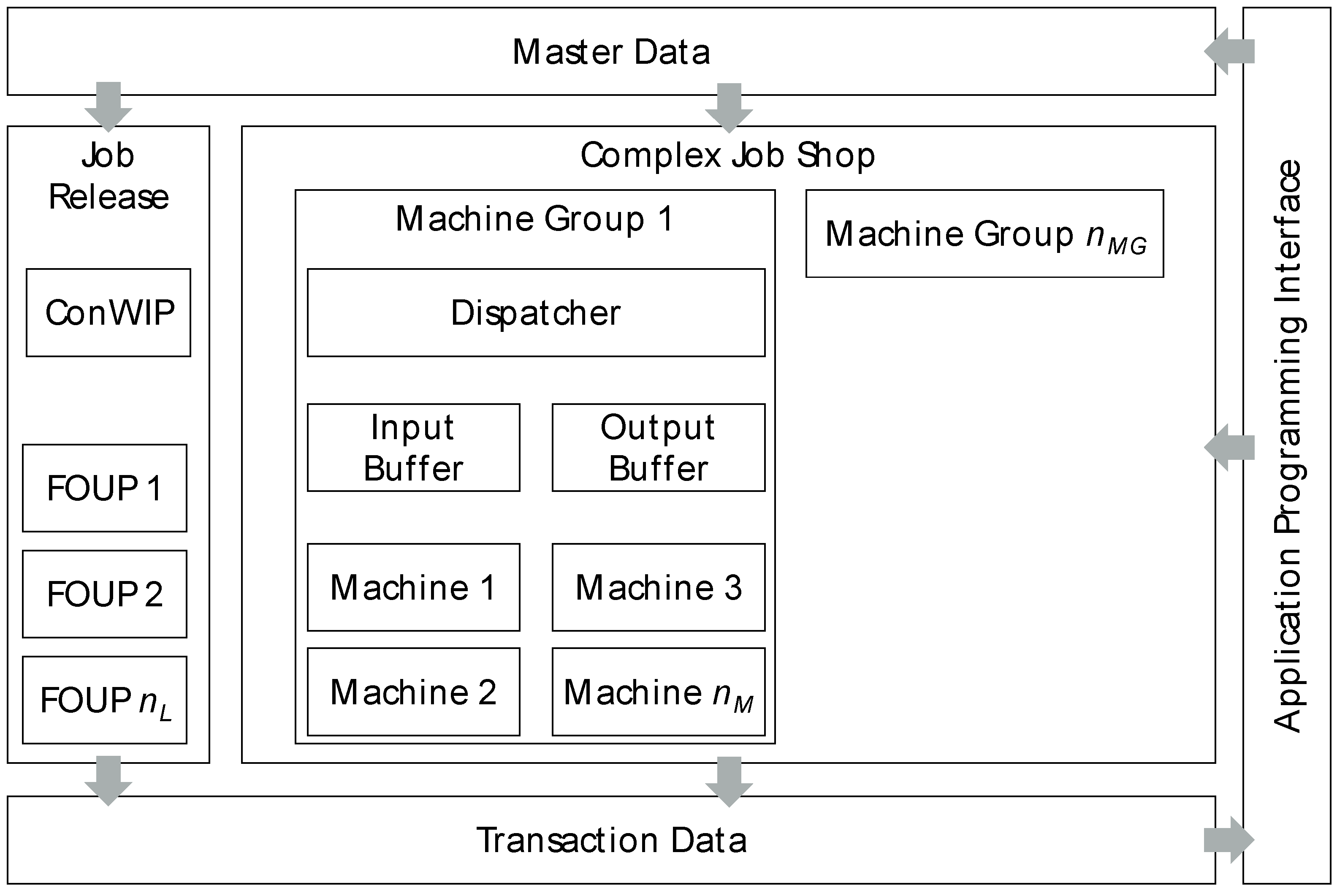
Since not all machine groups were used in MIMAC’s work routes, it was possible to compress CoJoSim to 69 machine groups (nMG). Each machine group consists of an individual number of machines, up to 12 in total (nM). CoJoSim is then parametrized by the described master data of work routes, machine groups and wafer starts resulting from job releases. Therefore, the model could easily be adapted by changing the respective master data. It is therefore very flexibly adaptable to various applications. According to Figure 4, CoJoSim’s conceptual reference model is structured in a module “Job Release” (JRM) and a module “Complex Job Shop” (CJSM) each containing various submodules. When running the implemented simulation model (cf. Section 4 and Section 5), transaction data is generated. All data and modules of CoJoSim could be accessed by an application programming interface (API). This API allows external software to read and write data to the simulation model.
The JRM controls access to the manufacturing system and consists of the subclasses ConWIP control and Front Opening Unified Pod (FOUP). The ConWIP control ensures a consistent work in process in the complex job shop and releases jobs according to a given schedule with associated due dates. Details of ConWIP’s mechanisms can be found in the literature [52]. FOUPs correspond to the transport units for wafers in a semiconductor manufacturing facility. Accordingly, this subclass is instantiated for each job and linked to the work route of the associated product type when released to the complex job shop.
The CJSM comprises the subclass machine group, which is instantiated in frequency of the number of machine groups in the manufacturing system. The machine group, in turn, consists of the subclasses of the dispatcher, the input buffer, the output buffer and the machine. The dispatcher contains manufacturing control with the procedure for selecting the next lot to be processed as soon as a machine becomes available. The input buffer and output buffer represent the stock waiting for processing before the machining process or waiting for transportation after the machining process, respectively. The machine represents the actual machining process, modeled by the setup time and the processing time. The subclass of the machine is instantiated in frequency of the number of parallel machines within the respective machine group ranging from one to nM and could be of one of the following three types:
- PerUnit: Machines of this type process each unit, which are wafers in semiconductor manufacturing, separately.
- PerLot: Machines of this type process each lot in a single rush.
- PerBatch: Machines of this type process batches consisting of a number of lots between a minimum and a maximum number.
3.3. Assumptions
To ensure practical applicability, suitable values and probability distributions for the model assumptions were developed in collaboration with experts from a leading semiconductor manufacturer. While users have the option to modify these values, it is important to note that doing so may result in behavior that deviates from real-world scenarios, such as deadlock situations. Any modifications made to the original assumptions should be carefully evaluated and validated to ensure the model’s reliability and accuracy (cf. Section 2.1).
- CoJoSim’s underlying MIMIAC data set does not define the batching mechanism for PerBatch machine groups exactly. Therefore, a suitable batching mechanism has been developed for CoJoSim jointly with a semiconductor manufacturer. It works as follows: A buffer at the machine group collects lots waiting for either one-third of the processing time or reaching the maximum number of lots for the batch. For two bottleneck processes with a processing time of 22 h and more, waiting time is defined as one-twelfth of processing time. When one of these limits (time or capacity) is reached, all lots of the batch are processed simultaneously by the PerBatch machine group and are subsequently made available in the output buffer for transport.
- In semiconductor manufacturing, an increasing trend towards the automation of transport processes can be observed. To simplify the model, operators were, therefore, analogously to work in [48], not explicitly modeled in CoJoSim. In order to represent the transport processes, transport times are defined for each machine group in each work route. Additionally, transport components such as automated guided vehicles could be modeled separately and integrated using CoJoSim’s API.
- In order to achieve a pragmatic model design, the rework of single wafers and the rework of single lots are combined in one routine in CoJoSim. Rerouting for lots to be reworked is implemented as described by the underlying MIMAC data set. To select lots for rework, the uniform distribution between 0 and 100 is used to compare distribution results with probabilities.
- To reduce CoJoSim’s complexity, scrap of single wafers is not modeled. Instead, scrap of single lots is considered with a higher frequency. Lots that are selected as scrap are separated after each process step and collected in separate storages. To select lots for scrap, the uniform distribution between 0 and 100 is used to compare distribution results with probabilities.
3.4. Features
In order to ensure the applicability of CoJoSim in state-of-the-art applications, several features have been designed to implement the structure and assumptions as well as to complement them.
- Different applications require different data and mechanisms. Furthermore, boundary conditions for applications and their simulation models may change over time. CoJoSim is therefore designed modularly to allow the addition, modification, or removal of modules and subclasses (cf. Section 3.2) at any time.
- An API enables CoJoSim to interact with its environment allowing external software to write master data to the model (e.g., work routes), to adapt the structure of the complex job shop environment simulated (e.g., machine groups) or its mechanisms (e.g., dispatching methods) and to read transaction data from the model (e.g., delivery dates of finished lots).
- As described in Section 3.2, CJSM is structured by an adjustable number of machine groups. Within a machine group, there are one to nM machines which are of type PerUnit, PerLot or PerBatch. Within one machine group, there can only be a single machine type. It is the dispatcher’s task, if a machine of the machine group becomes available, to select a unit/lot/batch to process next. Due to its modular design, common dispatching rules according to the literature [53] are considered by default in the dispatcher and could be selected before running the model. They could be easily complemented by additional dispatching rules or other manufacturing control approaches. This can overcome the research gap that, unlike with the underlying MIMAC, an explicit prioritization of lots, rather than a first-come-first-serve rule, is available.
- A particular focus of CoJoSim is to comprehensively collect transaction data. Therefore, whenever a lot is entering or leaving a machine group, transaction data is updated. All data is stored in a so-called manufacturing feedback data table, structured according to Table 3. The data could be used within CoJoSim, as well as accessed by the API. The manufacturing feedback data enables (external) scripts to analyze key performance indicators (e.g., adherence to schedule, yield, etc.) via the API.
4. Reference Implementation
This section shows the reference implementation for CoJoSim. First, benefits of a reference implementation are described. Second, specifics of this reference implementation are outlined.
4.1. Benefits of a Reference Implementation for CoJoSim
Benefits of reference implementations are to some extent comparable to the benefits of reference models as described in Section 2.2. Thus, reference implementations can significantly accelerate the implementation and application of reference models and, therefore, may achieve significant cost savings. Even more than reference models, reference implementations could serve as testing platforms and a bridge between academia and industry. In addition, a reference implementation ensures that a reference model is implementable, bridging the gap between quantitative modeling and simulation setup (cf. Figure 2). Furthermore, a reference implementation could serve as a gold standard against which other implementations can be measured.
4.2. Specifics of CoJoSim’s Reference Implementation
As a foundational step, a simulation software to implement the reference model had to be chosen first. SimPy [54] is widely used in academia for implementing simulation models. However, to ensure applicability, CoJoSim should be implemented in a simulation software which is also widely used in industry. Therefore, it was chosen to implement in Siemens Tecnomatix Plant Simulation (PS), version 14. (Even though the model was originally implemented in version 14 of Plant Simulation, it also runs flawlessly with the current version 17. If there are no drastic changes, it is expected to run in future versions as well.) As one of the market leaders, PS offers an object-oriented structure for mapping classes and objects in a DES, numerous predefined building blocks and the possibility to extend the building blocks using the built-in SimTalk programming language. PS can be controlled through external software by means of a component object model (COM) interface, and data can be exported, among other things, in open formats as comma-separated values [55]. CoJoSim’s API uses both possibilities. Using the COM interface, methods within the implementation in PS can be triggered (marked by a blue “M” in a gray box in the following figures), which either return smaller data sets or nothing. Additionally, the export of larger data sets is also triggered by the COM interface and then actually exported as comma-separated values.
Since DES is well suited for simulating manufacturing systems, CoJoSim was implemented in such a way. The process of implementing was based on the literature (cf. Section 2.1, especially [14,16]). Bangsow [55] was consulted for specifics of PS. Basically, all elements are implemented in such a way that these are classes that can be instantiated in the number required in each case. If available, existing building blocks of PS were used and adapted. If unavailable, these were complemented by methods written in the PS-integrated SimTalk programming languages.
Based on the structure of CoJoSim (cf. Section 3.2), “Wafers” and “FOUPs” are generators, generating PS-elements entities (wafers) and carriers (FOUPS) which are then combined. On a given schedule, they are associated with a product type and its respective work route and released to the complex job shop (“Release”). The release includes the ConWIP control ensuring a consistent work in process in the complex job shop. Additional products could be easily added by adding further work routes which are structured as described in Section 3.4.
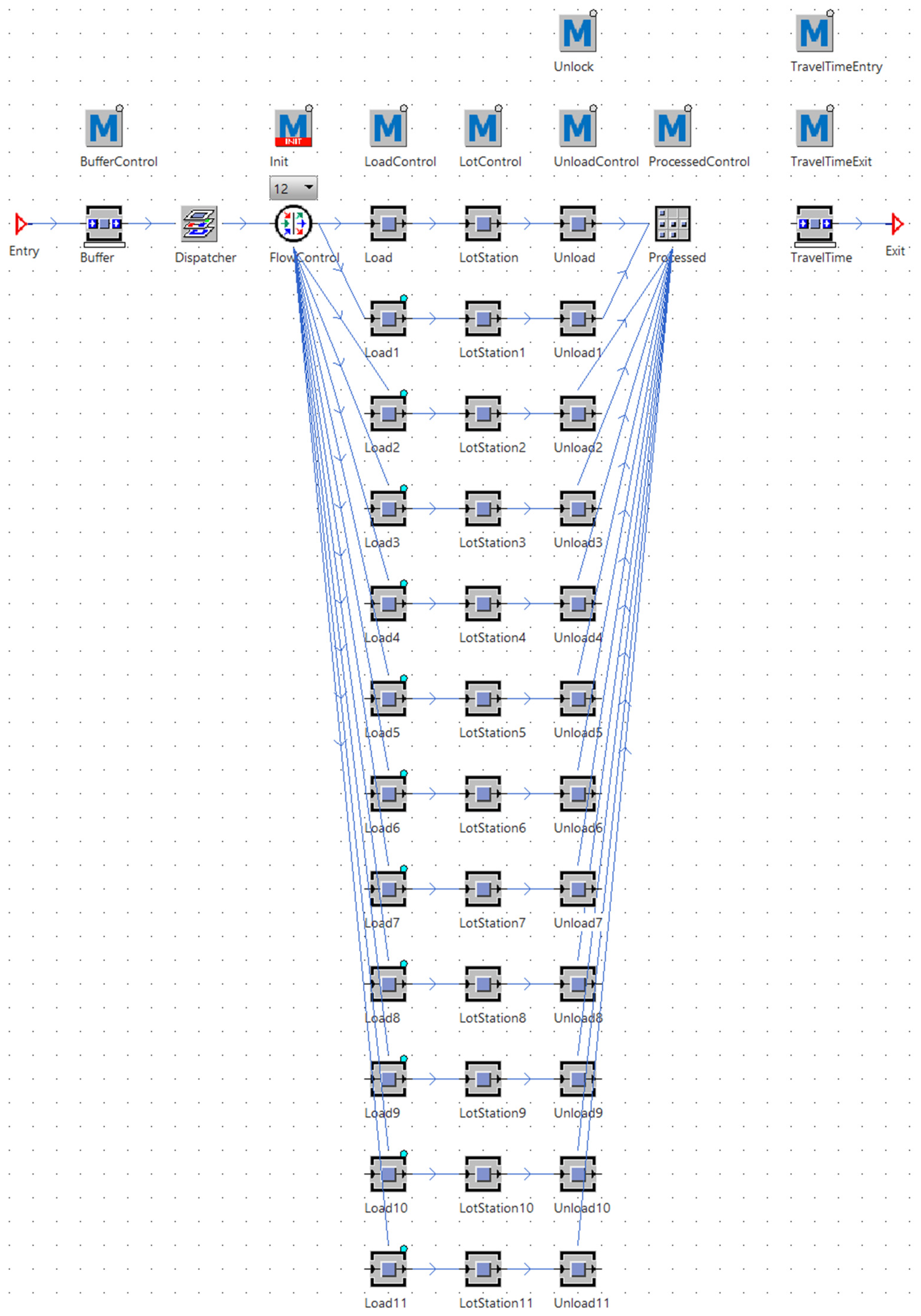
As described in Section 3.2, the CJSM consists of machine groups. These machine groups are the most complex part in implementing CoJoSim in PS since they consist of multiple building blocks and methods (cf. Figure 5). Since the underlying MIMAC specifies one to twelve machines per machine group, a flow control for up to twelve machines is implemented. When instantiated, the number of machines in this specific machine group can be selected. Each machine then has a load station, a process station and an unload station. These are parametrized by the product’s work route with load time, process time and unload time (cf. Section 3.4). Additionally, the machine group has an input buffer, an output buffer with processed wafers and a transport facility for the next operation in the work route. Several methods had to be implemented to control all necessary building blocks. Last but not least is the dispatcher’s task, which will be described in the following paragraph, which is to, if a machine of the machine group becomes available, select a unit/lot/batch to process next.
A key element of the dispatcher is the “DispatchmentControl” method. In a switch-case-instruction it contains all implemented dispatching rules (cf. Section 3.4) which can be modularly complemented by additional dispatching rules or other dispatching methods. For each machine group, the dispatching rule to be used can be individually selected before running the simulation model. The dispatching rule then selects the next job to be processed at a machine which has become available. To save calculation time in the simulation model, only this job with the highest priority is selected—no further sequencing takes place.
However, there was also a limitation in PS which needed to be considered when implementing CoJoSim. CoJoSim’s underlying MIMAC data set contains a mean time between failure (MTBF) and a mean time to repair (MTTR) for each machine group. PS, however, allows for dealing with MTTR and availability (as a percentage) only. Therefore, according to [55], availability was calculated as MTBF/(MTBF + MTTR).
The results of this study were obtained through simulation runs for each test instance, where computing speed is an essential factor. Our findings demonstrate that the computational cost was insignificant, with simulation runs completing in just a few seconds. This highlights the simulation tool’s efficiency and gives us confidence in the accuracy of the results. The study suggests that the simulation tool has potential for use in large-scale semiconductor simulations, where efficiency is crucial.
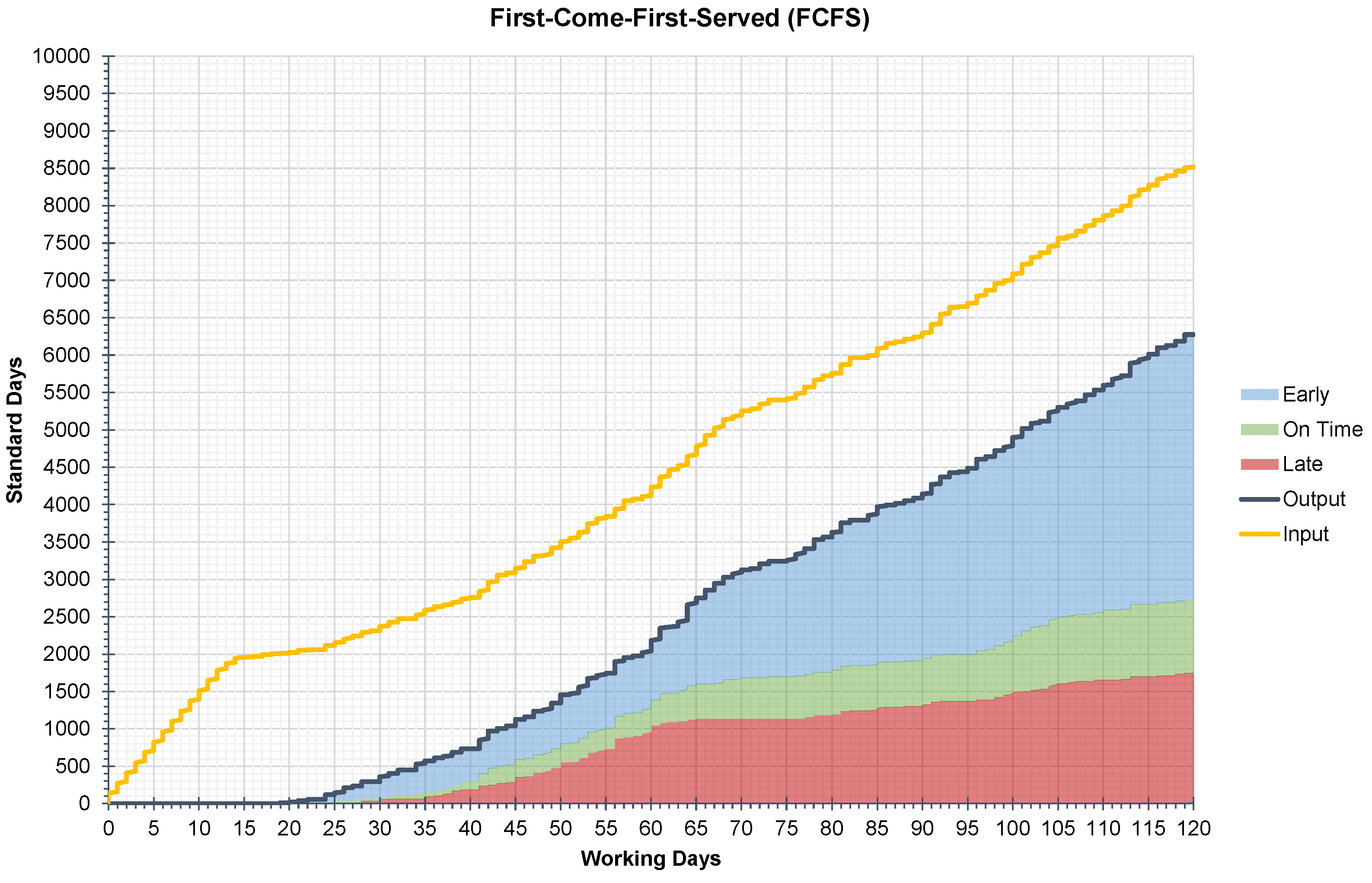
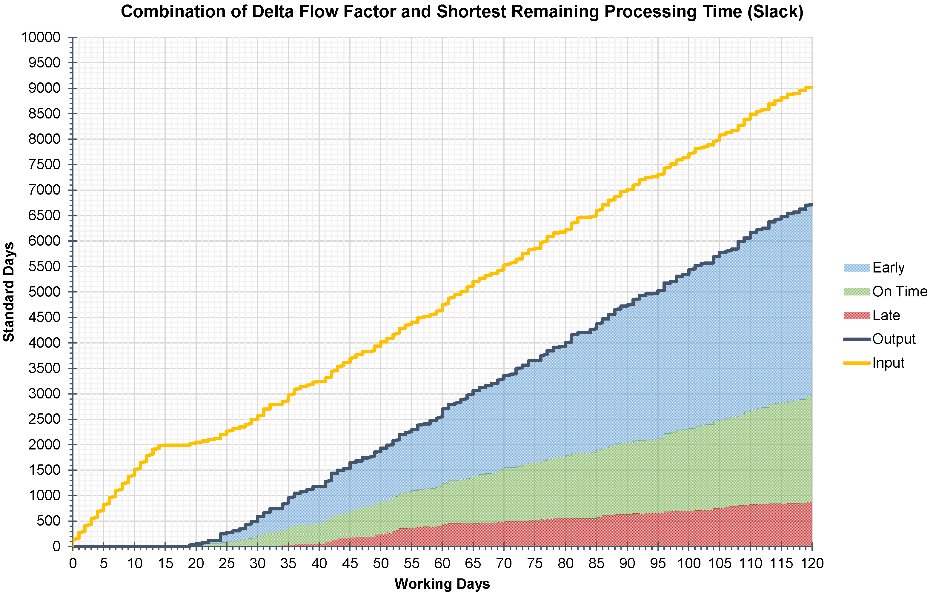
5. Application
The reference implementation of CoJoSim was applied to evaluate and compare different dispatching rules. For this purpose, 120 days were simulated and the manufacturing feedback data were continuously recorded to calculate key performance indicators (KPIs). These KPIs were then visualized and analyzed using throughput diagrams [56]. Since these diagrams focus on quantities without considering adherence to delivery dates, the output during the reference period in the throughput diagrams was split and colored for jobs that were early, late, and on time. To calculate adherence to delivery dates, early jobs and on-time jobs were summed. For more information on calculating KPIs and logistic targets, as well as analyzing throughput diagrams, the literature [7,56] can be referred to.In the application, five dispatching rules were evaluated and combined. The first rule used was first-come-first-served (FCFS), which was used as a reference and is also the basic way of prioritization in the underlying MIMAC. The second rule is priority classes (PC), a rather simple dispatching rule. The third rule is delta flow factor (DFF), which considers the tardiness of the jobs. The fourth rule is shortest remaining processing time (SRPT), which prioritizes jobs with a higher degree of completion. The fifth rule is a slack-based dispatching rule (Slack), which combines DFF and SRPT. Figure 6 shows the throughput diagram for FCFS, which serves as a reference for comparing the other four dispatching rules. Table 4 presents the results of the four simulated dispatching rules for prioritizing jobs in CoJoSim. FCFS has a mean throughput of 6275 standard days (for a 120 working days simulation duration) and a mean adherence to delivery dates of 71.36% and is used as a reference. The following dispatching rules have the common objective of influencing and improving adherence to delivery dates compared to this reference. With DFF and SRPT, mean throughput and mean adherence to delivery dates can be slightly increased compared to the reference. A significant improvement is possible with PC, and the best results are achieved with Slack. An improvement in adherence to delivery dates of almost 15 percentage points was achieved by Slack compared to the reference. The throughput diagram for Slack is shown in Figure 7.
When reviewing the results, it is remarkable that PC, a rather simple dispatching rule, performs comparatively well. This is likely due to matching prioritization at bottle-necks. However, it is also clear that this dispatching rule is too simplistic for real-world applications. DFF and SRPT both improve performance compared to the reference only slightly. However, combining both with Slack achieves the best results in the analyzed application. This observation can presumably be explained by the fact that meeting deliv-ery dates plays a significantly smaller role at the beginning of the work route than at the end and that jobs with a higher degree of completion tend to be prioritized by Slack. Therefore, a hierarchy of different dispatching rules is usually used in practice as well [57]. Other important parameters in production control, such as machine utilization rate or work-in-progress inventories, were not analyzed in this study. Future research could focus on evaluating the impact of these parameters on the performance of different dispatching rules in production control.
6. Conclusions and Outlook
The market environment in which manufacturing companies operate is becoming increasingly volatile, uncertain, complex, and ambiguous. This increases the need to constantly optimize manufacturing, especially the achievement of logistic targets by production planning and control. Due to the complex nature of the manufacturing process, con-sequences of changes in manufacturing are difficult to predict in semiconductor manufacturing. Consequently, simulation has become a proven tool in semiconductor manufacturing. Although there are reference data sets and reference models for semiconductor manufacturing in complex job shops, they often produce different results and are hardly comparable. Therefore, this article describes CoJoSim, our approach for a reference model for semiconductor manufacturing as well as an associated reference implementation. The reference implementation allows for a significant acceleration of the implementation and application of the reference model. It could serve as a testbed and as a gold standard against which other implementations can be measured. CoJoSim was applied to evaluate different dispatching rules. In a comparison of five dispatching rules, an improvement in the adherence to delivery dates of almost fifteen percentage points was achieved compared to the reference.
To extend knowledge in the research field, the authors are currently focusing on the following aspects. First, we are evaluating the application of CoJoSim in further use cases and with further dispatching rules. For example, the dispatching rules investigated so far have not yet optimized the setup time. Particularly with higher product variance, the setup time at machines could have a significant influence on the adherence to delivery dates and the throughput. The influence of setup time optimization should therefore still be investigated. Second, CoJoSim can also be combined and applied with dispatching methods that integrate not only manufacturing but also the supply network. Therefore, it could serve as an environment to train reinforcement-learning-based agents optimizing production planning and control of semiconductor manufacturers when reacting to events in their supply network [58].
Author Contributions
D.B. managed the project, worked on the conceptualization, the investigation of the research subject, the design of the methodology, the development of the general structure, and wrote the manuscript. A.S. (Andreas Schlereth) implemented the first iteration of the software model based on the underlying data set. D.U. conceptualized the dispatcher component, further developed the design of the software model and implemented further iterations of the software model. Furthermore, he conducted the experiments for the application described. D.B. supervised the work of D.U. and A.S. (Andreas Schlereth). T.B. and A.S. (Alexander Sauer) supervised the work of D.B. All authors and supervisors provided critical feedback and helped shape the research, analysis, and manuscript. All authors have read and agreed to the published version of the manuscript.
Funding
Parts of this work have been performed in the project Power Semiconductor and Electronics Manufacturing 4.0 (SemI40), under grant agreement No 692466. The project has been co-funded by grants from Austria, Germany, Italy, France, Portugal and—Electronic Component Systems for European Leadership Joint Undertaking (ECSEL JU).
Institutional Review Board Statement
Not applicable.
Informed Consent Statement
Not applicable.
Data Availability Statement
Not applicable.
Acknowledgments
The authors sincerely thank Axel Bruns (Fraunhofer IPA) and Thomas Ponsignon (Infineon Technologies AG) for the fruitful discussions in conceptualizing and implementing certain parts of this model.
Conflicts of Interest
The authors declare no conflict of interest. The funders had no role in the design of the study; in the collection, analyses, or interpretation of data; in the writing of the manuscript; or in the decision to publish the results.
References
- Mack, O.; Khare, A. Perspectives on a VUCA World. In Managing in a VUCA World; Mack, O., Khare, A., Krämer, A., Burgartz, T., Eds.; Springer: Cham, Switzerland, 2016; pp. 3–19. ISBN 978-3-319-16888-3. [Google Scholar]
- Bauernhansl, T.; Hörcher, G.; Bressner, M.; Röhm, M. MANUFUTURE-DE: Identification of Priority Research Topics for the Sustainable Development of European Research Programs for the Manufacturing Industry until 2030; Fraunhofer IPA: Stuttgart, Germany, 2018. [Google Scholar]
- Aelker, J.; Bauernhansl, T.; Ehm, H. Managing Complexity in Supply Chains: A Discussion of Current Approaches on the Example of the Semiconductor Industry. Procedia CIRP 2013, 7, 79–84. [Google Scholar] [CrossRef]
- Mönch, L.; Fowler, J.W.; Mason, S.J. Production Planning and Control for Semiconductor Wafer Fabrication Facilities: Modeling, Analysis, and Systems; Springer: New York, NY, USA, 2013; ISBN 9781461444718. [Google Scholar]
- Mönch, L.; Uzsoy, R.; Fowler, J.W. A survey of semiconductor supply chain models part I: Semiconductor supply chains, strategic network design, and supply chain simulation. Int. J. Prod. Res. 2018, 56, 4524–4545. [Google Scholar] [CrossRef]
- Mönch, L.; Fowler, J.W.; Dauzère-Pérès, S.; Mason, S.J.; Rose, O. A survey of problems, solution techniques, and future challenges in scheduling semiconductor manufacturing operations. J. Sched. 2011, 14, 583–599. [Google Scholar] [CrossRef]
- Lödding, H. Handbook of Manufacturing Control: Fundamentals, Description, Configuration; Springer: Berlin/Heidelberg, Germany, 2013; ISBN 978-3-642-24457-5. [Google Scholar]
- Waschneck, B.; Bauernhansl, T.; Altenmüller, T.; Kyek, A. Production Scheduling in Complex Job Shops from an Industry 4.0 Perspective: A Review and Challenges in the Semiconductor Industry. In Proceedings of the International Conference on Knowledge Technologies and Data-Driven Business (i-KNOW 2016), Graz, Austria, 18–19 October 2016. [Google Scholar]
- ElMaraghy, W.; ElMaraghy, H.; Tomiyama, T.; Monostori, L. Complexity in engineering design and manufacturing. CIRP Ann. Manuf. Technol. 2012, 61, 793–814. [Google Scholar] [CrossRef]
- Uzsoy, R.; Lee, C.-Y.; Martin-Vega, L.A. A Review of Production Planning and Scheduling Models in the Semiconductor Industry: Part I: System Characteristics, Performance Evaluation and Production Planning. IIE Trans. 1992, 24, 47–60. [Google Scholar] [CrossRef]
- Pinedo, M. Scheduling: Theory, Algorithms, and Systems, 5th ed.; Springer: Cham, Switzerland, 2016; ISBN 978-3-319-26578-0. [Google Scholar]
- Fowler, J.W.; Mönch, L.; Ponsignon, T. Discrete-event simulation for semiconductor wafer fabrication facilities: A tutorial. Int. J. Ind. Eng. Theory Appl. Pract. 2015, 22, 661–682. [Google Scholar]
- Suppes, P. The Desirability of Formalization in Science. J. Philos. 1968, 65, 651. [Google Scholar] [CrossRef]
- Fishman, G.S. Discrete-Event Simulation: Modeling, Programming, and Analysis; Springer: New York, NY, USA, 2001; ISBN 978-0-387-95160-7. [Google Scholar]
- VDI. Simulation of Systems in Materials Handling, Logistics and Production: Terms and Definitions; Beuth: Berlin, Germany, 2018. [Google Scholar]
- Robinson, S. Simulation: The Practice of Model Development and Use; John Wiley & Sons: Chichester, UK, 2004; ISBN 0-470-84772-7. [Google Scholar]
- Stachowiak, H. Allgemeine Modelltheorie; Springer: Wien, Austria, 1973; ISBN 3-211-81106-0. [Google Scholar]
- Durán, J.M. What is a Simulation Model? Minds Mach. 2020, 30, 301–323. [Google Scholar] [CrossRef] [Green Version]
- Chatti, S.; Laperrière, L.; Reinhart, G.; Tolio, T. CIRP Encyclopedia of Production Engineering, 2nd ed.; Springer: Berlin/Heidelberg, Germany, 2019; ISBN 978-3-662-53120-4. [Google Scholar]
- Schriber, T.J.; Brunner, D.T.; Smith, J.S. Inside discrete-event simulation software: How it works and why it matters. In Proceedings of the 2014 Winter Simulation Conference (WSC 2014), Savanah, GA, USA, 7–10 December 2014; pp. 132–146, ISBN 978-1-4799-7486-3. [Google Scholar]
- VDI. Simulation of Systems in Materials Handling, Logistics and Production: Fundamentals; Beuth: Berlin, Germany, 2014. [Google Scholar]
- Forrester, J.W. Industrial Dynamics; MIT Press: Cambridge, UK, 1961. [Google Scholar]
- Sterman, J.D. Business Dynamics: Systems Thinking and Modeling for a Complex World; Irwin/McGraw-Hill: Boston, MA, USA, 2000; ISBN 978-0-07-231135-8. [Google Scholar]
- Bossel, H. Modellbildung und Simulation: Konzepte, Verfahren und Modelle zum Verhalten Dynamischer Systeme, 2nd ed.; Veränderte Auflage; Vieweg & Teubner: Wiesbaden, Germany, 1994; ISBN 978-3-322-90520-8. [Google Scholar]
- Negahban, A.; Smith, J.S. Simulation for manufacturing system design and operation: Literature review and analysis. J. Manuf. Syst. 2014, 33, 241–261. [Google Scholar] [CrossRef]
- Fowler, J.W.; Rose, O. Grand Challenges in Modeling and Simulation of Complex Manufacturing Systems. Simulation 2004, 80, 469–476. [Google Scholar] [CrossRef]
- Starke, G. Effektive Softwarearchitekturen: Ein praktischer Leitfaden, 8th ed.; überarbeitete Auflage; Hanser: München, Germany, 2018; ISBN 978-3-446-45207-7. [Google Scholar]
- Bass, L.; Clements, P.; Kazman, R. Software Architecture in Practice, 3rd ed.; Addison-Wesley/Pearson: Upper Saddle River, NJ, USA, 2013; ISBN 978-0-321-81573-6. [Google Scholar]
- Kruchten, P.B. The 4+1 View Model of architecture. IEEE Softw. 1995, 12, 42–50. [Google Scholar] [CrossRef] [Green Version]
- Krcmar, H. Informationsmanagement, 6th ed.; Überarbeitete Auflage; Springer Gabler: Berlin/Heidelberg, Germany, 2015; ISBN 978-3-662-45863-1. [Google Scholar]
- Nakagawa, E.Y.; Oliveira Antonino, P.; Becker, M. Reference Architecture and Product Line Architecture: A Subtle But Critical Difference. In Software Architecture; Crnkovic, I., Gruhn, V., Book, M., Eds.; Springer: Berlin/Heidelberg, Germany, 2011; pp. 207–211. ISBN 978-3-642-23797-3. [Google Scholar]
- Hassoun, M.; Kopp, D.; Monch, L.; Kalir, A. A New High-Volume/Low-Mix Simulation Testbed for Semiconductor Manufacturing. In Proceedings of the 2019 Winter Simulation Conference (WSC 2019), National Harbor, MD, USA, 8–11 December 2019; pp. 2419–2428, ISBN 978-1-7281-3283-9. [Google Scholar]
- Ehm, H.; Wenke, H.; Monch, L.; Ponsignon, T.; Forstner, L. Towards a supply chain simulation reference model for the semiconductor industry. In Proceedings of the 2011 Winter Simulation Conference (WSC 2011), Phoenix, AZ, USA, 11–14 December 2011; pp. 2119–2130, ISBN 978-1-4577-2109-0. [Google Scholar]
- Jain, S. A conceptual framework for supply chain modelling and simulation. IJSPM 2006, 2, 164. [Google Scholar] [CrossRef]
- Rabe, M.; Jaekel, F.; Weinaug, H. Reference Models for Supply Chain Design and Configuration. In Proceedings of the 2006 Winter Simulation Conference (WSC 2006), Monterey, CA, USA, 3–6 December 2006; pp. 1143–1150, ISBN 1-4244-0501-7. [Google Scholar]
- NIST. Supplemental Information for the Interagency Report on Strategic U.S. Government Engagement in International Standardization to Achieve U.S. Objectives for Cybersecurity; NIST: Gaithersburg, MD, USA, 2015; Volume 2, NISTIR 8074.
- Curran, P. Conformance Testing: An Industry Perspective; Sun Microsystems: Santa Clara, CA, USA, 2003. [Google Scholar]
- Hankel, M. The Reference Architectural Model Industrie 4.0 (RAMI 4.0); ZVEI: Frankfurt, Germany, 2015. [Google Scholar]
- Fisher, H.; Thompson, G.L. Probabilistic learning combinations of local job shop scheduling rules. In Industrial Scheduling; Muth, J.F., Thompson, G.L., Winters, P.R., Eds.; Prentice-Hall: Englewood Cliffs, NJ, USA, 1963; pp. 225–251. [Google Scholar]
- Applegate, D.; Cook, W. A Computational Study of the Job-Shop Scheduling Problem. ORSA J. Comput. 1991, 3, 149–156. [Google Scholar] [CrossRef]
- Lawrence, S. Resouce Constrained Project Scheduling: An Experimental Investigation of Heuristic Scheduling Techniques (Supplement); Carnegie Mellon University: Pittsburgh, PA, USA, 1984. [Google Scholar]
- Feigin, G.; Fowler, J.W.; Robinson, J.; Leachman, R. Semiconductor Wafer Manufacturing Data Format Specification: SEMATECH Technical Report; SEMATECH: Austin, TX, USA, 1994. [Google Scholar]
- Fowler, J.W.; Robinson, J. Measurement and Improvement of Manufacturing Capacity (MIMAC): SEMATECH Final Report; SEMATECH: Austin, TX, USA, 1995. [Google Scholar]
- Spier, J.; Kempf, K. Simulation of Emergent Behavior in Manufacturing Systems. In Proceedings of the IEEE/SEMI Advanced Semiconductor Manufacturing Conference and Workshops, Cambridge, MA, USA, 13–15 November 1995; pp. 90–94. [Google Scholar]
- Kayton, D.; Teyner, T.; Schwartz, C.; Uzsoy, R. Focusing Maintenance Improvement Efforts in a Wafer Fabrication Facility Operating under the Theory of Constraints. Prod. Inventory Manag. J. 1997, 38, 51–57. [Google Scholar]
- Campbell, E.; Ammenheuser, J. 300 mm Factory Layout and Material Handling Modeling: Phase II Report; SEMATECH: Austin, TX, USA, 2000. [Google Scholar]
- Kopp, D.; Hassoun, M.; Kalir, A.; Monch, L. SMT2020—A Semiconductor Manufacturing Testbed. IEEE Trans. Semicond. Manufact. 2020, 33, 522–531. [Google Scholar] [CrossRef]
- Hassoun, M.; Kalir, A. Towards a new simulation testbed for semiconductor manufacturing. In Proceedings of the 2017 Winter Simulation Conference (WSC 2017), Las Vegas, NV, USA, 3–6 December 2017; pp. 3612–3623. [Google Scholar]
- Yu, Q.; Yang, H.; Lin, K.-Y.; Li, L. A self-organized approach for scheduling semiconductor manufacturing systems. J. Intell. Manuf. 2021, 32, 689–706. [Google Scholar] [CrossRef]
- Ziarnetzky, T.; Monch, L.; Uzsoy, R. Simulation-Based Performance Assessment of Production Planning Models With Safety Stock and Forecast Evolution in Semiconductor Wafer Fabrication. IEEE Trans. Semicond. Manufact. 2020, 33, 1–12. [Google Scholar] [CrossRef]
- Shin, J.; Grosbard, D.; Morrison, J.R.; Kalir, A. Decomposition without aggregation for performance approximation in queueing network models of semiconductor manufacturing. Int. J. Prod. Res. 2019, 57, 7032–7045. [Google Scholar] [CrossRef]
- Hopp, W.J.; Spearman, M.L. Factory Physics, 3rd ed.; McGraw-Hill/Irwin: Boston, MA, USA, 2008; ISBN 978-0072824032. [Google Scholar]
- Gupta, A.K.; Sivakumar, A.I. Job shop scheduling techniques in semiconductor manufacturing. Int. J. Adv. Manuf. Technol. 2006, 27, 1163–1169. [Google Scholar] [CrossRef]
- Müller, K.; Vignaux, T.; Scherfke, S.; Lünsdorf, O. SimPy—Discrete Event Simulation for Python. Available online: https://simpy.readthedocs.io/en/4.0.1/ (accessed on 11 November 2022).
- Bangsow, S. Tecnomatix Plant Simulation: Modeling and Programming by Means of Examples; Springer: Berlin/Heidelberg, Germany, 2015; ISBN 978-3-319-19502-5. [Google Scholar]
- Nyhuis, P.; Wiendahl, H.-P. Fundamentals of Production Logistics; Springer: Berlin/Heidelberg, Germany, 2009; ISBN 978-3-540-34210-6. [Google Scholar]
- Fordyce, K.; Milne, J.R.; Wang, C.-T.; Zisgen, H. Modeling and Integration of Planning, Scheduling and Equipment Configuration in Semiconductor Manufacturing: Part I—Review of Successes and Opportunities. Int. J. Ind. Eng. Theory Appl. Pract. 2015, 22, 601–607. [Google Scholar] [CrossRef]
- Bauer, D.; Bauernhansl, T.; Sauer, A. Improvement of Delivery Reliability by an Intelligent Control Loop between Supply Network and Manufacturing. Appl. Sci. 2021, 11, 2205. [Google Scholar] [CrossRef]
Figure 1.
Process steps in a wafer fab [4].
Figure 1.
Process steps in a wafer fab [4].

Figure 2.
Steps for modelling and simulation.

Figure 3.
Method of discrete-event simulation (adapted from [19]).
Figure 3.
Method of discrete-event simulation (adapted from [19]).

Figure 4.
Structure of CoJoSim.

Figure 5.
Implementation of the machine group.

Figure 6.
Throughput diagram for first-come-first-served.

Figure 7.
Throughput diagram for the combination of delta flow factor and shortest remaining processing time.
Figure 7.
Throughput diagram for the combination of delta flow factor and shortest remaining processing time.


Table 1.
Comparison of reference models for semiconductor manufacturing.
| Model | MIMAC | MiniFab | Harris | SEMATECH 300 mm | SMT2020 |
|---|---|---|---|---|---|
| No. of machines | up to 260 | 5 | 12 | 275 | 1043 |
| No. of machine groups | up to 85 | 3 | 11 | 103 | 105 |
| No. of products | up to 21 | 2 | 3 | 1 | 10 |
| No. of process steps | up to 280 | 6 | up to 22 | 364 | up to 632 |
| Implementation described | No | No | No | No | No |
Table 2.
Structure of work routes.
| Column | Description |
|---|---|
| OperationNumber | This unique identifier links machine groups with respective parameters for a given product in a work route. Additionally, it also indicates progress by its ascending sorting, which, however, does not increase linearly in terms of time. |
| MachineGroup | This field links the operation to be specified to a machine group. Due to reentrant flows in a complex job shop, machine groups are likely to appear multiple times in a work route. |
| LoadTime | Setup time for loading the unit/lot/batch. |
| UnitProcessTime | Raw process time for operations, which are executed on machine groups of the type PerUnit. |
| LotProcessTime | Raw process time for operations, which are executed on machine groups of the type PerLot. |
| BatchProcessTime | Raw process time for operations, which are executed on machine groups of the type PerBatch. |
| UnloadTime | Setup time for unloading the unit/lot/batch. |
| TransportTime | Transport time between the current and the next operation with respect to their associated machine groups. |
Table 3.
Structure of manufacturing feedback data.
| Column | Type | Description |
|---|---|---|
| Identifier | String | Since a new row is added for each operation, this identifier allows a clear allocation. It is structured as follows: ProductType_LotNumber_OperationNumber |
| LotNumber | Integer | Unique identifier for a lot. |
| OperationNumber | Integer | Unique identifier for an operation number corresponding to a work route. |
| MachineGroup | String | Identifier for a machine group at which the lot has been processed while collecting these transaction data. |
| EntryTime | Time | Timestamp when the lot entered the input buffer of the machine group. |
| ExitTime | Time | Timestamp when the lot exited the output buffer of the machine group. |
| OperationalCycleTime | Time | A planning value containing the cycle time for the current operation. |
| ReleaseCycleTime | Time | A planning value containing the total cycle time of a lot, planned when the lot was released to the complex job shop. |
| PlannedCycleTime | Time | A planning value containing the total cycle time of a lot as currently planned. |
| MeasuredCycleTime | Time | A measured value containing a lot’s current cycle time. |
| PlannedRemaining CycleTime | Time | A planning value containing the remaining cycle time of a lot. |
| MeanPlannedRaw ProcessTime | Time | A planning value containing the process time for the current operation. |
| CumulatedRaw ProcessTime | Time | Cumulated raw process time since the lot was released into the complex job shop. |
| DegreeOfCompletion | Float | The degree of completion is a percentage measure of a lot’s progress and is calculated by the ratio of already completed process time to the total process time. |
| ProductionStart | Time | Timestamp when the lot was released into the complex job shop. |
| ProductionStop | Time | Timestamp when the lot exited the complex job shop. |
| ProductionFinished | Boolean | Boolean flag which is set true when a lot is exiting the complex job shop. |
| ReleaseFlowFactor | Float | A planning value which is associated with a lot when released into the complex job shop. |
| PlannedFlowFactor | Float | A planning value which is currently associated with a lot. |
| ControlFlowFactor | Float | A control value which could be controlled by the dispatcher to influence a lot’s priority (depending on the selected dispatching mechanism). |
| MeasuredFlowFactor | Float | A measured value containing a lot’s current flow factor. |
Table 4.
Structure of manufacturing feedback data.
| Dispatching Rule | Standard Days | Adherence to Delivery Dates | Jobs Early | Jobs on Time | Jobs Late | |
|---|---|---|---|---|---|---|
| First-Come-First-Served | FCFS | 6275 | 71.36% | 55.65% | 15.71% | 28.64% |
| Delta Flow Factor | DFF | 6379 | 74.62% | 54.65% | 19.97% | 25.38% |
| Shortest Remaining Processing Time | SRPT | 6523 | 75.12% | 59.02% | 16.10% | 24.88% |
| Priority Classes | PC | 6681 | 81.82% | 62.28% | 21.54% | 16.18% |
| Combination of DFF & SRPT | Slack | 6714 | 85.83% | 54.96% | 30.87% | 14.17% |
Disclaimer/Publisher’s Note: The statements, opinions and data contained in all publications are solely those of the individual author(s) and contributor(s) and not of MDPI and/or the editor(s). MDPI and/or the editor(s) disclaim responsibility for any injury to people or property resulting from any ideas, methods, instructions or products referred to in the content. |
© 2023 by the authors. Licensee MDPI, Basel, Switzerland. This article is an open access article distributed under the terms and conditions of the Creative Commons Attribution (CC BY) license (https://creativecommons.org/licenses/by/4.0/).
Share and Cite
MDPI and ACS Style
Bauer, D.; Umgelter, D.; Schlereth, A.; Bauernhansl, T.; Sauer, A. Complex Job Shop Simulation “CoJoSim”—A Reference Model for Simulating Semiconductor Manufacturing. Appl. Sci. 2023, 13, 3615. https://doi.org/10.3390/app13063615
AMA Style
Bauer D, Umgelter D, Schlereth A, Bauernhansl T, Sauer A. Complex Job Shop Simulation “CoJoSim”—A Reference Model for Simulating Semiconductor Manufacturing. Applied Sciences. 2023; 13(6):3615. https://doi.org/10.3390/app13063615
Chicago/Turabian StyleBauer, Dennis, Daniel Umgelter, Andreas Schlereth, Thomas Bauernhansl, and Alexander Sauer. 2023. "Complex Job Shop Simulation “CoJoSim”—A Reference Model for Simulating Semiconductor Manufacturing" Applied Sciences 13, no. 6: 3615. https://doi.org/10.3390/app13063615
Note that from the first issue of 2016, this journal uses article numbers instead of page numbers. See further details here.