Water Quality Evaluation of the Yangtze River in China Using Machine Learning Techniques and Data Monitoring on Different Time Scales

School of Environment, Tsinghua University, Beijing 100084, China
*
Author to whom correspondence should be addressed.
Water 2019, 11(2), 339; https://doi.org/10.3390/w11020339
Submission received: 26 December 2018
/
Revised: 10 February 2019
/
Accepted: 12 February 2019
/
Published: 16 February 2019
(This article belongs to the Section Water Resources Management, Policy and Governance)
Abstract
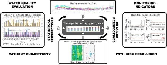
:Unlike developed countries, China has a nationally unified water environment standard and a specific watershed protection bureau to perform water quality evaluation. It is a major challenge to assess the water quality of a large watershed at a wide spatial scale and to make decisions in a scientific way. In 2016, weekly and real-time data for four monitoring indicators (pH, dissolved oxygen, permanganate index, and ammonia nitrogen) were collected at 21 surface water sections (sites) of the Yangtze River Basin, China. Results showed that one site had a relatively low Site Water Quality Index and was polluted for 12 weeks meanwhile. By using expectation-maximization clustering and hierarchical clustering algorithms, the 21 sites were classified. Variable spatiotemporal distribution characteristics for water quality and pollutants were found; some sites exhibited similar water quality variations on the weekly scale, but had different yearly grades. The results revealed polluted water quality for short periods and abrupt anomalies, which imply potential pollution sources and negative effects on water ecosystems. Potential spatio-temporal water quality characteristics, explored by machine learning methods and evidenced by time series and statistical models, could be applied in environmental decision support systems to make watershed management more objective, reliable, and powerful.
1. Introduction
Water quality evaluation is commonly based on water environment standards (WESs). In developed countries such as the United States, member states of the European Union, Australia, and Japan, the local WESs in specific states or territories are based on a national unified Water Quality Criteria (WQC). China, however, has a nationally unified WES, but without WQC [1,2]. Moreover, in developed countries, water quality assessment is enforced by local government in specific states or territories [1,3], while, in China, water quality evaluation is performed by a specific watershed protection bureau [4,5]. An example is the Yangtze River Water Resources Protection Bureau, which is responsible for a large river basin that extends across almost the entire width of the country. Due to the way water quality management is organized in China, it is a difficult challenge for the central government of China to assess the water quality on a large spatial scale and to make decisions in a scientific manner.
Various research methods have been used for water quality evaluation; most are based on water quality models and specific software with complicated calculations and diverse indices [6,7,8,9,10,11]. The objectives of these methods are to predict contaminant flux, concentration, and yield in streams, and to evaluate alternative hypotheses regarding important contaminant sources and watershed properties that control transport over large spatial scales. However, there is no unified model available for the Chinese government to make decisions regarding large watershed management [12]. Local governments have a variety of environmental models that they can choose from, and may select diverse models that do not allow meaningful comparisons with the results of models chosen in other areas [13]. Even in the same area, different departments of the same local government use different models with diverse data to assess the water quality of the same river basin, resulting in a huge amount of variability in the water quality evaluation reports, which often fail to reach the same conclusion [3,4].
Thanks to the increased collection and use of data, data-driven approaches have been playing an increasingly important role in water management [14]. Statistical and numerical models enable environmental decision support systems (EDSS) to be more reliable and powerful in coping with real-world environmental systems [15]. Real-time data are widely used in urban water management and by water utilities in developed countries [16,17,18,19,20], but rarely in rural watershed management, especially in large watershed management [21,22]. In China, the rapidly growing economy and population is generating widely distributed polluted surface water throughout the country. Thus, there is an increasing need for online data for large watershed management to meet the objectives of early warning monitoring of surface water quality, and for monitoring and control of total pollutant discharge of pollution sources [23]. Online monitoring stations with automatic analyzers for water quality have been increasingly used across China [3]. The real-time data contain four main indicators for water quality assessment: pH, dissolved oxygen (DO), permanganate index (CODMn), and ammonia nitrogen (NH3–N). The most important parameters affecting the health of aquatic ecosystems, fish mortality, odors, and other aesthetic qualities of surface waters are pH, DO, and ammonia [24]. The permanganate index is a convenient and quick measure of the chemical oxygen demand (COD). The index indicates the amount of oxygen consumed when a substance in water is oxidized by a strong chemical oxidant and is applicable to the determination of organic pollution in surface water [25,26,27].
Cluster algorithms are proven machine learning models which have been broadly used, from gene expression data in biology to stock market analysis in finance, but rarely applied in water environment management because of a lack of data [28]. Hierarchical agglomerative cluster analysis has been used to analyze high-dimensional data [29,30]. The expectation-maximization clustering algorithm can be effectively used to analyze low-dimensional data, especially when the only available data for training a probabilistic model are incomplete [31,32]. Therefore, the present study used weekly and real-time monitoring data for four indicators (pH, DO, CODMn, and NH3–N) from 21 sites of the national monitoring program of the Yangtze River Basin (YRB) collected during 2016. The Site Water Quality Index (SWQI), hierarchical clustering, and expectation-maximization clustering algorithms and time-series analyses, were used to: (a) Rank the water quality of sites, (b) classify the spatiotemporal distribution characteristics of the water quality of sites, (c) explore the spatiotemporal variation characteristics of the pollutants, and (d) discover short-period polluted conditions and abrupt abnormal events. The aims of the study were to develop numeric methods with water quality data monitoring on different time scales and to make watershed management more objective, reliable, and powerful.
2. Material and Methods
2.1. Study Area and Monitoring Sites
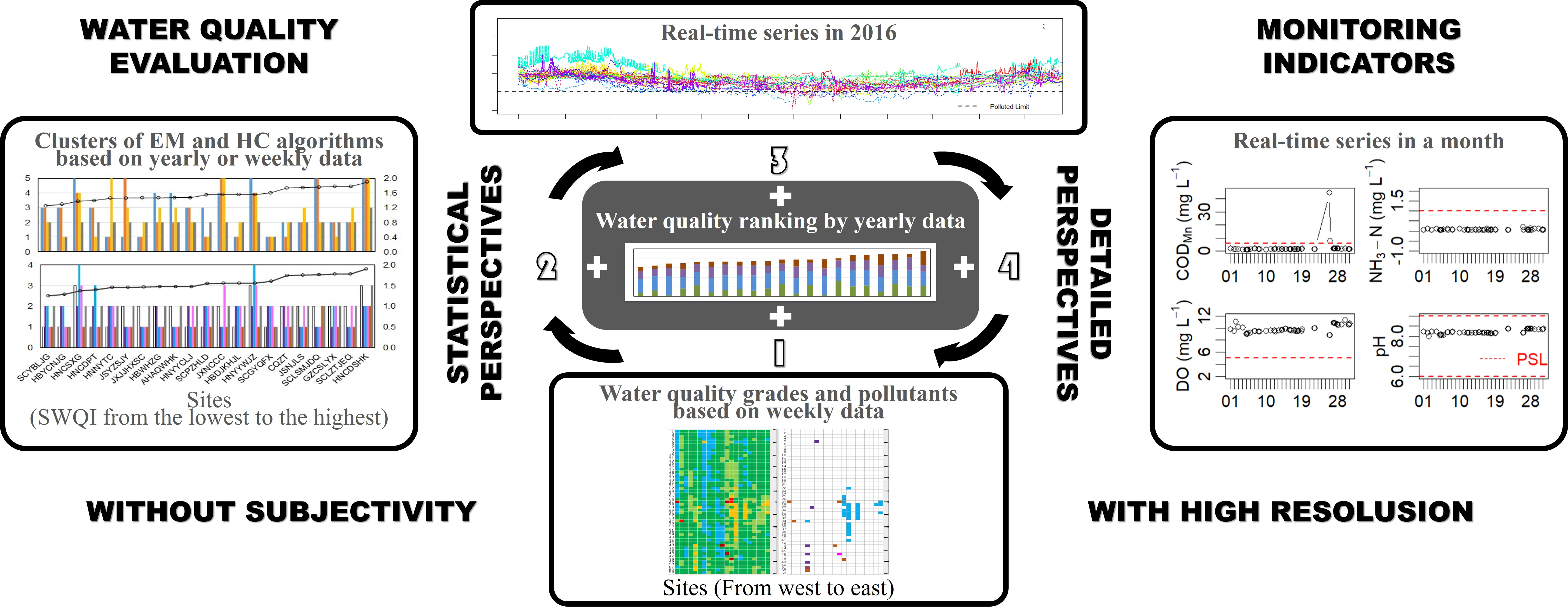
The Yangtze River, which is 6380 km long, is the longest river in Asia and the third-longest in the world. The river flows entirely within one country, drains one-fifth of the land area of the People’s Republic of China and its river basin is home to nearly one-third of the country’s population [33,34]. In 2014, China made the development of the Yangtze River Economic Belt a national strategy. The economic belt, which accounts for more than 40 percent of both the national population and GDP, was built stretching from Southwest China’s Yunnan province to Shanghai in the east and was expected to boost development in riverside regions and provide new growth stimuli for China’s slowing economy and, meanwhile, placed environmental protection and restoration as a paramount task [35,36]. The Yangtze originates from the Tuotuo on the southwestern slopes of the snow-draped Geladandong Mountains in the Tanggula Mountains on the Tibetan Plateau at about 6000 m elevation (33°28′ N, 91°08′ E). The Yangtze flows west to east across three major morphological surfaces in China into the East China Sea, with the main river past the 11 provinces (alternatively, autonomous regions or municipalities) of Qinghai, Tibet, Yunnan, Sichuan, Chongqing, Hubei, Hunan, Jiangxi, Anhui, Jiangsu, and Shanghai, and with the tributaries past the eight provinces (or autonomous regions) of Gansu, Shaanxi, Guizhou, Henan, Guangxi, Guangdong, Fujian, and Zhejiang. The Yangtze drains a basin of about 1.80 million km2 ranging from 24°30′ N to 35°45′ N of an about 1000-kilometer length (from south to north) and from 96°33′ E to 122°25′ E of an over 3000-kilometer length (from west to east) [33].
There are 21 surface water sections (sites) with real-time monitoring systems under the national monitoring program in the Yangtze River Basin (YRB) (see Figure 1). These sites are mainly on the main river of the YRB, located in the nine provinces (or municipalities) of Sichuan (five SC sites), Chongqing (one CQ site), Guizhou (one GZ site), Hunan (five HuN sites), Hubei (three HB sites), Henan (one HeN site), Jiangxi (two JX sites), Anhui (one AH site), and Jiangsu (two JS sites), and in the thirteen tributaries of the YRB. From west to east (according to the longitudes of the sites), the 21 sites were coded as followed (Table 1): Site SC1, Site SC2, Site SC3, Site SC4, Site GZ1, Site CQ1, Site SC5, Site HB1, Site HB2, Site HeN1, Site HuN1, Site HuN2, Site HuN3, Site HuN4, Site HuN5, Site HB3, Site JX1, Site JX2, Site AH1, Site JS1, and Site JS2. The first seven sites are located in the upper reaches of the YRB, and the last three are located in the lower reaches of the YRB. The others are located in the middle reaches of the YRB, except Site HB1, located at the exit of the Three Gorges Reservoir, where the Three Gorges Dam, the world’s largest power station in terms of installed capacity (22,500 MW) and whose construction was completed in 2009 [37], is located.
2.2. Monitoring Methods and Data Sources
Weekly data and real-time data of monitoring indicators at the 21 sites of the YRB in 2016 came from China National Environmental Monitoring Centre. Weekly data were collected from the weekly reports on automatic monitoring data of national water quality (http://www.cnemc.cn/sssj/szzdjczb/) and real-time data were collected from the publishing system of real-time automatic monitoring data of national surface water quality (http://58.68.130.147/#) [38,39]. The monitoring indicators included pH, dissolved oxygen (DO), permanganate index (CODMn), and ammonia nitrogen (NH3–N). The monitoring frequency of one weekly sample is a week and the monitoring frequency of one real-time sample is four hours.
2.3. Water Quality Indices and Statistical Analysis
2.3.1. Water Quality of SWQI and Grades
City Water Quality Index (CWQI), quoted from Technical Regulations of Urban Surface Water Quality Ranking (on trial) (MEP General Office [2017] No.51) [40], is built to reflect the condition of the whole city surface water environment. The method is universal, operable, and comparable [41]. The CWQI was brought to assess and rank site water quality, and named as the Site Water Quality Index (SWQI). The yearly average values of the monitoring indicators were calculated first, then SWQI (i) (i for a specific monitoring indicator) and finally SWQI of a specific site was reached. The calculation methods are as follows:
As for the monitoring indicators such as permanganate index and ammonia nitrogen, SWQI (i) is given by
where C (i) is the yearly average value of the monitoring indicator i, Cs (i) is the polluted standard limit of Level III of the monitoring indicator I (No. GB3838-2002, Table 2) [2].
SWQI (i) = C (i)/Cs (i)
For DO, SWQI (i) is given by
where C (DO) is the yearly average value of DO concentration, and Cs (DO) is the polluted standard limit of Level III of DO (No. GB3838-2002, Table 2) [2].
SWQI (DO) = Cs (DO)/C (DO)
For pH, when pH ≤ 7, SWQI (i) is given by
SWQI (pH) = (7.0 − pH)/(7.0 − pHsd)
When pH > 7, SWQI (i) is given by
where pHsd is the lower standard limit of the normal water quality and pHsu is the higher standard limit of the normal water quality (No. GB3838-2002, Table 2) [2].
SWQI (pH) = (pH − 7.0)/(pHsu − 7.0)
Based on the SWQIs above, SWQI of a specific site is given by
where SWQI (i) is the SWQI of the monitoring indicator i, and n is the total number of the monitoring indicators. Water quality of the 21 YRB sites was ranked by SWQI, where higher SWQI meant worse water quality and ranked lower.
The yearly and weekly water quality grades of the 21 sites were determined by the Environmental Quality Evaluation Methods for Surface Water in China (on trial) (MEP General Office [2011] No.22) [42] with single indices calculated by the monitoring indicators, combined with the standard limits and water quality levels in the No. GB3838-2002 document (Table 2), the comprehensive water quality of one site in one specific period was defined by the worst quality level of the four indicators and graded into six levels: Grade Ⅰ, Grade Ⅱ, Grade Ⅲ, Grade Ⅳ, Grade Ⅴ, and Grade inferior to Ⅴ. Water quality of one specific period at one site with the water level worse than the Ⅲ level (also PSL) is identified as being polluted in that period at that site, i.e. one polluted week of the site. The ratio of unpolluted weeks at one site was calculated by (100% - the ratio of polluted weeks) at that site. The index/indices with values in the ranges of the polluted conditions were defined as the main pollutant index/indices.
2.3.2. Statistical Analysis
Coefficient of Variation
The coefficient of variation (CV) is a normalized measure of the uncertainty of these indicator values and calculated in a given year as the standard error of the indicator [StdErr (Indicator)] divided by the indicator value (observed indicator value) [43]:
As for the four monitoring indicators, the yearly CV (i) is given by
where StdErr (i) is the standard error of the monitoring indicator i of weekly values, and C (i) is the yearly average value of the monitoring indicator i.
CV (i) = StdErr (i)/C (i)
Clustering Analyses
In this study, hierarchical agglomerative cluster (HC) analysis was performed on the normalized data set by Ward’s method, using squared Euclidean distances as a measure of similarity [44]. Ward’s method looks for clusters in multivariate Euclidean space, the reference space in multivariate ordination methods and, particularly, in principal component analysis. The number of clusters, K, of the HC algorithm was determined by the multi-index method in which 30 indices determine the number of clusters in a data set and the best clustering scheme from different results is also offered [45]. The expectation–maximization (EM) clustering algorithm, an iterative method to find maximum likelihood or maximum a posteriori (MAP) estimates of parameters in statistical models and, depending on unobserved latent variables [32,46], was chosen to classify the water quality of the 21 sites in YRB with the Bayesian Information Criterion (BIC) selected as the model identification criteria [32]. Classification of the 21 sites in the YRB had done by three EM algorithms and five HC algorithms (Table 3). The EM_Class_Y classifications represented the clustering results from the EM algorithm with data of the yearly average values of the four monitoring indicators (EM_Y Method). The EM_Class_R classifications represented the clustering results from the EM algorithm, based on data of yearly SWQI (i)s and ratios of unpolluted weeks (EM_R Method). The EM_Class_CVR classifications represented the clustering results from the EM algorithm, based on data of ratios of unpolluted weeks and CVs of weekly data of the monitoring indicators (EM_CVR Method). The HC_Class_Y classifications represented the results from the HC algorithm, based on data of the yearly average values of the four monitoring indicators (HC_Y Method). The HC_Class_pH classifications represented the clustering results from the HC algorithm, based on data of weekly average values of pH (HC_pH Method). The HC_Class_DO classifications represented the clustering results from the HC algorithm, based on data of weekly average values of DO (HC_DO Method). The HC_Class_COD classifications represented the clustering results from the HC algorithm, based on data of weekly average values of CODMn (HC_COD Method). The HC_Class_NH classifications represented the clustering results from the HC algorithm, based on data of weekly average values of NH3-N (HC_NH).
Correlation Analyses
The temporal relationship between the weekly means and daily means of the four indicators at different sites were performed by Spearman Correlation. Significance levels are reported as non-significant (no signs, p > 0.05) or significant (*, p < 0.05; **, p < 0.01; ***, p < 0.001).
The statistical analyses above were done by the Microsoft Excel 2016 and the clustering models were implemented by the RStudio (Version 1.0.153 with R 3.4.1).
3. Results
3.1. Water Quality Indices and SWQI Ranking of Sites in the YRB
According to government document No. GB3838-2002, the pollution standard limit of Level Ⅲ (PSL (Ⅲ)) for pH, DO, CODMn, and NH3–N are 6–9, 5, 6, and 1, respectively. In 2016, the yearly means of the four monitoring indicators of the 21 sites in 2016 all met the pollution standards (Table 4). However, the CODMn maximums for the weekly means for Sites CQ1, GZ1, and SC5 exceeded the PSL of 6 mg L−1 and were 6.5, 6.8, and 8.3 mg L−1, respectively. The maximums of the NH3–N weekly means for six sites exceeded the PSL of 1 mg L−1; the highest value was 2.88 mg L−1 at Site HuN1. The minimums of the DO weekly means for Sites HuN3, HuN4, HB3, JS2, GZ1, and JS1 fell below the PSL of 5 mg L−1; the values were 2.69, 3.82, 4.08, 4.34, 4.59, and 4.75 mg L−1, respectively.
The coefficient of variations (CVs) of the weekly values of NH3-N, CODMn, DO, and pH ranged between 0.23–1.81, 0.13–0.64, 0.09–0.26, and 0.01–0.10, respectively. The maximum CV was CV (NH3–N) for Site SC1. The maximum CV (CODMn) weekly values were at Site GZ1. The CV (DO)s and CV (pH)s were relatively low (Table 4).
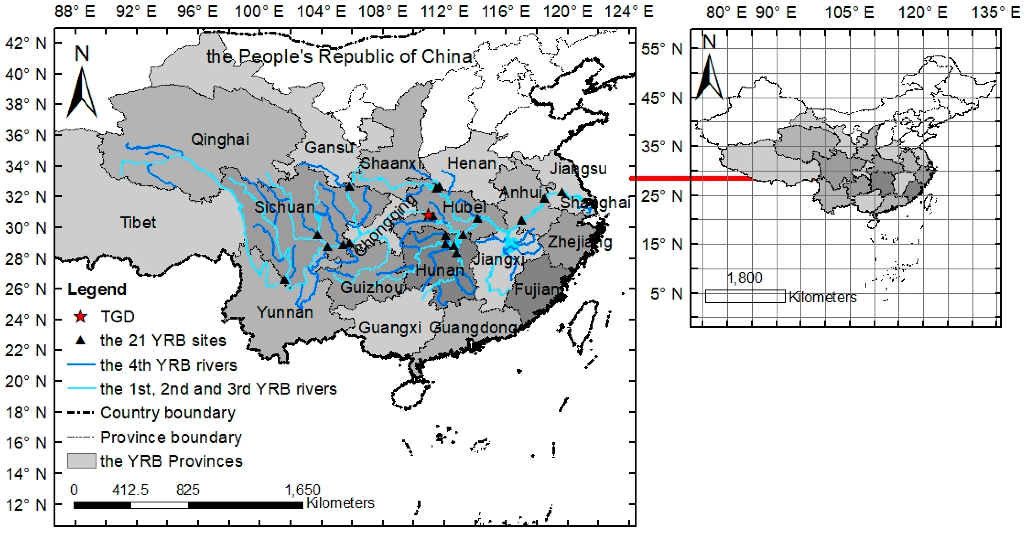
Sites HuN2, SC4, and GZ1 had the highest SWQIs (Figure 2), while Sites HuN4, HB1, and SC3 had the lowest SWQIs. Moreover, Sites SC5, HeN1, and JX1 had the lowest SWQI (NH3–N)s; Sites HuN2, SC1, and SC5 had the lowest SWQI (CODMn)s; and Sites HuN1, HeN1, and SC1 had the lowest SWQI (DO)s.
3.2. Water Quality Grades and Main Pollutants of the YRB Sites
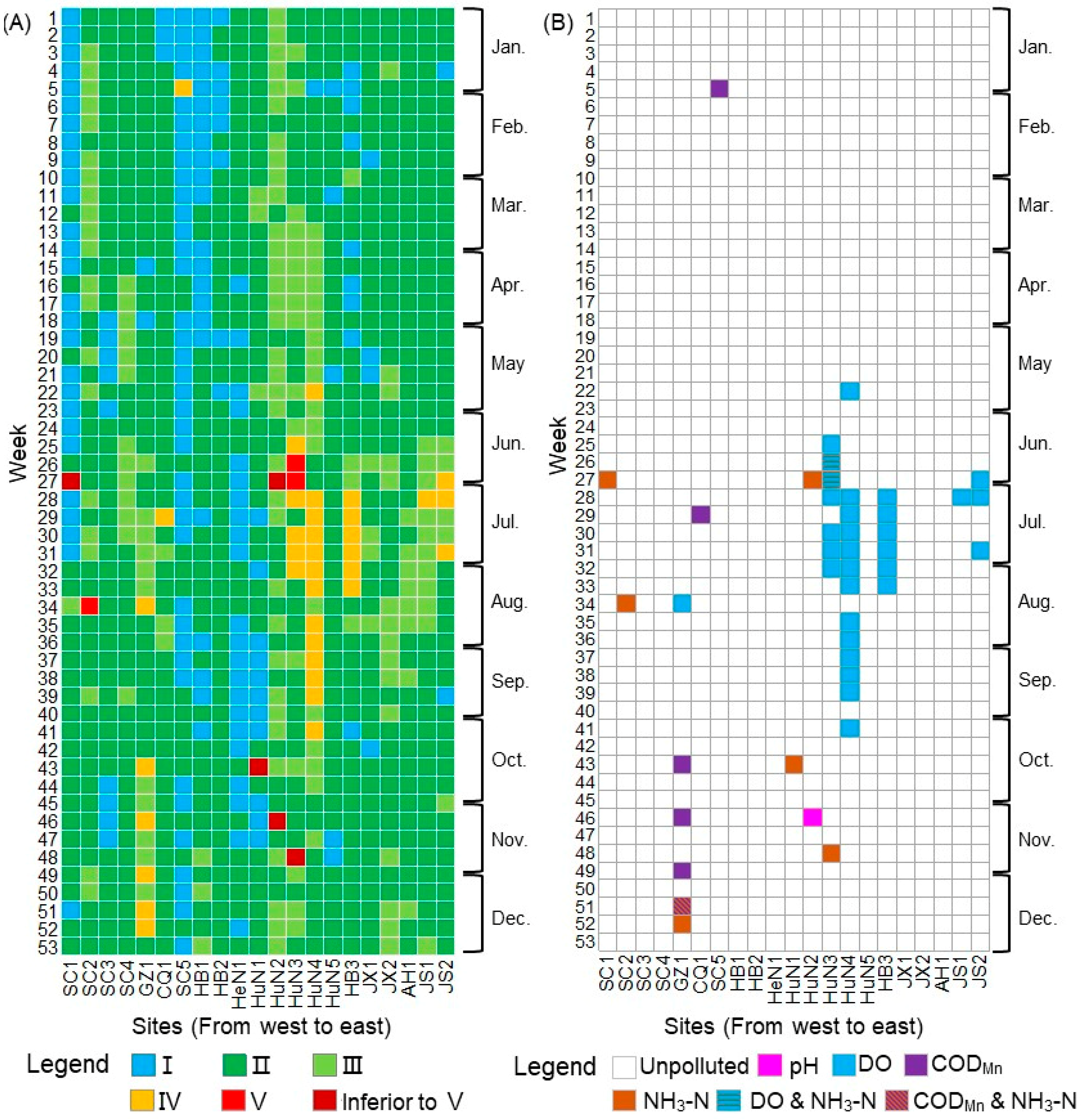
According to the weekly grade assessment results, the Sichuan (SC) sites had more weeks with good water quality than the Hunan (HuN) sites (Figure 3). In 2016, there was only one week with water pollution at the SC sites, while there was about one quarter of the 53 weeks with polluted water at the HuN sites. DO was the main pollutant index at the two HuN sites (Site HuN3 and Site HuN4), the two Jiangsu sites (Site JS1 and Site JS2), and Site HB3 in Hubei Province. In the second half of 2016, pollution by ammonia nitrogen occasionally occurred in some sites in Sichuan, Guizhou, and Hunan provinces. The permanganate index was the main pollutant index at Site GZ1 from the 43rd to the 51st weeks, at Site CQ1 in the 29th week, and at Site SC5 in the 5th week.
3.3. Clustering Analysis of Water Quality at the YRB Sites
3.3.1. Clustering Algorithms vs Single Indices Based on Yearly Monitoring Data
HC and EM clustering, based on yearly average values of the four monitoring indicators, generated different classification results for the 21 sites in the YRB.
HC clustering classified the sites into three classes: HC1, HC2, and HC3 (Figure 4). The HC1 class included four sites in Hunan Province, three sites in Sichuan Province, and one site in Hubei Province. The HC2 class included ten sites in the eight provinces, across the entire geographical span of the YRB. The HC3 class included Sites JS1, CQ1, and SC4. When compared with the grade results from the single-index evaluation methods in the government literature, the Grade I sites belonged to the HC1 class; Grade II were associated with all three HC classes; and Grade III sites belonged to the HC3 class.
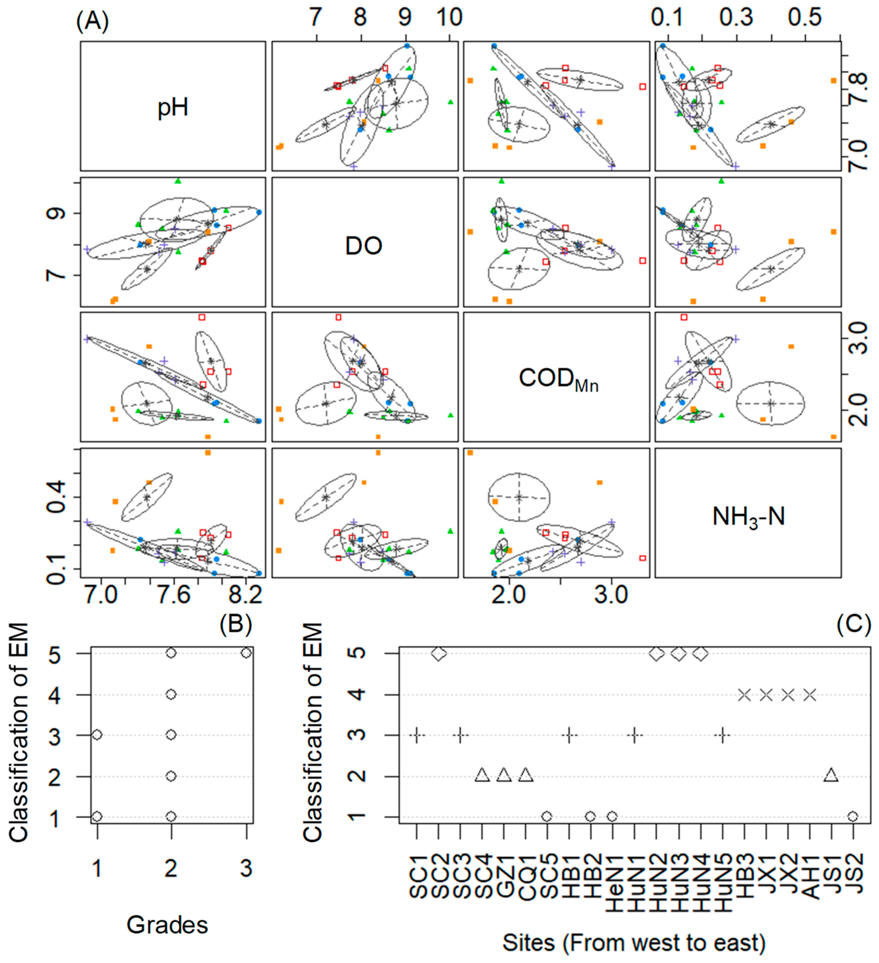
Based on the EM clustering results (Figure 5), the 21 sites were classified into five EM algorithm classes: EM1, EM2, EM3, EM4, and EM5. Compared with the grade results from the single-index evaluation methods in the government literature, the EM1 class contained a Grade 1 site (Site SC5) and Grade II sites (Sites JX1, HB2, HeN1, and JS2). The EM2 sites (Sites CQ1, JS1, GZ1, and SC4) and the EM4 sites (Sites AH1 and JX2) belonged to Grade II. The EM5 class had relatively high annual averages of NH3-N and relatively low annual averages of DO, and contained Grade II sites (Sites SC2, HB3, HuN4, and HuN3) and one Grade III site (HuN2).
Overall, the EM3 sites belonged to the HC1 class. The EM2 and EM4 sites belonged to the HC2 class. Some EM1 sites belonged to the HC1 class (Sites SC5, HB2, and HeN1) and some EM1 sites belonged to the HC2 class (Sites JX1 and JS2). The HC3 sites belonged to the EM5 class (Sites HuN2, HuN3, and HuN4).
3.3.2. Pollution Characteristics Using EM Clustering for Yearly and Weekly Monitoring Data
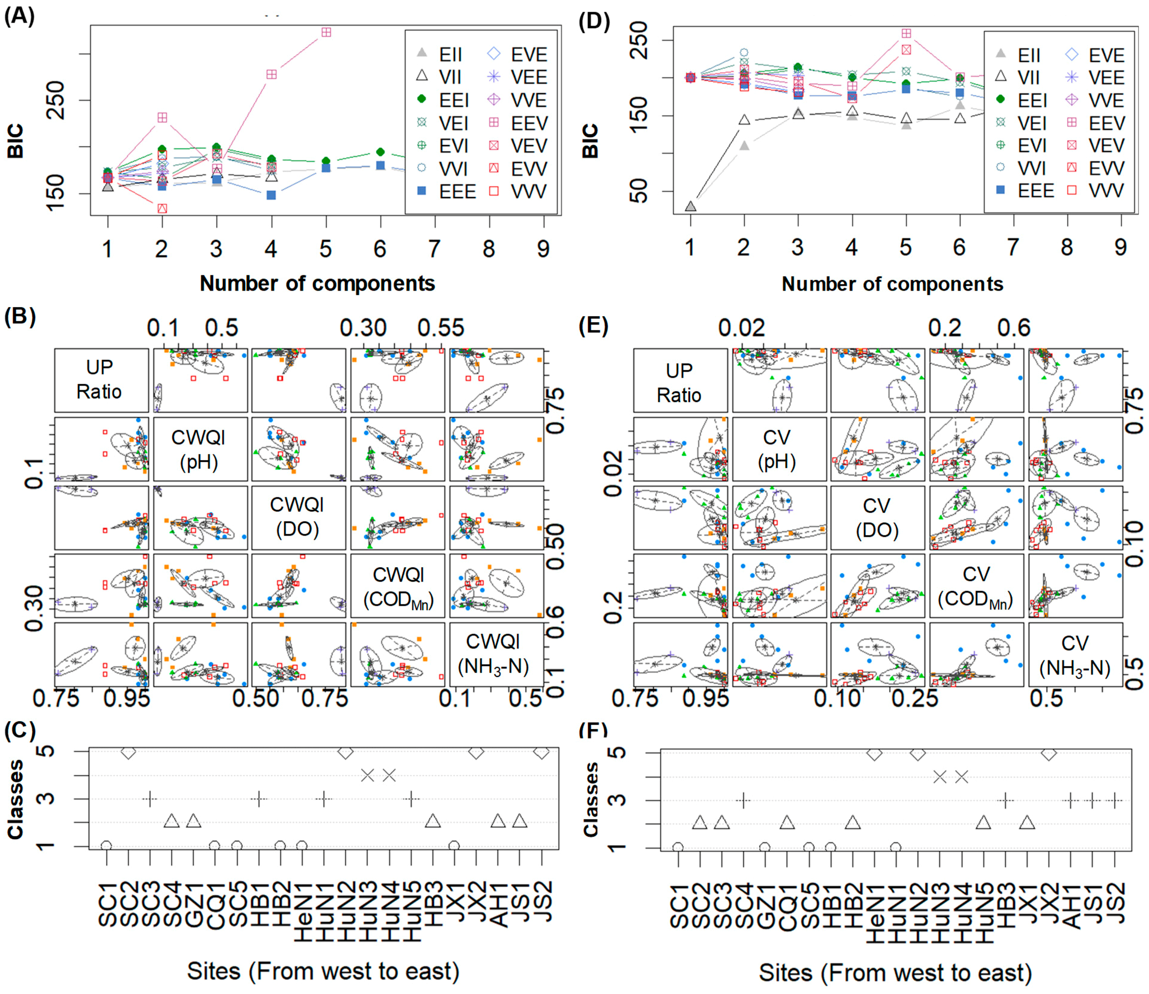
The yearly SWQI(i)s of the four monitoring indicators and ratios of unpolluted weeks were chosen as the input data for EM clustering (see Figure 6A–C). The ellipsoidal equal volume and shape model (EEV) with five components (Mclust EEV (K = 5) model) was the best model, based on the BIC criterion. This model had the largest BIC value (323.3296) and log-likelihood (289.5348). According to the Mclust EEV (K = 5) model, six sites in four provinces were classified in the EM1 class, five sites of five provinces were classified in the EM2 class, four sites of three provinces were classified in the EM3 class, two HuN sites were classified in the EM4 class, and four sites of four provinces were classified in the EM5 class. According to the Mclust EEV (K = 5) model, the EM1 class represented a relatively high ratio of unpolluted weeks and a relative large SWQI (pH) and small SWQI (DO), SWQI (CODMn) and SWQI (NH3–N). The EM2 class represented a relatively high ratio of unpolluted weeks and a relatively small SWQI (NH3–N) and medium-level of SWQI (DO), SWQI (pH) and SWQI (CODMn). The EM3 class represented a relatively high ratio of unpolluted weeks and a relatively small SWQI (DO), SWQI (CODMn), and SWQI (NH3–N). The EM4 class represented a low ratio of unpolluted weeks and a relatively large SWQI (DO) and low SWQI (pH) and SWQI (CODMn). The EM5 class represented a relative high ratio of unpolluted weeks and a relatively large SWQI (CODMn) and SWQI (NH3–N).
The yearly CV (i)s of the four monitoring indicators and ratios of unpolluted weeks were chosen as the input data of EM clustering (Figure 6D–F). The ellipsoidal equal volume and shape model (EEV) with five components (Mclust EEV (K = 5) model) was the best model based on the BIC criterion, with the largest BIC value of 259.2801 and log-likelihood of 257.51. According to the Mclust EEV (K = 5) model, five sites of four provinces were classified into the EM1 class, six sites of five provinces were classified into EM2 class, five sites of four provinces were classified into EM3 class, two HuN sites were classified into EM4 class, and three sites (Sites HeN1, HuN2, and JX2) of Hunan and Jiangxi provinces were classified in the EM5 class. According to the Mclust EEV (K = 5) model, the EM1 class represented a relatively high ratio of unpolluted weeks and relatively large CV (NH3–N)s. The EM2 class represented a relatively high ratio of unpolluted weeks and relatively small CVs of the four indices. The EM3 class represented a relatively high ratio of unpolluted weeks and relatively large CV (DO)s The EM4 class represented a low ratio of unpolluted weeks and relatively large CV (DO)s. The EM5 class represented a relatively high ratio of unpolluted weeks and relatively large CV (pH)s.
When the classification results from three EM clustering algorithms (Figure 7) are compared with the grade and SWQI results (see Section 3.3.1), the site with the highest SWQI and the highest grade is the same (Site HuN2) and has three EM classes (EM_Class_Y 5, EM_Class_R 5, and EM_Class_CVR 5). Site SC2 had the same EM_Class_Y and EM_Class_R as Site HuN2, but had different grades. Similar results occurred at Sites JX2 and HuN2, clustered in the same EM_Class_R and EM_Class_CVR yet with different grades, and at Sites JS2 and HuN2 clustered in the same EM_Class_R yet with different grades. Sites HB3 and AH1 shared the same classes of the three EM clustering models (EM_Class_Y 4 EM_Class_R 2, EM_Class_CVR 3) also with the same water quality grade (Grade II) and close SWQIs. The same qualities occurred at the two HuN sites (Sites HuN4 and HuN3) on the middle reaches of the YRB, which classified in the same clusters of the three EM clustering models, also at Sites JX1 and HB2, Sites SC3 and HuN5, Sites JS1 and SC4. Sites HB1 and HuN1 shared the EM_Class_Y 3, EM_Class_R 3 and EM_Class_CVR 1, but had different grades (Grade I and Grade II, separately). Sites HeN1 and SC5 both belonged to the EM_Class_Y 1 and EM_Class_R 1, but were in different classes of the EM_Class_CVR model and different grades.
3.3.3. Temporal Distribution Characteristics Using HC Clustering and Weekly Monitoring Data
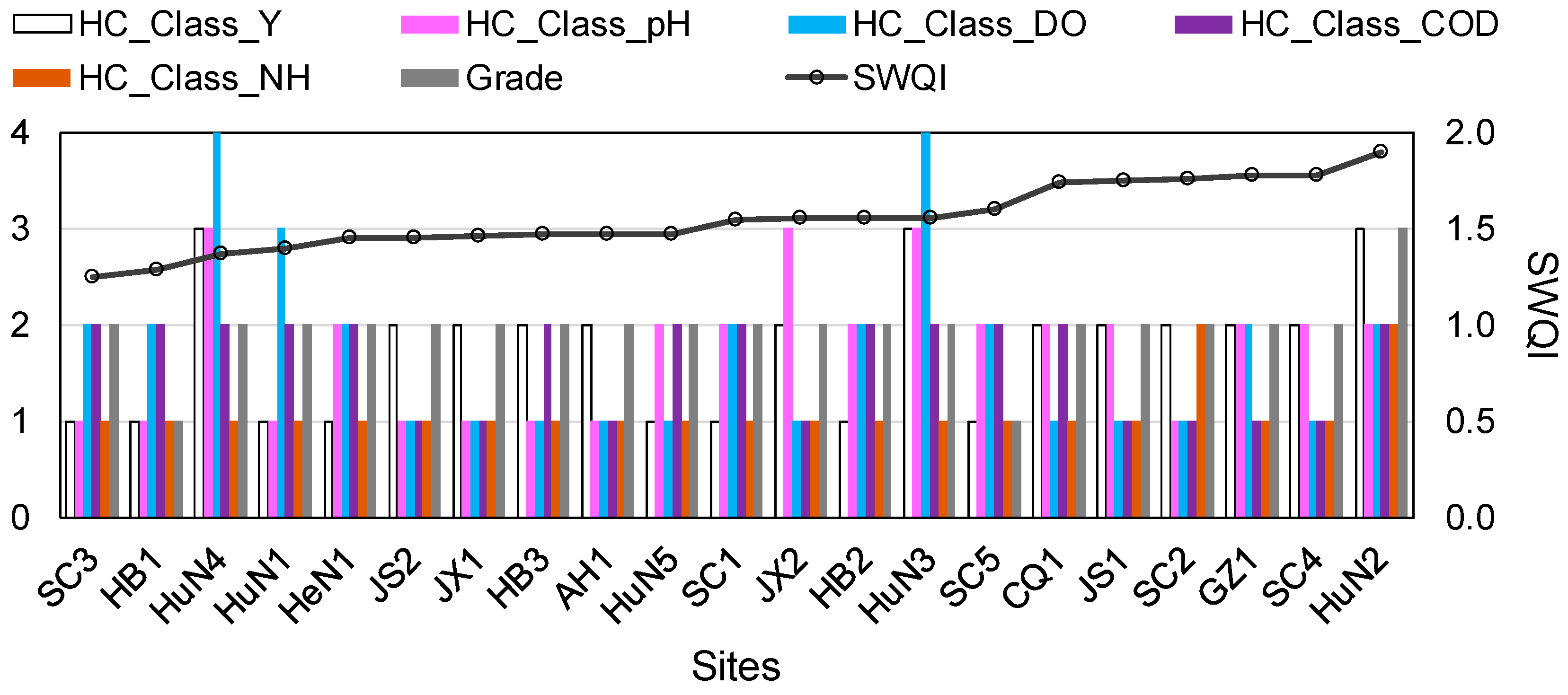
By different hierarchical clustering algorithms, the 21 sites were classified into three HC_Y clusters, three HC_Class_pH clusters, four HC_Class_DO clusters, two HC_Class_COD clusters and two HC_Class_NH clusters (Figure 8). When compared with the classification results from the five EM clustering algorithms with the grade and SWQI results mentioned earlier, the two HuN sites (Sites HuN4 and HuN3) had the same classes for the five hierarchical algorithms with the same grade. Site HuN2 had the same classes for the HC_Class_Y and HC_Class_COD models as Sites HuN3 and HuN4 but had different classes for the other three models. Sites HeN1, SC1, HB2, and Site SC5 had the same classes of the five HC models with the same water quality grade, except for Site SC5, which was Grade Ӏ. Sites SC3 and HB1 had the same classes for the five HC models and similar SWQIs with different grades, Grade Ӏ and Grade Ⅱ respectively. Sites HuN1 and HuN5 belonged to the same HC_Class_Y, HC_Class_COD and HC_Class_NH but had different classes for the HC_Class_DO and HC_Class_pH models. Sites JS2, JX1, and Site AH1 had the same classes for the five HC models with the same grades, as did Sites JS1 and SC4. Sites HB3 and CQ1 belonged to different classes of the HC_Class_pH model but shared the same classes for the other four HC models and shared the same grade. Sites JX2, SC2, and GZ1 shared the same classes for the HC_Class_Y and HC_Class_COD models but had different classes of the other HC models.
3.4. Real-Time Series Analyses of the YRB Sites
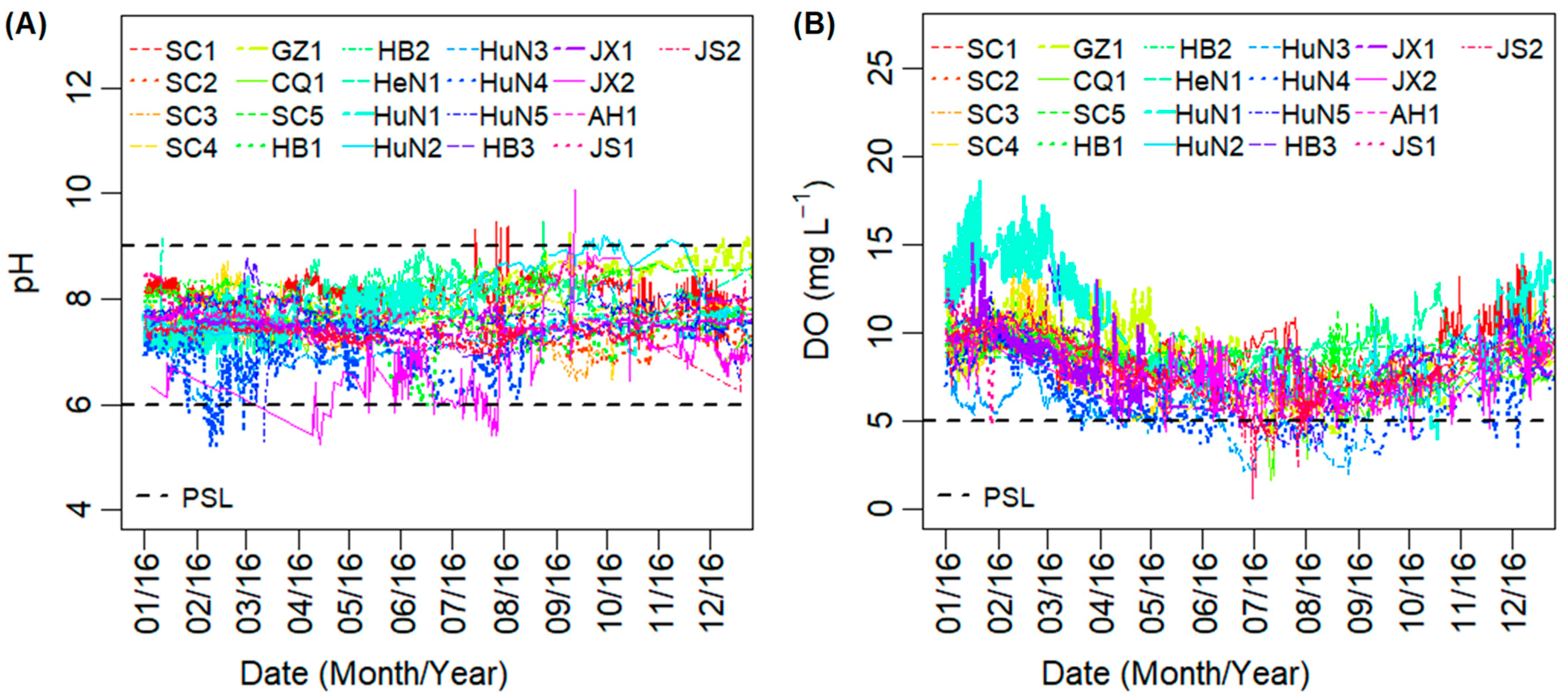
The pH time series indicated the presence of acid-polluted water at Sites HuN4 and HuN3 in February 2016 and Site JX2 from April to July of 2016. Alkali-polluted water was mainly detected at Site GZ1 in December 2016, at Site HuN2 in September and October of 2016 and at Site SC1 in July and August of 2016 (Figure 9A).
The DO time series indicated that in June, July, and August of 2016 there were monitoring values below the lower limit of Grade Ⅴ of 2 mg L−1 at Sites CQ1, HuN3, and Site JS2. At Site HuN4, DO concentrations below the PSL(Ⅲ) of 5 mg L−1 occurred frequently from March to December of 2016 (Figure 9B). Overall, there were the similar pollution and fluctuation characteristics of DO between Site HuN3 and Site HuN4.
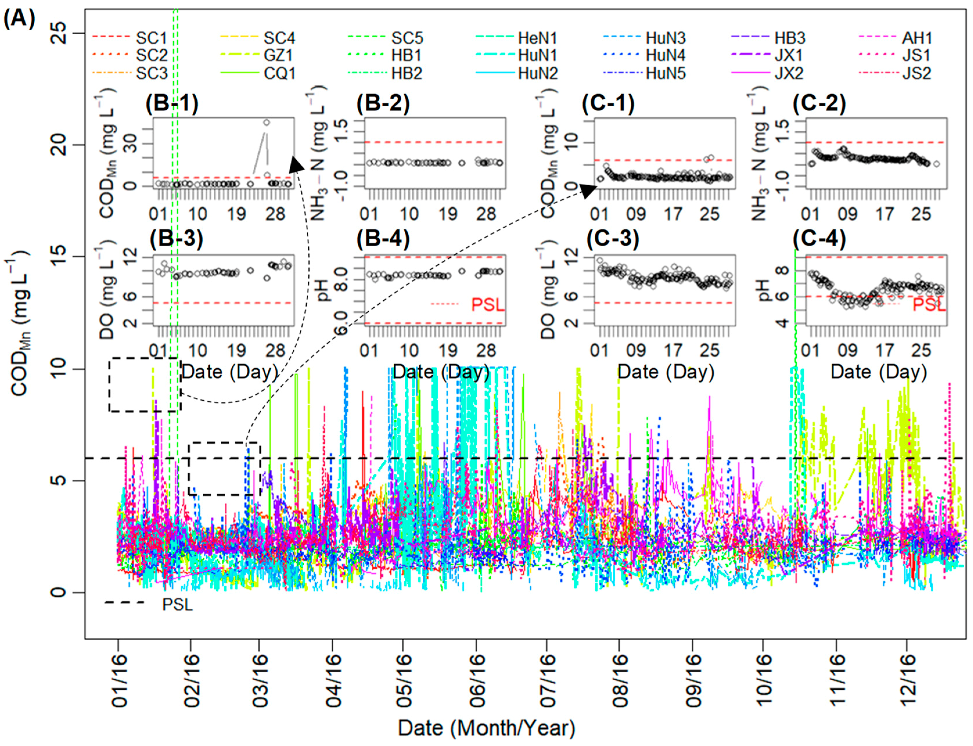
At two of the Hunan Province sites (Sites HuN1 and HuN3), water pollution, indicated by CODMn values in excess of 6 mg L−1, occurred frequently from April to June of 2016. There were monitoring values over 6 mg L−1 at Site GZ1 from October to December of 2016. There were occasional monitoring values over 6 mg L−1 at the two Sichuan Province sites (SC2 and SC4) (Figure 10A). Site SC5 had only one CODMn value over 40 mg L−1 on 26 January, which caused the weekly average to be higher than the Grade V limit of 15 mg L−1 (see Section 3.2) and much higher than the pollution limit of 6 mg L−1. The other indicators indicated no pollution at Site SC5 (Figure 10B). During February 2016, at Site HuN4, two monitoring values of CODMn exceeded the PSL (on 24 and 25 February), and 34 monitoring samples had a pH lower than 6 (from 7 to 16 February) (Figure 10C).
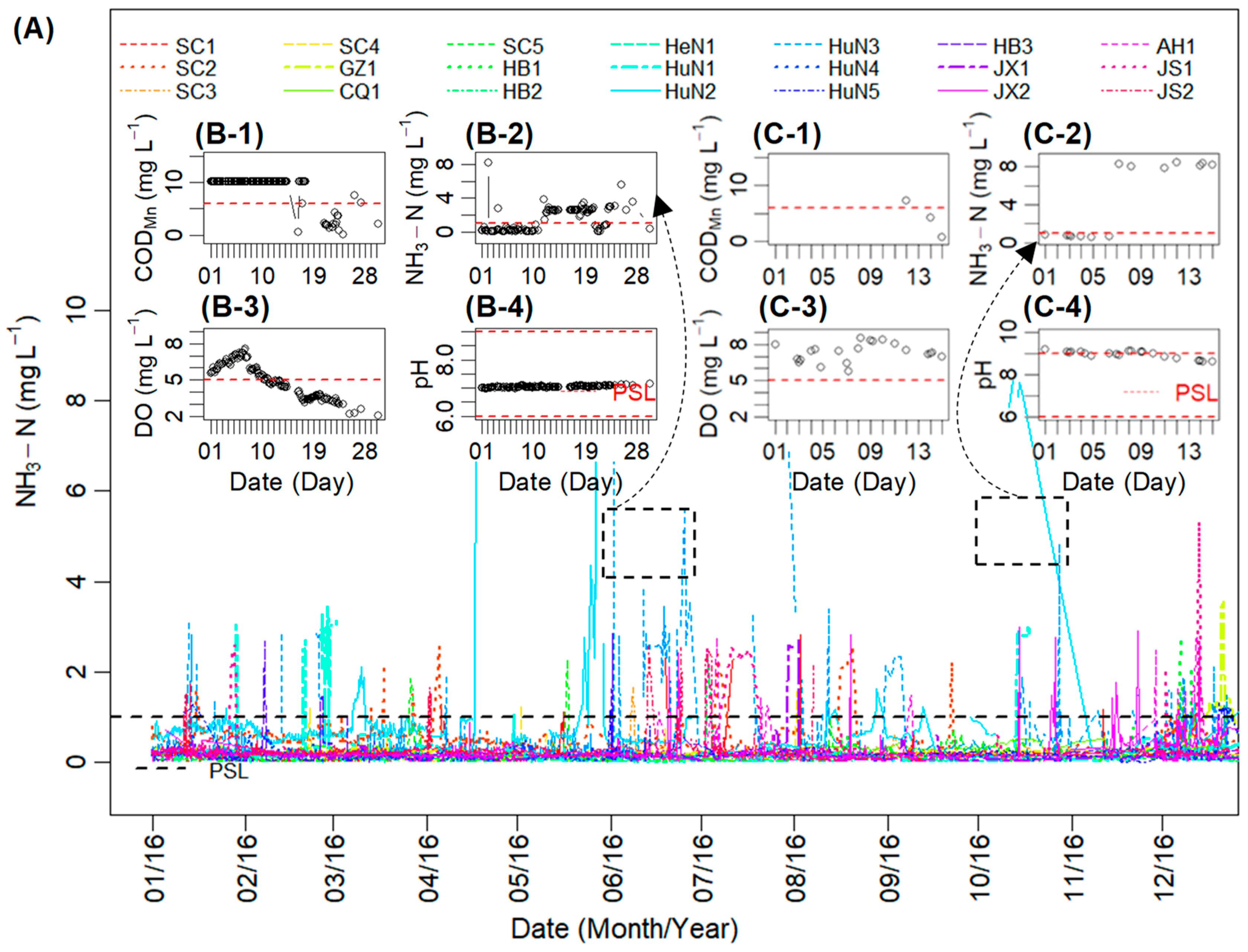
Nearly half of the monitoring samples for June 2016 at Site HuN3 exceeded the Grade V limit of 2 mg L−1, and some monitoring samples had high NH3–N concentrations of over 1 mg L−1 throughout the year at this site, except for May. NH3–N values exceeded the polluted limit of 1 mg L−1 in most of the months, except for February and November. In December of 2016, there were ten sites with high NH3–N concentrations of over 1 mg L−1 (Figure 11A). When looked at in more detail, there were 52 monitoring samples with NH3–N concentrations above 1 mg L−1 and 66 with DO concentrations below 5 mg L−1 at Site HuN3 in June 2016; DO and NH3–N were the main indicators of polluted water quality after 11 June (see Section 3.2). The CODMn values were constant, at 10.07 mg L−1, from 1 June to 17 June, which suggests that the monitoring devices were malfunctioning (Figure 11B). In October 2016, at Site HuN2, the NH3-N concentrations exceeded 8 mg L−1 for 9 days and the pH exceeded 9 for some of the days (Figure 11C).
3.5. Temporal Correlation Analyses between Different Sites
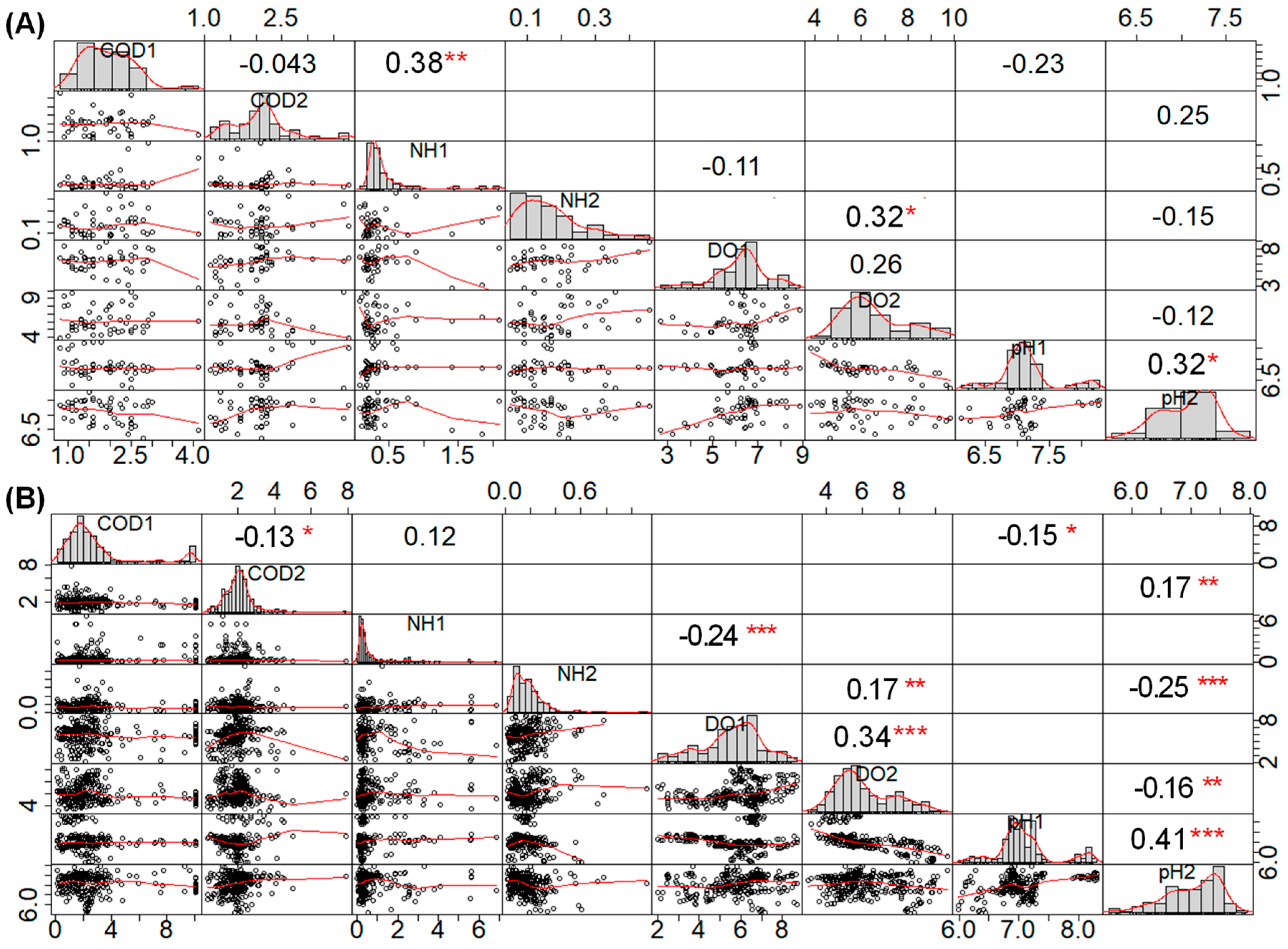
Results from Spearman Correlation analyses (Figure 12, most data were abnormally distributed) showed temporal correlations between each two of the weekly and daily means of the four indicators through 2016 at Sites HuN3 and HuN4. The pH values, in weeks, had a significantly positive correlation between Sites HuN3 and HuN4 (Spearman coefficient, 0.32; p < 0.05). CODMn and NH3–N in weeks had a significantly positive correlation at Site HuN3 (Spearman coefficient, 0.38; p < 0.01), while NH3–N and DO in weeks had a significantly positive correlation at Site HuN4 (Spearman coefficient, 0.38; p < 0.05). The four indicators in days at Sites HuN3 and HuN4 had more significant correlations between each other than those in weeks. Different from the correlation result of weekly means, DO daily means were significantly positively correlated between Sites HuN3 and HuN4 (Spearman coefficient, 0.34; p < 0.001), while CODMn daily means were significantly negatively correlated between the two sites (Spearman coefficient, −0.13; p < 0.05). NH3–N and DO daily means were significantly negatively correlated at Site HuN3 (Spearman coefficient, −0.24; p < 0.001), while they were significantly positively correlated at Site HuN4 (Spearman coefficient, 0.17; p < 0.01). The pH daily means had significantly negative correlations with DO and NH3–N daily means at Site HuN4, but had a significantly positive correlation with CODMn daily means. Different from Site HuN4, the daily means of pH had a significantly negative correlation with those of CODMn at Site HuN3.
4. Discussion
4.1. Limitation of SWQI and Yearly Data for Water Quality Evaluation
When compared with other basins in the YRB, the ratios of the river lengths meeting the Grade Ⅲ water quality were relatively low, less than 80% in the basins of the Minjiang and Tuojiang River (the upper reaches of the YRB in Sichuan Province), the Wu River (the lower reach of the YRB in Jiangxi Province), and the Taihu Lake (the lower reach of the YRB in Jiangsu Province) [4]. This agreed with the SWQI results of the SC Sites with relatively high SWQIs and relatively bad water quality, but disagreed with the SWQI results of the JX and JS sites. Overall, SWQIs calculated from yearly data did not successfully capture the true water situation throughout the year.
First, low SWQIs failed to indicate good water quality. For example, Site HuN4, ranked in the top three for SWQI, had twelve polluted weeks with a DO lower than the PSL value of 5 mg L−1; this was not captured by the yearly SWQI. Although the sites in Hunan Province (with relatively high yearly SWQIs) ranked before the sites in Sichuan Province (Figure 2), it is not reasonable to conclude that the Hunan water quality was better than the Sichuan water quality. Results from the weekly quality levels revealed that the sites in Hunan Province have worse water quality than those in Sichuan Province. This may be because the Hunan Province has fewer waste water treatment plants, and, in 2016, had smaller amounts of waste water that were treated, and smaller volumes of waste water that were recycled and reused. Thus, more waste water may have been input into the surface water [47].
Second, not all the monitoring indicators were suitable for ranking the water quality. Site HB3 had six polluted weeks when DO was identified as the main pollution index, but had a lower SWQI (DO) than Site HB1, which had no polluted weeks. This occurred because, in normal situations, DO is always supersaturated in water. The more highly supersaturated DO failed to indicate better water quality, as the DO levels were was mainly related to temperature and atmospheric factors, such as atmospheric temperature and wind speed [48,49]. Although DO supersaturation has little relationship with the polluted water quality, low concentrations of DO are associated with polluted water, and continuously low concentrations of DO in water can cause the water to have a black color and/or unpleasant odors [50]. The SWQI (pH) differences could not be used to account for pollution levels at different sites because the yearly pH means were all in the unpolluted range. Only the SWQI (i)s, calculated from monitored data, indicating polluted conditions, were meaningful for water quality ranking. If a single SWQI (i), calculated from different indicators, is used for the SWQI, it should have different weights for the different indicators.
The Report on the State of the Environment in China for 2016 concluded that the YRB had satisfactory water quality, and none of the 510 water sections in the national monitoring program failed to meet the Grade V standard [3]. However, in 2016, there were several weeks with poor water quality that failed to meet the Grade V standard at some sites in Sichuan and Hunan provinces. The main pollutant was NH3–N (Figure 3). It is suggested that the polluted weeks should be given more attention when considering potential pollution sources and the possible negative effects on water ecosystems.
4.2. The Application of Multiple Classifications and Correlations for Water Quality Evaluation
Water quality at Site HuN2 was assessed as Grade Ⅲ according to the yearly report and annual averages and was the worst site in the YRB in 2016, but belonged to the same clusters of HC_Class_Y 3 and EM_Class_Y 5 as two other HuN sites (Sites HuN3 and HuN4). Although there were only one or two weeks of polluted conditions at Sites SC2 and HuN2, they were classified in the EM5 class as Sites HuN4 and HuN3, due to of the relatively high yearly mean of ammonia nitrogen.
Unlike other clustering algorithms, the EM algorithm with the maximum likelihood method assesses the quality of a statistical model, based on the probability that it assigns to the observed data [32,51]. The 21 sites were classified into more classes by EM clustering than by HC clustering based on the annual averages of the four monitoring indicators. More than one statistical method should be used to give more perspectives of water quality, in order to explore different pollution conditions at different sites and to highlight the geographical pollution characteristics of a specific river basin.
With more polluted weeks than other sites in 2016, two sites in Hunan province (Sites HuN4 and HuN3) on the middle reaches of the YRB had the same clusters regardless of which EM or HC models were used, which were also evidenced by the real-time series analyses (see Section 3.4) and the temporal correlation analyses (see Section 3.5). This implies that they had the same polluted characteristics and low DO monitoring values, probably because of their close spatial positions and similar sources of pollution, although they were located on different tributaries of the YRB, the Xiangjiang River for Site HuN4 and the Zishui River for Site HuN3. Site SC1 (located in the upper reaches of the YRB), Site HB1 (located at the Three Gorges Dam), and Site HN1 (located in the middle reaches of the YRB) shared the same EM_Class_CVR and most weekly-data HC models. This implies that they had the same weekly water quality variations throughout 2016, although they had different yearly grades. The similar results also occurred at Site HeN1 in Henan Province and Site SC5 in Sichuan Province shared the same classes of the EM and HC models.
Machine learning methods, such as hierarchical clustering or expectation-maximization clustering algorithms, can solve the incapability of supervised classification on avalanche of data, using unsupervised approaches to extract knowledge from huge datasets [28]. The clustering results, based on real-time and weekly monitoring data of water quality, are free of subjectivity and have no need for other complex data inputs, could easily be applied to water quality evaluation. These methods would enable feasible and comparable implementations and provide scientific supports for the watershed decision-makers to assess spatiotemporal pollution characteristics and to determine the pollution sources.
4.3. Necessity of Real-time Monitoring for Water Quality Interpretation
Real-time data indicated poor water quality in terms of DO at Site CQ1 in June, July, and August of 2016, and at Site HuN4 in March and April of 2016. This poor water quality was not identified by the weekly or yearly data. Ambient dissolved oxygen concentrations lower than 4 mg L−1 within one day can harm aquatic life in freshwater [52]. Water pollution by ammonia nitrogen occurred for a few days at Site HN2 in October 2016 and at Site GZ1 in December 2016. This pollution, however, was not indicated by the weekly or yearly data, but could harm aquatic life. Freshwater ecosystems can be harmed if the total ammonia nitrogen concentration, kept as high as 8 mg L−1 just for only a few (~four) days. If the ammonia nitrogen concentration increases, the pH of the water might exceed 8, resulting in greater toxicity [53]. However, this short-term pollution cannot be identified from an analysis based only on weekly data. Real-time monitoring showed that high CODMn levels occurred from April to June of 2016 at Site HuN3 in Hunan province, but were not indicated by the weekly or yearly data. Higher CODMn for a short period of a few days indicates organic pollution risk threatening the ecosystem [27]. Site HuN4 had a pH lower than 6 from 7 to 16 February, which was not indicated by the weekly or yearly data. This short period of acidic conditions may harm aquatic life if pollutants, such as heavy metals, are present [54].
Although there was one CODMn value over 40 mg L−1 at Site SC5 in January 2016, resulting in polluted condition assessment for the fifth week of the year, it is unreasonable to reach this conclusion from just one unusual value, and special attention should be paid to identify possible causes. Moreover, this site shared the same clusters with Site HeN1, where there were no pollution conditions throughout 2016. Therefore, it was not justified to classify the surface water at this site in the fifth week of 2016 using the weekly mean of the CODMn value without considering the possible causes of this anomaly, such as the incorrect functioning of monitoring devices or unusual pollution behavior.
As the temporal resolution of data increased, the correlations between different indicators at the same site or the same indicators between different sites grew more significant and more potential relationships between pollution from different sources could be found. Therefore, yearly reports of water quality in each river basin provided a general overview. Analysis of real-time data, however, gave a detailed depiction of short-term pollution or abrupt unusual events that might imply potential pollution sources and negative effects on water ecosystems. Thus, analysis of real-time data can assist the watershed decision-makers in water quality supervision and management.
5. Conclusions and Prospects
Surface water usually has supersaturation of dissolved oxygen and a pH that fluctuates over a normal range. Thus, the misconception can arise that water with lower yearly SWQI (DO) and SWQI (pH) values is of better quality. A single SWQI (i), calculated from different indicators, should use different weights to rank water quality. Other monitoring indicators, such as nutrients, heavy metals, and toxic organic chemicals, are recommended for ranking water quality from a more complete perspective [55,56].
Two machine learning methods (EM and HC) were chosen, and monitoring and statistical data on different time scales were used to classify 21 YRB sites to explore the different characteristics of water quality at different surface water sections. This provided new insights into combining water quality monitoring indices and statistical methods for exploring spatiotemporal water quality characteristics and tracing potential pollution sources. These methods can be easily used in local watershed management. The methods can be embedded in computerized environmental decision support systems (EDSS).
There were geographical similarities in the classifications of the water quality when yearly monitoring indicators were used. This was mainly evident at the Hunan sites. However, there were no significant geographical similarities in the classifications of water quality using HC of weekly monitoring indicators. Water quality evaluation may lead to different conclusions for different time scales. Local pollution may contribute to the pollution characteristics of the sites in the YRB, and needs further investigation. There are a limited number of sites with real-time monitoring in the YRB; a higher spatial solution is needed to obtain more accurate water quality information for basin-scale evaluation and to trace to the sources of the pollutants.
Real-time data (a monitoring sample every two hours) of indicators for the 21 surface water sections in the YRB can indicate short-term polluted conditions and abnormal events that cannot be identified in assessments based on weekly or yearly monitoring. This provides evidence that real-time data are necessary and valuable for supporting local government in day-to-day operations and management. Therefore, upgrading surface water monitoring networks to a high spatiotemporal resolution is proposed. This will support local watershed management in detecting short periods of pollution caused by unusual water conditions, and in identifying possible pollution sources and their potential negative effects on water ecosystems and human health.
Author Contributions
Conceptualization, Z.D.; methodology, Z.D.; software, M.C.; validation, Z.D., M.C. and P.G.; formal analysis, Z.D.; investigation, P.G.; resources, M.C.; data curation, P.G.; writing—original draft preparation, Z.D.; writing—review and editing, Z.D.; visualization, Z.D.; supervision, M.C.; project administration, M.C.; funding acquisition, M.C.; please turn to the CRediT taxonomy for the term explanation. Authorship must be limited to those who have contributed substantially to the work reported.
Funding
This research was funded by the National Natural Science Foundation of China, grant number 71573149.
Acknowledgments
Authors are grateful for the suggestions from the editors and reviewers of Water.
Conflicts of Interest
The authors declare no conflict of interest. The funders had no role in the design of the study; in the collection, analyses, or interpretation of data; in the writing of the manuscript, or in the decision to publish the results.
Abbreviations
| CODMn | permanganate index for chemical oxygen demand |
| CV | coefficient of variation |
| DO | dissolved oxygen |
| EM | expectation-maximization clustering |
| HC | hierarchical clustering |
| NH3-N | ammonia nitrogen |
| PSL | polluted standard limit |
| YRB | Yangtze River Basin |
References
- Wang, T.; Zhou, Y.; Bi, C.; Lu, Y.; He, G.; Giesy, J.P. Determination of water environment standards based on water quality criteria in China: Limitations and feasibilities. J. Environ. Sci. 2017, 57, 127–136. [Google Scholar] [CrossRef] [PubMed]
- State Environmental Protection Administration and General Administration of Quality Supervision, Inspection and Quarantine. Environmental Quality Standards for Surface Water; No. GB3838-2002; State Environmental Protection Administration and General Administration of Quality Supervision, Inspection and Quarantine: Beijing, China, 2002. Available online: http://english.mee.gov.cn/Resources/standards/water_environment/quality_standard/200710/W020061027509896672057.pdf (accessed on 2 September 2018).
- U.S. Environmental Protection Agency. U.S. Clean Water Act Action Plan, 2009; U.S. Environmental Protection Agency: Washington, DC, USA, 2009.
- Minister of Ministry of Environmental Protection, The People’s Republic of China. 2016 Report on the State of the Environment in China. Available online: http://english.mee.gov.cn/Resources/Reports/soe/ReportSOE/201709/P020170929573904364594.pdf (accessed on 2 September 2018).
- Editorial Committee of Changjiang & Southwest Rivers Water Resources Bulletin 2016. Available online: http://www.cjw.gov.cn/UploadFiles/zwzc/2017/8/201708281625181596.pdf (accessed on 15 May 2018).
- Wong, H.; Hu, B.Q. Application of interval clustering approach to water quality evaluation. J. Hydrol. 2013, 491, 1–12. [Google Scholar] [CrossRef]
- Srdjevic, B. Linking analytic hierarchy process and social choice methods to support group decision-making in water management. Decis. Support Syst. 2007, 42, 2261–2273. [Google Scholar] [CrossRef]
- Ocampo-Duque, W.; Ferre-Huguet, N.; Domingo, J.L.; Schuhmacher, M. Assessing water quality in rivers with fuzzy inference systems: A case study. Environ. Int. 2006, 32, 733–742. [Google Scholar] [CrossRef] [PubMed]
- Yan, Y. Studies on the Evaluation System for Surface Water Quality Models. Ph.D. Thesis, Tsinghua University, Beijing, China, May 2015. [Google Scholar]
- Jia, P.; Yang, W. Environment Assessment and Protection; The Yellow River Water Conservancy Press: Zhengzhou, China, 2012; p. 192. [Google Scholar]
- Zhao, L.; Zhang, X.; Liu, Y.; He, B.; Zhu, X.; Zou, R.; Zhu, Y. Three-dimensional hydrodynamic and water quality model for TMDL development of Lake Fuxian, China. J. Environ. Sci. 2012, 24, 1355–1363. [Google Scholar] [CrossRef] [Green Version]
- Behmel, S.; Damour, M.; Ludwig, R.; Rodriguez, M.J. Water quality monitoring strategies-A review and future perspectives. Sci. Total Environ. 2016, 571, 1312–1329. [Google Scholar] [CrossRef] [PubMed]
- Jiang, H.; Wu, W.; Yao, Y.; Liu, N.; Wang, J.; Bi, J.; Yao, R. Coupling watershed environmental model with optimizing method to provide least cost alternatives in environmental planning and management. Ecol. Environ. Sci. 2015, 24, 539–546. [Google Scholar]
- Eggimann, S.; Mutzner, L.; Wani, O.; Schneider, M.Y.; Spuhler, D.; de Vitry, M.M.; Beutler, P.; Maurer, M. The Potential of Knowing More: A Review of Data-Driven Urban Water Management. Environ. Sci. Technol. 2017, 51, 2538–2553. [Google Scholar] [CrossRef]
- Cortés, U.; Sànchez-Marrè, M.; Ceccaroni, L.; R-Roda, I.; Poch, M. Artificial intelligence and environmental decision support systems. Appl. Intell. 2000, 13, 77–91. [Google Scholar]
- Chini, C.M.; Stillwell, A.S. The state of us urban water: data and the energy-water nexus. Water Resour. Res. 2018, 54, 1796–1811. [Google Scholar] [CrossRef]
- Romero, J.M.P.; Hallett, S.H.; Jude, S. Leveraging big data tools and technologies: addressing the challenges of the water quality sector. Sustainability 2017, 9, 2160. [Google Scholar] [CrossRef]
- Lund, N.S.V.; Falk, A.K.V.; Borup, M.; Madsen, H.; Mikkelsen, P.S. Model predictive control of urban drainage systems: A review and perspective towards smart real-time water management. Crit. Rev. Environ. Sci. Technol. 2018, 48, 279–339. [Google Scholar] [CrossRef] [Green Version]
- Rauch, W.; Urich, C.; Bach, P.M.; Rogers, B.C.; de Haan, F.J.; Brown, R.R.; Mair, M.; McCarthy, D.T.; Kleidorfer, M.; Sitzenfrei, R.; et al. Modelling transitions in urban water systems. Water Res. 2017, 126, 501–514. [Google Scholar] [CrossRef] [PubMed]
- Rui, Y.H.; Fu, D.F.; Minh, H.D.; Radhakrishnan, M.; Zevenbergen, C.; Pathirana, A. Urban surface water quality, flood water quality and human health impacts in Chinese cities. What do we know? Water 2018, 10, 18. [Google Scholar] [CrossRef]
- Borah, D.K.; Ahmadisharaf, E.; Padmanabhan, G.; Imen, S.; Mohamoud, Y.M. Watershed models for development and implementation of total maximum daily loads. J. Hydrol. Eng. 2019, 24, 18. [Google Scholar] [CrossRef]
- Meyer, A.M.; Klein, C.; Funfrocken, E.; Kautenburger, R.; Beck, H.P. Real-time monitoring of water quality to identify pollution pathways in small and middle scale rivers. Sci. Total Environ. 2019, 651, 2323–2333. [Google Scholar] [CrossRef] [PubMed]
- Wang, X.P.; Zhang, F.; Kung, H.T.; Ghulam, A.; Trumbo, A.L.; Yang, J.Y.; Ren, Y.; Jing, Y.Q. Evaluation and estimation of surface water quality in an arid region based on EEM-PARAFAC and 3D fluorescence spectral index: A case study of the Ebinur Lake Watershed, China. Catena 2017, 155, 62–74. [Google Scholar] [CrossRef]
- Adams, N.; Bealing, D. Organic pollution: Biochemical oxygen demand and ammonia. In Handbook of Ecotoxicology; Calow, P., Ed.; Blackwell Science Ltd.: Oxfod, UK, 2009; p. 69. [Google Scholar]
- International Organization for Standardization. 1993. Available online: https://www.iso.org/standard/15669.html (accessed on 15 May 2018).
- Latif, U.; Dickert, F.L. Chemical oxygen demand. In Environmental Analysis by Electrochemical Sensors and Biosensors: Applications; Moretto, L.M., Kalcher, K., Eds.; Springer: New York, NY, USA, 2015; pp. 719–728. [Google Scholar]
- Schwarzenbach, R.P.; Escher, B.I.; Fenner, K.; Hofstetter, T.B.; Johnson, C.A.; von Gunten, U.; Wehrli, B. The challenge of micropollutants in aquatic systems. Science 2006, 313, 1072–1077. [Google Scholar] [CrossRef]
- Aghabozorgi, S.; Seyed Shirkhorshidi, A.; Ying Wah, T. Time-series clustering–A decade review. Inform. Syst. 2015, 53, 16–38. [Google Scholar] [CrossRef]
- Murtagh, F.; Downs, G.; Contreras, P. Hierarchical clustering of massive, high dimensional data sets by exploiting ultrametric embedding. SIAM J. Sci. Comput. 2008, 30, 707–730. [Google Scholar] [CrossRef]
- Zhang, H.F. Hierarchical Clustering of Observations and Features in High-Dimensional Data. Ph.D. Thesis, University of British Columbia, Vancouver, BC, Canada, August 2017. [Google Scholar]
- Fan, J.; Han, F.; Liu, H. Challenges of big data analysis. Natl. Sci. Rev. 2014, 1, 293–314. [Google Scholar] [CrossRef] [PubMed]
- Do, C.B.; Batzoglou, S. What is the expectation maximization algorithm? Nat. Biotechnol. 2008, 26, 897. [Google Scholar] [CrossRef] [PubMed]
- Editorial Committee of Encyclopedia of Rivers and Lakes in China. Section of Changjiang River Basin (Vol.One). In Encyclopedia of rivers and lakes in China; China Water & Power Press: Beijing, China, 2010; p. 510. (In Chinese) [Google Scholar]
- Wikipedia. Yangtze. Available online: https://en.wikipedia.org/wiki/Yangtze (accessed on 30 August 2018).
- Xinhua. China Releases Yangtze Environmental Protection Plan. Available online: http://english.mep.gov.cn/News_service/media_news/201707/t20170724_418374.shtml (accessed on 30 August 2018).
- Xinhua. China Battles Chemical Pollution along Yangtze. Available online: http://english.mep.gov.cn/News_service/media_news/201610/t20161011_365297.shtml (accessed on 30 August 2018).
- Cheng, L.; Opperman, J.J.; Tickner, D.; Speed, R.; Guo, Q.; Chen, D. Managing the three gorges dam to implement environmental flows in the Yangtze River. Front. Environ. Sci. 2018, 6, 64. [Google Scholar] [CrossRef]
- China National Environmental Monitoring Centre. Weekly Reports on Automatic Monitoring Data of National Water Quality; China National Environmental Monitoring Centre: Beijing, China, 2016; Available online: http://www.cnemc.cn/sssj/szzdjczb/ (accessed on 3 December 2017).
- China National Environmental Monitoring Centre. The Publishing System of Real-Time Automatic Monitoring Data of National Surface Water Quality; China National Environmental Monitoring Centre: Beijing, China, 2016; Available online: http://58.68.130.147/# (accessed on 3 December 2017).
- General Office of Ministry of Environmental Protection. Ministry of Environmental Protection, the People’s Republic of China (MEP General Office [2017] No. 51), Beijing. 2017. Available online: http://www.mee.gov.cn/gkml/hbb/bgt/201706/W020170615563179786247.pdf (accessed on 2 September 2018).
- Ji, X.; Sun, Z.; Chen, Y. Method study on sequence of city surface water environmental quality. Environ. Monit. Chin. 2016, 32, 54–57. [Google Scholar]
- General Office of Ministry of Environmental Protection. Ministry of Environmental Protection, the People’s Republic of China (MEP General Office [2011] No. 22), Beijing. 2011. Available online: http://www.mee.gov.cn/gkml/hbb/bgt/201104/W020110401583735386081.pdf (accessed on 2 September 2018).
- Brown, C.E. Coefficient of variation. In Applied Multivariate Statistics in Geohydrology and Related Sciences; Springer: Berlin/Heidelberg, Germany, 1998; pp. 155–157. [Google Scholar]
- Murtagh, F.; Legendre, P. Ward’s hierarchical agglomerative clustering method: which algorithms implement Ward’s criterion? J. Classif. 2014, 31, 274–295. [Google Scholar] [CrossRef]
- Charrad, M.; Ghazzali, N.; Boiteau, V.e.; Niknafs, A. NbClust: An R package for determining the relevant number of clusters in a data set. J. Stat. Softw. 2014, 61, 1–36. [Google Scholar] [CrossRef]
- Scrucca, L.; Fop, M.; Murphy, T.B.; Raftery, A.E. Mclust 5: Clustering, classification and density estimation using gaussian finite mixture models. R J. 2016, 8, 289. [Google Scholar] [CrossRef]
- China Statistics. China Social Statistical Yearbook 2017; China Statistics Press: Beijing, China, 2017; p. 433.
- Shrestha, S.; Kazama, F. Assessment of surface water quality using multivariate statistical techniques: A case study of the Fuji river basin, Japan. Environ. Modell. Softw. 2007, 22, 464–475. [Google Scholar] [CrossRef]
- Shen, C.; Dong, L.H.; Wang, Y.C.; Ni, G.H.; Feng, S.X. Effect of reservoir’s initial impoundment and climatic conditions on the dissolved oxygen in downstream reaches: A case study on Xiangjiaba and Xiluodu Reservoirs. Fresenius Environ. Bull. 2015, 24, 2575–2586. [Google Scholar]
- Li, X.; Lin, P.F.; Wang, J.; Liu, Y.Y.; Li, Y.; Zhang, X.J.; Chen, C. Treatment technologies and mechanisms for three odorants at trace level: IPMP, IBMP, and TCA. Environ. Technol. 2016, 37, 308–315. [Google Scholar] [CrossRef]
- Moon, T.K. The expectation-maximization algorithm. IEEE Signal Process. Mag. 1996, 13, 47–60. [Google Scholar] [CrossRef]
- U.S. Environmental Protection Agency. Quality Criteria for Water 1986; U.S. Environmental Protection Agency: Washington, DC, USA, 1986.
- U.S. Environmental Protection Agency. Aquatic Life Ambient Water Quality Criteria for Ammonia -Freshwater 2013; U.S. Environmental Protection Agency: Washington, DC, USA, 2013.
- Gerhardt, A. Review of impact of heavy metals on stream invertebrates with special emphasis on acid conditions. Water, Air, Soil Pollut. 1993, 66, 289–314. [Google Scholar]
- Altenburger, R.; Ait-Aissa, S.; Antczak, P.; Backhaus, T.; Barcelo, D.; Seiler, T.B.; Brion, F.; Busch, W.; Chipman, K.; de Alda, M.L.; et al. Future water quality monitoring-Adapting tools to deal with mixtures of pollutants in water resource management. Sci. Total Environ. 2015, 512, 540–551. [Google Scholar] [CrossRef] [PubMed]
- Müller, B.; Berg, M.; Yao, Z.P.; Zhang, X.F.; Wang, D.; Pfluger, A. How polluted is the Yangtze River? Water quality downstream from the Three Gorges Dam. Sci. Total Environ. 2008, 402, 232–247. [Google Scholar] [CrossRef] [PubMed]
Figure 1.
Maps of the 21 sites and area of the Yangtze River Basin (YRB) under the national monitoring program.
Figure 1.
Maps of the 21 sites and area of the Yangtze River Basin (YRB) under the national monitoring program.

Figure 2.
SWQIs and SWQI (i)s of the 21 YRB sites in 2016.

Figure 3.
Water quality grades (A) and main pollutants (B) at the YRB sites in 2016.

Figure 4.
Classification of the YRB sites for 2016 using HC clustering and four monitoring indicators: Hierarchical tree (A), grades (B), and geographical distribution (C). Note: Crosses, triangles and circles in (C) indicate different HC clusters.
Figure 4.
Classification of the YRB sites for 2016 using HC clustering and four monitoring indicators: Hierarchical tree (A), grades (B), and geographical distribution (C). Note: Crosses, triangles and circles in (C) indicate different HC clusters.

Figure 5.
Classification of the 21 YRB sites in 2016 by EM clustering based on the yearly means of the four monitoring indicators: Data distribution (A), grades (B), and geographical distribution (C). Note: Diamonds, x crosses, crosses, triangles and circles in (C) indicate different EM clusters.
Figure 5.
Classification of the 21 YRB sites in 2016 by EM clustering based on the yearly means of the four monitoring indicators: Data distribution (A), grades (B), and geographical distribution (C). Note: Diamonds, x crosses, crosses, triangles and circles in (C) indicate different EM clusters.

Figure 6.
Classification of the 21 sites using EM clustering algorithms based on ratios of unpolluted weeks and yearly SWQI (i)s of pH, DO, CODMn, and NH3–N (A–C); and on ratios of unpolluted weeks and CV (i)s of weekly means of pH, DO, CODMn, and NH3–N (D–F). Note: Diamonds, x crosses, crosses, triangles and circles in (C) and (F) indicate different EM clusters.

Figure 7.
Classifications of three EM clustering algorithms, water quality grades, and SWQIs of the 21 YRB sites for 2016. Note: EM_Class_Y represents EM clusters using yearly data; EM_Class_R represents EM clusters using yearly SWQI (i)s and ratios of unpolluted weeks; EM_Class_CVR represents EM clusters using ratios of unpolluted weeks and CVs of weekly data.

Figure 8.
Classifications for five HC clustering algorithms, based on the yearly (for HC_Class_Y) or weekly means (for the other HC models) of the four monitoring indicators, water quality grades, and SWQIs of the 21 YRB sites for 2016. Note: HC_Class_pH represents HC clusters using weekly pH data; HC_Class_DO represents HC clusters using weekly DO data; HC_Class_COD represents HC clusters using weekly CODMn data; and HC_Class_NH represents HC clusters using weekly NH3–N data.

Figure 9.
Real-time series for pH (A) and dissolved oxygen (B) at the 21 YRB sites in 2016.

Figure 10.
Real-time series for CODMn (A) at the 21 YRB sites in 2016 and real-time series for Site SC5 in January 2016 (B1–4) and Site HuN4 in February 2016 (C1–4).
Figure 10.
Real-time series for CODMn (A) at the 21 YRB sites in 2016 and real-time series for Site SC5 in January 2016 (B1–4) and Site HuN4 in February 2016 (C1–4).

Figure 11.
Real-time series for NH3–N (A) at the 21 YRB sites for 2016, and real-time series for Site HuN3 in June 2016 (B1–4) and Site HuN2 in October 2016 (C1–4).
Figure 11.
Real-time series for NH3–N (A) at the 21 YRB sites for 2016, and real-time series for Site HuN3 in June 2016 (B1–4) and Site HuN2 in October 2016 (C1–4).

Figure 12.
Spearman Correlation analyses between each two of weekly means (A) and daily means (B) of CODMn, NH3–N, DO, and pH at Sites HuN3 and HuN4 in 2016. Note: COD represents CODMn, NH represents NH3–N. COD1, NH1, DO1 and pH1 belong to Site HuN3. COD2, NH2, DO2 and pH2 belong to Site HuN4. * represents p < 0.05; ** represents p < 0.01; *** represents p < 0.001. Circles represent data samples; the blacker the circles are, the denser the data are. The diagonal figures with gray rectangles represent frequency distribution histograms of each variable.


Table 1.
Basic information of sites in the YRB (from west to east).
| No | Site Code | Site Name Cronym | River Name | Province Name | Reaches of the YRB | Longitude (E) | Latitude (N) |
|---|---|---|---|---|---|---|---|
| 1 | SC1 | SCPZHLD | Yangtze River | Sichuan | Upper | 101.66° E | 26.59° N |
| 2 | SC2 | SCLSMJDQ | Minjiang River | Sichuan | Upper | 103.76° E | 29.51° N |
| 3 | SC3 | SCYBLJG | Minjiang River | Sichuan | Upper | 104.43° E | 28.78° N |
| 4 | SC4 | SCLZTJEQ | Tuojiang River | Sichuan | Upper | 105.45° E | 28.90° N |
| 5 | GZ1 | GZCSLYX | Chishui River | Guizhou | Upper | 105.74° E | 28.61° N |
| 6 | CQ1 | CQZT | Yangtze River | Chongqing | Upper | 105.85° E | 29.02° N |
| 7 | SC5 | SCGYQFX | Jialing River | Sichuan | Upper | 105.88° E | 32.67° N |
| 8 | HB1 | HBYCNJG | Yangtze River | Hubei | TGD | 111.27° E | 30.76° N |
| 9 | HB2 | HBDJKHJL | Danjiangkou Reservoir | Hubei | Middle | 111.50° E | 32.57° N |
| 10 | HeN1 | HNNYTC | Danjiangkou Reservoir | Henan | Middle | 111.71° E | 32.67° N |
| 11 | HuN1 | HNCDPT | Yuan River | Hunan | Middle | 112.13° E | 28.92° N |
| 12 | HuN2 | HNCDSHK | Lishui River | Hunan | Middle | 112.13° E | 29.47° N |
| 13 | HuN3 | HNYYWJZ | Zishui River | Hunan | Middle | 112.63° E | 28.80° N |
| 14 | HuN4 | HNCSXG | Xiangjiang River | Hunan | Middle | 112.84° E | 28.34° N |
| 15 | HuN5 | HNYYCLJ | Yangtze River | Hunan | Middle | 113.23° E | 29.54° N |
| 16 | HB3 | HBWHZG | Han River | Hubei | Middle | 114.22° E | 30.58° N |
| 17 | JX1 | JXJJHXSC | Yangtze River | Jiangxi | Middle | 115.75° E | 29.81° N |
| 18 | JX2 | JXNCCC | Gan River | Jiangxi | Middle | 116.08° E | 28.77° N |
| 19 | AH1 | AHAQWHK | Yangtze River | Anhui | Lower | 117.03° E | 30.50° N |
| 20 | JS1 | JSNJLS | Yangtze River | Jiangsu | Lower | 118.52° E | 31.89° N |
| 21 | JS2 | JSYZSJY | Jiajiang River | Jiangsu | Lower | 119.65° E | 32.35° N |
Table 2.
Water quality levels and standard limits of pH, DO, CODMn, and NH3–N from Environmental Quality Standards for Surface Water in China (No. GB3838-2002).
Table 2.
Water quality levels and standard limits of pH, DO, CODMn, and NH3–N from Environmental Quality Standards for Surface Water in China (No. GB3838-2002).
| Levels | I | II | III * | IV | V | |
|---|---|---|---|---|---|---|
| Indices (units) | ||||||
| pH | 6–9 | |||||
| DO (mg L−1) ≥ | 7.5 | 6 | 5 | 3 | 2 | |
| CODMn (mg L−1) ≤ | 2 | 4 | 6 | 10 | 15 | |
| NH3-N (mg L−1) ≤ | 0.15 | 0.5 | 1.0 | 1.5 | 2.0 | |
Note: *–the values of the four indicators in Level III are also the polluted standard limits (PSLs) to classify water quality as unpolluted water or polluted water [42] and will be mentioned below as PSL(III) for short.
Table 3.
Methods of three expectation-maximization (EM) algorithms and five hierarchical agglomerative cluster (HC) algorithms.
Table 3.
Methods of three expectation-maximization (EM) algorithms and five hierarchical agglomerative cluster (HC) algorithms.
| Methods | Cluster Class Name | Input Data * | |||||
|---|---|---|---|---|---|---|---|
| Yearly Means | CWQI (i) | Ratio of Unpolluted Weeks | CV (i)s | Weekly Means | |||
| EM | EM_Y | EM_Class_Y | Yes (4) | ||||
| EM_R | EM_Class_R | Yes (4) | Yes | ||||
| EM_CV | EM_Class_CVR | Yes | Yes (4) | ||||
| HC | HC_Y | HC_Class_Y | Yes (4) | ||||
| HC_pH | HC_Class_pH | Yes (1 − pH) | |||||
| HC_DO | HC_Class_DO | Yes (1 − DO) | |||||
| HC_COD | HC_Class_COD | Yes (1 − CODMn) | |||||
| HC_NH | HC_Class_NH | Yes (1 − NH3-N) | |||||
Note: *–Yes (n) represents that the data of n indicator (s) were used by the models.
Table 4.
Yearly means, CVs, and maximums and minimums of the weekly means and PSLs for pH, DO, CODMn, and NH3–N at the 21 YRB sites in 2016.
Table 4.
Yearly means, CVs, and maximums and minimums of the weekly means and PSLs for pH, DO, CODMn, and NH3–N at the 21 YRB sites in 2016.
| Site Code | Yearly Means | CVs of Weekly Means | Maximums of Weekly Means | Minimums of Weekly Means | Polluted Standard Limits (PSL) | ||||||||||||
|---|---|---|---|---|---|---|---|---|---|---|---|---|---|---|---|---|---|
| pH | DO | CODMn | NH3-N | pH | DO | CODMn | NH3-N | pH | CODMn | NH3-N | pH | DO | pH | DO | CODMn | NH3-N | |
| SC1 | 8.04 | 9.07 | 1.8 | 0.17 | 0.03 | 0.11 | 0.48 | 1.81 | 8.52 | 4.3 | 2.25 | 7.47 | 7.09 | 6–9 | 5 | 6 | 1 |
| SC2 | 7.40 | 8.08 | 2.9 | 0.46 | 0.04 | 0.14 | 0.33 | 0.55 | 7.85 | 4.9 | 1.87 | 6.78 | 6.39 | 6–9 | 5 | 6 | 1 |
| SC3 | 7.31 | 8.63 | 2.0 | 0.18 | 0.04 | 0.11 | 0.25 | 0.23 | 8.01 | 3.3 | 0.28 | 6.63 | 6.57 | 6–9 | 5 | 6 | 1 |
| SC4 | 7.83 | 7.49 | 3.3 | 0.15 | 0.02 | 0.21 | 0.26 | 0.37 | 8.32 | 5.5 | 0.30 | 7.50 | 5.33 | 6–9 | 5 | 6 | 1 |
| GZ1 | 8.05 | 8.54 | 2.5 | 0.24 | 0.06 | 0.23 | 0.64 | 0.75 | 8.91 | 6.8 | 1.10 | 7.29 | 4.59 | 6–9 | 5 | 6 | 1 |
| CQ1 | 7.84 | 7.45 | 2.4 | 0.25 | 0.05 | 0.16 | 0.34 | 0.44 | 8.62 | 6.5 | 0.56 | 6.86 | 5.21 | 6–9 | 5 | 6 | 1 |
| SC5 | 8.31 | 9.03 | 1.8 | 0.08 | 0.02 | 0.16 | 0.55 | 0.86 | 8.62 | 8.3 | 0.49 | 7.94 | 6.92 | 6–9 | 5 | 6 | 1 |
| HB1 | 7.50 | 8.49 | 1.9 | 0.13 | 0.05 | 0.12 | 0.29 | 1.16 | 8.09 | 3.6 | 0.73 | 6.40 | 6.75 | 6–9 | 5 | 6 | 1 |
| HB2 | 7.95 | 8.61 | 2.1 | 0.14 | 0.04 | 0.09 | 0.14 | 0.30 | 8.42 | 3.3 | 0.38 | 6.89 | 6.47 | 6–9 | 5 | 6 | 1 |
| HeN1 | 7.94 | 9.12 | 2.1 | 0.08 | 0.05 | 0.12 | 0.13 | 0.48 | 8.66 | 2.8 | 0.20 | 7.18 | 7.39 | 6–9 | 5 | 6 | 1 |
| HuN1 | 7.63 | 10.0 | 1.9 | 0.26 | 0.04 | 0.26 | 0.57 | 1.50 | 8.39 | 4.9 | 2.88 | 7.12 | 6.04 | 6–9 | 5 | 6 | 1 |
| HuN2 | 7.89 | 8.40 | 1.6 | 0.58 | 0.07 | 0.13 | 0.30 | 0.47 | 9.12 | 2.6 | 2.27 | 7.10 | 6.18 | 6–9 | 5 | 6 | 1 |
| HuN3 | 7.12 | 6.22 | 1.9 | 0.38 | 0.06 | 0.20 | 0.37 | 1.02 | 8.29 | 4.1 | 2.09 | 6.12 | 2.69 | 6–9 | 5 | 6 | 1 |
| HuN4 | 7.10 | 6.16 | 2.0 | 0.17 | 0.05 | 0.25 | 0.28 | 0.55 | 7.77 | 3.8 | 0.46 | 6.21 | 3.82 | 6–9 | 5 | 6 | 1 |
| HuN5 | 7.64 | 7.75 | 2.0 | 0.18 | 0.04 | 0.14 | 0.20 | 0.30 | 8.34 | 2.9 | 0.36 | 6.77 | 6.15 | 6–9 | 5 | 6 | 1 |
| HB3 | 7.61 | 8.51 | 2.4 | 0.17 | 0.05 | 0.26 | 0.31 | 0.44 | 8.55 | 4.6 | 0.44 | 6.91 | 4.08 | 6–9 | 5 | 6 | 1 |
| JX1 | 7.52 | 7.99 | 2.7 | 0.13 | 0.01 | 0.15 | 0.23 | 0.39 | 7.81 | 4.9 | 0.26 | 7.33 | 5.47 | 6–9 | 5 | 6 | 1 |
| JX2 | 6.88 | 7.83 | 3.0 | 0.30 | 0.10 | 0.14 | 0.36 | 0.45 | 8.78 | 5.1 | 0.67 | 6.01 | 5.99 | 6–9 | 5 | 6 | 1 |
| AH1 | 7.47 | 7.74 | 2.5 | 0.16 | 0.03 | 0.18 | 0.18 | 0.38 | 7.76 | 3.3 | 0.52 | 7.11 | 5.64 | 6–9 | 5 | 6 | 1 |
| JS1 | 7.91 | 7.80 | 2.5 | 0.23 | 0.03 | 0.24 | 0.27 | 0.41 | 8.61 | 5.8 | 0.76 | 7.43 | 4.75 | 6–9 | 5 | 6 | 1 |
| JS2 | 7.32 | 7.99 | 2.7 | 0.22 | 0.02 | 0.22 | 0.31 | 0.69 | 7.67 | 5.2 | 0.95 | 7.01 | 4.34 | 6–9 | 5 | 6 | 1 |
© 2019 by the authors. Licensee MDPI, Basel, Switzerland. This article is an open access article distributed under the terms and conditions of the Creative Commons Attribution (CC BY) license (http://creativecommons.org/licenses/by/4.0/).
Share and Cite
MDPI and ACS Style
Di, Z.; Chang, M.; Guo, P. Water Quality Evaluation of the Yangtze River in China Using Machine Learning Techniques and Data Monitoring on Different Time Scales. Water 2019, 11, 339. https://doi.org/10.3390/w11020339
AMA Style
Di Z, Chang M, Guo P. Water Quality Evaluation of the Yangtze River in China Using Machine Learning Techniques and Data Monitoring on Different Time Scales. Water. 2019; 11(2):339. https://doi.org/10.3390/w11020339
Chicago/Turabian StyleDi, Zhenzhen, Miao Chang, and Peikun Guo. 2019. "Water Quality Evaluation of the Yangtze River in China Using Machine Learning Techniques and Data Monitoring on Different Time Scales" Water 11, no. 2: 339. https://doi.org/10.3390/w11020339
Note that from the first issue of 2016, this journal uses article numbers instead of page numbers. See further details here.