A (1+2)-Dimensional Simplified Keller–Segel Model: Lie Symmetry and Exact Solutions

Abstract

This research is a natural continuation of the recent paper “Exact solutions of the simplified Keller–Segel model” (Commun Nonlinear Sci Numer Simulat 2013, 18, 2960–2971). It is shown that a (1+2)-dimensional Keller–Segel type system is invariant with respect infinite-dimensional Lie algebra. All possible maximal algebras of invariance of the Neumann boundary value problems based on the Keller–Segel system in question were found. Lie symmetry operators are used for constructing exact solutions of some boundary value problems. Moreover, it is proved that the boundary value problem for the (1+1)-dimensional Keller–Segel system with specific boundary conditions can be linearized and solved in an explicit form.

1. Introduction

In 1970–1971, E.F. Keller and L.A. Segel published a remarkable papers [1,2], which they constructed the mathematical model for describing the chemotactic interaction of amoebae mediated by the chemical (acrasin) in. Nowadays their model is called the Keller–Segel model and used for modeling a wide range of processes in biology and medicine. The one-dimensional (with respect to the space variable) version of the Keller–Segel model reads as

$$\begin{array}{l}{N}_t={[D^1(N,P)N_x-\chi \left(P\right)N{P}_x]}_x,\\ P_t={\left[D^2\left(P\right)P_x\right]}_x+\mathrm{\alpha }\left(P\right)N-\mathrm{\beta }\left(P\right)\end{array}$$

(1)

where unknown functions $N(t,x)$ and $P(t,x)$ describe the densities of cells (species) and chemicals, respectively, t and x denote the time and space variables, respectively, $D^1(N,P)$ and $D^2\left(P\right)$ are the diffusivities of cells (species) and chemicals, while $\mathrm{\alpha }\left(P\right)$ and $\mathrm{\beta }\left(P\right)$ are known non-negative smooth functions. The function $\chi \left(P\right)$ (usually a constant ${\chi }_0$) is called the chemotactic sensitivity. Nowadays a wide range of simplifications of the Keller–Segel model are used for modeling processes in biology and medicine. Here we restrict ourselves on the (1+2)-dimensional Keller–Segel system of the form [3,4,5,6]

$$\begin{array}{l}{N}_t(t,x,y)=d_1▵N(t,x,y)-{\chi }_0\nabla \left(N(t,x,y)\nabla P(t,x,y)\right),\\ 0=▵P(t,x,y)+\mathrm{\alpha }N(t,x,y)-\mathrm{\beta }P(t,x,y)\end{array}$$

(2)

where the parameters $d_1,{\chi }_0,\mathrm{\alpha }$ and β are non-negative constants, moreover, ${\chi }_0\mathrm{\alpha }\ne 0$ (otherwise the model loses its biological meaning). Nowadays, System (2), including the special case $\mathrm{\beta }=0$, is extensively examined by means of different mathematical techniques, in particular, several talks were devoted to this model at a special session within 10th AIMS Conference [7,8].

However, to the best of our knowledge, there are no papers devoted to application of the Lie symmetry method for investigation of System (2), notably for construction of exact solutions. In this paper, we show that this nonlinear system with $\mathrm{\beta }=0$ is invariant with respect infinite-dimensional Lie algebra generated by the operators involving three arbitrary functions, which depend on the time variable. Moreover, the corresponding Neumann boundary-value problems also admit infinite-dimensional Lie algebras. Using these algebras we find exact solutions for (1+1) and (1+2)-dimensional BVPs. This research is a natural continuation of the recent paper [9].

The paper is organized as follows: in Section 2 maximal algebras of invariance (MAIs) of the Keller–Segel system and corresponding Neumann boundary-value problems are presented. Section 3 is devoted to the application of the Lie symmetry operators for finding exact solutions of some Neumann boundary-value problems with correctly specified parameters. It is also proved that the boundary value problem for the (1+1)-dimensional Keller–Segel system with specific boundary conditions can be linearized and solved in an explicit form. The results are summarized in Conclusions.

2. Lie Symmetry of the Neumann Boundary-Value Problem

First of all, one notes that all the parameters, excepting β, can be dropped in System (2) if one introduces non-dimensional variables using the standard re-scaling procedure, i.e., this simplified Keller–Segel system is equivalent to

$$\begin{array}{l}{\mathrm{\rho }}_t(t,x,y)=▵\mathrm{\rho }(t,x,y)-\nabla \left(\mathrm{\rho }(t,x,y)\nabla S(t,x,y)\right),\\ 0=▵S(t,x,y)+\mathrm{\rho }(t,x,y)-{\mathrm{\beta }}^{*}S(t,x,y)\end{array}$$

(3)

where ${\mathrm{\beta }}^{*}=\mathrm{\beta }{d}_1/\mathrm{\alpha }$. Obviously, one may set ${\mathrm{\beta }}^{*}=0$ provided $\mathrm{\beta }{d}_1/\mathrm{\alpha }=\epsilon <<1$ in (2), hence the nonlinear system

$$\begin{array}{l}{\mathrm{\rho }}_t(t,x,y)=▵\mathrm{\rho }(t,x,y)-\nabla \left(\mathrm{\rho }(t,x,y)\nabla S(t,x,y)\right),\\ 0=▵S(t,x,y)+\mathrm{\rho }(t,x,y)\end{array}$$

(4)

is obtained.

Theorem 1. Maximal algebra of invariance (MAI) of the (1+2) KS System (4) is the infinite-dimensional Lie algebra generated by the operators

$$\begin{array}{l}{G}_1^{\infty }=f_1\left(t\right)\frac{\partial }{\partial x}+x{f}_1^{\prime }\left(t\right)\frac{\partial }{\partial S},G_2^{\infty }=f_2\left(t\right)\frac{\partial }{\partial y}+y{f}_2^{\prime }\left(t\right)\frac{\partial }{\partial S},\\ X_S^{\infty }=g\left(t\right)\frac{\partial }{\partial S},P_t=\frac{\partial }{\partial t},J_{12}=-x\frac{\partial }{\partial y}+y\frac{\partial }{\partial x},\\ D=2t\frac{\partial }{\partial t}+x\frac{\partial }{\partial x}+y\frac{\partial }{\partial y}-2\mathrm{\rho }\frac{\partial }{\partial \mathrm{\rho }}\end{array}$$

(5)

where $f_1\left(t\right)$, $f_2\left(t\right)$ and $g\left(t\right)$ are arbitrary function, which possess derivatives of any order.

Proof of the theorem is obtained by straightforward calculations using the well-known technique created by Sophus Lie in 80s of 19 century. Nowadays this routine can be done using computer algebra packages therefore we used Maple 16.

Remark. Maximal algebra of invariance of System (3) with ${\mathrm{\beta }}^{*}\ne 0$ is the trivial Lie algebra with the basic Lie symmetry operators

$$P_t=\frac{\partial }{\partial t},P_x=\frac{\partial }{\partial x},P_y=\frac{\partial }{\partial y},J_{12}=-x\frac{\partial }{\partial y}+y\frac{\partial }{\partial x}$$

It should be noted that the infinite-dimensional Lie algebra generated by Operators (5) contains as a subalgebra the well-known Galilei algebra $AG(1,2)$ (see, e.g., [10]) with the basic operators

$$\begin{array}{l}{P}_t,P_x,P_y,G_x=t{P}_x+x\frac{\partial }{\partial S},\\ G_y=t{P}_y+y\frac{\partial }{\partial S},J_{12}\end{array}$$

and its extension $A{G}_1(1,2)$ with the additional operator D. Here the operators $G_x$ and $G_y$ produce the celebrated Galilei transformations.

Commutators of the MAI (5) are presented in Table 1.

Table 1. Commutators of the maximal algebras of invariance (MAI) (5).

	$G_1^{\infty }$	$G_2^{\infty }$	$X_S^{\infty }$	$P_t$	$J_{12}$	D
$G_1^{\infty }$	0	0	0	$-f_1^{\prime }\left(t\right)\frac{\partial }{\partial x}-x{f}_1^{″}\left(t\right)\frac{\partial }{\partial S}$	$-f_1\left(t\right)\frac{\partial }{\partial y}-y{f}_1^{\prime }\left(t\right)\frac{\partial }{\partial S}$	$G_1^{*}$
$G_2^{\infty }$		0	0	$-f_2^{\prime }\left(t\right)\frac{\partial }{\partial y}-y{f}_2^{″}\left(t\right)\frac{\partial }{\partial S}$	$f_2\left(t\right)\frac{\partial }{\partial x}+x{f}_2^{\prime }\left(t\right)\frac{\partial }{\partial S}$	$G_2^{*}$
$X_S^{\infty }$			0	$-g^{\prime }\left(t\right)\frac{\partial }{\partial S}$	0	$-2t{g}^{\prime }\left(t\right)\frac{\partial }{\partial S}$
$P_t$				0	0	$2\frac{\partial }{\partial t}$
$J_{12}$					0	0
D						0

Table 1. Commutators of the maximal algebras of invariance (MAI) (5).

	$G_1^{\infty }$	$G_2^{\infty }$	$X_S^{\infty }$	$P_t$	$J_{12}$	D
$G_1^{\infty }$	0	0	0	$-f_1^{\prime }\left(t\right)\frac{\partial }{\partial x}-x{f}_1^{″}\left(t\right)\frac{\partial }{\partial S}$	$-f_1\left(t\right)\frac{\partial }{\partial y}-y{f}_1^{\prime }\left(t\right)\frac{\partial }{\partial S}$	$G_1^{*}$
$G_2^{\infty }$		0	0	$-f_2^{\prime }\left(t\right)\frac{\partial }{\partial y}-y{f}_2^{″}\left(t\right)\frac{\partial }{\partial S}$	$f_2\left(t\right)\frac{\partial }{\partial x}+x{f}_2^{\prime }\left(t\right)\frac{\partial }{\partial S}$	$G_2^{*}$
$X_S^{\infty }$			0	$-g^{\prime }\left(t\right)\frac{\partial }{\partial S}$	0	$-2t{g}^{\prime }\left(t\right)\frac{\partial }{\partial S}$
$P_t$				0	0	$2\frac{\partial }{\partial t}$
$J_{12}$					0	0
D						0

$$\begin{array}{l}{G}_1^{*}=(f_1\left(t\right)-2t{f}_1^{\prime }\left(t\right))\frac{\partial }{\partial x}+x(-f_1^{\prime }\left(t\right)-2t{f}_1^{″}\left(t\right))\frac{\partial }{\partial S}=f_1^{*}\left(t\right)\frac{\partial }{\partial x}+x{f}_1^{*\prime }\left(t\right)\frac{\partial }{\partial S},\\ G_2^{*}=(f_2\left(t\right)-2t{f}_2^{\prime }\left(t\right))\frac{\partial }{\partial y}+y(-f_2^{\prime }\left(t\right)-2t{f}_2^{″}\left(t\right))\frac{\partial }{\partial S}=f_2^{*}\left(t\right)\frac{\partial }{\partial y}+y{f}_2^{*\prime }\left(t\right)\frac{\partial }{\partial S}\end{array}$$

It is well-known that a PDE (system of PDEs) cannot model any real process without additional condition(s) on unknown function(s). Thus, boundary-value problems (BVPs) based on the chemotaxis systems of the form (1) are usually studied (see [2,3,11,12] and papers cited therein). In most of these papers authors investigate Neumann problems with zero-flux boundary conditions. Here we examine the Neumann problem for System (4) in half-plane

$$\begin{array}{l}{\mathrm{\rho }}_t(t,x,y)=▵\mathrm{\rho }(t,x,y)-\nabla \left(\mathrm{\rho }(t,x,y)\nabla S(t,x,y)\right),\\ 0=▵S(t,x,y)+\mathrm{\rho }(t,x,y),\\ y=0:{\mathrm{\rho }}_y=q_1\left(t\right),S_y=q_2\left(t\right),\\ y=+\infty :{\mathrm{\rho }}_y=S_y=0\end{array}$$

(6)

where $q_1\left(t\right)$ and $q_2\left(t\right)$ are arbitrary functions, which possess derivatives of any order.

Obviously, Lie algebra (5) cannot be MAI of the BVP (6) for arbitrary functions $q_1\left(t\right)$ and $q_2\left(t\right)$. Moreover, BVP (6) involves conditions at infinity, so one cannot apply the definition [13,14] in order to examine Lie invariance of this problem. Here we adapt for such purpose the definition proposed in [15].

First, let us calculate the linear combination for all the operators listed in (5).

$$\begin{array}{l}X=a_1{G}_1^{\infty }+a_2{G}_2^{\infty }+a_3{X}_S^{\infty }+a_4{P}_t+a_5{J}_{12}+a_{6}D=\\ (a_4+2t{a}_6)\frac{\partial }{\partial t}+(a_1{f}_1\left(t\right)+a_{5}y+a_{6}x)\frac{\partial }{\partial x}+(a_2{f}_2\left(t\right)-a_{5}x+a_{6}y)\frac{\partial }{\partial y}+\\ (a_{3}g\left(t\right)+a_1{f}_1^{\prime }\left(t\right)x+a_2{f}_2^{\prime }\left(t\right)y)\frac{\partial }{\partial S}-2a_6\mathrm{\rho }\frac{\partial }{\partial \mathrm{\rho }}\end{array}$$

(7)

and its first prolongation

$$\underset{1}{X}=X+{\sigma }_0^1\frac{\partial }{\partial {\mathrm{\rho }}_t}+{\sigma }_1^1\frac{\partial }{\partial {\mathrm{\rho }}_x}+{\sigma }_2^1\frac{\partial }{\partial {\mathrm{\rho }}_y}+{\sigma }_0^2\frac{\partial }{\partial S_t}+{\sigma }_1^2\frac{\partial }{\partial S_x}+{\sigma }_2^2\frac{\partial }{\partial S_y}$$

where $a_1,\dots ,a_6$ to be determined parameters.

Using Definition 2 [15] we formulate the following invariance criteria.

Definition 1. BVP (6) is invariant w.r.t. the Lie operator (7) if:

(a) 

Operator (7) is a Lie symmetry operator of System (4); 

(b) 

$X\left(y\right)=0$ when $y=0$; 

(c) 

$\stackrel{{\displaystyle X}}{1}({\mathrm{\rho }}_y-q_1\left(t\right))=0$ when $y=0,{\mathrm{\rho }}_y=q_1\left(t\right)$ and $\stackrel{{\displaystyle X}}{1}(S_y-q_2\left(t\right))=0$ when $y=0,S_y=q_2\left(t\right)$; 

(d) 

there exists a smooth bijective transform T mapping $M=\{y=+\infty ,{\mathrm{\rho }}_y=0,S_y=0\}$ into $M^{*}=\{y^{*}=0,B_1({\mathrm{\rho }}^{*},{\mathrm{\rho }}_{y^{*}}^{*})=0,B_2(S^{*},S_{y^{*}}^{*})=0\}$ of the same dimensionality; 

(e) 

$X^{*}\left(y^{*}\right)=0$ when $y^{*}=0$; 

(f) 

${\stackrel{{\displaystyle X}}{k}}^{*}\left(B_1\right)=0$ when $y^{*}=0$, $B_1=0$ and ${\stackrel{{\displaystyle X}}{k}}^{*}\left(B_2\right)=0$ when $y^{*}=0$, $B_2=0$, $k=0$ or $k=1$. Where $y^{*},{\mathrm{\rho }}^{*},S^{*}$ are new variables, $X^{*}$ is operator X expressed via the new variables and the functions $B_1$ and $B_2$ are defined by T. 

Let us apply this definition to BVP (6).

Taking into account item (b) one immediately obtains the condition $a_2{f}_2\left(t\right)-a_{5}x=0$ which means that $a_2=a_5=0$.

Now we apply the operator $\underset{1}{X}$ to the manifolds $\{y=0,{\mathrm{\rho }}_y=q_1\left(t\right)\}$ and $\{y=0,S_y=q_2\left(t\right)\}$ (item (c))

$$\begin{array}{l}\underset{1}{X}\left({\mathrm{\rho }}_y-q_1\left(t\right)\right){|}_{y=0,{\mathrm{\rho }}_y=q_1\left(t\right)}=-3a_6{q}_1\left(t\right)-(a_4+2a_{6}t){\dot{q}}_1\left(t\right)=0,\\ \underset{1}{X}\left(S_y-q_2\left(t\right)\right){|}_{y=0,S_y=q_2\left(t\right)}=-a_6{q}_2\left(t\right)-(a_4+2a_{6}t){\dot{q}}_2\left(t\right)=0\end{array}$$

Thus two conditions are obtained:

$$\begin{array}{l}3a_6{q}_1\left(t\right)+(a_4+2a_{6}t){\dot{q}}_1\left(t\right)=0,\\ a_6{q}_2\left(t\right)+(a_4+2a_{6}t){\dot{q}}_2\left(t\right)=0\end{array}$$

(8)

Let us consider the following change of variables, which was used in [15] for the similar purposes, in order to examine items (d)–(f)

$$\tau =t,x^{*}=x,y^{*}=\frac{1}{y},U=\frac{\mathrm{\rho }}{y},V=\frac{S}{y}$$

(9)

By direct calculations we have proved that Transform (9) maps $M=\{y=+\infty ,{\mathrm{\rho }}_y=0,S_y=0\}$ into $M^{*}=\{y^{*}=0,U=0,V=0\}$. Since both manifolds have the same dimensionality, item (d) is fulfilled. Transform (9) maps Operator X (7) (here we take into account that $a_2=a_5=0$) to the form

$$\begin{array}{l}{X}^{*}=(a_4+2a_6\tau )\frac{\partial }{\partial \tau }+(a_1{f}_1\left(\tau \right)+a_6{x}^{*})\frac{\partial }{\partial x^{*}}-a_6{y}^{*}\frac{\partial }{\partial y^{*}}+\\ (a_1{f}_1^{\prime }\left(\tau \right)x^{*}{y}^{*}+a_{3}g\left(\tau \right)y^{*}-a_{6}V)\frac{\partial }{\partial V}-3a_{6}U\frac{\partial }{\partial U}\end{array}$$

Now it is easy to check items (e)–(f)

$$\begin{array}{l}{X}^{*}\left(y^{*}\right){|}_{y^{*}=0}=-a_6{y}^{*}{|}_{y^{*}=0}\equiv 0,\\ X^{*}\left(U\right){|}_{y^{*}=0,U=0}=-3a_{6}U{|}_{y^{*}=0,U=0}\equiv 0,\\ X^{*}\left(V\right){|}_{y^{*}=0,V=0}=(a_1{f}_1^{\prime }\left(\tau \right)x^{*}{y}^{*}+a_{3}g\left(\tau \right)y^{*}-a_{6}V){|}_{y^{*}=0,V=0}\equiv 0\end{array}$$

Thus we only need to satisfy Conditions (8). It can be noted that these conditions lead to four different possibilities only:

• if $q_1\left(t\right)$ and $q_2\left(t\right)$ are arbitrary function, which possess derivatives of any order, then $a_4=a_6=0$, i.e., $X=a_1{G}_1^{\infty }+a_3{X}_S^{\infty }$;
• if $q_1\left(t\right)=\frac{q_1^0}{\sqrt{{(t+\frac{a_4}{2a_6})}^3}}$, $q_2\left(t\right)=\frac{q_2^0}{\sqrt{t+\frac{a_4}{2a_6}}}$, where $q_1^0,q_2^0\in \mathbb{R}$, then $X=a_1{G}_1^{\infty }+a_3{X}_S^{\infty }+a_4{P}_t+a_{6}D$ (here $a_4$ and $a_6\ne 0$ are no longer arbitrary);
• if $q_1\left(t\right)=q_1^0=const$, $q_2\left(t\right)=q_2^0=const$ then $a_6=0$, i.e., $X=a_1{G}_1^{\infty }+a_3{X}_S^{\infty }+a_4{P}_t$;
• if $q_1\left(t\right)=q_2\left(t\right)=0$ then $X=a_1{G}_1^{\infty }+a_3{X}_S^{\infty }+a_4{P}_t+a_{6}D$.

Let us formulate the result as follows (we set $t+\frac{a_4}{2a_6}\to t$ without losing a generality).

Theorem 2. All possible MAIs of the (1+2)-dimensional Neumann boundary-value problem (6) depending on the form of the functions $q_1\left(t\right)$ and $q_2\left(t\right)$ are presented in Table 2. In Table 2 $q_1^0,q_2^0\in \mathbb{R}$ and ${\left(q_1^0\right)}^2+{\left(q_2^0\right)}^2\ne 0$.

Table 2. MAIs and restrictions for Neumann BVP (6).

	$q_1\left(t\right)$	$q_2\left(t\right)$	MAI
1	∀	∀	$G_1^{\infty },X_S^{\infty }$
2	$\frac{q_1^0}{\sqrt{t^3}}$	$\frac{q_2^0}{\sqrt{t}}$	$G_1^{\infty },X_S^{\infty },D$
3	$q_1^0$	$q_2^0$	$G_1^{\infty },X_S^{\infty },P_t$
4	0	0	$G_1^{\infty },X_S^{\infty },P_t,D$

Table 2. MAIs and restrictions for Neumann BVP (6).

	$q_1\left(t\right)$	$q_2\left(t\right)$	MAI
1	∀	∀	$G_1^{\infty },X_S^{\infty }$
2	$\frac{q_1^0}{\sqrt{t^3}}$	$\frac{q_2^0}{\sqrt{t}}$	$G_1^{\infty },X_S^{\infty },D$
3	$q_1^0$	$q_2^0$	$G_1^{\infty },X_S^{\infty },P_t$
4	0	0	$G_1^{\infty },X_S^{\infty },P_t,D$

3. Exact Solutions of Neumann Problems

This section is devoted to the applying of Lie symmetry operators obtained in Theorem 2 in order to reduce the Neumann BVP (6) to BVPs of lower dimensionality and find exact solutions.

In the most general case we apply a linear combination of operators $G_1^{\infty }$ and $X_s^{\infty }$ (case 1, Theorem 2):

$$G_1^{\infty }+a_3{X}_s^{\infty }=f_1\left(t\right)\frac{\partial }{\partial x}+\left(x{f}_1^{\prime }\left(t\right)+a_{3}g\left(t\right)\right)\frac{\partial }{\partial S}$$

This operator generates ansatz

$$\begin{array}{l}\mathrm{\rho }(t,x,y)=\varrho (t,y),\\ S(t,x,y)=\phi (t,y)+\frac{f_1^{\prime }\left(t\right)}{2f_1\left(t\right)}{x}^2+a_3\frac{g\left(t\right)}{f_1\left(t\right)}x\end{array}$$

(10)

Ansatz (10) reduces BVP (6) to the (1+1)-dimensional BVP

$$\begin{array}{l}{\varrho }_t(t,y)={\varrho }_{yy}(t,y)-{\left(\varrho (t,y){\phi }_y(t,y)\right)}_y-\frac{f_1^{\prime }\left(t\right)}{f_1\left(t\right)}\varrho (t,y),\\ 0={\phi }_{yy}(t,y)+\varrho (t,y)+\frac{f_1^{\prime }\left(t\right)}{f_1\left(t\right)},\\ y=0:{\varrho }_y=q_1\left(t\right),{\phi }_y=q_2\left(t\right),\\ y=+\infty :{\varrho }_y={\phi }_y=0\end{array}$$

(11)

Let us consider special case of BVP (11): $f_1\left(t\right)=1$ and $q_1\left(t\right)=q_1^0$, $q_2\left(t\right)=q_2^0$. In this case the Nonlinear problem (11) can be presented as follows

$$\begin{array}{l}{\varrho }_t(t,y)={\varrho }_{yy}(t,y)-{\left(\varrho (t,y){\phi }_y(t,y)\right)}_y,\\ 0={\phi }_{yy}(t,y)+\varrho (t,y)\end{array}$$

(12)

$$\begin{array}{l}y=0:{\varrho }_y=q_1^0,{\phi }_y=q_2^0,\\ y=+\infty :{\varrho }_y={\phi }_y=0\end{array}$$

(13)

In reality (12) and (13) is the (1+1)-dimensional analog of the (1+2)-dimensional BVP (6) with $q_k\left(t\right)=q_k^0,k=1,2$. System (12) can be reduced to the 3-rd order PDE

$${\phi }_{ty}={\phi }_{yyy}-{\phi }_{yy}{\phi }_y+\vartheta \left(t\right)$$

where $\vartheta \left(t\right)$ is an arbitrary function. Setting $\vartheta \left(t\right)=0$, using the Cole–Hopf substitution

$${\phi }_y(t,y)=-2\frac{V_y(t,y)}{V(t,y)}$$

(14)

and taking into account the Boundary conditions (13), we obtain BVP problem for the heat equation

$$\begin{array}{l}{V}_t=V_{yy},\\ y=0:V_y+\frac{q_2^0}{2}V=0,\\ y=+\infty :V_y=0\end{array}$$

(15)

In order to solve (15) by using the classical technique, we should specify an initial profile. Let us set for simplicity $V(0,y)=V_0=const$. Now one may use Laplace transform ${\mathbb{V}}_L(s,y)={\int }_0^{+\infty }V(t,y)e^{-st}dt$ to reduce heat equation to the 2nd order ODE

$${\mathbb{V}}_L^{″}-s{\mathbb{V}}_L(s,y)+V_0=0$$

(16)

with boundary conditions

$$\begin{array}{l}y=0:{\mathbb{V}}_L^{\prime }+\frac{q_2^0}{2}{\mathbb{V}}_L=0,\\ y=+\infty :{\mathbb{V}}_L^{\prime }=0\end{array}$$

(17)

The general solution of BVP (16) and (17) is

$${\mathbb{V}}_L(s,y)=\frac{q_2^0{V}_0}{s(2\sqrt{s}-q_2^0)}{e}^{-\sqrt{s}y}+\frac{V_0}{s}$$

By using the inverse Laplace transform (see for example [16]) and the relevant simplifications one obtains the general solution of the Linear BVP (15)

$$V(t,y)=V_0\left(1-erfc\left(\frac{y}{2\sqrt{t}}\right)+e^{\frac{{\left(q_2^0\right)}^2}{4}t-\frac{q_2^0}{2}y}erfc(\frac{y}{2\sqrt{t}}-\frac{q_2^0}{2}\sqrt{t})\right)$$

Now, by using Cole-Hopf substitution (14), one finds the exact solution for the Nonlinear problem (12) and (13)

$$\begin{array}{l}\varrho (t,y)=q_2^0\frac{\frac{1}{\sqrt{\pi t}}{e}^{-\frac{y^2}{4t}}erf\left(\frac{y}{2\sqrt{t}}\right)+e^{\frac{{\left(q_2^0\right)}^2}{4}t-\frac{q_2^0}{2}y}erfc(\frac{y}{2\sqrt{t}}-\frac{q_2^0}{2}\sqrt{t})(\frac{q_2^0}{2}erf\left(\frac{y}{2\sqrt{t}}\right)+\frac{1}{\sqrt{\pi t}}{e}^{-\frac{y^2}{4t}})}{{\left(erf\left(\frac{y}{2\sqrt{t}}\right)+e^{\frac{{\left(q_2^0\right)}^2}{4}t-\frac{q_2^0}{2}y}erfc(\frac{y}{2\sqrt{t}}-\frac{q_2^0}{2}\sqrt{t})\right)}^2},\\ \phi (t,y)=-2ln\left(erf\left(\frac{y}{2\sqrt{t}}\right)+e^{\frac{{\left(q_2^0\right)}^2}{4}t-\frac{q_2^0}{2}y}erfc(\frac{y}{2\sqrt{t}}-\frac{q_2^0}{2}\sqrt{t})\right)+h\left(t\right)\end{array}$$

(18)

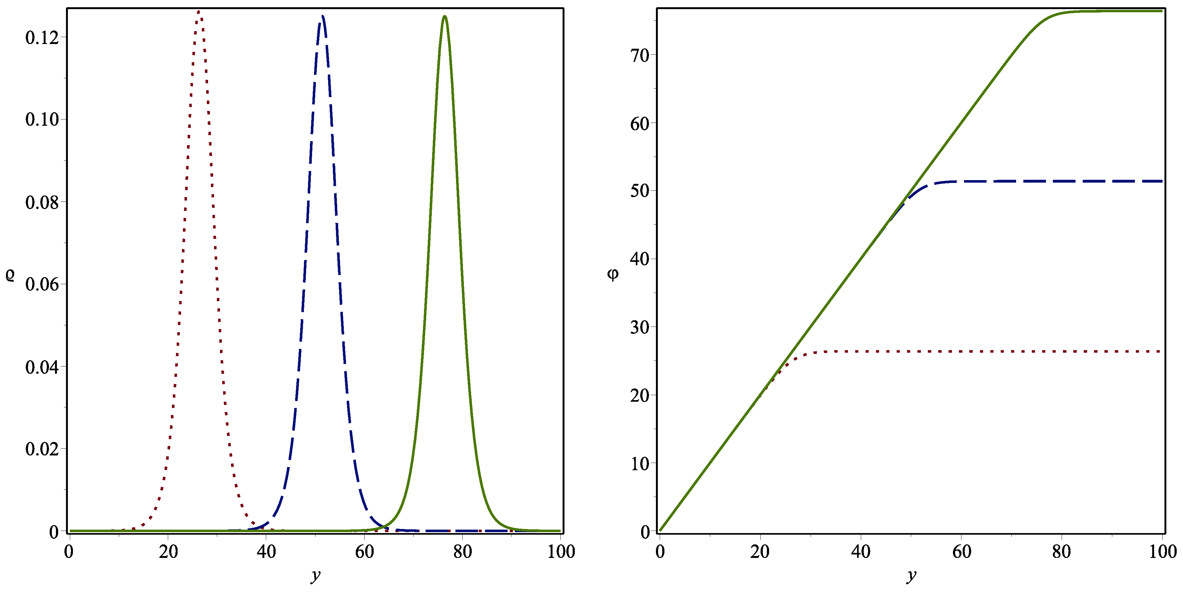
where $h\left(t\right)$ is an arbitrary smooth function. Plots of Solution (18) are presented on Figure 1. It should be noted that the very similar profile of the function ρ which describes density of cells was presented in many papers (see, e.g., [2,17,18,19]). However, in papers [2,17,18] the traveling wave solutions were found, and in [19] the numerical ones. So the exact Solution (18) is new because it is neither traveling wave solution nor numerical. It possesses much more complicated structure. Nevertheless this profile of the function ρ represents the traveling band of cells. This phenomenon was studied by J. Adler in his experiments which were described in [20].

Figure 1. Plots of functions $\varrho (t,y)$ and $\phi (t,y)$ with $q_2^0=1,h\left(t\right)=0$ and $t=50$ (dot line), $t=100$ (dash line), $t=150$ (solid line).

Figure 1. Plots of functions $\varrho (t,y)$ and $\phi (t,y)$ with $q_2^0=1,h\left(t\right)=0$ and $t=50$ (dot line), $t=100$ (dash line), $t=150$ (solid line).

Consider Case 2 in Table 2. The linear combination of operators $a_1{G}_1^{\infty }+a_3{X}_S^{\infty }+D$ produces the following ansatz

$$\begin{array}{l}\mathrm{\rho }(t,x,y)=\frac{1}{t}\psi ({\mathrm{\omega }}_1,{\mathrm{\omega }}_2),\\ S(t,x,y)=\varphi ({\mathrm{\omega }}_1,{\mathrm{\omega }}_2)+\frac{a_{1}x}{2\sqrt{t}}\int \frac{f_1^{\prime }\left(t\right)}{\sqrt{t}}dt+\kappa \left(t\right),\\ {\mathrm{\omega }}_1=\frac{x}{\sqrt{t}}-\frac{a_1}{2}\int \frac{f_1\left(t\right)}{t^{\frac{3}{2}}}dt,\\ {\mathrm{\omega }}_2=\frac{y}{\sqrt{t}}\end{array}$$

(19)

where $\kappa \left(t\right)$ is an arbitrary smooth function.

This ansatz reduces BVP (6) to the elliptic BVP

$$\begin{array}{l}▵\psi -\nabla \left(\psi \nabla \varphi \right)+\frac{{\mathrm{\omega }}_1}{2}{\psi }_{{\mathrm{\omega }}_1}+\frac{{\mathrm{\omega }}_2}{2}{\psi }_{{\mathrm{\omega }}_2}+\psi =0,\\ \psi +▵\varphi =0\end{array}$$

(20)

$$\begin{array}{l}{\mathrm{\omega }}_2=0:{\psi }_{{\mathrm{\omega }}_2}=q_1^0,{\varphi }_{{\mathrm{\omega }}_2}=q_2^0,\\ {\mathrm{\omega }}_2=+\infty :{\psi }_{{\mathrm{\omega }}_2}={\varphi }_{{\mathrm{\omega }}_2}=0\end{array}$$

(21)

It can be easily established that System (20) is invariant w.r.t. the 4-dimensional MAI generated by the operators

$$P_1=\frac{\partial }{\partial {\mathrm{\omega }}_1}+\frac{{\mathrm{\omega }}_1}{2}\frac{\partial }{\partial \varphi },P_2=\frac{\partial }{\partial {\mathrm{\omega }}_2}+\frac{{\mathrm{\omega }}_2}{2}\frac{\partial }{\partial \varphi },P_3=\frac{\partial }{\partial \varphi },P_4={\mathrm{\omega }}_2\frac{\partial }{\partial {\mathrm{\omega }}_1}-{\mathrm{\omega }}_1\frac{\partial }{\partial {\mathrm{\omega }}_2}$$

In quite a similar way as it was done for BVP (6) we have proved that only operators $P_1$ and $P_3$ are the Lie symmetry operators of BVP (20) and (21). The linear combination of these operators $P_1+\lambda P_3=\frac{\partial }{\partial {\mathrm{\omega }}_1}+(\lambda +\frac{{\mathrm{\omega }}_1}{2})\frac{\partial }{\partial \varphi },\lambda \in \mathbb{R}$ produces ansatz:

$$\begin{array}{l}\psi ({\mathrm{\omega }}_1,{\mathrm{\omega }}_2)={\psi }_{*}\left({\mathrm{\omega }}_2\right),\\ \varphi ({\mathrm{\omega }}_1,{\mathrm{\omega }}_2)={\varphi }_{*}\left({\mathrm{\omega }}_2\right)+\frac{{\mathrm{\omega }}_1^2}{4}+\lambda {\mathrm{\omega }}_1\end{array}$$

which reduces the Elliptic BVP (20) and (21) to the problem for the second-order ODEs

$$\begin{array}{l}{\psi }_{*}^{″}-{\left({\psi }_{*}{\varphi }_{*}^{\prime }\right)}^{\prime }+\frac{{\mathrm{\omega }}_2}{2}{\psi }_{*}^{\prime }+\frac{1}{2}{\psi }_{*}=0,\\ {\varphi }_{*}^{″}+{\psi }_{*}+\frac{1}{2}=0,\\ {\mathrm{\omega }}_2=0:\frac{\partial {\psi }_{*}}{\partial {\mathrm{\omega }}_2}=q_1^0,\frac{\partial {\varphi }_{*}}{\partial {\mathrm{\omega }}_2}=q_2^0,\\ {\mathrm{\omega }}_2=+\infty :\frac{\partial {\psi }_{*}}{\partial {\mathrm{\omega }}_2}=\frac{\partial {\varphi }_{*}}{\partial {\mathrm{\omega }}_2}=0\end{array}$$

(22)

Unfortunately we were unable to solve BVP (22) because the governing system of ODEs is non-integrable. Happily we noted that BVP (20) and (21) is invariant w.r.t. the Q-conditional symmetry operator $\frac{\partial }{\partial {\mathrm{\omega }}_1}$ (in the sense of Definition 2 [15]). The ansatz generated by the operator $\frac{\partial }{\partial {\mathrm{\omega }}_1}$ has the form

$$\begin{array}{l}\psi ({\mathrm{\omega }}_1,{\mathrm{\omega }}_2)=\widehat{\psi }\left({\mathrm{\omega }}_2\right),\\ \varphi ({\mathrm{\omega }}_1,{\mathrm{\omega }}_2)=\widehat{\varphi }\left({\mathrm{\omega }}_2\right)\end{array}$$

(23)

In contrast to the previous ansatz, this one reduces BVP (20) and (21) to the simpler system of ODEs

$$\begin{array}{l}\widehat{{\psi }^{″}}-{\left(\widehat{\psi }\widehat{{\psi }^{\prime }}\right)}^{\prime }+\frac{{\mathrm{\omega }}_2}{2}\widehat{{\psi }^{\prime }}+\widehat{\psi }=0,\\ \widehat{\psi }+\widehat{{\varphi }^{″}}=0\end{array}$$

(24)

with boundary conditions

$$\begin{array}{l}{\mathrm{\omega }}_2=0:{\widehat{\psi }}_{{\mathrm{\omega }}_2}=q_1^0,{\widehat{\varphi }}_{{\mathrm{\omega }}_2}=q_2^0,\\ {\mathrm{\omega }}_2=+\infty :{\widehat{\psi }}_{{\mathrm{\omega }}_2}={\widehat{\varphi }}_{{\mathrm{\omega }}_2}=0\end{array}$$

(25)

System (24) can be reduced to the 4-th order ODE

$${\widehat{\varphi }}^{\left(4\right)}+\frac{{\mathrm{\omega }}_2}{2}{\widehat{\varphi }}^{\left(3\right)}-{\left(\widehat{{\varphi }^{″}}\widehat{{\varphi }^{\prime }}\right)}^{\prime }+\widehat{{\varphi }^{″}}=0$$

By integrating this equation twice and then using substitution ${\widehat{\varphi }}^{\prime }\left({\mathrm{\omega }}_2\right)=\mathrm{\mu }\left({\mathrm{\omega }}_2\right)$, one can obtain the first order ODE

$${\mathrm{\mu }}^{\prime }-\frac{1}{2}{\mathrm{\mu }}^2+\frac{{\mathrm{\omega }}_2}{2}\mathrm{\mu }+{\mathrm{\mu }}_1^0{\mathrm{\omega }}_2+{\mathrm{\mu }}_2^0=0$$

(26)

where ${\mathrm{\mu }}_0^1,{\mathrm{\mu }}_0^2\in \mathbb{R}$.

In order to construct the general solution of Equation (26), we apply the substitution (see, e.g., [21])

$$U\left({\mathrm{\omega }}_2\right)=e^{-\frac{1}{2}\int \mathrm{\mu }\left({\mathrm{\omega }}_2\right)d{\mathrm{\omega }}_2}$$

Now the linear ODE

$$U^{″}+\frac{{\mathrm{\omega }}_2}{2}{U}^{\prime }+(\frac{1}{2}{\mathrm{\mu }}_1^0{\mathrm{\omega }}_2+\frac{1}{2}{\mathrm{\mu }}_2^0)U=0$$

(27)

is obtained with the general solution:

$$\begin{array}{l}U\left({\mathrm{\omega }}_2\right)=A{e}^{-{\mathrm{\mu }}_1^0{\mathrm{\omega }}_2}K\left({\left({\mathrm{\mu }}_1^0\right)}^2+\frac{1}{2}{\mathrm{\mu }}_2^0,\frac{1}{2},-\frac{1}{4}{({\mathrm{\omega }}_2-4{\mathrm{\mu }}_1^0)}^2\right)+\\ B({\mathrm{\omega }}_2-4{\mathrm{\mu }}_1^0)e^{-{\mathrm{\mu }}_1^0{\mathrm{\omega }}_2}K\left({\left({\mathrm{\mu }}_1^0\right)}^2+\frac{1}{2}{\mathrm{\mu }}_2^0+\frac{1}{2},\frac{3}{2},-\frac{1}{4}{({\mathrm{\omega }}_2-4{\mathrm{\mu }}_1^0)}^2\right)\end{array}$$

where $A,B\in \mathbb{R}$ and $K(a,b,z)$ is Kummer’s function

$$K(a,b,z)=1+{\displaystyle \sum _{k=1}^{\infty }}\frac{{\left(a\right)}_k}{{\left(b\right)}_k}\frac{z^k}{k!},{\left(a\right)}_k=a(a+1)...(a+k-1),{\left(a\right)}_0=1$$

Because Kummer’s functions lead to a very cumbersome solution of BVP in question, we consider the special case ${\mathrm{\mu }}_1^0={\mathrm{\mu }}_2^0=0$ (let us note that more general case ${\mathrm{\mu }}_2^0=-2{\left({\mathrm{\mu }}_1^0\right)}^2$ leads to the same result because of the Boundary conditions (25). In this case Equation (26) has the general solution

$$\mathrm{\mu }\left({\mathrm{\omega }}_2\right)=\frac{e^{-\frac{{\mathrm{\omega }}_2^2}{4}}}{A-\frac{\sqrt{\pi }}{2}erf\left(\frac{{\mathrm{\omega }}_2}{2}\right)}$$

From the Boundary condition (25) follows $\mathrm{\mu }\left(0\right)=\frac{1}{A}=q_2^0$, hence

$$\mathrm{\mu }\left({\mathrm{\omega }}_2\right)=q_2^0\frac{e^{-\frac{{\mathrm{\omega }}_2^2}{4}}}{1-q_2^0\frac{\sqrt{\pi }}{2}erf\left(\frac{{\mathrm{\omega }}_2}{2}\right)}$$

Now one obtains the general solution of BVP (24) and (25)

$$\begin{array}{l}\widehat{\varphi }\left({\mathrm{\omega }}_2\right)=-2ln(1-\frac{q_2^0\sqrt{\pi }}{2}erf\left(\frac{{\mathrm{\omega }}_2}{2}\right)),\\ \widehat{\psi }\left({\mathrm{\omega }}_2\right)=q_2^0\frac{\frac{{\mathrm{\omega }}_2}{2}{e}^{-\frac{{\mathrm{\omega }}_2^2}{4}}(1-q_2^0\frac{\sqrt{\pi }}{2}erf\left(\frac{{\mathrm{\omega }}_2}{2}\right))-q_2^0{e}^{-\frac{{\mathrm{\omega }}_2^2}{2}}}{{(1-q_2^0\frac{\sqrt{\pi }}{2}erf\left(\frac{{\mathrm{\omega }}_2}{2}\right))}^2}\end{array}$$

(28)

Since ${\psi }^{\prime }\left(0\right)=q_1^0$ one can calculate that $q_1^0=\frac{q_2^0}{2}-2{\left(q_2^0\right)}^3$. Thus, the exact solution of BVP (6) with $q_1\left(t\right)=\frac{\frac{q_2^0}{2}-2{\left(q_2^0\right)}^3}{\sqrt{t^3}}$ and $q_2\left(t\right)=\frac{q_2^0}{\sqrt{t}}$ has the form

$$\begin{array}{l}\mathrm{\rho }(t,x,y)=\frac{q_2^0}{t}·\frac{\frac{y}{2\sqrt{t}}{e}^{-\frac{y^2}{4t}}(1-q_2^0\frac{\sqrt{\pi }}{2}erf\left(\frac{y}{2\sqrt{t}}\right))-q_2^0{e}^{-\frac{y^2}{2t}}}{{(1-q_2^0\frac{\sqrt{\pi }}{2}erf\left(\frac{y}{2\sqrt{t}}\right))}^2}\frac{y}{\sqrt{t}},\\ S(t,x,y)=-2ln(1-\frac{q_2^0\sqrt{\pi }}{2}erf\left(\frac{y}{2\sqrt{t}}\right))+\frac{a_{1}x}{2\sqrt{t}}\int \frac{f_1^{\prime }\left(t\right)}{\sqrt{t}}dt+\kappa \left(t\right)\end{array}$$

(29)

where $\kappa \left(t\right)$ is an arbitrary smooth function. Solution (29) is continuous when $q_2^0<\frac{2}{\sqrt{\pi }}$.

4. Conclusions

In this work we studied a simplified version of (1+2)-dimensional Keller–Segel model. It is well-known that Keller–Segel model is widely used for modeling a wide range of processes in biology and medicine (especially for the tumour growth modeling) therefore one is extensively examined by means of different mathematical techniques.

It was established that MAI of System (4) is the infinite-dimensional Lie algebra. Moreover we have proved that different Neumann BVPs for this system of the form (6) still admit infinite-dimensional Lie algebras depending on the form of fluxes $q_1\left(t\right)$ and $q_2\left(t\right)$. Using the definition from [15], all inequivalent problems of the form (6) were found, which admit different MAIs (see Theorem 2).

In order to construct the exact solutions of some Neumann problems, the Lie symmetry operators were applied. In particular, we have proved that the BVP for the one-dimensional (in space) Keller–Segel system in question can be linearized. As result, the exact solution of the BVP was constructed in explicit form (18). It should be stressed that this solution has a remarkable properties, which allow a biological interpretation.

Finally, the exact solution for the (1+2)-dimensional BVP with the correctly specified boundary conditions was found (see Formula (29)).

References

- Keller, E.F.; Segel, L.A. Initiation of slime mold aggregation viewed as an instability. J. Theor. Biol. 1970, 26, 399–415. [Google Scholar] [CrossRef]
- Keller, E.F.; Segel, L.A. Traveling bands of chemotactic bacteria: A theoretical analysis. J. Theor. Biol. 1971, 30, 235–248. [Google Scholar] [CrossRef]
- Horstmann, D. From 1970 until present: the Keller–Segel model in chemotaxis and its consequences. Jahresber. Deutsch. Math. Verein. 2003, 105, 103–165. [Google Scholar]
- Calvez, V.; Dolak-Strub, Y. Asymptotic Behavior of a Two-Dimensional Keller–Segel Model with and without Density Control. Math. Modeling Biol. Syst. 2007, 2, 323–329. [Google Scholar]
- Nagai, T. Convergence to Self-Similar Solutions for a Parabolic–Elliptic System of Drift-Diffusion Type in R2. Adv. Differ. Equ. 2011, 9–10, 839–866. [Google Scholar]
- Nagai, T. Global Existence and Decay Estimates of Solutions to a Parabolic–Elliptic System of Drift-Diffusion Type in R2. Differ. Integral Equ. 2011, 1–2, 29–68. [Google Scholar]
- Fujie, K.; Yokota, T. Behavior of solutions to parabolic–elliptic Keller–Segel systems with signal-dependent sensitivity. In Mathematical Models of Chemotaxis, Proceeding of the 10th AIMS Conference on Dynamical Systems, Differential Equations and Applications, Madrid, Spain, 7–11 July 2014.
- Granero-Belinchon, R.; Ascasibar, Y. On the Patlak–Keller–Segel model with a nonlocal flux. In Mathematical Models of Chemotaxis, Proceeding of the 10th AIMS Conference on Dynamical Systems, Differential Equations and Applications, Madrid, Spain, 7–11 July 2014.
- Cherniha, R.; Didovych, M. Exact solutions of the simplified Keller–Segel model. Commun. Nonlinear Sci. Numer. Simulat. 2013, 18, 2960–2971. [Google Scholar] [CrossRef]
- Fushchych, W.; Cherniha, R. Galilei-invariant systems of nonlinear systems of evolution equations. J. Phys. A Math. Gen. 1995, 28, 5569–5579. [Google Scholar] [CrossRef]
- Hillen, T.; Painter, K.J. A user’s guide to PDE models for chemotaxis. J. Math. Biol. 2009, 58, 183–217. [Google Scholar] [CrossRef]
- Nagai, T. Blow-up of Radially Symmetric Solutions. Adv. Math. Sci. Appl. 1995, 5, 581–601. [Google Scholar]
- Bluman, G.W. Application of the general similarity solution of the heat equation to boundary value problems Q. Appl. Math. 1974, 31, 403–415. [Google Scholar]
- Bluman, W.; Kumei, S. Symmetries and Differential Equations; Springer: Berlin, Germany, 1989. [Google Scholar]
- Cherniha, R.; King, J. Lie and Conditional Symmetries of a Class of Nonlinear (1+2)-dimensional Boundary Value Problems. Symmetry 2015, 7, 1410–1435. [Google Scholar] [CrossRef]
- Polyanin, A.; Manzhirov, A. Handbook of Integral Equations; CRC Press Company: Boca Raton, FL, USA, 1998. [Google Scholar]
- Novick-Cohen, A.; Segel, L. A Gradually Slowing Traveling Band of Chemotactic Bacteria. J. Math. Biol. 1984, 19, 125–132. [Google Scholar] [CrossRef]
- Feltham, D.L.; Chaplain, M.A.J. Travelling Waves in a Model of Species Migration. Appl. Math. Lett. 2000, 13, 67–73. [Google Scholar] [CrossRef]
- Wang, Q. Boundary Spikes of a Keller–Segel Chemotaxis System with Saturated Logarithmic Sensitivity. Disc. Contin. Dyn. Syst. Ser. B 2015, 20, 1231–1250. [Google Scholar] [CrossRef]
- Adler, J. Chemotaxis in bacteria. Ann. Rev. Biochem. 1975, 44, 341–356. [Google Scholar] [CrossRef]
- Polyanin, A.; Zaitsev, V. Exact Solutions for Ordinary Differential Equations; CRC Press: Boca Raton, FL, USA, 2003. [Google Scholar]
© 2015 by the author; licensee MDPI, Basel, Switzerland. This article is an open access article distributed under the terms and conditions of the Creative Commons Attribution license (http://creativecommons.org/licenses/by/4.0/).
Share and Cite
MDPI and ACS Style
Didovych, M. A (1+2)-Dimensional Simplified Keller–Segel Model: Lie Symmetry and Exact Solutions. Symmetry 2015, 7, 1463-1474. https://doi.org/10.3390/sym7031463
AMA Style
Didovych M. A (1+2)-Dimensional Simplified Keller–Segel Model: Lie Symmetry and Exact Solutions. Symmetry. 2015; 7(3):1463-1474. https://doi.org/10.3390/sym7031463
Chicago/Turabian StyleDidovych, Maksym. 2015. "A (1+2)-Dimensional Simplified Keller–Segel Model: Lie Symmetry and Exact Solutions" Symmetry 7, no. 3: 1463-1474. https://doi.org/10.3390/sym7031463