An Efficient Approach for Sidelobe Level Reduction Based on Recursive Sequential Damping


Department of Computer Engineering, College of Computers and Information Technology, Taif University, P.O. Box 11099, Taif 21944, Saudi Arabia
*
Author to whom correspondence should be addressed.
Symmetry 2021, 13(3), 480; https://doi.org/10.3390/sym13030480
Submission received: 28 February 2021
/
Revised: 10 March 2021
/
Accepted: 12 March 2021
/
Published: 15 March 2021
(This article belongs to the Section Computer)
Abstract
:Recently, antenna array radiation pattern synthesis and adaptation has become an essential requirement for most wireless communication systems. Therefore, this paper proposes a new recursive sidelobe level (SLL) reduction algorithm using a sidelobe sequential damping (SSD) approach based on pattern subtraction, where the sidelobes are sequentially reduced to the optimum required levels with near-symmetrical distribution. The proposed SSD algorithm is demonstrated, and its performance is analyzed, including SLL reduction and convergence behavior, mainlobe scanning, processing speed, and performance under mutual coupling effects for uniform linear and planar arrays. In addition, the SSD performance is compared with both conventional tapering windows and optimization techniques, where the simulation results show that the proposed SSD approach has superior maximum and average SLL performances and lower processing speeds. In addition, the SSD is found to have a constant SLL convergence profile that is independent on the array size, working effectively on any uniform array geometry with interelement spacing less than one wavelength, and deep SLL levels of less than −70 dB can be achieved relative to the mainlobe level, especially for symmetrical arrays.
1. Introduction
1.1. Background and Motivation
Antenna arrays and beamforming systems have become essential parts for most recent wireless communication systems and play important roles in the provision of high capacities and data rates. Signals can be received more efficiently, and the system performance can be enhanced greatly by using beamforming techniques with antenna arrays such as in multiple-input multiple-out (MIMO) mobile systems, radar, sonar, satellite, and many other recent applications, such as wireless sensors and medical networks [1,2,3,4,5,6,7,8]. To improve the system capacity and provide higher data rates for users, it is necessary to utilize millimeter wave frequencies such as in the fifth-generation (5G) mobile systems and networks beyond that, where larger bandwidths are available. However, the millimeter wave frequencies are characterized by high atmospheric propagation losses and require being boosted by efficient antenna array systems [9]. One of the most important capabilities of antenna arrays is the capability to concentrate the radiation pattern in the desired directions and control the level of unwanted radiations such as the sidelobes, which usually collect the unwanted interfering signals. Therefore, providing a high-gain mainlobe while reducing the sidelobe levels (SLLs) is one of the most important requirements for achieving a higher signal-to-interference ratio and spectral efficiency. There are many SLL reduction techniques in the literature, including simple constant tapering windows [10,11,12,13,14,15], optimized tapering windows [16,17,18], and many other efficient optimization techniques [19,20,21,22,23,24,25,26,27,28,29]. These techniques differ in complexity, ranging from simple straightforward feeding as in the tapered beamforming techniques to more sophisticated optimization techniques that optimize the array parameters to achieve the required optimum levels. Tapering window functions can provide very deep sidelobe levels but suffer from the lack of adaptability and may result in very wide beamwidths. Optimized tapering windows, such as Dolph-Chebyshev, Taylor, and Kaiser windows [16,17,18,30], are efficient at reducing SLLs, especially for small-sized arrays. The Dolph-Chebyshev window provides the smallest beamwidth at a certain SLL among other tapered window techniques [30]. On the other hand, swarm optimization techniques are effective for designing antenna arrays of any size [29] without the constraints found in [16,17]. For nonuniform linear antenna arrays, genetic algorithms (GAs) [28] can be used for SLL reduction, while particle swarm optimization (PSO) [20] is used for optimizing circular arrays and concentric ring arrays. Other revolutionary techniques optimize the element currents as well as the element separation distances, such as the firefly algorithm (FA) [22]. Additionally, some techniques focus on suppressing the highest SLL as the main objective, such as the flower pollination algorithm (FPA) [19], cuckoo search algorithm (CS) [23], invasive weed optimization (IWO), biogeography-based optimization (BBO), bat algorithm (BA), whale optimization algorithm (WOA), atom search optimization (ASO) [24,25,26,27], and many other algorithms. Most of these techniques are used for optimizing the radiation patterns of linear and circular antenna arrays, such as FPA, BBO, and IWO, while CS optimizes large planar arrays [29]. For concentric ring arrays, PSO, CS, and FA were examined and proved their efficient SLL reduction. Many comparisons have been conducted between these optimization algorithms, such as in [27,28,29], where the ASO, WOA, FPA, and BA provided much lower SLLs for the same array size compared with the BBO, PSO, IWO, CS, and FA techniques where, for a 16 element uniform linear array (ULA), the lowest SLL of −41 dB relative to the mainlobe level was provided by the ASO algorithm [27], while the highest SLL of −17 dB was obtained using PSO [27,29]. In addition, chicken swarm optimization (CSO) [31] has been developed for simple optimization applications, including SLL reduction. However, it is not suitable for complex optimization problems due to its exploitation ability. The grey wolf optimizer (GWO) [32] is another optimization technique based on a nature-inspired metaheuristic algorithm. In the GWO, the social hierarchy and hunting behavior of gray wolves inspired the optimization process, which is applied in solving many optimization problems, including antenna array pattern synthesis. However, the work done in [32] to improve the SLL level optimized the element locations, which limited the flexibility of application in different communication scenarios. Other optimization techniques, such as the differential search algorithm [33], Taguchi method [34], and backtracking search optimization [35], have been applied to linear array optimization. However, providing a deep SLL requires a larger number of iterations and hence a longer processing time to achieve the optimum solution, which is not suitable for real-time communication scenarios. Additionally, some techniques provide efficient solutions for SLL reduction in specific array geometries while failing in others. For example, tapering window techniques are straightforward for all ULAs, while they can be applied without an optimum solution for planar or concentric ring arrays such as in [13], where the design of the Dolph-Chebyshev window to provide a −80 dB SLL for a linear array provided −40 dB in a uniform concentric ring array. In addition, these fast conventional tapering windows produce constant SLL profiles for a fixed array size and suffer from the lack of adaptation.
1.2. Paper Contribution
To provide a general and array configuration-independent SLL reduction technique with a faster convergence time and adaptive beampattern generation, this paper proposes a recursive, adaptable SLL reduction and control technique by sidelobe sequential damping (SSD), which is performed successively on the local maximum SLL in the radiation pattern. The proposed algorithm starts by finding the maximum SLL, then cancelling it, determining the new resulting weighted vector, proceeding to the resulting next maximum SLL, and so on. The process is continued until the acceptable SLL is reached or the required shape of the radiation pattern is achieved. The proposed technique has adaptation and SLL control capabilities, as in most optimization techniques, but with a faster convergence time, an ability to work on any array configuration with interelement spacing less than one wavelength in distance, and being able to effectively work under mutual coupling. An important feature of the proposed SSD technique is that the number of iterations to find the optimum weights is independent on the array size, and the processing time can be sped up by finding the best angular sampling step sizes. The comparison with various conventional tapering windows shows that the proposed SSD algorithm provides much deeper SLL levels at the same beamwidth and provides a lower average SLL level compared with the Dolph-Chebyshev technique, while the comparison with optimization techniques shows the capability of the SSD algorithm to provide much deeper SLLs with lower average values at a slightly wider beamwidth.
1.3. Paper Organization
Section 2 models the proposed technique, with its performance analyzed in Section 3, while in Section 4, a performance comparison is performed between the proposed SSD technique and various windows and optimization techniques. In Section 5, the impact of mutual coupling on the SSD algorithm is discussed, while Section 6 discusses the application of SSD on two-dimensional planar arrays with the presence of mutual coupling. Section 7 discusses the operational constraints and limitations of the proposed SSD, and finally, Section 8 concludes the paper.
2. Modelling of the Proposed SSD Technique
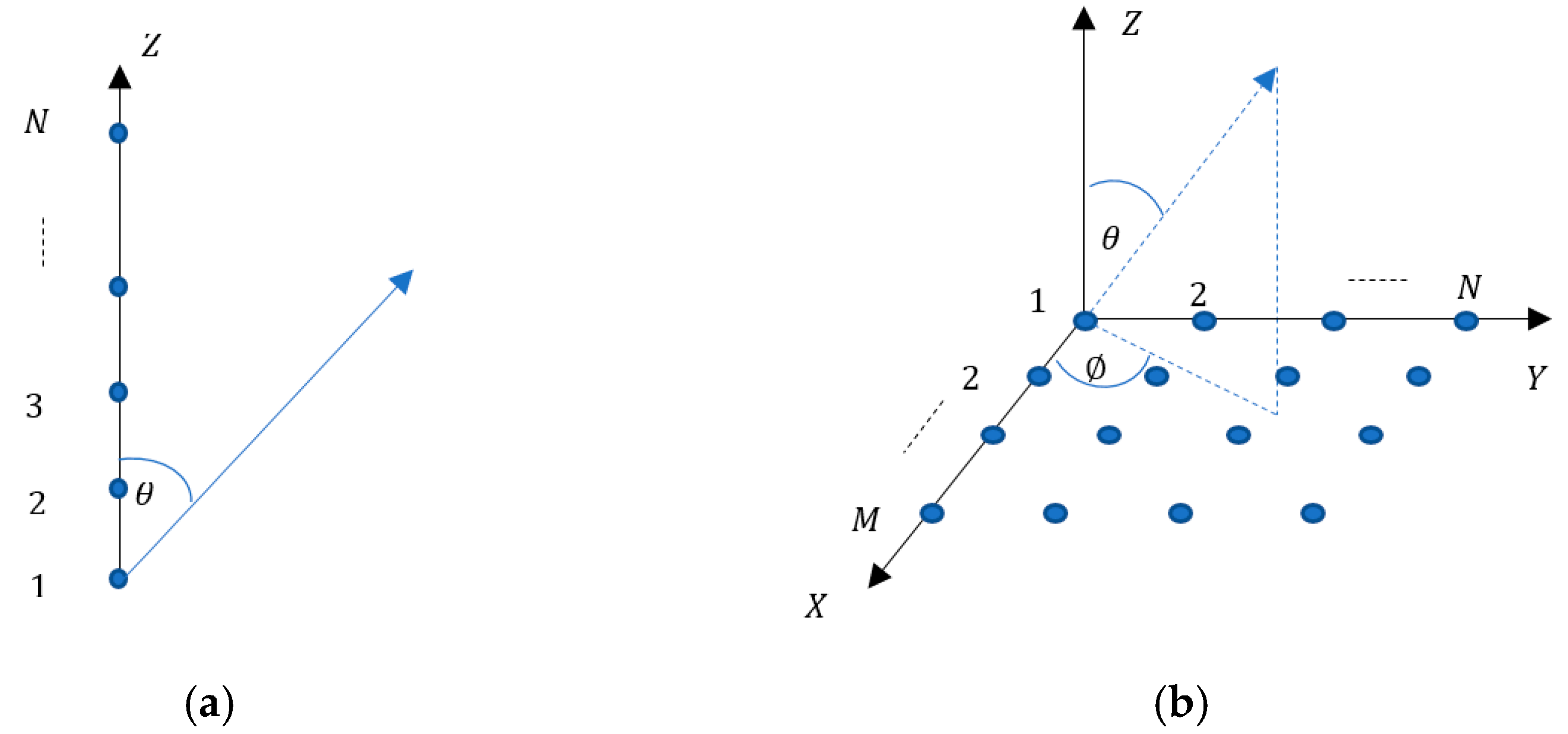
Consider the geometry shown in Figure 1a,b of uniform arrays formed by isotropic antenna elements, with uniform element separation of less than a wavelength in distance and where it is essential to form only one mainlobe in the radiation pattern.
Let us start with the ULA configuration shown in Figure 1a and assume that the antenna elements are weighted by a vector , which is initially set to have unity amplitude coefficients with linear phase shifts to steer the mainlobe toward the desired direction , as in the delay-and-sum beamformer.
In general, the array factor, , can be written as follows:
where is the array steering vector and is the Hermitian operator. For delay-and-sum beamforming, we set , and the array factor is given by
The sidelobe directions, can be obtained by finding the local maxima of , at which the partial derivative with is equal to zero as follows:
where is an infinitesimal angular increment. The set of sidelobe directions is obtained by arranging the corresponding array factor values at in a descending order and excluding the first element in this set, which corresponds to the mainlobe as follows:
where contains the radiation peaks, which include the mainlobe and all sidelobes, and the sidelobe levels vector is therefore given by
and the corresponding sidelobe directions are given by
with the maximum sidelobe gain and direction .
For some uniform array structures, the sidelobe peaks may have an infinite or multiple number of directions with the same level, and in this case, only one peak with any of the directions is selected and inserted into Equation (4) while the others are neglected. The technique in the first iteration will provide perturbation for the array pattern, which eases subsequent sidelobe damping.
To cancel the maximum sidelobe, a secondary mainlobe is formed with the same level and phase as and the same direction as . Then, the array factor of this secondary mainlobe is subtracted from the original array factor as follows:
or
where is the damped sidelobe array factor with only one sidelobe suppressed and is the maximum value of the array factor.
The operation can be repeated to sequentially suppress the sidelobes, where in each cycle, the highest sidelobe is canceled out. After the sidelobe suppression, the overall gain is affected, and the previously suppressed sidelobes may appear diminished, so the actual effect is the damping of the sidelobes rather than nulling them out. If the number of damping cycles is K, then the array factor at the kth damping cycle can be determined according to the following recursive equation:
where is the array gain, corresponding to the uniform feeding case with the highest sidelobe direction at .
The SSD weighting vector, , after damping cycles is given by
The proposed technique can be extended for two-dimensional arrays of a size NM, shown in Figure 1b as follows:
where is the mainlobe direction and K is the number of the damping cycles for SLL reduction in the two dimensions .
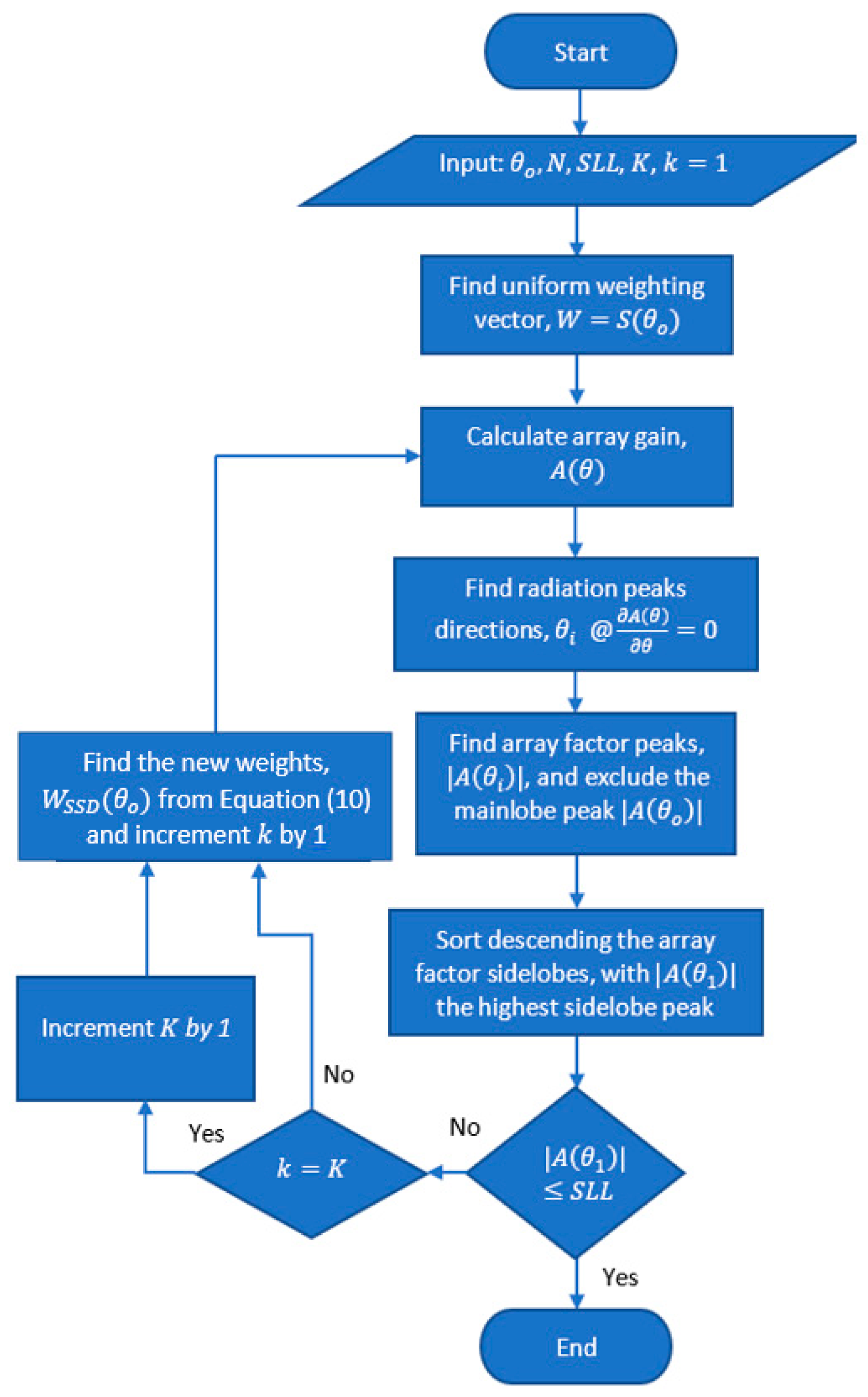
SSD can be performed to achieve a certain SLL by starting with a certain smaller value of and updating it until the required SLL is achieved. The flowchart in Figure 2 demonstrates the iterative SSD, where the initial conditions are first defined and then the sidelobes are sequentially reduced in a one-by-one fashion to achieve the required SLL.
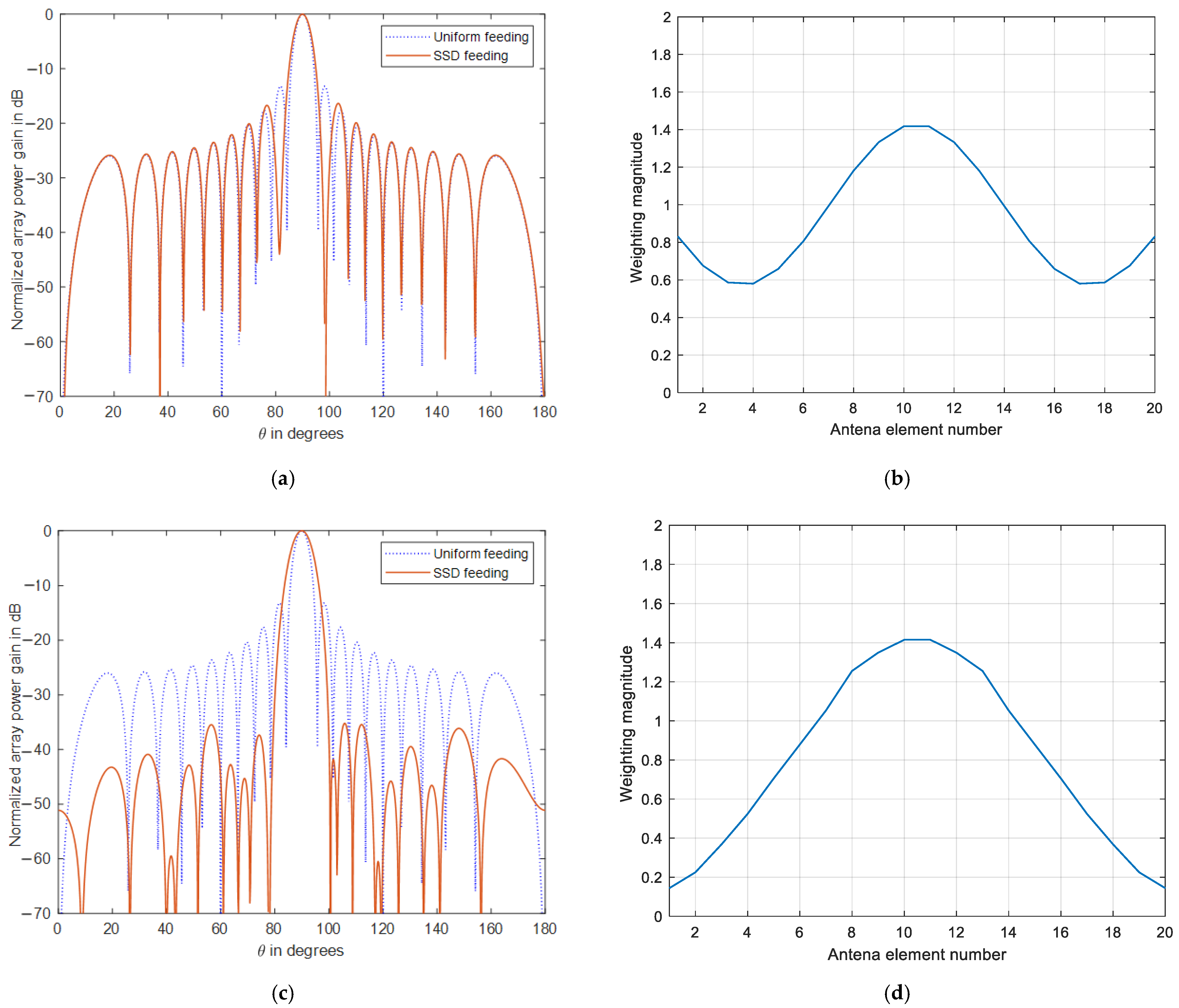
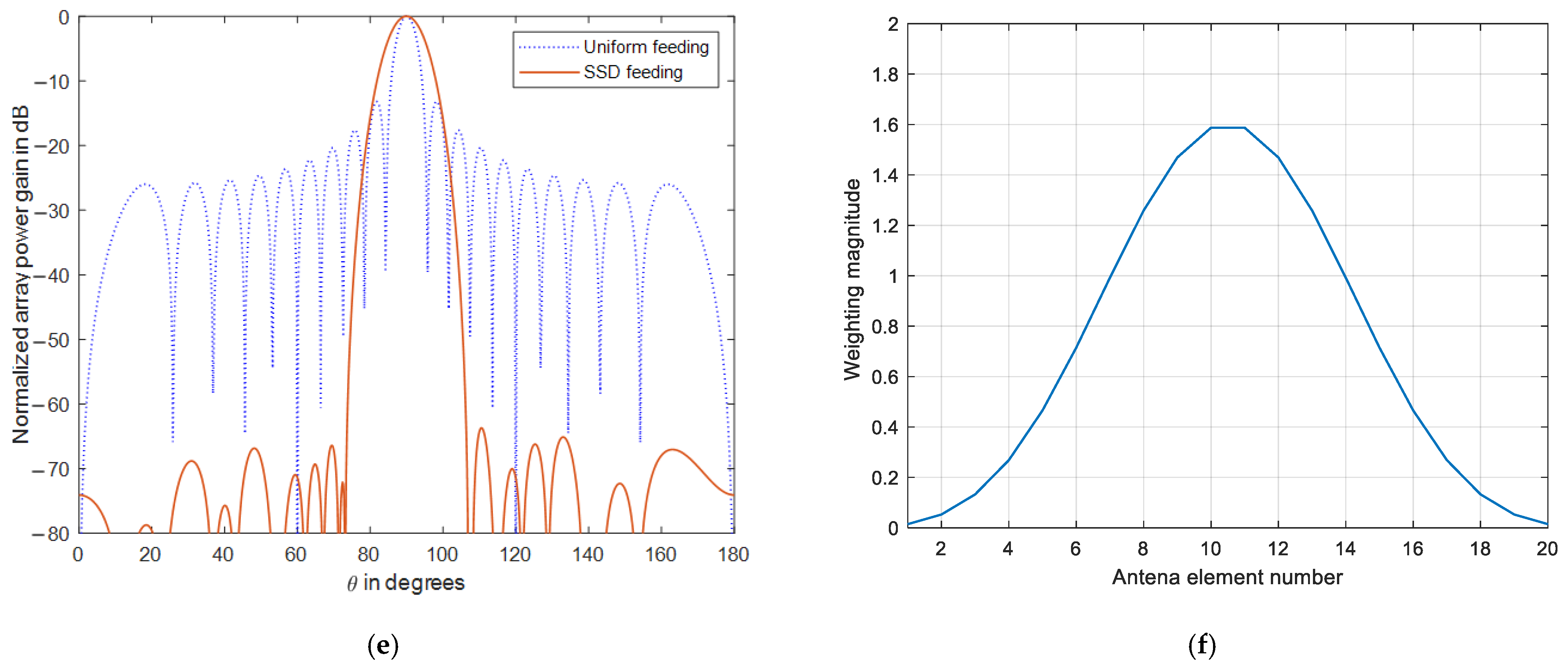
The damping process is examined as shown in Figure 3 for several damping cycles, using the ULA of 20 elements spaced at a distance. In Figure 3a, the two highest sidelobes are damped using two damping cycles, and the resulting array weighting profile is shown in Figure 3b. The operation starts to null the highest sidelobe on the left of the mainlobe, then null the other sidelobe on the right, and the overall result is mainly nulling that on the right while damping the previously canceled out one on the left. Therefore, it is expected after a large number of damping cycles that many sidelobes are damped while the last one is canceled out. In Figure 3c, the number of damping cycles is increased to 50 and the SLL is reduced to −36 dB, and the final weighting profile is shown in Figure 3d. Further increasing the damping cycles will reduce the SLL as shown in Figure 3e, where and the SLL is greatly reduced to dB.
3. SSD Performance Analysis
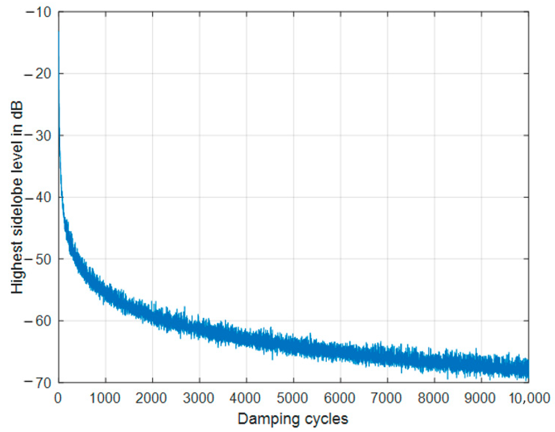
3.1. SSD Damping Behavior
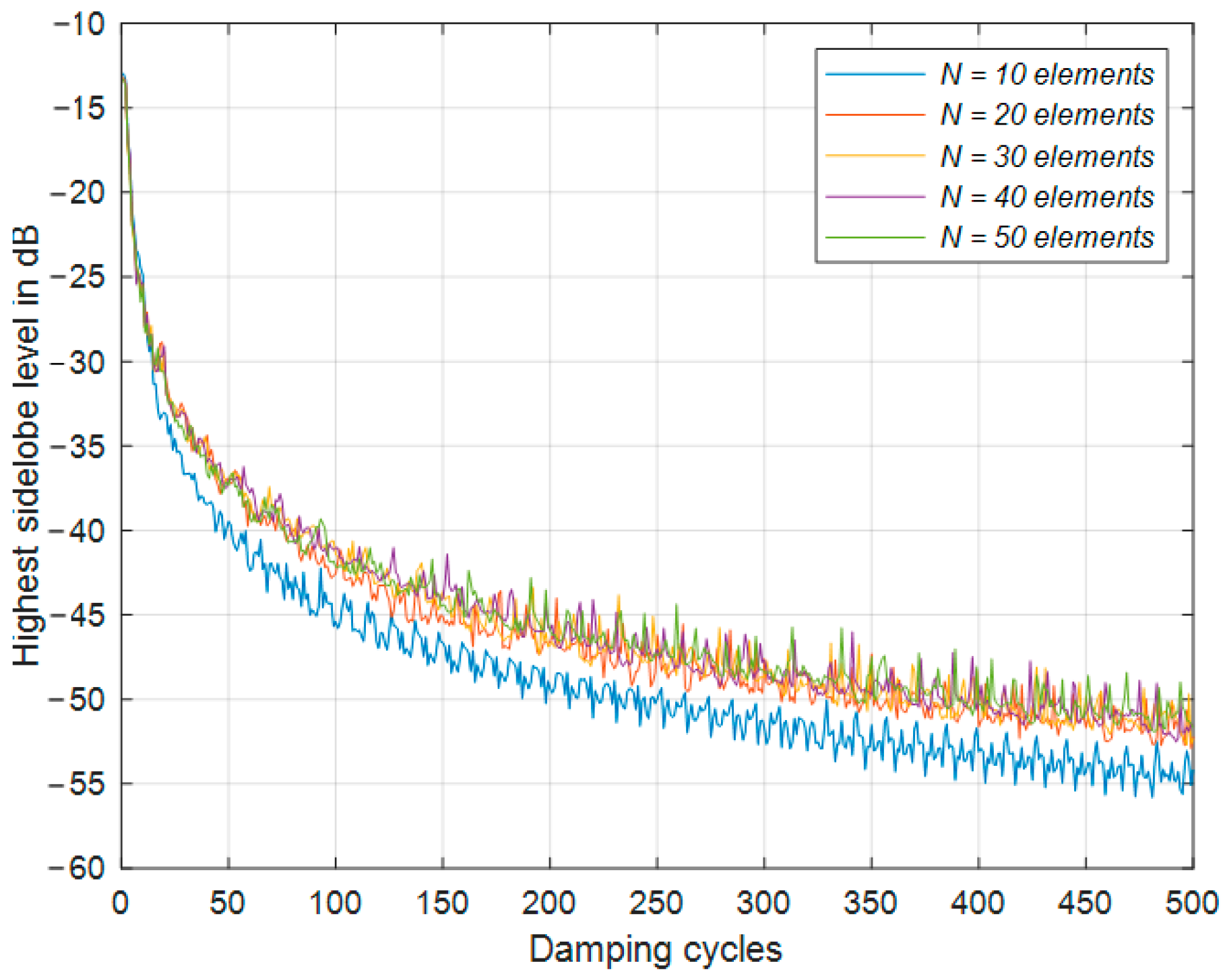
Figure 4 demonstrates the SLL reduction behavior with the number of damping cycles for a 20 element ULA where there was a great and fast reduction in the SLL, especially at the beginning of the SSD damping operation. The SLL dropped to less than dB at values of , while at , it dropped to dB, and further increases in had less of an effect on decreasing the SLL. The damping curve almost had a decaying exponential behavior, where increasing from 1000 to 10,000 reduced the SLL only by approximately 10 dB. This exponential decaying behavior was due to the splitting of the canceled sidelobe peak into two reduced peaks in every damping cycle with some interaction with the neighboring peaks, which may have resulted in slightly increasing their levels. By proceeding with more damping cycles, the sidelobes were decreased in magnitude and became nearly equal in levels, and the possibility of interaction between the subtracted peak from the overall pattern increased with the other nearest peaks, which slowed down the SLL reduction process. However, increases in the damping cycles were always converging to produce lower SLLs, but they required longer processing times due to the interaction between the newly formed sidelobes and the existing ones. On the other hand, the SLL damping profile at different array sizes is shown in Figure 5, where the decaying exponential convergence behavior of the average SLL values had the same rate or profile. For array sizes larger than 10 elements, the SLL reduction by the recursive SSD had the same convergence profile and almost had the same average values. This interesting feature made the proposed SSD technique independent of the array size, where for any array size, we could obtain the same SLL at the same number of damping cycles .
3.2. SSD Behavior at Different Angular Step Sizes
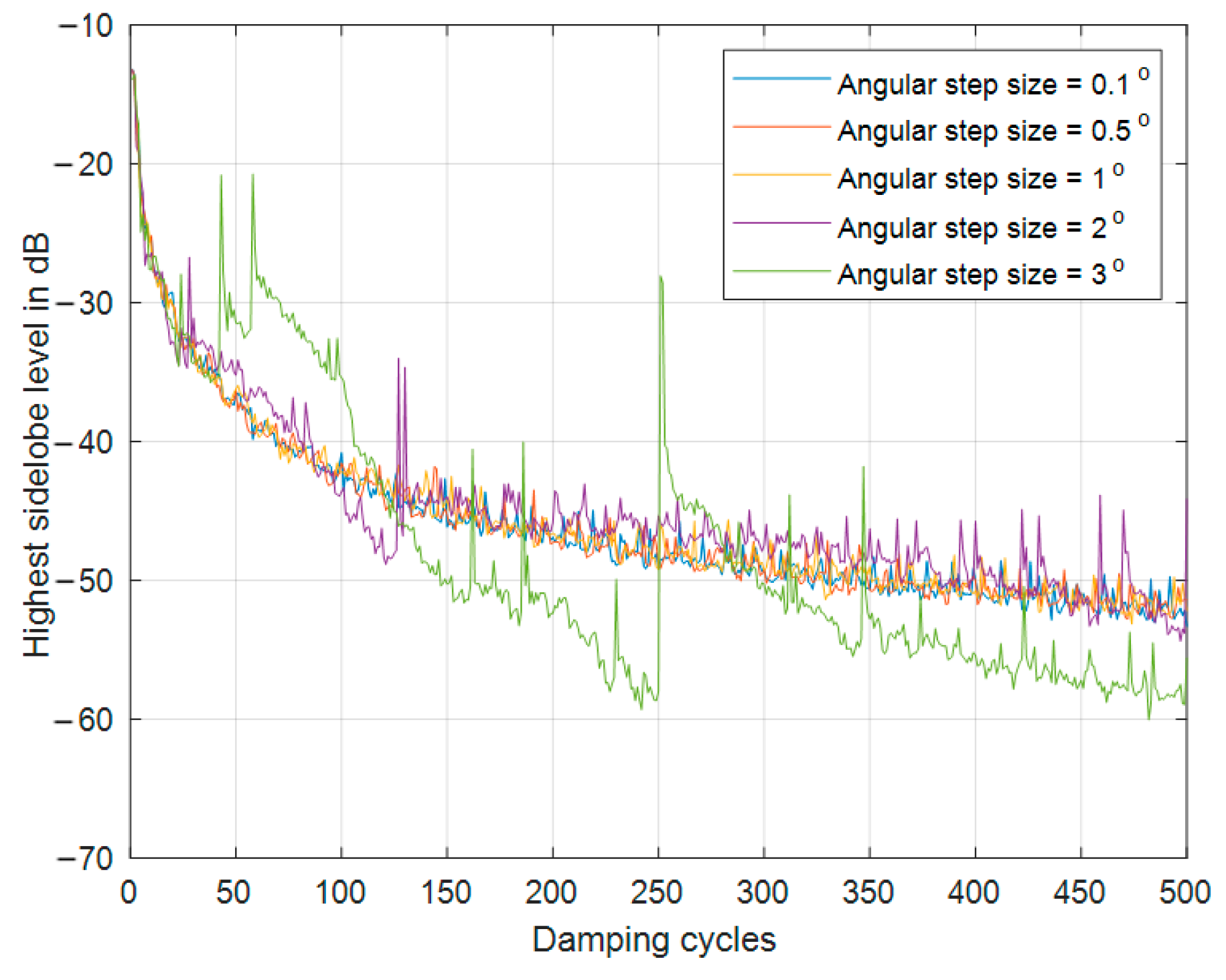
To speed up the recursive SSD algorithm, we should find the directions at which the radiation peaks exist (), and this includes determining the array factor and then finding its peaks and their corresponding , otherwise solving the differential equation in (3), which may be mathematically complicated, especially for large ULA sizes and two-dimensional arrays with a large number of damping cycles. The samples of at the angular steps or increments affected the accuracy of finding and the SLL reduction performance. As shown in Figure 6, for a ULA of 20 elements, an angular resolution or step size greater than 1° resulted in some higher spikes in the damping curve, which resulted from inaccurate directions of the sidelobes, and a retrodictive effect on the SLL reduction process occurred, while for the angular resolution ≤1°, the damping behavior was nominal and converging. However, the overall damping of the SSD converged in a broad sense, and the recursive SSD still worked, but on a rough SLL estimation and in a reduced fashion. In addition, the flowchart presented in Figure 2 provides a solution for the cases where large angular step sizes were used, where the process ended at the accepted SLL regardless of the rough SLL estimation and reduction.
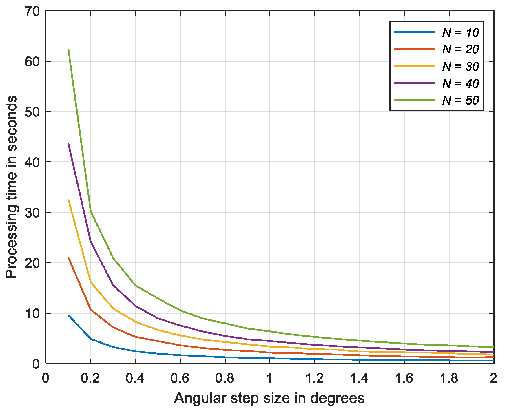
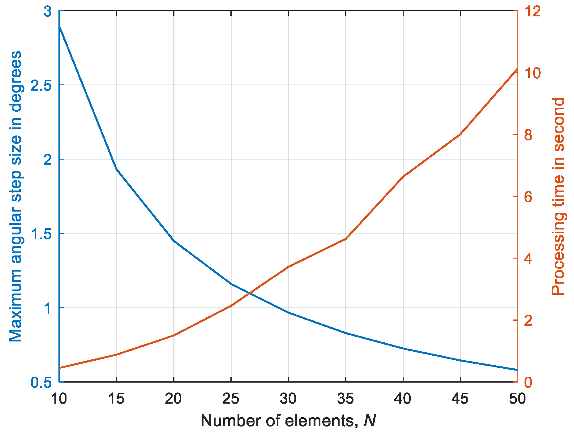
The processing time variation with the sampling angular step sizes for 200 damping cycles at different array sizes is shown in Figure 7, where it varied with exponentially decaying profiles with the angular step size and reduced greatly with the array size. Therefore, choosing the proper value of the angular step size is very important to achieve a lower processing time and smoother convergence to the desired SLL.
A rough estimation for the maximum sampling angular step size could be used as one third of the mainlobe beamwidth, which ensured finding the sidelobe peaks in the provided array factor samples. For the ULA, the maximum sampling angular step size can be considered as follows:
where is the array size. Therefore, the maximum angular step size was adapted with the array size, and this empirical equation was considered as the maximum applicable value for , as shown in Figure 8, which helped in finding fewer samples of and speeding up the processing time. The curves shown in this figure correspond to 200 damping cycles, as previously considered in Figure 7. For two-dimensional arrays, N was considered as the largest number of elements in one of the two directions of the array. Compared to Figure 7, the processing time could be decreased to less than one sixth of its value at = 0.1°, especially for large array sizes.
3.3. Impact of SSD on the Beamwidth
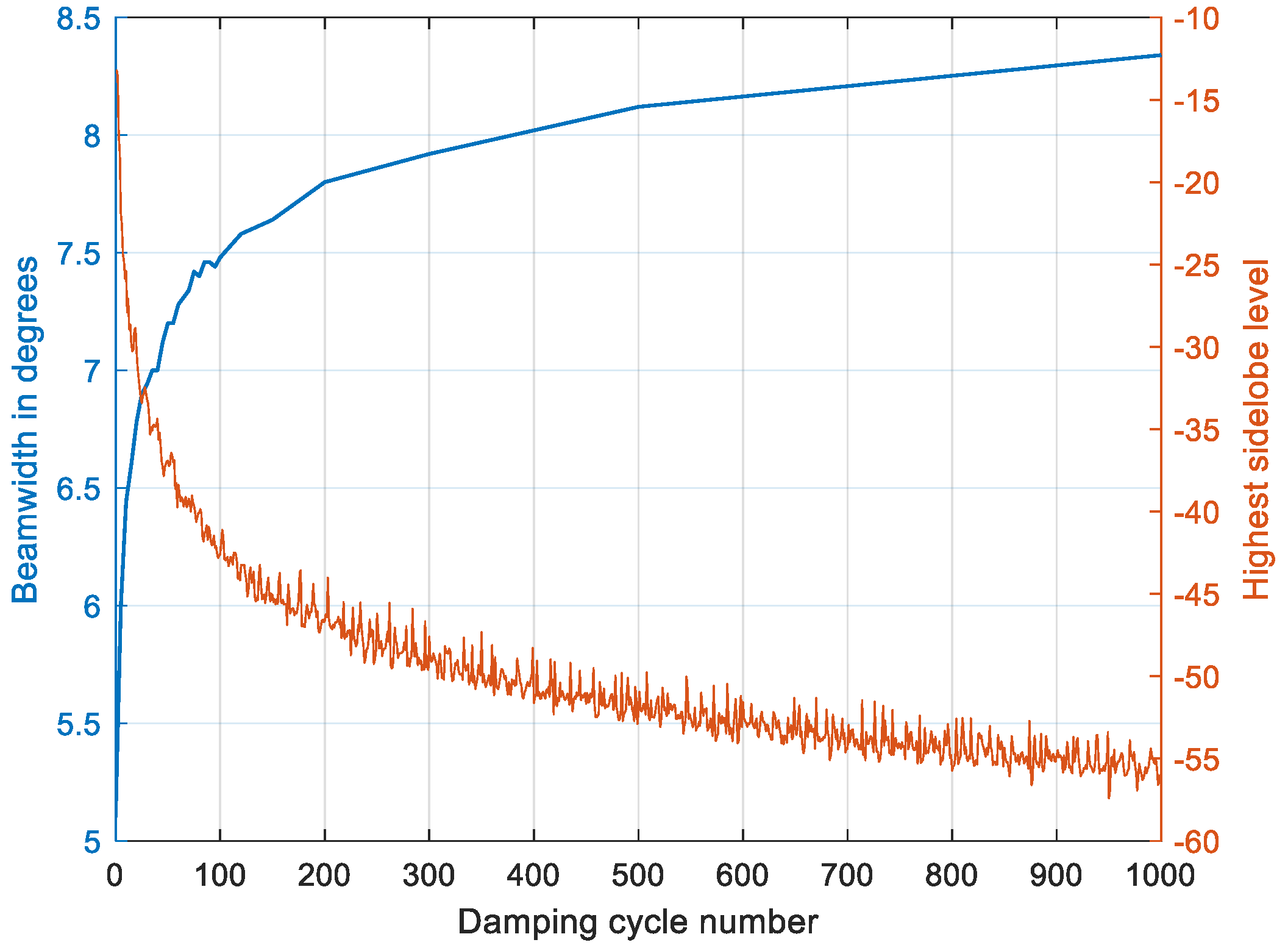
Generally, SLL reduction resulted in an increase in the beamwidth, and so did the proposed SSD technique, as shown in Figure 9 for a 20 element ULA. During the first 100 damping cycles, the beamwidth increased rapidly where the SLL decreased rapidly, while after , the beamwidth increased slightly, where the variation was less than 1° for an increase in from 100 to 1000.
3.4. SSD Performance with Interelement Spacing
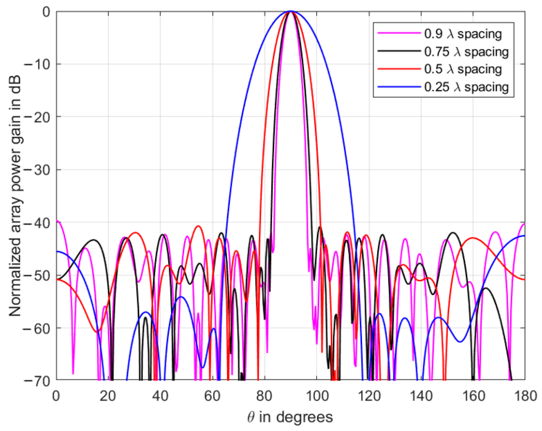
As the proposed SSD algorithm depended on beam space processing, in which the sidelobes were removed sequentially, it would therefore be efficient only for interelement spacing values that were less than one wavelength due to the appearance of secondary major lobes in the visible region. The SSD performance with some typical values of the interelement spacing distance is shown in Figure 10, where the proposed algorithm still worked efficiently at a very low spacing of as well as a very large spacing of . This performance consistency can be interpreted as the SSD also being efficient for wider frequency bands. Furthermore, if the interelement spacing were incorporated in the array synthesis process, the problem of increased beamwidth could be solved while maintaining the required SLL.
3.5. SSD Performance with the Mainlobe Direction
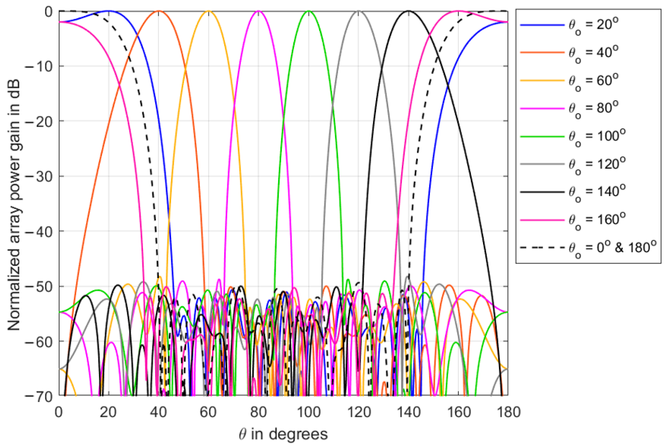
The SSD algorithm was run for obtaining a −50 dB SLL for the 20 element array as shown in Figure 11 at ten various mainlobe directions with 20° steps, and it showed independency with the mainlobe direction. The SLL converged during the recursive SSD process even at = 0° or 180°. This robust performance helped form scanning beams with very low sidelobe levels, which is essential in many practical applications.
4. SSD Performance Comparisons and Discussions
4.1. Comparisons with Conventional Tapering Windows
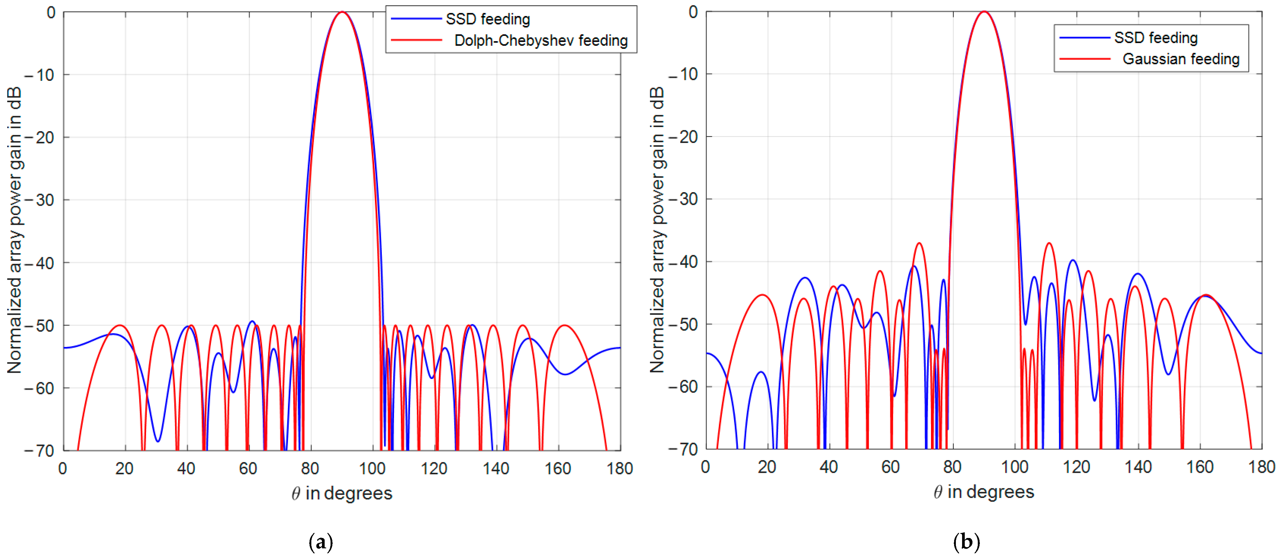
There are many well-known and efficient tapering windows [9] used for SLL reduction, such as triangular (Bartlett), Hamming, Hanning, Dolph-Chebyshev, Kaiser, Blackman, Cosine-square, and Gaussian windows [13]. Among these windows, the Dolph-Chebyshev and Gaussian ones provide the lowest sidelobe levels with a smaller increase in the beamwidth. Therefore, the proposed SSD technique was compared with these two efficient tapering windows as shown in Figure 12a,b. The comparison was based on providing a radiation pattern that had the same beamwidth from the proposed SSD technique and the benchmarking windows. The results shown in Figure 12a,b investigated the SLL performance improvement obtained by the proposed SSD, where the two benchmarking windows provided SLL levels at least 2 dB higher than that achieved by the proposed SSD technique, although the Dolph-Chebyshev window provided the narrowest beamwidth compared with any other window at the same SLL level [9]. The Gaussian window, on the other hand, provided an SLL level that was higher than the proposed SSD technique by 2.83 dB at the same beamwidth, as shown in Figure 12b.
In addition, the property of constant levels of all sidelobes resulting from the Dolph-Chebyshev window was relaxed in the proposed SSD technique, where the average SLL obtained from the Dolph-Chebyshev window was −53.38 dB while that of the SSD technique was −54.4 dB, which was an advantage of 1 dB less for the proposed technique.
Table 1 summarizes the SLL performance comparison between the SSD technique with well-known efficient windows at the same beamwidth. These windows included the triangular, Hamming, Hanning, Blackman, Dolph-Chebyshev, Kaiser, Gaussian, and Kaiser windows. The comparison results in this table show that the SLL obtained from the SSD algorithm at the same beamwidth was lower than any window, where the improvement in the SLL was approximately 12 dB compared with the cosine square window.
4.2. Comparisons with Optimization Techniques
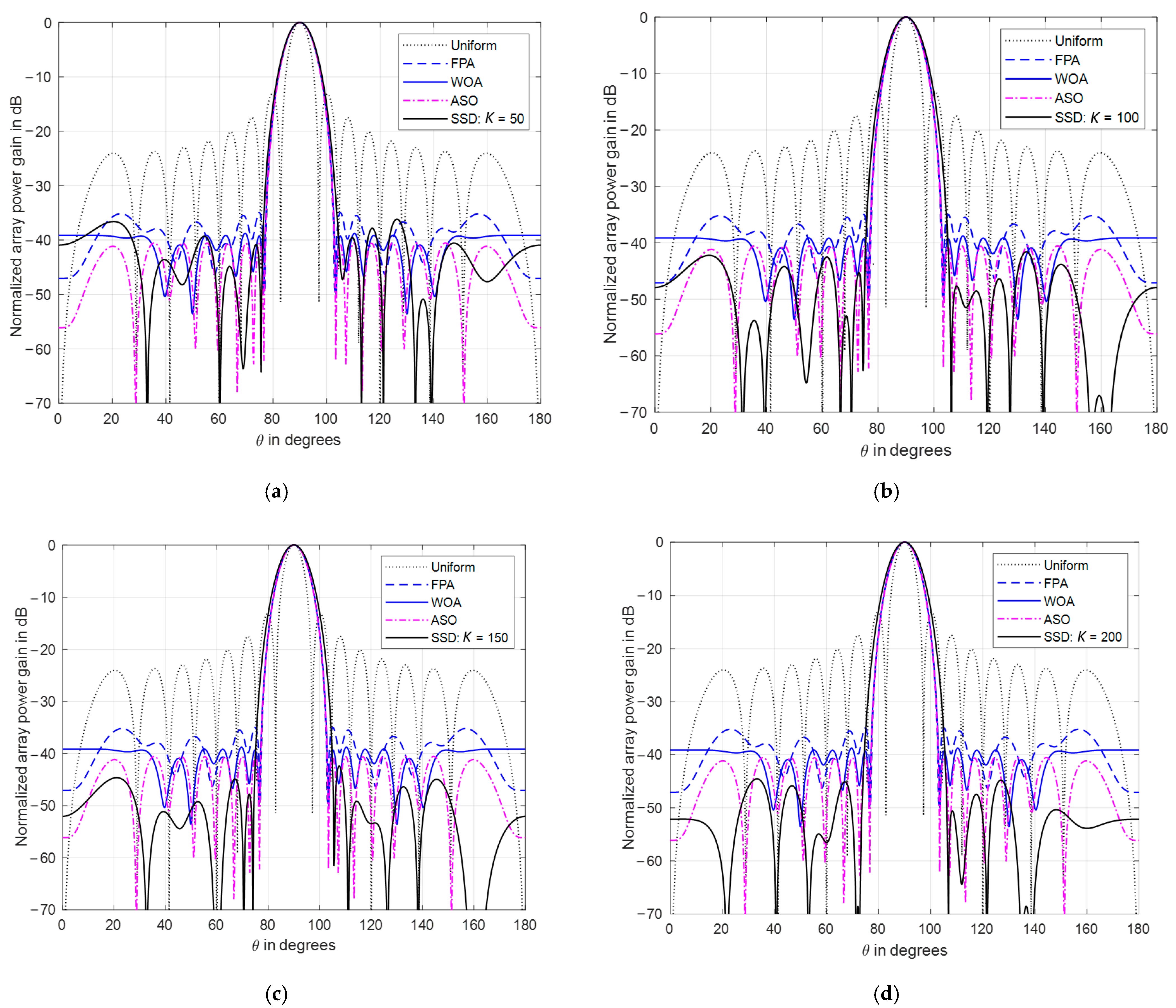
In this section, the proposed SSD SLL reduction technique is compared to some of the most efficient and recent techniques, such as FPA, WOA, ASO, IWO, and CS. These techniques were tested and compared in [27,29] for ULAs of 16 and 32 antenna elements and were examined with the same design parameters presented in these three references for the purpose of comparison with SSD. For the 16 element ULA, the work in [27] showed that the FPA, WOA, and ASO outperformed the PSO and BA algorithms, with the ASO option being the best. Therefore, we compared the proposed SSD algorithm with these three efficient techniques. On the other hand, for the 32 ULA arrays, the work in [29] showed that the IWO and CS methods outperformed FA, BBO and PSO. Therefore we also compared the performance of the proposed SSD algorithm with the ASO, IWO, and CS algorithms. Therefore, comparisons between the proposed SSD algorithm with the PSO, FA, BA, and BBO algorithms were not needed. Starting with the case where the ULA was formed by 16 elements, four values for the number of damping cycles were examined, which were 50, 100, 150, and 200, and the SLL resulting from each was compared with the mentioned optimization techniques as presented in Figure 13a–d.
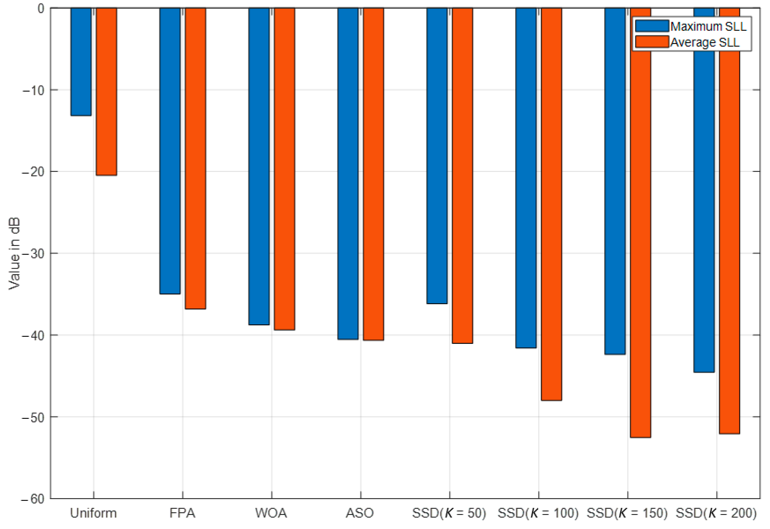
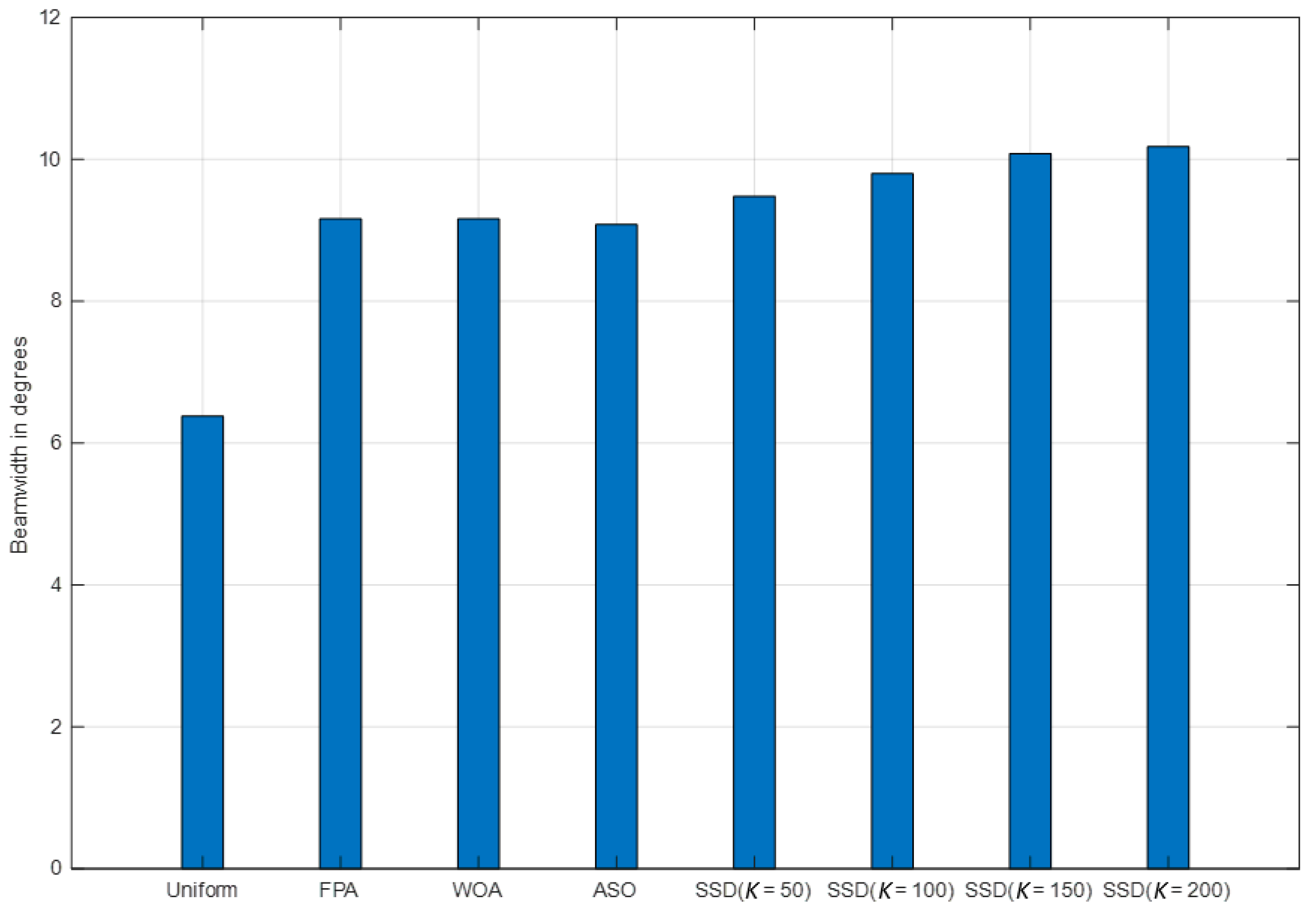
The SSD performance showed lower SLL levels compared with the three efficient techniques, especially at . However, at , the SSD algorithm had better average SLLs than any of the other techniques, as shown in Figure 14. Increasing the value of would improve the SSD performance in terms of both the maximum and average SLLs, where the maximum SLL of −45 dB was lower than the achieved ASO SLL by 4 dB, and the average SLL was −53 dB, which was also lower than that corresponding to ASO by 12 dB at . The processing time consumed by the SSD algorithm was also much smaller than all these techniques, where for the 16 element ULA, the proposed SSD algorithm required only one second at , while the CPU processing time for ASO in [27] was approximately 27 s when using the same platform specification. However, the improved performance of the SLL achieved by SSD compromised slightly wider beams, especially at larger numbers of damping cycles, as shown in Figure 15, where an increase of less than one degree resulted from SSD compared with the ASO at .
On the other hand, the performance improvement in both the maximum and average SLL values obtained from the SSD algorithm came with a price paid in a slightly larger beamwidth (less than 1°) compared with the three optimization techniques, as shown in Figure 15. Therefore, if the slightly increased beamwidth could be tolerated for achieving better SLL performance, then the SSD would be the best choice among the other optimization techniques.
The normalized coefficients of the three optimization techniques, along with the uniform feeding coefficients, are displayed in Figure 16a for a 16 element linear array, while the four cases of the SSD coefficients are displayed in Figure 16b.
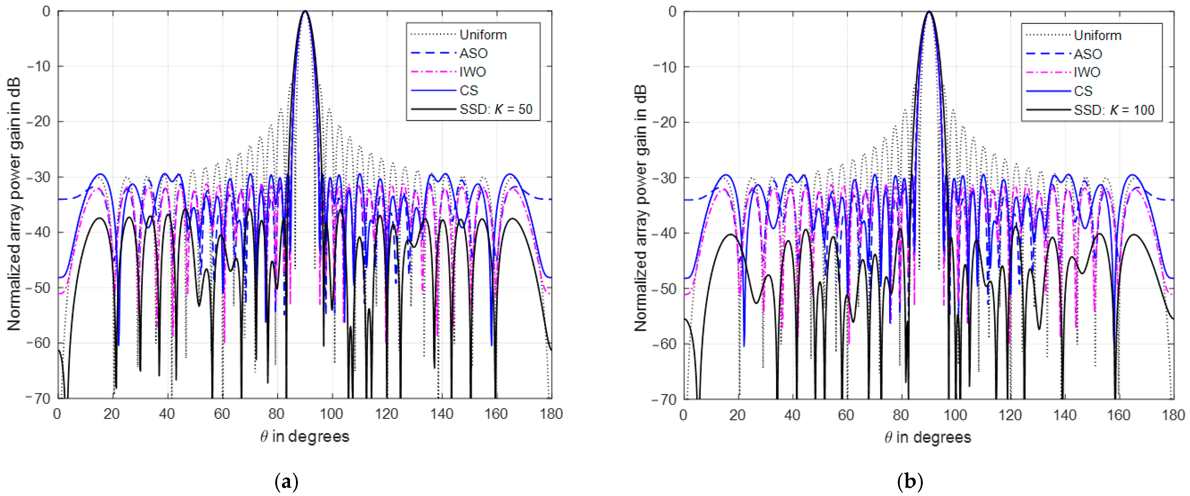
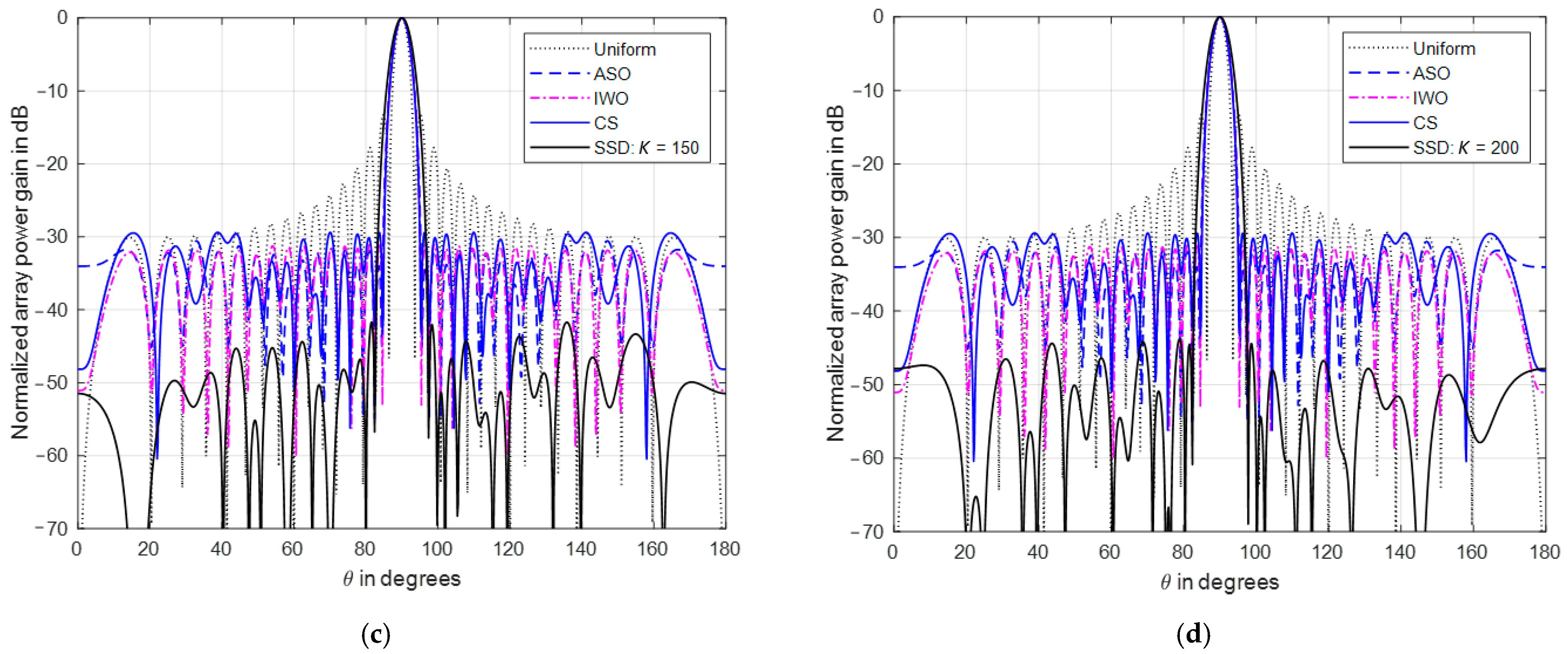
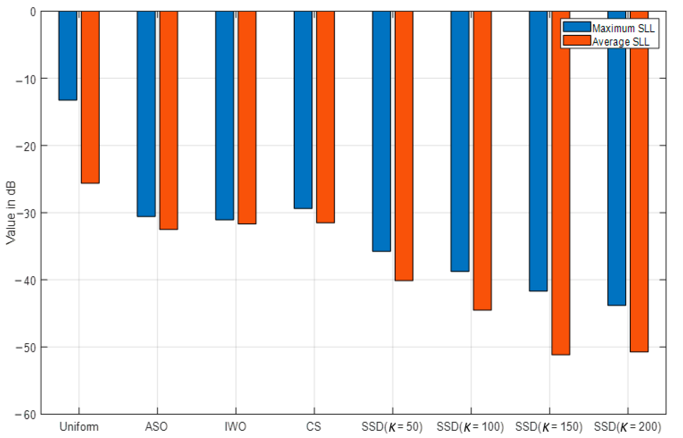
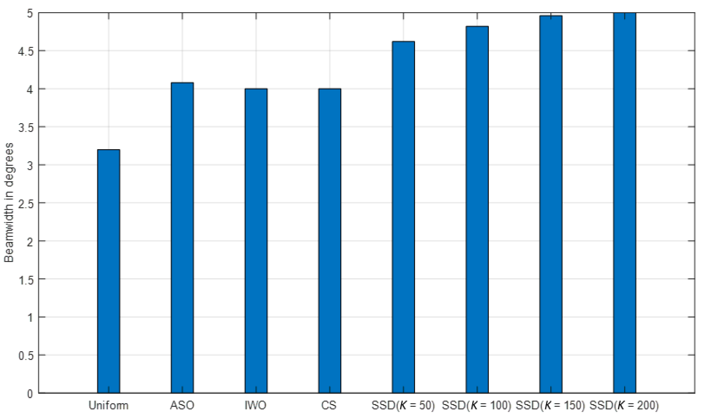
The comparison was also performed for a larger 32 element ULA between the proposed SSD algorithm and the three most efficient techniques in [27,29], which were the ASO, IWO, and CS algorithms, as shown in Figure 17, Figure 18 and Figure 19. As expected, SSD provided a much-improved maximum and average SLL performance—as shown in Figure 18—compared with all of the three techniques, even at lower values of . Moreover, the increase in beamwidth by the SSD technique was less than 0.5° compared with the most efficient ASO technique.
Figure 19 displays the beamwidth values of the different compared techniques at different values of where there was a slight increase, which was less than 1° in the case of the SSD algorithm. Deep SLL levels as low as dB with an average of dB could be achieved, which were much better than the other three algorithms, but at a price of a 0.8° increase in beamwidth.
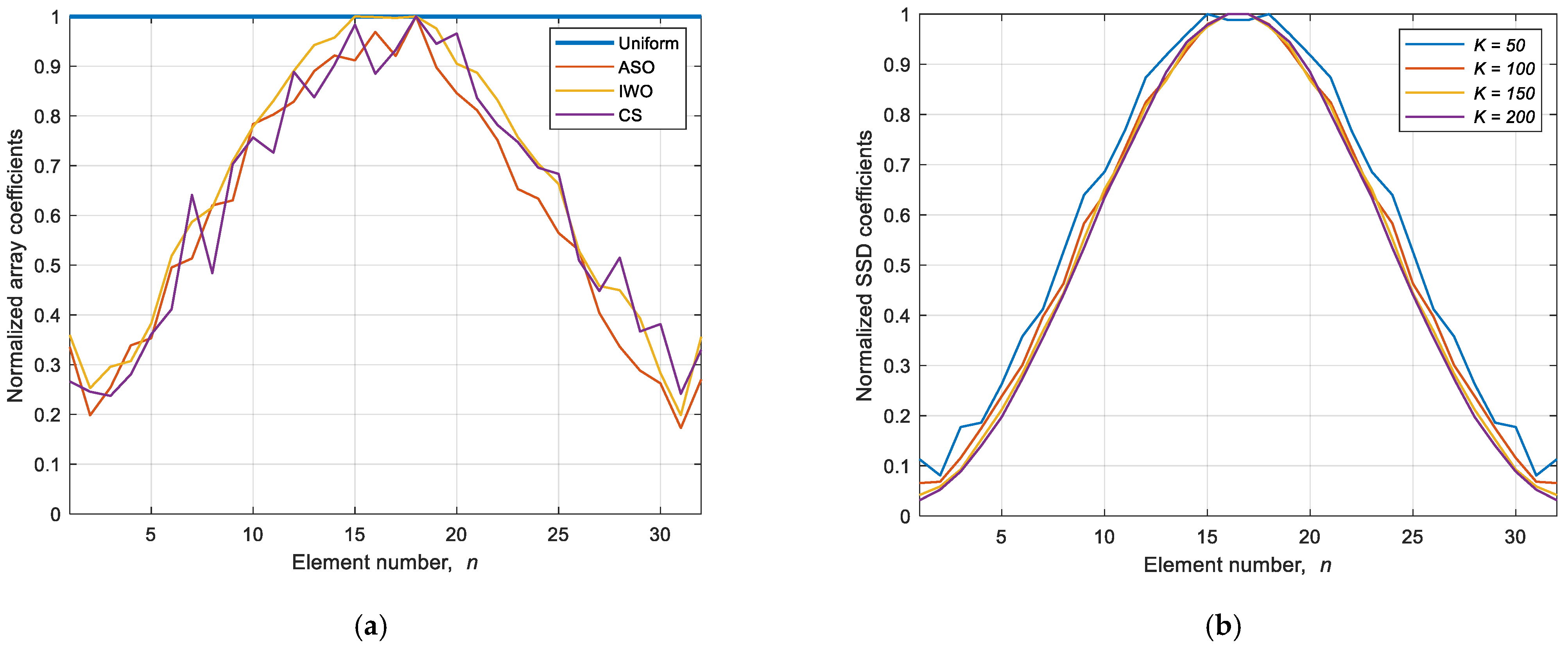
The normalized array coefficients for the 32 element ULA are also displayed Figure 20a for the benchmarking algorithms, while Figure 20b displays the normalized SSD coefficients at different values of , where the curves become steeper at larger values of , increasing the tapering profile and resulting in reducing the SLL to deeper levels.
5. Mutual Coupling Effects on the SSD Performance
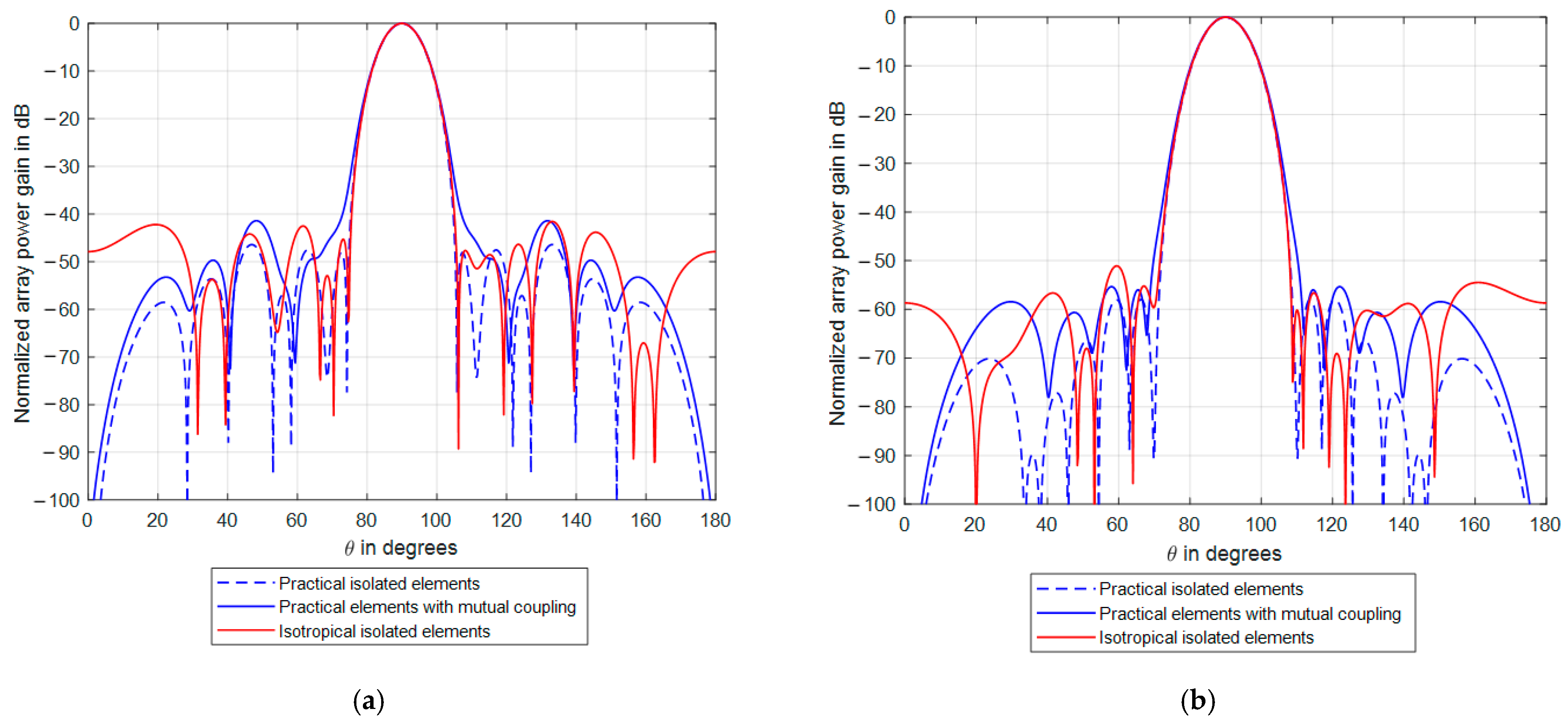
The previous analysis for the SSD technique was performed on isotropic antenna elements, which is now done using practical antenna models along with the inclusion of mutual coupling effects. For a 16 element ULA using half-wave dipoles as antenna elements operating at 5 GHz, Figure 21 displays the resulting normalized radiation patterns at two numbers of damping cycles, namely 100 and 1000. The two sets of curves in this figure include the isotropic isolated antenna elements, practical isolated elements (i.e., without mutual coupling effects), and practical antenna elements with the effect of mutual coupling. For both values of the number of damping cycles, the normalized power patterns displayed very deep SLLs using the SSD algorithm, where the impact of the mutual coupling just appeared to increase in the mainlobe at very low radiation levels below −30 dB. However, the maximum and average SLLs were still very acceptable and sometimes below the isotropic elements case.
6. SSD for Two-Dimensional Planar Arrays
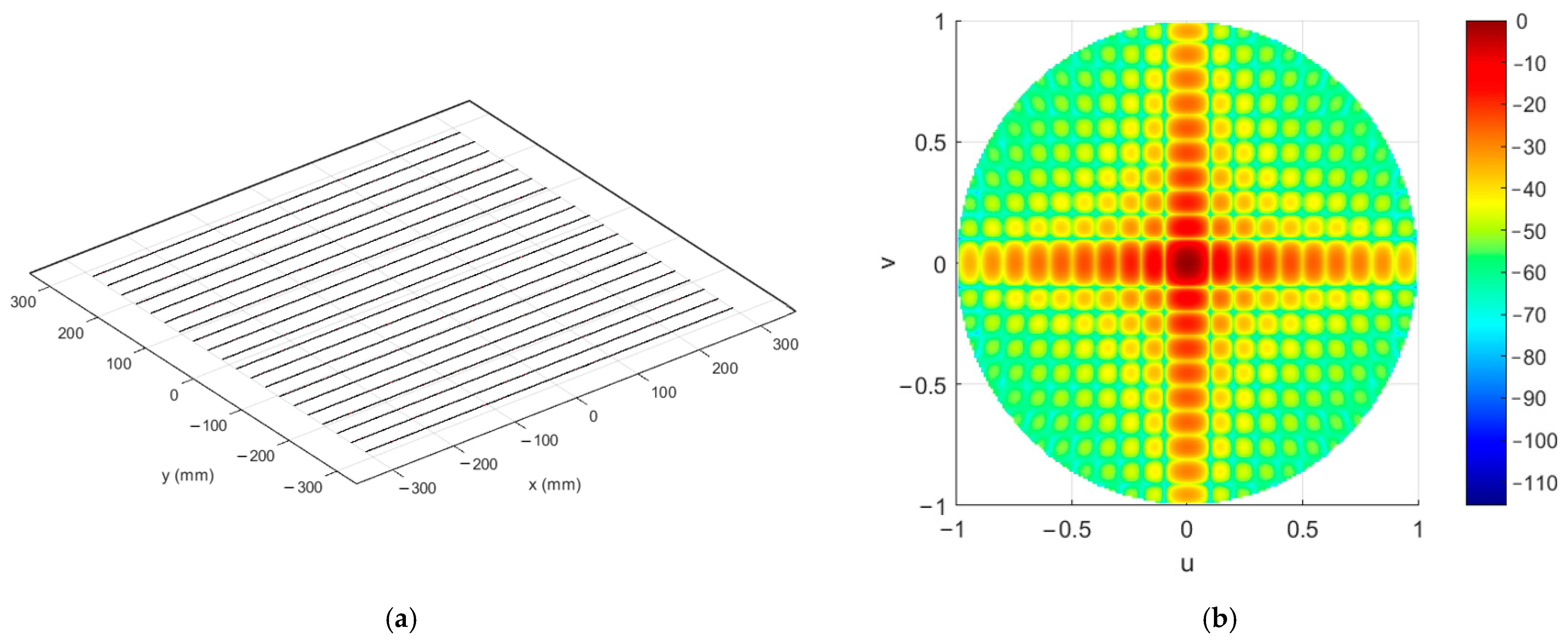
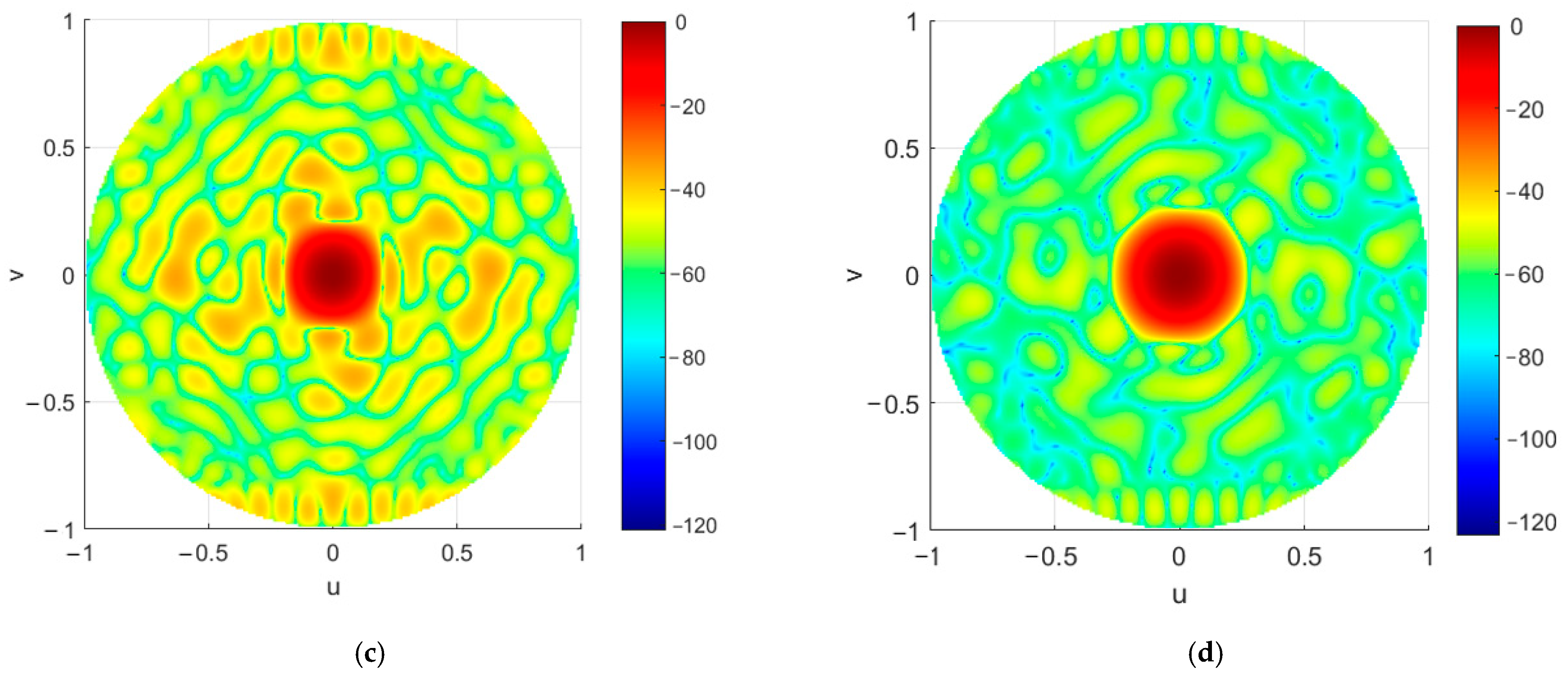
As mentioned in Section 3, the application of the proposed SSD technique was independent of the array configuration and therefore could be applied for any array geometry if there was only one mainlobe in the visible region of the radiation pattern with some relatively lower sidelobes to guarantee SSD convergence. The radiation pattern of a uniformly fed two-dimensional planar array had plenty of sidelobes compared to the ULA, and therefore the SSD damping process required more damping cycles to achieve the required SLL. The process followed the recursive process in Equation (11) and could be examined for a planar array of half-wavelength dipole elements as shown in Figure 22a, operating at 5 GHz with a beam formed in the broadside direction (90°, 0°). The normalized power levels for the uniform feeding case are shown in Figure 22b, and the highest SLL was −13.4 dB relative to the mainlobe level. The improvement in the SLL appeared clearly in Figure 22c with the effect of mutual coupling, where the SLL was reduced to −30 dB at , while it dropped to less than −47 dB at , where 1000 sidelobes had been suppressed from the power pattern.
7. SSD Operational Constraints and Limitations Discussion
In this section, the operational constraints and limitations of the proposed SSD algorithm are explored and discussed. These constraints include the operational interelement spacing and the impact of antenna element failures.
The SSD algorithm was designed mainly for antenna arrays of any configuration that had symmetrical and uniform antenna distributions with interelement spacings that were less than one wavelength. These antenna arrays produce one mainlobe and a set of smaller sidelobes, which allows the SSD to sequentially reduce the sidelobe. If the interelement separation were a distance of more than one wavelength, the SSD could not work as required due to the appearance of secondary major lobes in the radiation pattern, which may have led to the suppression of the required mainlobe. Therefore, in this case, there would be no convergence, and the secondary major lobes would suppress each other in the pattern alternately. The SSD can be modified to select only the sidelobes and exclude the secondary major lobes in Equation (4), so it will work effectively, but without suppression or reduction of the secondary major lobes. However, practically, we almost built arrays with antenna elements separated by a distance that was less than one wavelength—specifically around half the wavelength value—so the SSD could work fine. On the other hand, if the interelement spacing is very small, the SSD still efficiently works, as shown previously in Figure 10, even at a one-quarter wavelength interelement separation, which is practically difficult to implement due to the increase of mutual coupling effects and the physical antenna dimensions.
The second operational constraint for the SSD algorithm is the impact of antenna element failure on the SLL damping performance. If all antenna elements are operating normally, the SSD performs efficiently, but if one or more antenna elements fail or are turned off in the array, then the symmetry structure is perturbed, which affects the SSD SLL reduction performance as the radiation pattern changes. Figure 23 demonstrates the impact of one antenna element’s complete failure at different locations in a 16 element ULA, where it is noticed that the shutdown or malfunctioning antenna elements at the array ends will not affect the SSD damping behavior, and the SSD still works fine. On the other hand, if the failed element is located at the array’s center, then the SSD may fail completely to reduce the SLL, and it is recommended in this case that the number of damping cycles is reduced to the value that gives the best SLL level. The element failure can be expressed in the array steering vector as a zero element, which indicates the absence of that element.
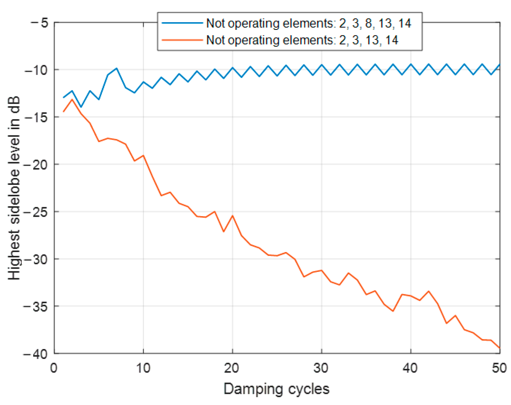
The absence of multiple elements in the array can be handled and tolerated by the SSD algorithm, except in the case where the malfunction element is located at the array’s center. Figure 24 displays this scenario for some of the antenna elements that failed to work in two cases. The first case includes elements 2, 3, 8, 13, and 14, where element 8 represents the central element, which seriously impacts the SSD convergence behavior. On the other hand, the symmetry or near-symmetrical distribution of failed antenna elements, excluding the central antenna, can be handled by the proposed SSD algorithm, which appears to have the robust convergence behavior.
We can conclude from this discussion that the proposed SSD algorithm has robust SLL reduction performance under abnormal operating conditions, which include one or more antenna element failing except for the case where the malfunctioning element is located at the array’s center.
8. Conclusions
Antenna arrays became essential in many recent communication systems to achieve high-quality connectivity performance and higher capacities through proper spatial filtering. Therefore, in this paper, spatial filtering has been achieved by a sequential sidelobe damping algorithm (SSD), where the sidelobes are sequentially damped for sidelobe level (SLL) reduction. The proposed algorithm can be applied for any uniform array geometry, and the SLL can be set to the required level according to the number of the damping cycles. Additionally, the algorithm has been thoroughly analyzed, and the processing time, convergence, and performance with practical scenarios have been investigated, showing independent and very fast convergence times compared with many of the current optimization techniques. In addition, comparisons between the proposed SSD with the well-known windows showed that the SSD achieved lower SLLs at the same beamwidth, while comparisons with many of the recent optimization techniques such as FPA, PSO, WOA, BA, ASO, IWO, FA, CS, and BBO indicated that the proposed SSD can provide lower SLLs at a slightly wider beamwidth, but at a much higher speed of processing and convergence, which is essential in real-time communication scenarios, in addition to the capability of application in any uniform array configuration.
Author Contributions
Conceptualization, Y.A. and F.A.; methodology, Y.A.; software, Y.A.; validation, F.A., and Y.A.; formal analysis, Y.A.; investigation, F.A.; writing—original draft preparation, Y.A.; writing—review and editing, F.A.; visualization, Y.A.; funding acquisition, Y.A. All authors have read and agreed to the published version of the manuscript.
Funding
Taif University Researchers Supporting Project number (TURSP-2020/161), Taif University, Taif, Saudi Arabia.
Acknowledgments
The authors would like to thank Taif University Researchers Supporting Project number (TURSP-2020/161), Taif University, Taif, Saudi Arabia for supporting this work.
Conflicts of Interest
The authors declare no conflict of interest.
References
- Akyildiz, I.F.; Nie, S.; Lin, S.-C.; Chandrasekaran, M. 5G roadmap: 10 key enabling technologies. Comput. Netw. 2016, 106, 17–48. [Google Scholar] [CrossRef]
- Li, J.; Ma, Z.; Mao, L.; Wang, Z.; Wang, Y.; Cai, H.; Chen, X. Broadband Generalized Sidelobe Canceler Beamforming Applied to Ultrasonic Imaging. Appl. Sci. 2020, 10, 1207. [Google Scholar] [CrossRef] [Green Version]
- Wang, Y.; Yang, W.; Chen, J.; Kuang, H.; Liu, W.; Li, C. Azimuth Sidelobes Suppression Using Multi-Azimuth Angle Synthetic Aperture Radar Images. Sensors 2019, 19, 2764. [Google Scholar] [CrossRef] [PubMed] [Green Version]
- Hasan, M.Z.; Al-Rizzo, H. Beamforming Optimization in Internet of Things Applications Using Robust Swarm Algorithm in Conjunction with Connectable and Collaborative Sensors. Sensors 2020, 20, 2048. [Google Scholar] [CrossRef] [Green Version]
- Nguyen, A.H.; Cho, J.-H.; Bae, H.-J.; Sung, H.-K. Side-lobe Level Reduction of an Optical Phased Array Using Amplitude and Phase Modulation of Array Elements Based on Optically Injection-Locked Semiconductor Lasers. Photonics 2020, 7, 20. [Google Scholar] [CrossRef] [Green Version]
- Issa, K.; Fathallah, H.; Ashraf, M.A.; Vettikalladi, H.; Alshebeili, S. Broadband High-Gain Antenna for Millimetre-Wave 60-GHz Band. Electronics 2019, 8, 1246. [Google Scholar] [CrossRef] [Green Version]
- Albagory, Y. An efficient WBAN aggregator switched-beam technique for isolated and quarantined patients. AEU-Int. J. Electron. Commun. 2020, 123, 153322. [Google Scholar] [CrossRef]
- Albagory, Y. Direction-independent and self-reconfigurable spherical-cap antenna array beamforming technique for massive 3D MIMO systems. Wirel. Netw. 2020, 26, 6111–6123. [Google Scholar] [CrossRef]
- Prabhu, K.M.M. Window Functions and Their Applications in Signal Processing; Taylor & Francis: Abingdon, UK, 2014. [Google Scholar]
- Juárez, E.; Panduro, M.A.; Reyna, A.; Covarrubias, D.H.; Mendez, A.; Murillo, E. Design of Concentric Ring Antenna Arrays Based on Subarrays to Simplify the Feeding System. Symmetry 2020, 12, 970. [Google Scholar] [CrossRef]
- Nofal, M.; Aljahdali, S.; Albagory, Y. Tapered beamforming for concentric ring arrays. AEU-Int. J. Electron. Commun. 2013, 67, 58–63. [Google Scholar] [CrossRef]
- Dessouky, M.; Sharshar, H.; Albagory, Y. Optimum normalized-Gaussian tapering window for side lobe reduction in uni-form concentric circular arrays. Prog. Electromagn. Res. 2007, 69, 35–46. [Google Scholar] [CrossRef] [Green Version]
- Dessouky, M.; Sharshar, H.; Albagory, Y. An Approach for Dolph-Chebyshev Uniform Concentric Circular Arrays. J. Electromagn. Waves Appl. 2007, 21, 781–794. [Google Scholar] [CrossRef]
- Dessouky, M.I.; Sharshar, H.A.; Albagory, Y.A. Efficient sidelobe reduction technique for small-sized concentric circular arrays. Prog. Electromagn. Res. 2006, 65, 187–200. [Google Scholar] [CrossRef] [Green Version]
- Nofal, M.; Aljahdali, S.; Albagory, Y. Simplified Sidelobe Reduction Techniques for Concentric Ring Arrays. Wirel. Pers. Commun. 2013, 71, 2981–2991. [Google Scholar] [CrossRef]
- Lau, B.; Leung, Y. A Dolph-Chebyshev approach to the synthesis of array patterns for uniform circular arrays. In Proceedings of the 2000 IEEE International Symposium on Circuits and Systems, Emerging Technologies for the 21st Century, Proceedings (IEEE Cat No. 00CH36353), Geneva, Switzerland, 28–31 May 2000; Volume 1, pp. 124–127. [Google Scholar]
- Sarker, M.A.; Hossain, M.S.; Masud, M.S. Robust beamforming synthesis technique for low side lobe level using taylor excited antenna array. In Proceedings of the 2016 2nd International Conference on Electrical, Computer & Telecommunication Engineering (ICECTE), Rajshahi, Bangladesh, 8–10 December 2016; pp. 1–4. [Google Scholar]
- Aljahdali, S.; Nofal, M.; Albagory, Y. A modified array processing technique based on Kaiser window for concentric circular arrays. In Proceedings of the 2012 International Conference on Multimedia Computing and Systems, ICMCS 2012, Tangiers, Morocco, 10–12 May 2012. [Google Scholar]
- Singh, U.; Salgotra, R. Synthesis of linear antenna array using flower pollination algorithm. Neural Comput. Appl. 2018, 29, 435–445. [Google Scholar] [CrossRef]
- Chakravarthy, V.; Rao, P.M. Circular array antenna optimization with scanned and unscanned beams using novel particle swarm optimization. Indian J. Appl. Res. 2015, 5, 790–793. [Google Scholar]
- Mehrabian, A.; Lucas, C. A novel numerical optimization algorithm inspired from weed colonization. Ecol. Inform. 2006, 1, 355–366. [Google Scholar] [CrossRef]
- Sharaqa, A.; Dib, N. Circular antenna array synthesis using firefly algorithm. Int. J. RF Microw. Comput. Aided Eng. 2014, 24, 139–146. [Google Scholar] [CrossRef]
- Sun, G.; Liu, Y.; Chen, Z.; Zhang, Y.; Wang, A.; Liang, S. Thinning of concentric circular antenna arrays using improved discrete cuckoo search algorithm. In Proceedings of the 2017 IEEE Wireless Communications and Networking Conference (WCNC), San Francisco, CA, USA, 19–22 March 2017; pp. 1–6. [Google Scholar]
- Li, H.; Liu, Y.; Sun, G.; Wang, A.; Liang, S. Beam pattern synthesis based on improved biogeography-based optimization for reducing sidelobe level. Comput. Electr. Eng. 2017, 60, 161–174. [Google Scholar] [CrossRef]
- Van Luyen, T.; Giang, T.V.B. Interference Suppression of ULA Antennas by Phase-Only Control Using Bat Algorithm. IEEE Antennas Wirel. Propag. Lett. 2017, 16, 3038–3042. [Google Scholar] [CrossRef]
- Mirjalili, S.; Lewis, A. The Whale Optimization Algorithm. Adv. Eng. Softw. 2016, 95, 51–67. [Google Scholar] [CrossRef]
- Almagboul, M.A.; Shu, F.; Qian, Y.; Zhou, X.; Wang, J.; Hu, J. Atom search optimization algorithm based hybrid antenna array receive beamforming to control sidelobe level and steering the null. AEU-Int. J. Electron. Commun. 2019, 111, 152854. [Google Scholar] [CrossRef]
- Liang, S.; Fang, Z.; Sun, G.; Liu, Y.; Qu, G.; Zhang, Y. Sidelobe Reductions of Antenna Arrays via an Improved Chicken Swarm Optimization Approach. IEEE Access 2020, 8, 37664–37683. [Google Scholar] [CrossRef]
- Sun, G.; Liu, Y.; Li, H.; Liang, S.; Wang, A.; Li, B. An Antenna Array Sidelobe Level Reduction Approach through Invasive Weed Optimization. Int. J. Antennas Propag. 2018, 2018, 4867851. [Google Scholar] [CrossRef] [Green Version]
- Balanis, C.A. Antenna Theory: Analysis and Design, 4th ed.; Wiley: Hoboken, NJ, USA, 2016; ISBN 978-1-118-64206-1. [Google Scholar]
- Meng, X.; Liu, Y.; Gao, X.; Zhang, H. A New Bio-inspired Algorithm: Chicken Swarm Optimization. In Advances in Swarm Intelligence; Tan, Y., Shi, Y., Coello, C.A.C., Eds.; ICSI: Lecture Notes in Computer Science; Springer: Cham, Switzerland, 2014; Volume 8794. [Google Scholar] [CrossRef]
- Saxena, P.; Kothari, A. Optimal Pattern Synthesis of Linear Antenna Array Using Grey Wolf Optimization Algorithm. Int. J. Antennas Propag. 2016, 2016, 1205970. [Google Scholar] [CrossRef] [Green Version]
- Guney, K.; Durmus, A.; Basbug, S. Antenna Array Synthesis and Failure Correction Using Differential Search Algorithm. Int. J. Antennas Propag. 2014, 2014, 276754. [Google Scholar] [CrossRef] [Green Version]
- Weng, W.-C.; Yang, F.; Elsherbeni, A.Z. Linear antenna array synthesis using Taguchi’s method: A novel optimization technique in electromagnetics. IEEE Trans. Antennas Propag. 2007, 55, 723–730. [Google Scholar] [CrossRef]
- Guney, K.; Durmus, A. Pattern Nulling of Linear Antenna Arrays Using Backtracking Search Optimization Algorithm. Int. J. Antennas Propag. 2015, 2015, 713080. [Google Scholar] [CrossRef] [Green Version]
Figure 1.
Uniform array configurations for (a) a one-dimensional array and (b) a two-dimensional array.
Figure 1.
Uniform array configurations for (a) a one-dimensional array and (b) a two-dimensional array.

Figure 2.
Flowchart representation for the recursive sidelobe sequential damping (SSD) sidelobe level (SLL) reduction algorithm.
Figure 2.
Flowchart representation for the recursive sidelobe sequential damping (SSD) sidelobe level (SLL) reduction algorithm.

Figure 3.
SLL reduction by SSD at different damping cycles. (a) with (b) the weighting profile at , (c) with (d) the weighting profile at , and (e) with (f) the weighting profile at .
Figure 3.
SLL reduction by SSD at different damping cycles. (a) with (b) the weighting profile at , (c) with (d) the weighting profile at , and (e) with (f) the weighting profile at .


Figure 4.
Recursive SSD damping performance.

Figure 5.
Variation of SSD damping with the number of damping cycles at different array sizes.

Figure 6.
SSD damping behavior at variable angular step sizes.

Figure 7.
SSD processing time variation with angular step sizes at variable array sizes.

Figure 8.
Maximum angular step size with the number of elements in the array.

Figure 9.
Beamwidth variation with the number of damping cycles and highest SLL.

Figure 10.
Performance of SSD at different interelement spacings.

Figure 11.
Performance of SSD at various mainlobe directions.

Figure 12.
SLL comparison between the proposed SSD technique (blue curves) and conventional windows (red curves) at the same beamwidth. (a) A comparison with the Dolph-Chebyshev window. (b) A comparison with the Gaussian window.
Figure 12.
SLL comparison between the proposed SSD technique (blue curves) and conventional windows (red curves) at the same beamwidth. (a) A comparison with the Dolph-Chebyshev window. (b) A comparison with the Gaussian window.

Figure 13.
SLL comparison between the proposed SSD technique (black curves) and different optimization techniques in a 16 element uniform linear array (ULA) at (a) , (b) , (c) , and (d) .
Figure 13.
SLL comparison between the proposed SSD technique (black curves) and different optimization techniques in a 16 element uniform linear array (ULA) at (a) , (b) , (c) , and (d) .

Figure 14.
Maximum and average SLL comparison between the proposed SSD technique (black curves) and different optimization techniques for a 16 element ULA at , , , and .
Figure 14.
Maximum and average SLL comparison between the proposed SSD technique (black curves) and different optimization techniques for a 16 element ULA at , , , and .

Figure 15.
Mainlobe beamwidth comparison between the proposed SSD technique and different optimization techniques for a 16 element ULA at , , , and .
Figure 15.
Mainlobe beamwidth comparison between the proposed SSD technique and different optimization techniques for a 16 element ULA at , , , and .

Figure 16.
Normalized antenna coefficients for a 16 element ULA. (a) Optimization benchmarking techniques and (b) the SSD algorithm at different values for .
Figure 16.
Normalized antenna coefficients for a 16 element ULA. (a) Optimization benchmarking techniques and (b) the SSD algorithm at different values for .

Figure 17.
SLL comparison between the proposed SSD technique (black curves) and different efficient optimization techniques for a 32 element ULA at (a) , (b) , (c) , and (d) .
Figure 17.
SLL comparison between the proposed SSD technique (black curves) and different efficient optimization techniques for a 32 element ULA at (a) , (b) , (c) , and (d) .


Figure 18.
Maximum and average SLL comparison between the proposed SSD technique (black curves) and different optimization techniques for a 32 element ULA at , , , and .
Figure 18.
Maximum and average SLL comparison between the proposed SSD technique (black curves) and different optimization techniques for a 32 element ULA at , , , and .

Figure 19.
Mainlobe beamwidth comparison between the proposed SSD technique and different optimization techniques for a 32 element ULA at , , , and .
Figure 19.
Mainlobe beamwidth comparison between the proposed SSD technique and different optimization techniques for a 32 element ULA at , , , and .

Figure 20.
Impact of mutual coupling on the SSD performance for a 16 element ULA at (a) and (b) .

Figure 21.
Impact of mutual coupling on the SSD performance for a 16 element ULA at (a) and (b) .

Figure 22.
Two-dimensional planar array configuration formed by dipole antennas with mutual coupling effects. (a) Array configuration. (b) Normalized power pattern with uniform feeding. (c) Normalized power pattern with SSD feeding at . (d) Normalized power pattern with SSD feeding at .
Figure 22.
Two-dimensional planar array configuration formed by dipole antennas with mutual coupling effects. (a) Array configuration. (b) Normalized power pattern with uniform feeding. (c) Normalized power pattern with SSD feeding at . (d) Normalized power pattern with SSD feeding at .


Figure 23.
The impact of one antenna element failure on the SDD performance at different locations in a 16 element ULA.
Figure 23.
The impact of one antenna element failure on the SDD performance at different locations in a 16 element ULA.

Figure 24.
The impact of multiple antenna element failures on the SDD performance at different locations in a 16 element ULA.
Figure 24.
The impact of multiple antenna element failures on the SDD performance at different locations in a 16 element ULA.


Table 1.
SLL level comparison between conventional windows and the SSD algorithm at the same beamwidth.
Table 1.
SLL level comparison between conventional windows and the SSD algorithm at the same beamwidth.
| Benchmarking Window | Window SLL (dB) | SSD SLL (dB) | Relative Reduction in the Maximum SLL (dB) | Beamwidth (Degrees) |
|---|---|---|---|---|
| Triangular window | −26.39 | −32.32 | 6.32 | 7.12° |
| Hamming | −27.89 | −30.5 | 2.61 | 7.14° |
| Hanning | −27.6 | −30.6 | 3 | 7.14° |
| Blackman | −37.74 | −44.83 | 7.09 | 8.06° |
| Dolph-Chebyshev | −50 | −52 | 2 | 8.38° |
| Kaiser | −35.96 | −46.55 | 10.59 | 8.2° |
| Gaussian | −37.19 | −40.02 | 2.83 | 7.74° |
| Cosine square | −28 | −40 | 12 | 7.74° |
Publisher’s Note: MDPI stays neutral with regard to jurisdictional claims in published maps and institutional affiliations. |
© 2021 by the authors. Licensee MDPI, Basel, Switzerland. This article is an open access article distributed under the terms and conditions of the Creative Commons Attribution (CC BY) license (http://creativecommons.org/licenses/by/4.0/).
Share and Cite
MDPI and ACS Style
Albagory, Y.; Alraddady, F. An Efficient Approach for Sidelobe Level Reduction Based on Recursive Sequential Damping. Symmetry 2021, 13, 480. https://doi.org/10.3390/sym13030480
AMA Style
Albagory Y, Alraddady F. An Efficient Approach for Sidelobe Level Reduction Based on Recursive Sequential Damping. Symmetry. 2021; 13(3):480. https://doi.org/10.3390/sym13030480
Chicago/Turabian StyleAlbagory, Yasser, and Fahad Alraddady. 2021. "An Efficient Approach for Sidelobe Level Reduction Based on Recursive Sequential Damping" Symmetry 13, no. 3: 480. https://doi.org/10.3390/sym13030480
Note that from the first issue of 2016, this journal uses article numbers instead of page numbers. See further details here.