A Hybrid Prediction Model for Energy-Efficient Data Collection in Wireless Sensor Networks

 ,
,
Abstract
:1. Introduction
- 1
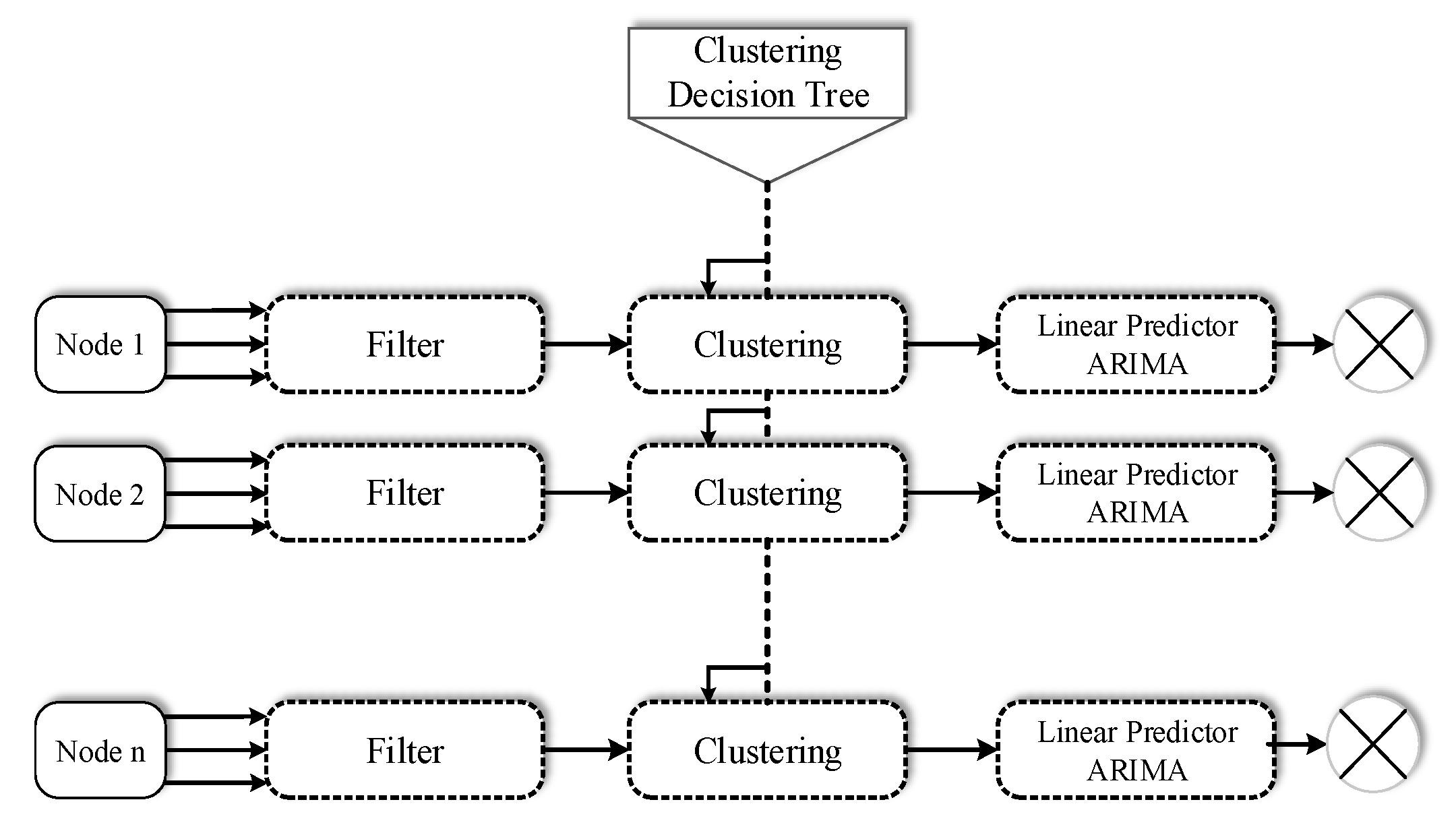
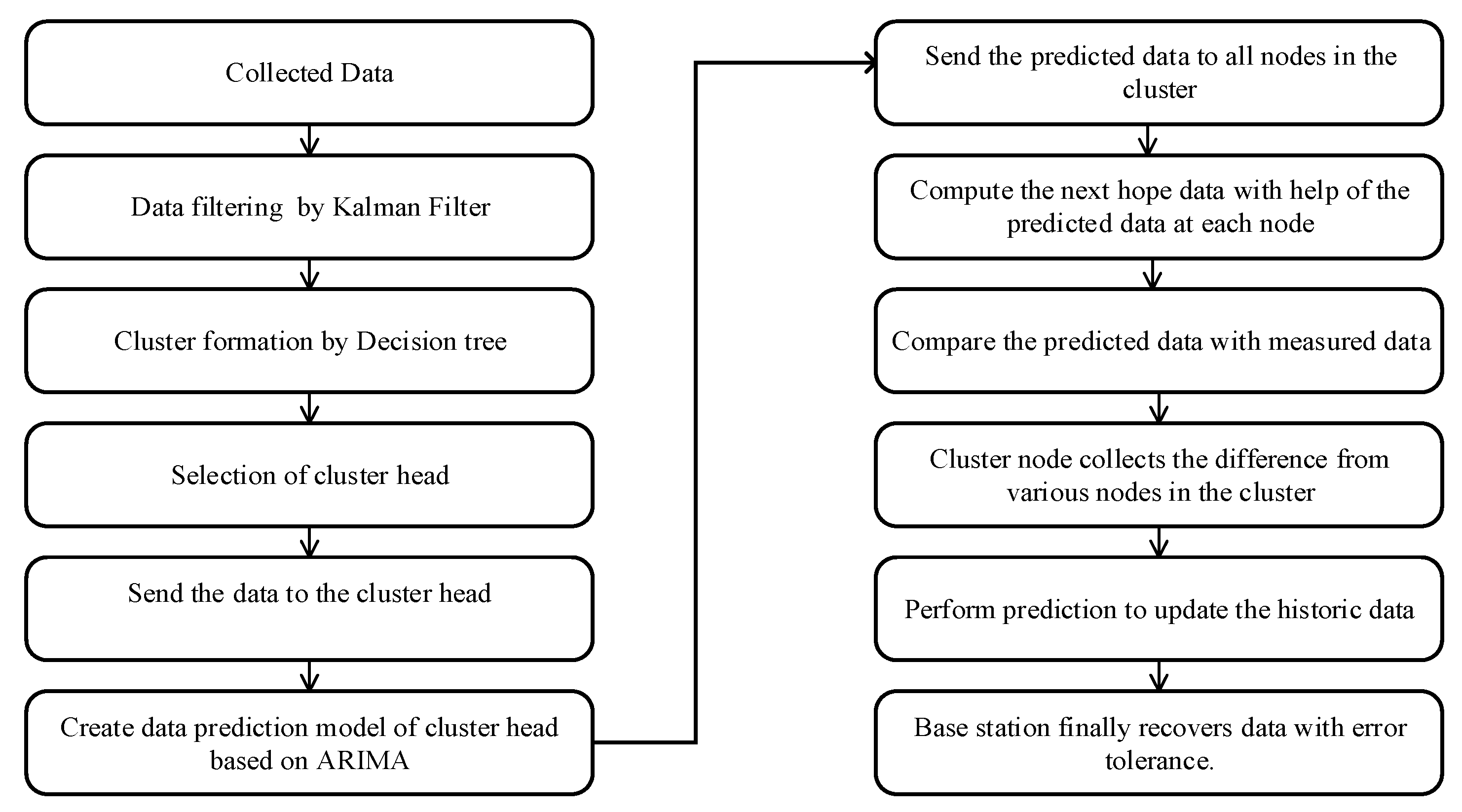
- We designed a model based on decision tree (DT), autoregressive integrated moving average (ARIMA), and Kalman filtering (KF) methods for data prediction in order to reduce unnecessary data transmissions and as a result decrease energy consumption. This model employs a minimal set of sensor nodes for data collection based on intra-cluster prediction and processing of data. In the proposed model, DT is used to filter data associated with each node in order to derive a tree for clustering the sensor data. Additionally, a self-tuning approach based on KF is utilized to optimize estimation while minimizing covariance errors.
- 2
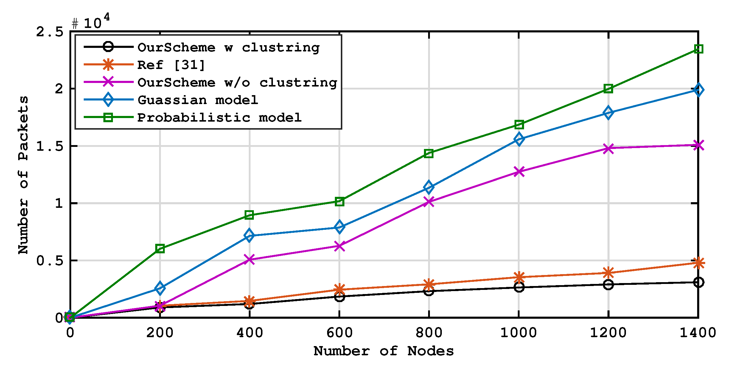
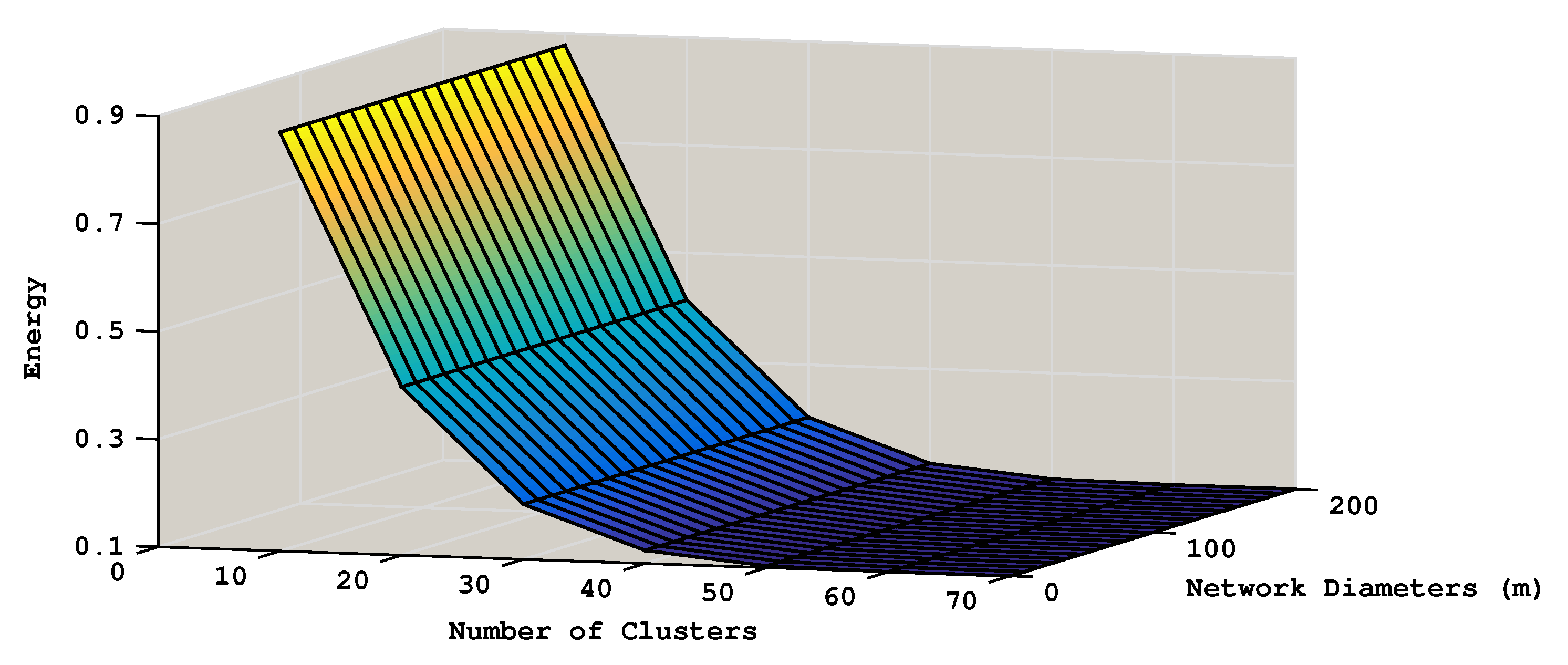
- We provide the MATLAB simulation-based practical demonstration of the proposed model to measure the data packet transmission and energy consumption in sensor nodes under different numbers of distributed sensor nodes in the network.
2. Related Works
3. The Proposed Model
3.1. The Algorithms Employed
- KF is an algorithm that provides estimates of some unknown variables given the measurements observed over time. Kalman filter is used to estimate states based on linear dynamical systems in state-space format. It has a relatively simple form and requires small computational power.
- DT is a popular classification algorithm to understand and interpret. The goal of DT is to create a training model that can be used to predict the class or value of the target variable by learning simple decision rules inferred from prior data.
- ARIMA is an analysis model that uses time series data to predict future trends. It is a hybrid autoregressive model with the moving average model.
3.2. The Hybrid Method
| Algorithm 1: Hybrid algorithm. |
 |
3.3. Adaptive Update of Clustering by DT
3.4. ARIMA Prediction Model
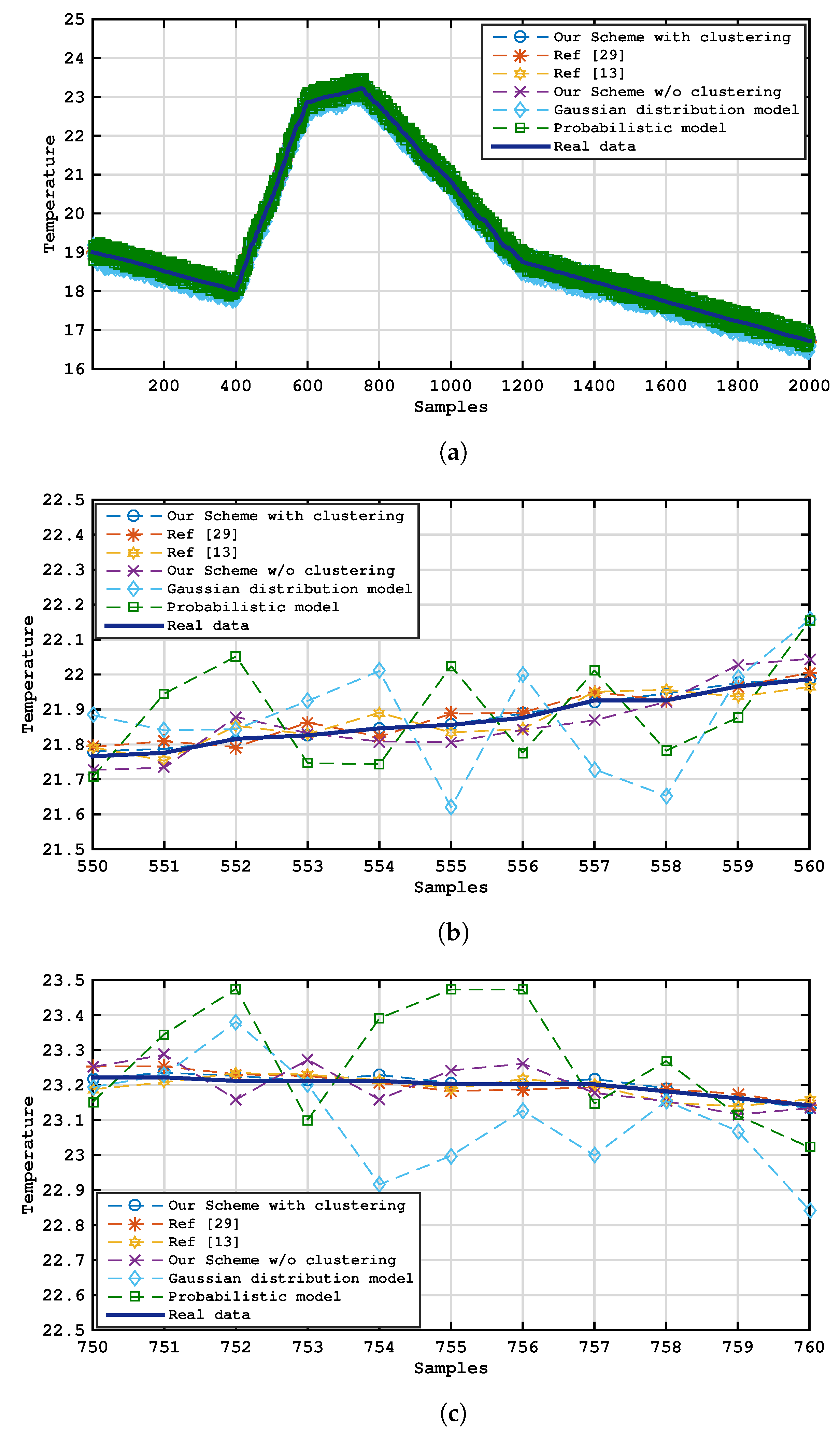
4. Experiment Evaluation and Analysis
5. Conclusions
Author Contributions
Funding
Conflicts of Interest
References
- Arbi, I.B.; Derbel, F.; Strakosch, F. Forecasting methods to reduce energy consumption in WSN. In Proceedings of the 2017 IEEE International Instrumentation and Measurement Technology Conference (I2MTC), Turin, Italy, 22–25 May 2017; pp. 1–6. [Google Scholar]
- Jiang, H.; Jin, S.; Wang, C. Prediction or not? An energy-efficient framework for clustering-based data collection in wireless sensor networks. IEEE Trans. Parallel Distrib. Syst. 2010, 22, 1064–1071. [Google Scholar] [CrossRef]
- Agarwal, A.; Dev, A. A Data Prediction Model Based On Extended Cosine Distance For Maximizing Network Lifetime of WSN. Wseas Trans. Comput. Res. 2019, 7, 23–28. [Google Scholar]
- Tayeh, G.B.; Makhoul, A.; Laiymani, D.; Demerjian, J. A distributed real-time data prediction and adaptive sensing approach for wireless sensor networks. Pervasive Mob. Comput. 2018, 49, 62–75. [Google Scholar] [CrossRef] [Green Version]
- Peksa, J. Prediction Framework with Kalman Filter Algorithm. Information 2020, 11, 358. [Google Scholar] [CrossRef]
- Ferrero, R.; Pegoraro, P.A.; Toscani, S. Synchrophasor Estimation for Three Phase Systems Based on Taylor Extended Kalman Filtering. IEEE Trans. Instrum. Meas. 2020, 69, 6723–6730. [Google Scholar] [CrossRef]
- Zhou, J.; Gu, G.; Chen, X. Distributed Kalman filtering over wireless sensor networks in the presence of data packet drops. IEEE Trans. Autom. Control. 2018, 64, 1603–1610. [Google Scholar] [CrossRef]
- Wang, J.; Zhu, R.; Liu, S. A differentially private unscented Kalman filter for streaming data in IoT. IEEE Access 2018, 6, 6487–6495. [Google Scholar] [CrossRef]
- Pandey, O.J.; Hegde, R.M. Low-latency and energy-balanced data transmission over cognitive small world WSN. IEEE Trans. Veh. Technol. 2018, 67, 7719–7733. [Google Scholar] [CrossRef]
- Yan, R.; Sun, H.; Qian, Y. Energy-aware sensor node design with its application in wireless sensor networks. IEEE Trans. Instrum. Meas. 2013, 62, 1183–1191. [Google Scholar] [CrossRef]
- Goel, S.; Passarella, A.; Imielinski, T. Using buddies to live longer in a boring world [sensor network protocol]. In Proceedings of the Fourth Annual IEEE International Conference on Pervasive Computing and Communications Workshops (PERCOMW’06), Pisa, Italy, 13–17 March 2006; p. 5. [Google Scholar]
- Jang, W.S.; Healy, W.M.; Skibniewski, M.J. Wireless sensor networks as part of a web-based building environmental monitoring system. Autom. Constr. 2008, 17, 729–736. [Google Scholar] [CrossRef]
- Diwakaran, S.; Perumal, B.; Devi, K.V. A cluster prediction model-based data collection for energy efficient wireless sensor network. J. Supercomput. 2019, 75, 3302–3316. [Google Scholar] [CrossRef]
- Xiangning, F.; Yulin, S. Improvement on LEACH protocol of wireless sensor network. In Proceedings of the 2007 International Conference on Sensor Technologies and Applications (SENSORCOMM 2007), Valencia, Spain, 14–20 October 2007; pp. 260–264. [Google Scholar]
- Ouni, S.; Gherairi, S.; Kamoun, F. Data aggregation and pipelining scheduling protocols for real-time wireless sensor networks. Int. J. Hoc Ubiquitous Comput. 2013, 12, 56–64. [Google Scholar] [CrossRef]
- Lavric, A.; Petrariu, A.I.; Coca, E.; Popa, V. LoRa Traffic Generator Based on Software Defined Radio Technology for LoRa Modulation Orthogonality Analysis: Empirical and Experimental Evaluation. Sensors 2020, 20, 4123. [Google Scholar] [CrossRef]
- Ashouri, M.; Yousefi, H.; Basiri, J.; Hemmatyar, A.M.A.; Movaghar, A. PDC: Prediction-based data-aware clustering in wireless sensor networks. J. Parallel Distrib. Comput. 2015, 81, 24–35. [Google Scholar] [CrossRef]
- Sabet, M.; Naji, H. An energy efficient multi-level route-aware clustering algorithm for wireless sensor networks: A self-organized approach. Comput. Electr. Eng. 2016, 56, 399–417. [Google Scholar] [CrossRef]
- Yang, X.; Wen, Y.; Yuan, D.; Zhang, M.; Zhao, H.; Meng, Y. 3-D compression-oriented image content correlation model for wireless visual sensor networks. IEEE Sens. J. 2018, 18, 6461–6471. [Google Scholar] [CrossRef]
- Gedik, B.; Liu, L.; Philip, S.Y. ASAP: An adaptive sampling approach to data collection in sensor networks. IEEE Trans. Parallel Distrib. Syst. 2007, 18, 1766–1783. [Google Scholar] [CrossRef]
- Zhang, D.; Li, G.; Zheng, K.; Ming, X.; Pan, Z.H. An energy-balanced routing method based on forward-aware factor for wireless sensor networks. IEEE Trans. Ind. Inform. 2013, 10, 766–773. [Google Scholar] [CrossRef]
- Shokouhifar, M.; Jalali, A. Optimized sugeno fuzzy clustering algorithm for wireless sensor networks. Eng. Appl. Artif. Intell. 2017, 60, 16–25. [Google Scholar] [CrossRef]
- Olofsson, T.; Ahlen, A.; Gidlund, M. Modeling of the fading statistics of wireless sensor network channels in industrial environments. IEEE Trans. Signal Process. 2016, 64, 3021–3034. [Google Scholar] [CrossRef]
- Imani, M.; Dougherty, E.R.; Braga-Neto, U. Boolean Kalman filter and smoother under model uncertainty. Automatica 2020, 111, 108609. [Google Scholar] [CrossRef]
- Yin, Y.; Shi, J.; Li, Y.; Zhang, P. Cluster head selection using analytical hierarchy process for wireless sensor networks. In Proceedings of the 2006 IEEE 17th International Symposium on Personal, Indoor and Mobile Radio Communications, Helsinki, Finland, 11–14 September 2006; pp. 1–5. [Google Scholar]
- Box, G.E.; Jenkins, G.M.; Reinsel, G.C.; Ljung, G.M. Time Series Analysis: Forecasting and Control; John Wiley & Sons: Hoboken, NJ, USA, 2015. [Google Scholar]
- Madden, S. Intel Lab Data; Intel Research Lab: Berkeley, CA, USA, 2006. [Google Scholar]
- Jiang, H.; Jin, S. Scalable and robust aggregation techniques for extracting statistical information in sensor networks. In Proceedings of the 26th IEEE International Conference on Distributed Computing Systems (ICDCS’06), Lisboa, Portugal, 4–7 July 2006; p. 69. [Google Scholar]
- Wu, M.; Tan, L.; Xiong, N. Data prediction, compression, and recovery in clustered wireless sensor networks for environmental monitoring applications. Inf. Sci. 2016, 329, 800–818. [Google Scholar] [CrossRef]
- Chu, D.; Deshpande, A.; Hellerstein, J.M.; Hong, W. Approximate data collection in sensor networks using probabilistic models. In Proceedings of the 22nd International Conference on Data Engineering (ICDE’06), Atlanta, GA, USA, 3–7 April 2006; p. 48. [Google Scholar]
- Pala, Z. Effects of Mica2-based discrete energy levels on the lifetime of cooperation neighbor sensor networks. Turk. J. Electr. Eng. Comput. Sci. 2016, 24, 2671–2678. [Google Scholar] [CrossRef]
- Barak, S.; Sadegh, S.S. Forecasting energy consumption using ensemble ARIMA—ANFIS hybrid algorithm. Int. J. Electr. Power Energy Syst. 2016, 82, 92–104. [Google Scholar] [CrossRef] [Green Version]


| ARIMA | Coefficients | St. Dev. |
|---|---|---|
| AR (1) | −0.7144 | 7.0748 |
| AR (2) | −0.4466 | 4.0677 |
| AR (3) | 1.2873 | 5.0433 |
| AR (1) | −0.7144 | 7.0748 |
| AR (2) | −0.4466 | 4.0677 |
| AR (3) | 1.2873 | 5.0433 |
| AR (1) | 0.1765 | 4.753 |
| AR (2) | 0.1106 | 4.043 |
| AR (3) | 0.1076 | 7.753 |
| MA (1) | −0.4131 | 7.0293 |
| MA (2) | 1.7011 | 5.0988 |
| MA (3) | −0.1510 | 5.0728 |
| MA (1) | 0.4355 | 7.0981 |
| MA (2) | 1.2788 | 5.1067 |
| MA (3) | 0.1314 | 4.0433 |
| MA (1) | −0.3081 | 6.233 |
| MA (2) | 0.2944 | 4.053 |
| MA (3) | 0.8733 | 5.012 |
| Number of Nodes | |||
|---|---|---|---|
| 500 | 1000 | 1500 | |
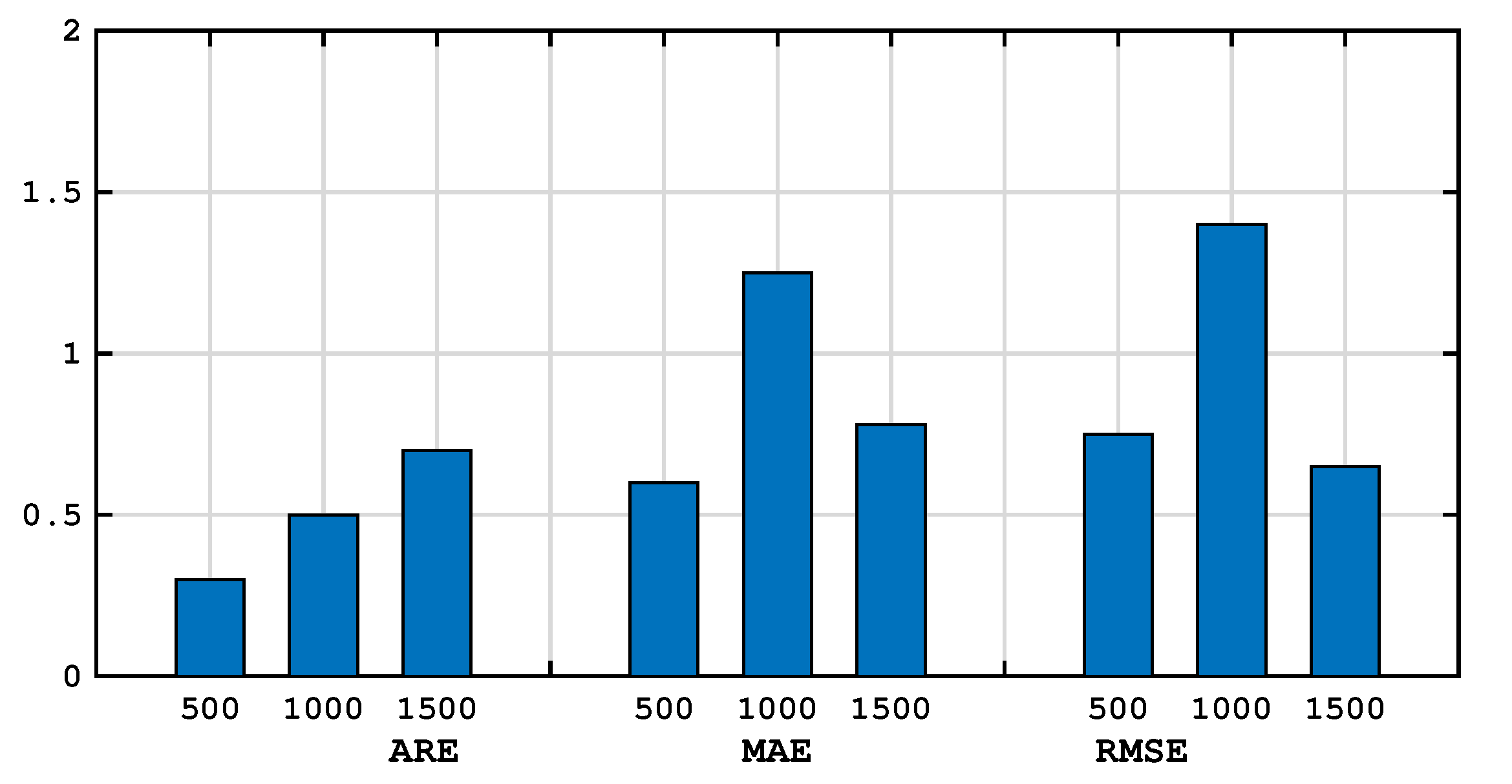
| ARE | 0.4 | 4.5 | 5.5 |
| MAE | 0.5 | 1.05 | 0.55 |
| RMSE | 0.8 | 1.2 | 0.52 |
Publisher’s Note: MDPI stays neutral with regard to jurisdictional claims in published maps and institutional affiliations. |
© 2020 by the authors. Licensee MDPI, Basel, Switzerland. This article is an open access article distributed under the terms and conditions of the Creative Commons Attribution (CC BY) license (http://creativecommons.org/licenses/by/4.0/).
Share and Cite
Soleymani, S.A.; Goudarzi, S.; Kama, N.; Adli Ismail, S.; Ali, M.; MD Zainal, Z.; Zareei, M. A Hybrid Prediction Model for Energy-Efficient Data Collection in Wireless Sensor Networks. Symmetry 2020, 12, 2024. https://doi.org/10.3390/sym12122024
Soleymani SA, Goudarzi S, Kama N, Adli Ismail S, Ali M, MD Zainal Z, Zareei M. A Hybrid Prediction Model for Energy-Efficient Data Collection in Wireless Sensor Networks. Symmetry. 2020; 12(12):2024. https://doi.org/10.3390/sym12122024
Chicago/Turabian StyleSoleymani, Seyed Ahmad, Shidrokh Goudarzi, Nazri Kama, Saiful Adli Ismail, Mazlan Ali, Zaini MD Zainal, and Mahdi Zareei. 2020. "A Hybrid Prediction Model for Energy-Efficient Data Collection in Wireless Sensor Networks" Symmetry 12, no. 12: 2024. https://doi.org/10.3390/sym12122024