Train Regulation Combined with Passenger Control Model Based on Approximate Dynamic Programming

Abstract

Rescheduling is often needed when trains stay in segments or stations longer than specified in the timetable due to disturbances. Under crowded situations, it is more challenging to return to normal with heavy passenger flow. Considering making a trade-off between passenger loss and operating costs, we present a train regulation combined with a passenger control model by analyzing the interactive relationship between passenger behaviors and train operation. In this paper, we convert the problem into a Markov decision process and then propose the management strategy of regulating the running time and controlling the number of boarding passengers. Owing to the high dimensions of the large-scale problem, we applied the Approximate Dynamic Programming (ADP) approach, which approximates the value function with state features to improve computational efficiency. Finally, we designed three experimental scenarios to verify the effectiveness of our proposed model and approach. The results show that both the proposed model and the approach have a good performance in the cases with different passenger flows and different disturbances.

1. Introduction

When operation suffers a disturbance, prompt rescheduling measures must be taken to maintain the robustness of the metro system. In the past few years, train rescheduling has caused great concerns among many researchers, and many different approaches have been developed with different model formulations.

In some studies, the train rescheduling problem is converted into the problem of mathematical programming, aiming to make the operation return to normal as soon as possible by altering the running time and dwelling time. Usually, it is most important to maintain service as much as possible for the customers [1]. In early work, classical optimization methods were used for rail transit train regulation to describe passenger perception of service quality [2]. In the study by D’riano [3], train scheduling was viewed as a job shop scheduling problem with no-store constraints and was modeled with the alternative graph formulation. The branch-and-bound algorithm was used in this to obtain the optimization solution. A mixed integer programming model was established in Ref. [4] to minimize the incidents’ impact with a heuristic algorithm. There have been some studies on train regulation problems with high nonlinearity, heavy constraints, and stochastic characteristics, such as Ref. [5]. Besides, some efficient train operation control algorithms were presented in Refs. [6,7] with the highly increasing concerns about environmental protection.

In another type of research, the train rescheduling model has been established based on discrete event dynamic systems theory. The discrete-time traffic system was described earlier in Ref. [8], and this study used state feedback control algorithms to optimize system performance and ensure system stability. Then, a discrete event model was adopted to handle perturbations in the railway network [9]. Recently, discrete methods have received more attention. In Ref. [10], the subway line was characterized through the train positions’ state transition on the basis of discrete events. A timed colored Petri network was adopted in Ref. [11] to describe the railway system with double-track lines. The Markov decision framework was proposed to deal with the uncertain disturbances in real-time train operation by Yin et al. [12].

Currently, the headway between trains has become smaller with the growing passenger demand, which raises higher requirements for train rescheduling. To improve the computational efficiency, many techniques have been tried. A general genetic algorithm was applied in Ref. [13] to get the train optimization solutions. For the same problem, a heuristic greedy approach that performs a depth-first search that branches according to a set of criteria was described by Krasemann [14]. The Problem Space Search (PSS) meta-heuristic was used in Ref. [15] for large-scale problems to generate a revised timetable quickly. In Ref. [6], approximate dynamic programming was proposed to solve the stochastic programming and obtain a high-quality solution within a short time compared with the MIP solver. Based on a standard event-based MILP formulation in Ref. [16], the solution was addressed by an ad-hoc heuristic preprocessing on top of a general-purpose commercial solver.

With high-frequency operation and high traffic density, the metro system now is more sensitive to disturbances and more unstable than the traditional system. During rush hour, passenger demand is high, even exceeding the transportation capacity, so that the dwelling time is often extended by squeezing in passengers, leading to a departure delay. Although the metro system is commonly equipped with ATC (Automatic Train Control), enabling making an adjustment to improve the punctuality by altering the travel speed profile, it has a limited responsiveness to the dynamics of passenger flow and unloading the gathered passengers. Therefore, train operation combined with demand management is needed in practice.

In this context, a joint optimal train regulation and passenger flow control model was first developed by Li et al. [17] aiming to improve the headway regularity and commercial speed under perturbations, based on the assumption that the dwelling time of each train is affected by boarding and alighting passengers. The paper defined a state vector that consists of operation error and passenger loading error to describe the linear time-varying system. In order to minimize the system error, train regulation and the passenger control measure are adopted jointly to adjust the running time and dwelling time. The simplified joint dynamic model described the evolution of the departure time and the passenger loading in the form of a matrix. However, the formulation cannot reflect some feature variables, such as the number of passengers left on the platform. It also ignored the total delay of passengers, which is one of the important performances of the rescheduling problems. In addition, the proposed model is only applicable to slight delays in a certain range.

Therefore, considering minimizing the total delay of passengers and service quality, as well as adjustment costs under dynamic passenger flow, we propose train regulation combined with a passenger control model under discrete the Markov decision process framework. Moreover, we take the uncertainty in the dwelling process into account. Similarly, the running time and the number of passengers’ control are selected as two variables in our study.

In principle, the Markov decision problem can be solved by using dynamic programming algorithms, such as value iteration and policy iteration [18]. However, the rescheduling problem is high-dimensional, involving a large number of variables, which render such an algorithm infeasible. To address the problem, Approximate Dynamic Programming (ADP) is applied in our paper. ADP was development by Powell to overcome the curse of dimensionality [19]. The method has been widely applied in various sequential stochastic optimization problems, such as the network capacity control problem in Ref. [20], supply risk management in Ref. [21], and transshipment policy optimization in Ref. [22]. In our study and experiments, the dynamic operation of the metro system is described explicitly through the Markov decision model, and the ADP method helps us lower the dimensions of the variables. With different scenario settings, the experiments’ results demonstrate the fast convergence performance in the case of a large-scale problem.

The rest of this paper is organized into several parts. In Section 2, we first state the problem and give the assumptions of the study. Then, in Section 3, we present our train adjustment model based on the analysis of the interaction of train operation and dynamic passenger flow. In Section 4, we explain the ADP algorithm’s superiority and the algorithm procedure. In Section 5, three experimental scenarios are implemented to verify the validity of the proposed model and algorithm. Finally, some improvements and future works are put forward in the Conclusion section.

2. Problem Description

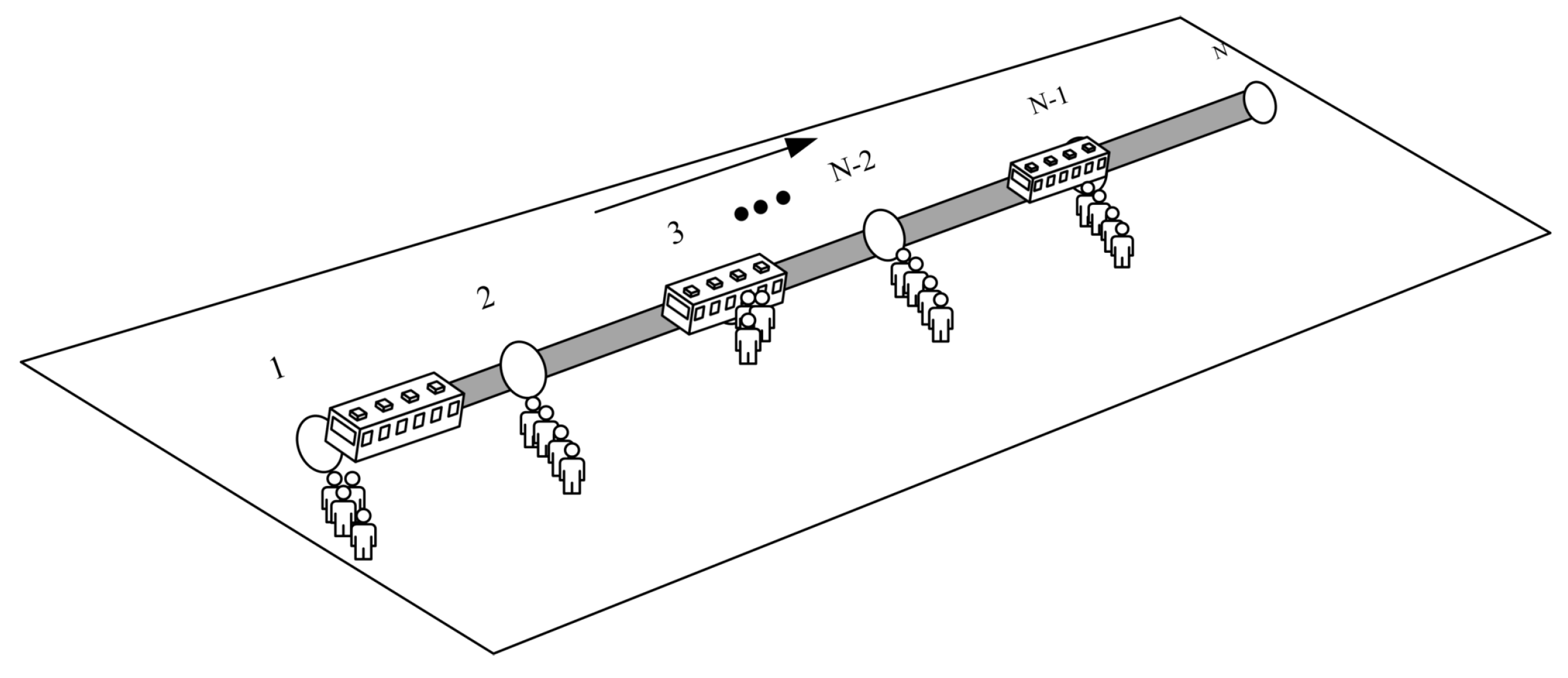
This paper considers a singe-track metro with N stations and $N-1$ running sections. As shown in Figure 1, each train begins its journey from the first station and dwells at the station for a period, waiting for passengers’ alighting and boarding in sequence, then arrives at the next station by running in a section according to a given train timetable. To make the study easy to understand, we give the variable notations of the train service process in

Table 1. Notations.

Symbol	Definition
$i=1,2,...,M$	indices of the trains on the line;
$j=1,2,...,N$	indices of the stations on the line;
$D_{i,j}$	the normal dwelling time of the ith train at the jth station;
$U_{i,j}$	the normal section running time of the ith train from the jth station to the $(j+1)$th station;
$U_{i,j}^{min}$	the minimum running time of the ith train from the jth station to the $(j+1)$th station;
$U_{i,j}^{max}$	the maximum running time of the ith train from the jth station to the $(j+1)$th station;
$t_{i,j}$	the actual arrival time of the ith train at the jth station;
$s_{i,j}$	the actual dwelling time of the ith train at the jth station;
$s_{i,j}^{max}$	the maximum dwelling time of the ith train at the jth station;
$s_{i,j}^{min}$	the minimum dwelling time for opening and closing the doors;
$H^{max}$	the maximum headway of the two consecutive trains;
$H^{min}$	the minimum headway of the two consecutive trains;
$m_{i,j}$	the number of boarding passengers for train i at station j;
$n_{i,j}$	the number of alighting passengers for train i at station j;
$l_{i,j}$	the number of in-vehicle passengers when train i arrives at station j;
$w_{i,j}$	the number of waiting passengers on the platform when train i arrives at station j;
$d_{i,j}$	the arrival delay of train i at station j;
${\lambda }_{i,j}$	passenger arrival rate between the arrival of train $i-1$ and train i at station j.
Decision variables	Definition
$u_{i,j}$	the actual running time of train i for section j;
$p_{i,j}$	the number of controlled passengers of train i for section j.

.

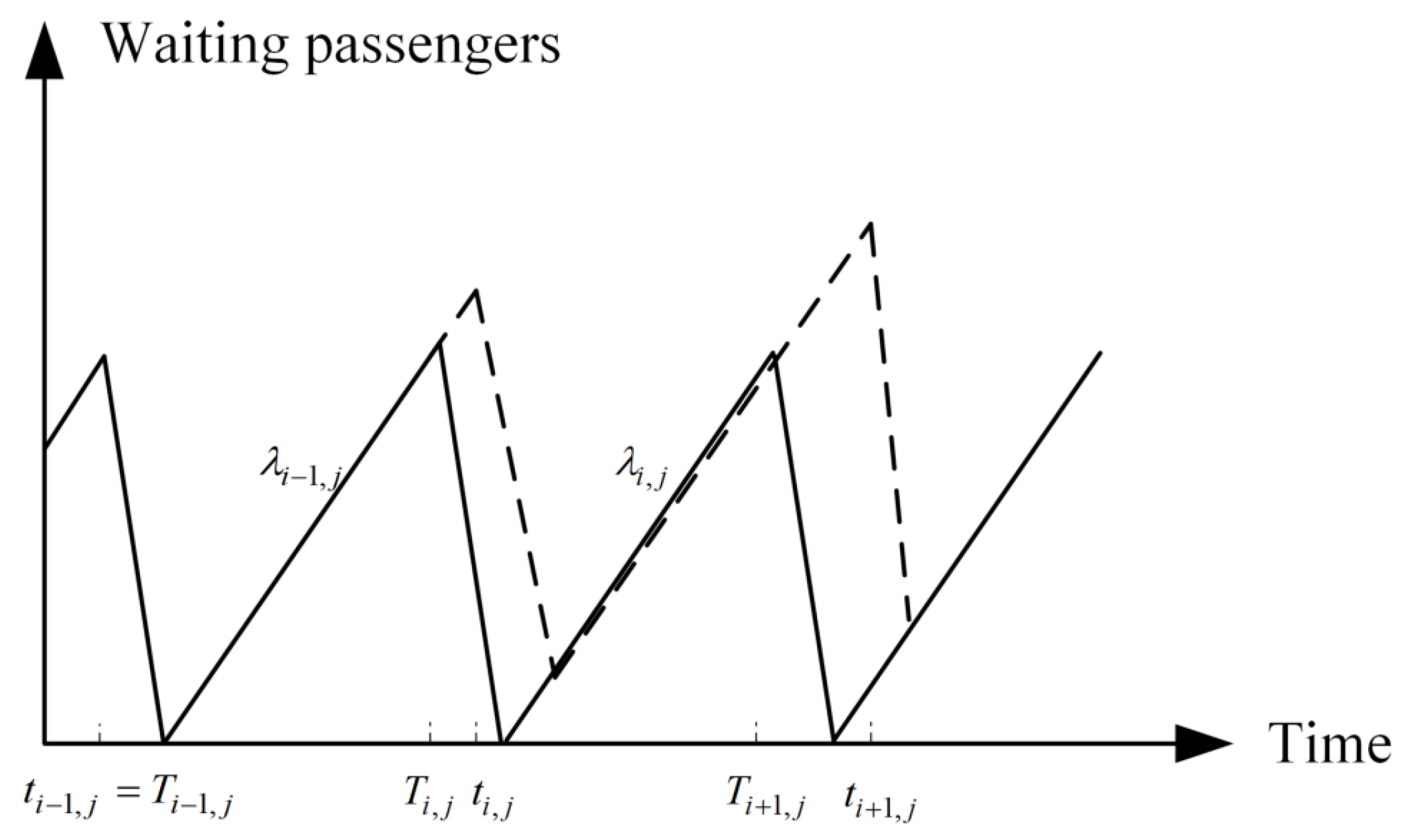
Generally, passengers are delivered from the origin to their destination as they expect. However, it is inevitable that trains will suffer disturbances and that the operation will deviate from the pre-determined timetable in the actual operation. In the cruising phase, equipment failure, improper driving behavior, or sudden accidents can cause a late arrival. In the loading process, there are also some uncertainties that can result in a departure delay, for instance the passengers in the train are so crowded, that the door cannot be closed on time. If the deviation of the operation is not eliminated in time, the delay could propagate throughout the network due to the cumulative passengers, which has been simulated in Refs. [23,24]. The fluctuation of waiting passengers on the platform is illustrated in Figure 2. To prevent a second delay, train rescheduling is necessary.

Usually, both dwelling time and running time would be reset in a train rescheduling problem. However, with the fast-growing passenger demand, the recovery of train operation experiences more difficulty. Once a delay occurs, more passengers will accumulate in a short time with the originally huge arriving passenger flow. This requires higher transportation efficiency and sufficient dwelling time to disperse passengers, otherwise more passengers will be retained and more trains will deviate from the previous schedule, thus influencing the operational efficiency of the entire network. Besides, the squeezing in of passengers increases the uncertainty of the dwelling process, as well; while the delayed train needs to depart as soon as possible to improve its punctuality performance at a later station. Therefore, a passenger control measure should be taken to regulate the dwelling time, thereby achieving a trade-off between the number of loaded passengers and the time required to return to the normal condition.

In addition, inappropriate running regulation strategies may be counterproductive with lower service quality and higher operating costs as well. According to Ref. [25], a smaller section running time leads to a greater energy consumption. In addition, excessive acceleration to move faster would cause passenger discomfort. As for the adjustment of dwelling time, it also should integrate the train dispatching and passenger loading.

To develop an adjustment model, we first discuss the interaction between passenger flow and train operation. In reality, the start and end of the train service are part of the process of train stopping. The dwelling time is usually predetermined, which matches with passenger flow in the timetabling stage. However, it should be reset in the case of disturbances in order to return to the original timetable. Therefore, in this paper, we consider determining the dwelling time based on passenger flow, which has been investigated greatly in Refs. [26,27]. According to Ref. [28], dwelling time was considered to be closely related to the speed at which passengers move and the crowding degree, as the following formulation.

$$s_{i,j}={\beta }_0+{\beta }_1{n}_{i,j}+{\beta }_2{m}_{i,j}+{\beta }_3{(w_{i,j}/n^{door})}^3{m}_{i,j}.$$

(1)

$$n_{i,j}={\mu }_{i,j}{l}_{i,j}$$

(2)

where ${\beta }_0,{\beta }_1,{\beta }_2,{\beta }_3$ are given correlation coefficients, which can be estimated according to historical data. $n^{door}$ is the number of doors of the vehicle. In this paper, the difference of the number of waiting passengers before doors is neglected, and we assume that the number of alighting passengers is proportional to the number of passengers in the vehicle, with the ratio set as ${\mu }_{i,j}$.

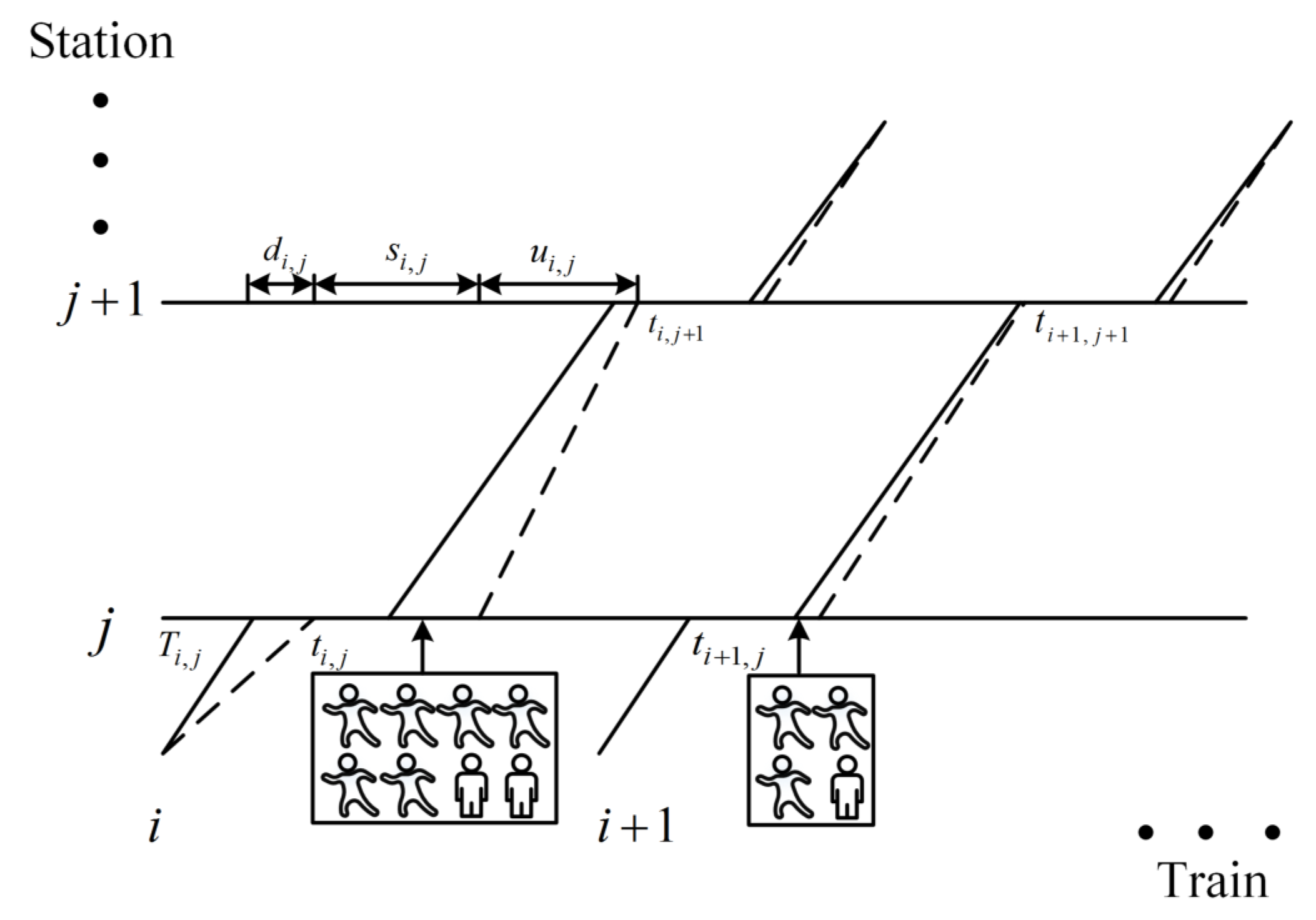
As Figure 3 shows, after the train’s arrival at a station, the arrival at the next station is only determined by the dwelling time in the former station and the section running time, being the initial stage of the later schedule. Accordingly, based on the interactive process of passenger boarding and train operation, we propose a train regulation combined with a passenger control model to restore the deviation of the train operation to a reasonable range as soon as possible concerning both the passengers and operation costs.

Ahead of the model formulation, we give several assumptions as follows. (1) To simplify the problem, skip-stopping and overtaking are not permitted in our study, so the order of the train passing through the station is determined. (2) We do not consider the impact of the passenger control measure on the passenger demand. This means that the passenger would not leave the station or reroute in spite of being denied. (3) In peak hours, the number of passengers entering stations fluctuates a little in general, so we used the passenger arrival rate obtained through ATC data directly, ignoring the temporal gap between the moment passengers enter the station and their arrival at the platform.

3. Model Establishment

As illustrated in Figure 1, train operation planning is a multi-stage decision problem involving passenger flow. When a train departs from a station, the arrival time depends on the running time. Based on the dwelling model we discussed before, the number of boarding passengers subject to remaining capacity determines the dwelling time and the departure time. There will be some passengers on left platform if the volume is not sufficient. If we consider the period from one departure to another departure as a step, the metro system evolves in such a discrete stage. Therefore, from the planning level, we convert the train rescheduling problem into a Markov decision process. The formulations are as follows.

State, ${\mathit{S}}_{i,j}$, is a vector that is made from the arrival time of the train, the number of passengers in the vehicle, the number of waiting passengers, and the delay of the arrival time.

$${\mathit{S}}_{i,j}=(t_{i,j},l_{i,j},w_{i,j},d_{i,j}).$$

(3)

Action, ${\mathit{x}}_{i,j}$, are decision variables at each step, denoted as Equation (4), which we mentioned previously.

$${\mathit{x}}_{i,j}=(p_{i,j},u_{i,j}).$$

(4)

where $p_{i,j}$ also equals the number of remaining passengers who are left at the platform to wait for the next train.

State transfer function indicates how the state ${\mathit{S}}_{i,j}$ evolves to the state ${\mathit{S}}_{i,j+1}$ exposed to the action ${\mathit{x}}_{i,j}$. The function is expressed as Equation (5), and the components of the state vector can be obtained by Equations (7)–(10).

$${\mathit{S}}_{i,j}=S^M({\mathit{S}}_{i,j},{\mathit{x}}_{i,j}).$$

(5)

$$m_{i,j}=w_{i,j}-n^{door}{p}_{i,j}$$

(6)

$$t_{i,j+1}=t_{i,j}+s_{i,j}+u_{i,j}$$

(7)

$$l_{i,j+1}=l_{i,j}+w_{i,j}-n^{door}{p}_{i,j}-n_{i,j}.$$

(8)

$$w_{i,j+1}={\int }_{t_{i-1,j+1}}^{t_{i,j+1}}{\lambda }_{i,j+1}dt+n^{door}{p}_{i-1,j+1}.$$

(9)

$$d_{i,j+1}=t_{i,j+1}-T_{i,j}.$$

(10)

Immediate cost, $c_{i,j}$, generated by action ${\mathit{x}}_{i,j}$, is formulated by:

$$c({\mathit{S}}_{i,j},{\mathit{x}}_{i,j})=w_d{d}_{i,j}·w_{i,j}+w_p{p}_{i,j}^2+w_e{(u_{i,j}-U_{i,j})}^2$$

(11)

where, $w_d$, $w_p$, and $w_e$ are weighted parameters. In the problem of this paper, we aim to minimize the total delay of all the disturbed trains with minimal impact on both operation costs and service quality. Therefore, the three terms make up the decision cost in our model. The first one is the total delay of passengers. The second is added to penalize the passenger control to reduce the negative impact on service quality. The third term is the train regulation penalty. As we discussed before, the variance of running time should be kept small considering less extra energy consumption and small acceleration change to avoid passenger discomfort.

However, in fact, train adjustment is a real-time problem, and the number of affected trains is unknown, but depends on our policy. We can only predict the future based on the current status and the information we have. In MDP, the value function is calculated to judge how good the decision is in each step. For state ${\mathit{S}}_{i,j}$, it is formulated with the long-term expected return, and then, the recursion formula is described as Equation (12) according to the Bellman optimality principle.

$$v_{i,j}\left({\mathit{S}}_{i,j}\right)=c({\mathit{S}}_{i,j},{\mathit{x}}_{i,j})+\gamma \sum _{{\mathit{S}}^{{}^{\prime }}\in \mathbf{S}}P\left({\mathit{S}}^{{}^{\prime }}\right|{\mathit{S}}_{i,j})V_{i,j+1}\left({\mathit{S}}^{{}^{\prime }}\right).$$

(12)

where $\gamma$ is the discount factor, which indicates the impact of current actions on future ones. $\mathit{S}$ is the set of allpossible states.

In actual operation, the train operation is also subject to the following constraints on the operating environment and safety restrictions.

$$U_{i,j}^{min}\le u_{i,j}\le U_{i,j}^{max}$$

(13)

$$s_{i,j}^{min}\le s_{i,j}\le s_{i,j}^{max}$$

(14)

$$0\le p_{i,j}\le w_{i,j}/n^{door}$$

(15)

$$H^{min}\le t_{i,j}-t_{i-1,j}\le H^{max}$$

(16)

$$t_{i,j}\ge T_{i,j}$$

(17)

$$l_{i,j}\le \sigma C$$

(18)

where Equations (13)–(18) are the section running time constraint, dwelling time constraint, passenger control constraint, headway constraint, and passenger loading constraint. C is the vehicle loading capacity, and $\sigma$ is the overload ratio.

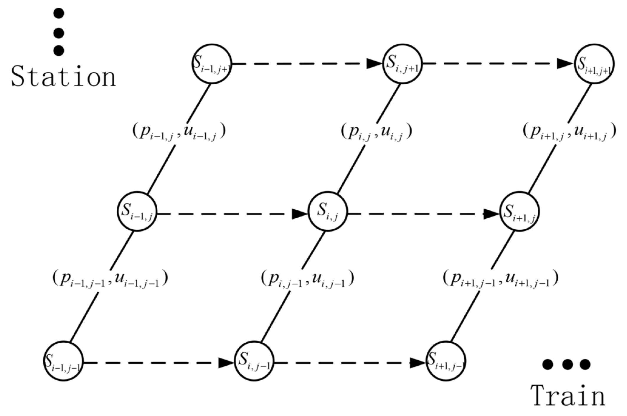
The decision-making process of the proposed model can be explained explicitly by Figure 4. For train i at station j, ${\mathit{S}}_{i,j-1}$ is the past state, and ${\mathit{S}}_{i,j}$ is the current state. After making a decision ${\mathit{x}}_{i,j}$, which are the number of passenger control and section running time based on the current state, train i moves to station $j+1$ and ${\mathit{S}}_{i,j}$ transfers to the next ${\mathit{S}}_{i,j+1}$; an immediate cost $c_{i,j}$ is produced simultaneously.

4. Approximation Dynamic Programming Method

4.1. Algorithm Idea

In deterministic dynamic programming, the strategy of backward search needs to sweep and calculate all feasible states and action spaces at the cost of huge computational time and storage. For large-scale problems with numerous states and actions, the dimension increases exponentially, making the decision process intractable.

ADP offers a powerful tool for seeking the optimal policy and can effectively address the problem of dimensional explosion. To avoid this bootstrapping, it approximates the value function and steps forward in time, then iteratively updates the approximated function targeting the minimum estimation error until convergence. Virtually, the process of approaching the optimal solution continually is finite loops that contain value function approximation, decision-making, state transition, and value function update. The value function approximation and update are two main strategies that affect the accuracy of the method.

Notice that the value function composes immediate cost and the value function of the next state. In the ADP method, the post-decision state is introduced to capture the state of the system immediately after decision-making, but before the arrival of new information. According to:

$${\mathit{S}}_{i,j}^x=S^{M,x}({\mathit{S}}_{i,j},{\mathit{x}}_{i,j}),$$

(19)

Equation (12) is rewritten as:

$$v_{i,j}\left({\mathit{S}}_{i,j}\right)=min[c({\mathit{S}}_{i,j},{\mathit{x}}_{i,j})+V_{i,j}\left({\mathit{S}}_{i,j}^x\right)].$$

(20)

According to Ref. [19], there are many techniques to approximate the value function. The basic function is one of the popular methods to create the approximation function through the features of the state variables, as it is easy to work with. Additionally, it will work well for discrete scheduling problems and offer computational advantages with regards to algorithms for computing appropriate parameters. To formulate the basic function, we recombined the four kinds of attributes in the state vector to extract the following features: Feature 1: $t_{i,j}$, the arrival time of trains, the most intuitive characteristic of the train rescheduling problem. Feature 2: $l_{i,j}·d_{i,j}$, the total delay of the passengers in the vehicle. Feature 3: $w_{i,j}·d_{i,j}$, the total delay of the waiting passengers.

Compared with nonlinear approximation, linear approximation has only one optimal value and can converge to the global optimum. Therefore, we approximate the value function with the form of Equation (21).

$$V_{i,j}\left({\mathit{S}}_{i,j}^x\right)\approx {\overline{\mathit{V}}}_{i,j}\left({\mathit{S}}_{i,j}\right)=\sum _{f\in \varphi }{\mathit{\theta }}_f{\varphi }_f\left({\mathit{S}}_{i,j}^x\right)$$

(21)

where ${\mathit{\theta }}_f$ is the weight parameter vector and ${\varphi }_f$ are the basic functions above. Thereby, the value function is:

$${\tilde{v}}_{i,j}^{*}\left({\mathit{S}}_{i,j}\right)=min[c({\mathit{S}}_{i,j},{\mathit{x}}_{i,j})+{\overline{V}}_{i,j}\left({\mathit{S}}_{i,j}^x\right)]$$

(22)

Note that the value function of final state is set to zero.

In each decision time, we use a pure exploration strategy to select the current optimal decision as Equation (23). Though the approximate value function is not the optimal one in the iteration, we use it a to make decisions; because in ADP, the special idea of computing the value function is to find decisions that can balance the cost now with the costs in the future instead of getting the optimal value once.

Given an approximation, a suboptimal decision can be generated using:

$${\mathit{x}}_{i,j}^{*}=arg\left[{\tilde{v}}_{i,j}^{*}\left({\mathit{S}}_{i,j}\right)\right].$$

(23)

Now, we turn to the parameter update problem. The approximate function means that the value function ${\overline{V}}_{i,j}\left({\mathit{S}}_{i,j}\right)$ depends entirely on vector ${\mathit{\theta }}_f$ and only changes with ${\mathit{\theta }}_f$ at different decision stages. The approximate value function strategy is to approach the true value infinitely by updating ${\mathit{\theta }}_f$, reducing the error between the estimated value and the true value to be as small as possible. Therefore, the mean squared error can be used as the performance function approximation criterion.

$$\begin{array}{c}\hfill MSE{\left({\mathit{\theta }}_f\right)}^{*}=\sum _{S\in \mathcal{S}}{P}_{\mathcal{S}}{[V_{i,j}\left({\mathit{S}}_{i,j}\right)-{\overline{V}}_{i,j}\left({\mathit{S}}_{i,j}\right)]}^2.\end{array}$$

(24)

$$\begin{array}{c}\hfill MSE{\left({\mathit{\theta }}_f\right)}^{*}=\sum _{S\in \mathcal{S}}{P}_{\mathcal{S}}{[v_{i,j}\left({\mathit{S}}_{i,j}\right)-{\tilde{v}}_{i,j}\left({\mathit{S}}_{i,j}\right)]}^2.\end{array}$$

(25)

Since all possible states have the same distribution, the gradient direction is the direction with the fastest decrease in error for Equation (25). In each iteration, the parameter vector gets updated along this direction.

$${\mathit{\theta }}_{i,j}^n={\mathit{\theta }}_{i,j}^{n-1}+\frac{1}{2}{\alpha }_{n-1}[v_{i,j}\left({\mathit{S}}_{i,j}\right)-{\tilde{v}}_{i,j}\left({\mathit{S}}_{i,j}\right)]{\nabla }_{{\mathit{\theta }}_{i,j}^{n-1}}{\tilde{v}}_{i,j}^n\left({\mathit{S}}_{i,j}\right)$$

(26)

where ${\alpha }_n$ is the step of the gradient algorithm. Notice that in Equation (26), the real value $v_{i,j}\left({\mathit{S}}_{i,j}\right)$ is unknown. To ensure the update, we borrow temporal-difference prediction methods in reinforcement learning [29], replacing the real value with the expected TD target. It has the advantage of being model-free, learning by bootstrapping from the current estimate of the value function. The difference between the estimated value of the state and the better estimated return is measured by TD error ${\delta }_n$.

$${\delta }_n=c({\mathit{S}}_{i,j},{\mathit{x}}_{i,j})+\gamma {\tilde{v}}_{i,j+1}^{n-1}\left({\mathit{S}}_{i,j+1}\right)-{\tilde{v}}_{i,j}^{n-1}\left({\mathit{S}}_{i,j}\right)$$

(27)

Finally, the weight vector is updated by:

$${\mathit{\theta }}_{i,j}^n={\mathit{\theta }}_{i,j}^{n-1}+\alpha {\delta }_n\nabla {\tilde{v}}_{i,j}^n\left(\mathit{S}\right).$$

(28)

4.2. Algorithm Procedure

According to the formulated Markov decision problem, the main algorithm of the train regulation combined with a passenger control model is described as follows.

First, the initial state is built with ${\mathit{S}}_{\tilde{i},\tilde{j}}$, including the delay and the passenger information. The regulation starts with the initial state until all trains’ operation is restored to the scheduled one. For a given iteration n and the current state ${\mathit{S}}_{i,j}$, the optimal action ${\mathit{x}}_{i,j}$ is selected by Equation (23) by sweeping all the actions in the feasible set determined by the operation constraints and calculating the expected value after taking the action. Thus, the current state ${\mathit{S}}_{i,j}$ transfers to the next state ${\mathit{S}}_{i,j+1}$ by the state transfer function (5), which will be viewed as the current state in the next decision step. After finishing the decision of all the stages, we get a sample path $[({\mathit{S}}_{\tilde{i},\tilde{j}},{\mathit{x}}_{\tilde{i},\tilde{j}}),({\mathit{S}}_{\tilde{i},\tilde{j}+1},{\mathit{x}}_{\tilde{i},\tilde{j}+1}),\cdots ,({\mathit{S}}_{i,j},{\mathit{x}}_{i,j}),\cdots ,({\mathit{S}}_{i+1,j},{\mathit{x}}_{i+1,j}),\cdots ,({\mathit{S}}_{K,N-1},{\mathit{x}}_{K,N-1}),({\mathit{S}}_{K,N},{\mathit{x}}_{K,N})]$, which corresponds to a policy. Next, update all the approximated function coefficients ${\mathit{\theta }}_f$, and substitute the approximate function for the next iteration based on the policy value function. Repeat the same steps until the maximal iteration time or iterate result converges. The detailed algorithm procedure is presented in Algorithm 1 below.

Algorithm 1 Algorithm procedure.

Input:  initial delay state and algorithm parameters 1: set ${\mathit{\theta }}_{i,j}=\mathbf{0},{\delta }^n=0,v_{i,j}^0\left({\mathit{S}}_{i,j}\right)=0$ 2: set $n=1$ 3: while$n\le N$do 4:  for $i\in ı$ do 5:   for $j\in j$ do 6:    if ${\mathit{S}}_{i,j}$ is final state then 7:     ${\tilde{v}}_{i,j}^n=0$ 8:    else 9:     ${\tilde{v}}_{i,j}^n=min(c({\mathit{S}}_{i,j},{\mathit{x}}_{i,j})+\gamma {\overline{V}}_{i,j}^x\left({\mathit{S}}_{i,j}\right))$ 10:     Pure exploration strategy: ${\mathit{x}}_{i,j}^{*}=\mathrm{argmin}{\tilde{v}}_{i,j}^n$ 11:     State transfer: ${\mathit{S}}_{i,j+1}\leftarrow S^M({\mathit{S}}_{i,j},{\mathit{x}}_{i,j})$ 12:    end if 13:   end for 14:  end for 15:  Update TD error ${\delta }^n=c({\mathit{S}}_{i,j},{\mathit{x}}_{i,j})+\gamma {\tilde{v}}_{i,j+1}^{n-1}\left({\mathit{S}}_{i,j+1}\right)-{\tilde{v}}_{i,j}^{n-1}\left({\mathit{S}}_{i,j}\right)$ 16:  Update weight factors ${\mathit{\theta }}_{i,j}^{n+1}={\mathit{\theta }}_{i,j}^n+\alpha {\delta }^n\nabla {\tilde{v}}_{i,j}^n$ 17:  $n\leftarrow n+1$ 18: end while output:  optimal value function and optimal policy

5. Numerical Examples

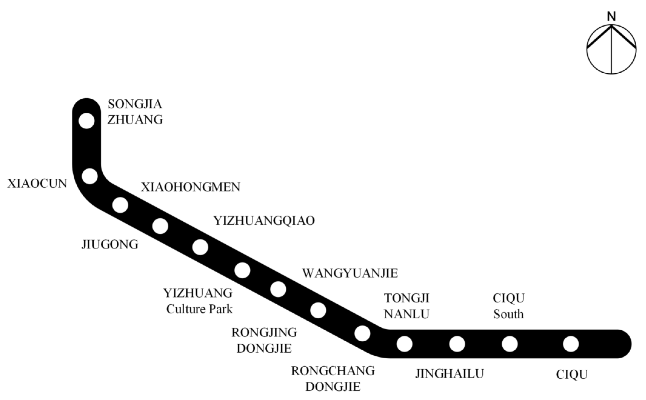
In this section, we applied our proposed model and ADP methods to the actual case of the Beijing Subway YIZHUANG Line, which consists of 13 stations, through three different experimental scenarios. During the morning peak hour, there is an apparent high passenger flow; thus, we only consider the up direction of the line from the Beijing Economic Technological Development Zone to the downtown. The time horizon is set from 7:30–8:30 when the passenger arrival rate is high and the headway is short. The first two scenarios were designed to verify the feasibility of the model, and the third one focused on the performance of the algorithm.

The map of the Beijing Subway YIZHUANG Line and its system parameters are shown in Figure 5 and Appendix A (

Table A1. Numerical characteristics of the YIZHUANG line.

Station	Index	${\mathit{s}}_{\mathit{i},\mathit{j}}^{min}$ (s)	${\mathit{D}}_{\mathit{i},\mathit{j}}$ (s)	${\mathit{s}}_{\mathit{i},\mathit{j}}^{max}$ (s)	Index	${\mathit{U}}_{\mathit{i},\mathit{j}}^{min}$ (s)	${\mathit{U}}_{\mathit{i},\mathit{j}}$ (s)	${\mathit{U}}_{\mathit{i},\mathit{j}}^{max}$ (s)
					-	-	-	-
CIQU South	1	10	25	60
					1	92	102	122
CIQU	2	10	25	60
					2	126	140	178
JINGHAILU	3	10	25	60
					3	135	150	180
TONGJINANLU	4	10	25	60
					4	148	164	197
RONGCHANGDONGJIE	5	10	25	60
					5	94	104	125
RONGJINGDONGJIE	6	10	25	60
					6	93	103	127
WANYUANJIE	7	10	25	60
					7	103	114	137
YIZHUANGCulture park	8	10	25	60
					8	81	90	108
YIZHUANGQIAO	9	10	25	60
					9	122	135	162
JIUGONG	10	10	25	60
					10	141	157	188
XIAOHONGMEN	11	10	25	60
					11	97	108	130
XIAOCUN	12	10	25	60
					12	171	190	228
SONGJIAZHUANG	13	10	25	60
					-	-	-	-

). Based on practice survey data and AFC records, the minimum and maximum running times are defined as 0.85-times and 1.2-times the scheduled running time. The upper and lower bounds of headway are 120 s and 400 s. The minimum dwell time for door opening and closing is 8 s.The capacity is 1480, and the overload ratio is 1.4. The number of doors is 24. The coefficients in the immediate cost are set as $0.6,0.2,0.2$. Besides, the algorithm parameters are all fixed in the experimental scenarios. Discount factor $\gamma$ is 0.9, and the maximum iteration N is 500 with a $1/N$ step size.

5.1. Scenario 1

To validate the feasibility and effectiveness of the model and algorithm presented in this paper, we first considered the situation where an equipment failure occurred in Section 2 for Train 2 and resulted in an arrival delay of 110 s. Owing to SONGJIAZHAUNG being a transfer station to the city, few passengers get off at the stations along the line. Therefore, in our experiments, the number of people alighting is proportional to the number of people in the vehicle, and the ratio is a small fixed value. Passenger arrival rate and alighting ratio are listed in

Table 2. Passenger arrival rate and alighting ratio.

Type	1	2	3	4	5	6	7	8	9	10	11	12	13
${\lambda }_{i,j}$	2.43	2.03	2.03	1.77	2.3	2.83	2.03	1.63	1.37	1.5	1.9	2.03	0
${\mu }_{i,j}$	0	0.01	0.01	0.01	0.01	0.01	0.01	0.01	0.01	0.01	0.01	0.01	1

.

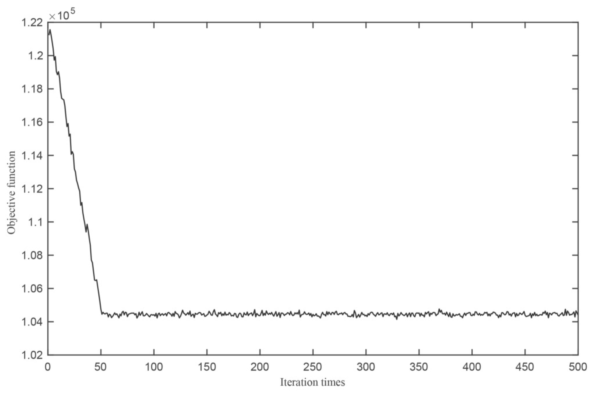
First, to demonstrate the validity of the ADP method we used in our proposed model, we compared the solving performance of policy iteration algorithms and the ADP method on the MATLAB platform. Due to the high effectiveness of the train operation adjustment problem, we concentrated more on the computational efficiency. It took 18 s to converge by the ADP method, as shown in Figure 6, while it took 123 s to get the optimal solution with a $2.3\times {10}^6$ total cost under the policy iteration strategy.

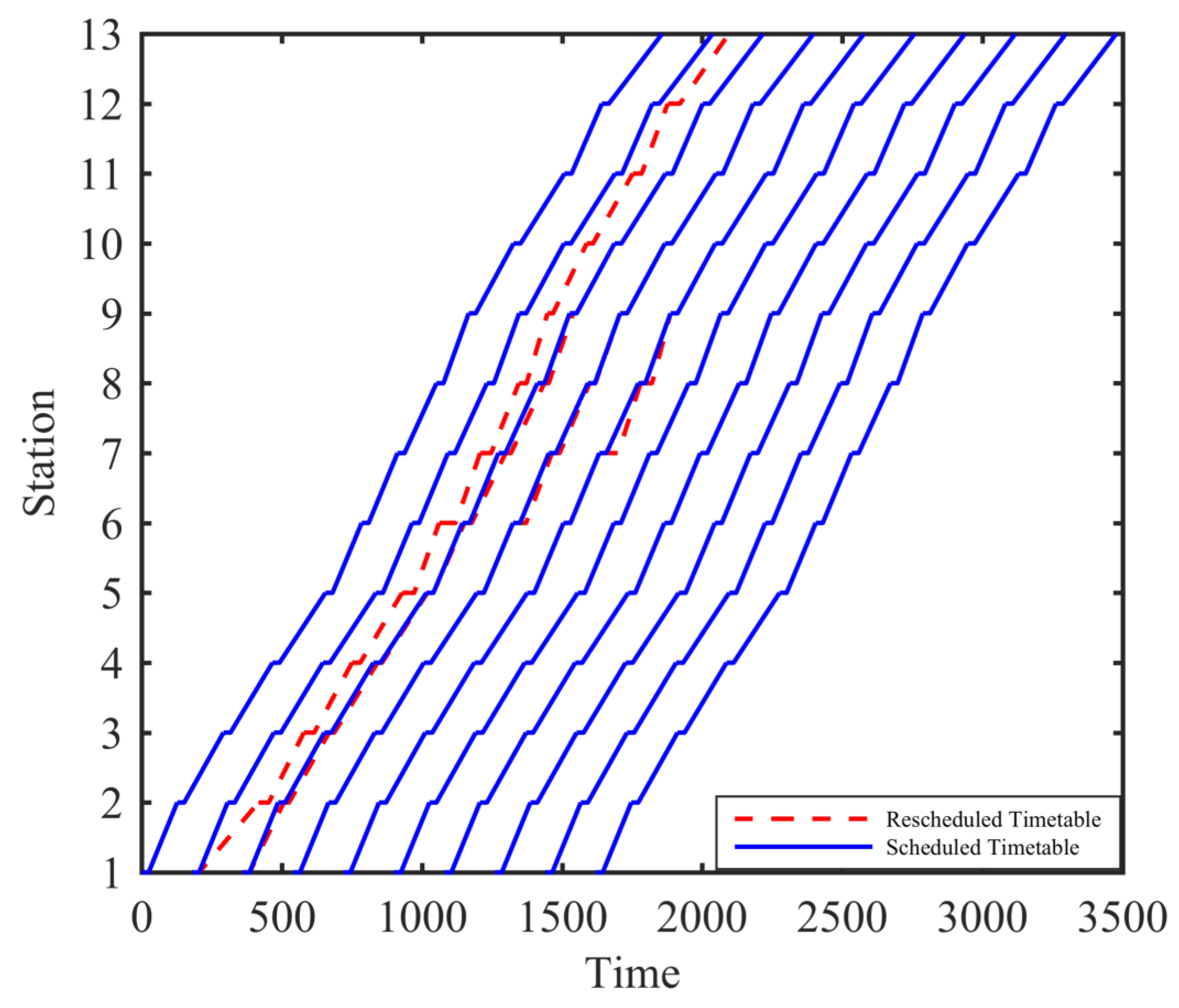
From

Table 3. Computation results of Scenario 1.

i	Station	1	2	3	4	5	6	7	8	9	1	11	12
$i=2$	$p_{i,j}$	0	6	5	5	5	6	6	5	4	3	2	2
	$u_{i,j}$	-	125	135	149	89	88	99	75	120	142	93	175
$i=3$	$p_{i,j}$	2	1	1	0	3	2	1	0	0	0	0	0
	$u_{i,j}$	121	143	154	162	111	121	119	87	135	168	113	188
$i=4$	$p_{i,j}$	0	0	0	0	0	0	0	0	0	0	0	0
	$u_{i,j}$	102	140	150	166	100	92	107	90	135	157	108	190

, we can conclude that the delay was effectively reduced through train regulation and passenger control to recover to the normal operation schedule as soon as possible. For the delayed Train 2 and the following affected train, some boarding passengers were restricted. The section running time was shortened, to avoid arriving too late at the latter station for Train 2, while being prolonged due to the headway constraint for Train 3. Furthermore, the number of passengers controlled reduced to zero gradually, and the running time returned to the scheduled value. Gradually, delay disappeared, and the train operation returned to normal. The comparison between the scheduled timetable and the rescheduled one is clear in Figure 7. Here, it should be clearly pointed out that although the two red lines of Train 2 and Train 3 are close to each other, they still meet the minimum headway constraint.

5.2. Scenario 2

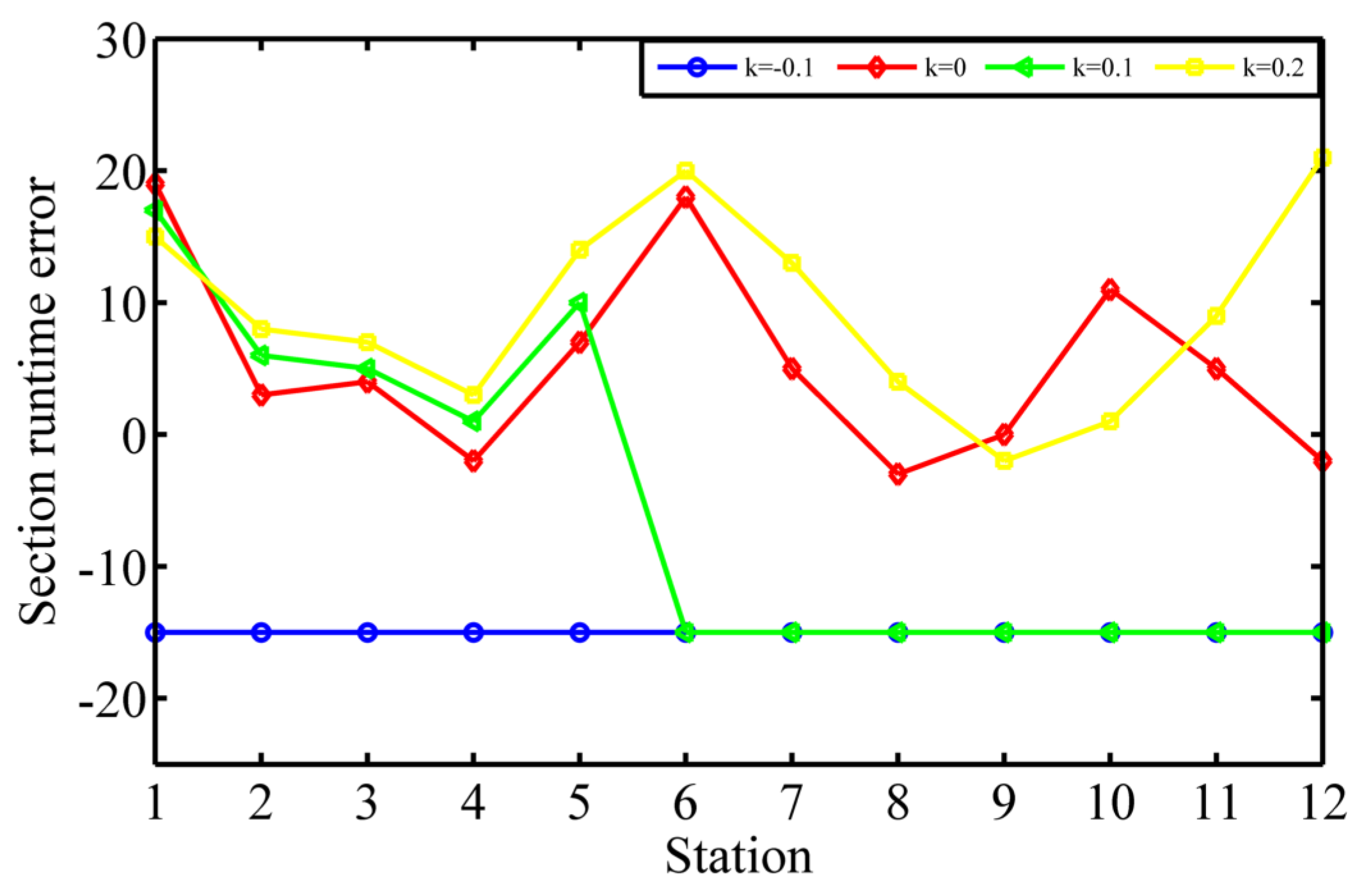
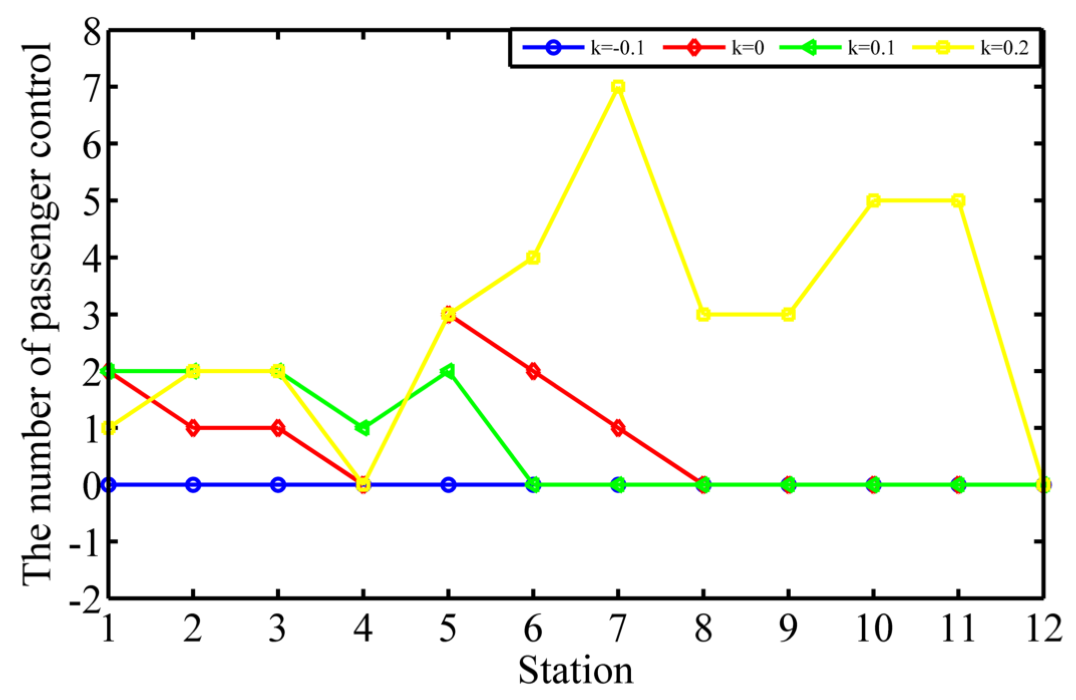
In the former scenario experiment, the delay was caused by systemic disorder, and we assumed the passenger arrival rate was constant. However, in the actual operation, there is also another disturbance that is caused by a sudden increase in passenger flow sometimes. Therefore, we designed the second scenario experiment to analyze the sensitivity to passenger flow of the proposed model and algorithm in this paper. All rates in this case fluctuated with a small increment k. Due to the limitation of length for the manuscript, we just chose the solution results of the first followed train affected by the delayed train and used Figure 8 and Figure 9 to reveal its features of change.

From the two figures, something interesting can be concluded. First, when the rate was relatively small, the number of passengers controlled was zero, which is consistent with the actual situation. That is because the scheduled dwell time was sufficient enough, in addition to the time for passenger alighting and boarding; there was no need to sacrifice the benefit to passenger, and it was easy to recover to the normal operation only by regulating the section running time. Moreover, with the increase of arriving passengers, exclusively changing the running time did not work, and the passenger control strategy was supposed to be adopted, which makes sense. The higher the rate, the greater the degree of delay that may result, and more passengers should be controlled. By comparison, there is something else notable: the change of the running time was not monotonous. Although our goal was to dissipate the delay, the section running time was not reduced all the time due to the headway constraint.

These results also prove that our model does consider both dynamic passenger flow and operating characteristics, and it can reflect the impact of passenger flow on operations. Such adjustment measures are also applicable to sudden large passenger flow situations. Passenger control can flexibly regulate dwell time, meeting the demand of reasonable deployment for transportation resources well.

5.3. Scenario 3

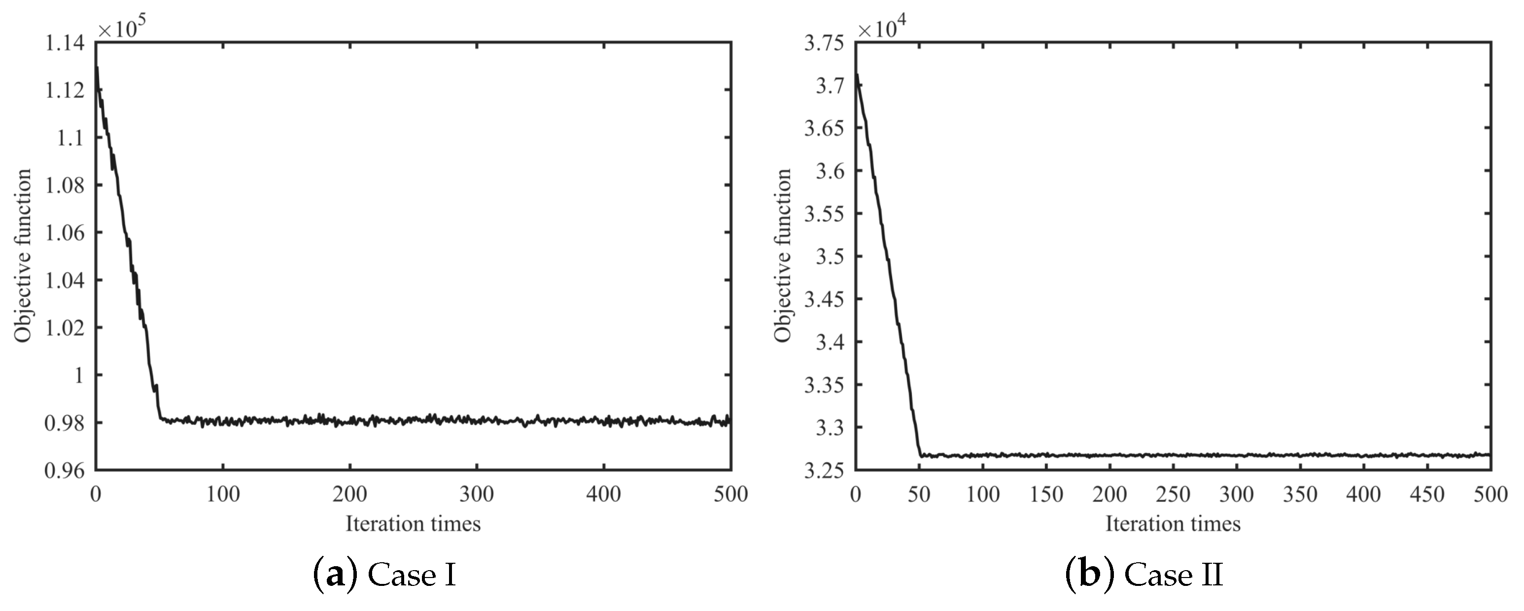
In this scenario, we further investigated the model application in situations where delay occurs at different station and for different train. By comparison, the extensive applicability was verified. The different initial delays are shown in

Table 4. Setting of different delay circumstances.

Case	Arrival Delay (s)
Train 2 at Station 2	70
Train 3 at Station 3	110

. Other parameters were identical to scenario 1.

Convergence results are explicitly shown in Figure 10. In each case, objective functions converged at about the 50th iteration. Actually, this iterative update method involves the idea of machine learning. Although we did not have the real value, we could substitute it with other targets. The historical results of each cycle were used as sample data, by which exploration and exploitation were used to work out the optimal policy.

As we discussed before, the regulation models in other literature works have limitations to consider the indices of train running simply. However, we found that with the contradiction between demand and supply getting more serious, the impact of passenger flow fluctuations on operations can become more apparent, and the passenger control variable and running time variable were sensitive to environmental changes. Through the above three experimental scenarios, we have proven the necessity of passenger control and verified the effectiveness of our model in different situations.

6. Conclusions

This paper studies the train adjustment problem under dynamic passenger flow and establishes a model combined train regulation with passenger control. First, we selected the number of passengers for flow control and the section running time as two decision variables and then divided the complex adjustment process into multiple decision-making stages. Compared with other works, our model links the train operation adjustment with the passenger flow control based on the Markov decision process to describe the interaction process visually, and we also took both operation costs and passenger loss into account. As for the algorithm, the ADP method used in this paper significantly improved the computational efficiency, satisfying the real-time performance of train operation regulation in different experimental scenarios. We approximated the value function with the basic function formulated with feature variables, which solved the dimension problem. Besides, the results showed that the passenger control measure can be suitable for uncrowded and overcrowded situations. In future work, we will pay more attention to the algorithm performance of different parameter values. It is an interesting work to study the travel behavior of passengers under the passenger control situation.

References

- Cacchiani, V.; Huisman, D.; Kidd, M.; Kroon, L.; Toth, P.; Veelenturf, L.; Wagenaar, J. An overview of recovery models and algorithms for real-time railway rescheduling. Transp. Res. Part B Methodol. 2014, 63, 15–37. [Google Scholar] [CrossRef]
- Goodman, C.; Murata, S. Metro traffic regulation from the passenger perspective. Proc. Inst. Mech. Eng. Part F J. Rail Rapid Transit 2001, 215, 137–147. [Google Scholar] [CrossRef]
- D’riano, A.; Pacciarelli, D.; Pranzo, M. A branch and bound algorithm for scheduling trains in a railway network. Eur. J. Oper. Res. 2007, 183, 643–657. [Google Scholar] [CrossRef]
- Acuna-Agost, R.; Michelon, P.; Feillet, D.; Gueye, S. A MIP-based local search method for the railway rescheduling problem. Networks 2015, 57, 69–86. [Google Scholar] [CrossRef]
- Sheu, J.W.; Lin, W.S. Adaptive Optimal Control for Designing Automatic Train Regulation for Metro Line. IEEE Trans. Control Syst. Technol. 2012, 20, 1319–1327. [Google Scholar] [CrossRef]
- Yin, J.; Tao, T.; Yang, L.; Gao, Z.; Ran, B. Energy-efficient metro train rescheduling with uncertain time-variant passenger demands: An approximate dynamic programming approach. Transp. Res. Part B Methodol. 2016, 91, 178–210. [Google Scholar] [CrossRef]
- Xiang, L.; Hong, K.L. Energy minimization in dynamic train scheduling and control for metro rail operations. Transp. Res. Part B 2014, 70, 269–284. [Google Scholar]
- Van Breusegem, V.; Campion, G.; Bastin, G. Traffic modeling and state feedback control for metro lines. IEEE Trans. Autom. Control 1991, 36, 770–784. [Google Scholar] [CrossRef] [Green Version]
- Dorfman, M.J.; Medanic, J. Scheduling trains on a railway network using a discrete event model of railway traffic. Transp. Res. Part B 2004, 38, 81–98. [Google Scholar] [CrossRef]
- Xu, X.; Li, K.; Yang, L. Rescheduling subway trains by a discrete event model considering service balance performance. Appl. Math. Model. 2016, 40, 1446–1466. [Google Scholar] [CrossRef]
- Wang, P.; Lei, M.; Goverde, R.M.P.; Wang, Q. Rescheduling Trains Using Petri Nets and Heuristic Search. IEEE Trans. Intell. Transp. Syst. 2016, 17, 726–735. [Google Scholar] [CrossRef]
- Yin, J.; Chen, D.; Yang, L.; Tao, T.; Ran, B. Efficient Real-Time Train Operation Algorithms With Uncertain Passenger Demands. IEEE Trans. Intell. Transp. Syst. 2016, 17, 2600–2612. [Google Scholar] [CrossRef]
- Chang, S.C.; Chung, Y.C. From timetabling to train regulation—New train operation model. Inf. Softw. Technol. 2005, 47, 575–585. [Google Scholar] [CrossRef]
- Krasemann, J.T. Design of an effective algorithm for fast response to the re-scheduling of railway traffic during disturbances. Transp. Res. Part C Emerg. Technol. 2012, 20, 62–78. [Google Scholar] [CrossRef]
- Albrecht, A.R.; Panton, D.M.; Lee, D.H. Rescheduling rail networks with maintenance disruptions using Problem Space Search. Comput. Oper. Res. 2013, 40, 703–712. [Google Scholar] [CrossRef]
- Fischetti, M.; Monaci, M. Using a general-purpose Mixed-Integer Linear Programming solver for the practical solution of real-time train rescheduling. Eur. J. Oper. Res. 2017, 263, 258–264. [Google Scholar] [CrossRef]
- Li, S.; Dessouky, M.M.; Yang, L.; Gao, Z. Joint optimal train regulation and passenger flow control strategy for high-frequency metro lines. Transp. Res. Part B Methodol. 2017, 99, 113–137. [Google Scholar] [CrossRef]
- Chang, H.S.; Lee, H.G.; Fu, M.C.; Marcus, S.I. Evolutionary policy iteration for solving Markov decision processes. IEEE Trans. Autom. Control 2002, 50, 1804–1808. [Google Scholar] [CrossRef]
- Powell, W.B. Approximate Dynamic Programming: Solving the Curses of Dimensionality; John Wiley & Sons, Inc.: Hoboken, NJ, USA, 29 March 2007. [Google Scholar]
- Feng, L.; Wu, Q.; Wang, Y.; Ying, Q. An approximate dynamic programming approach for network capacity control problem with origin-destination demands. Int. J. Model. Identif. Control 2011, 13, 195–201. [Google Scholar]
- Fang, J.; Zhao, L.; Fransoo, J.C.; Van Woensel, T. Sourcing strategies in supply risk management: An approximate dynamic programming approach. Comput. Oper. Res. 2013, 40, 1371–1382. [Google Scholar] [CrossRef]
- Meissner, J.; Senicheva, O.V. Approximate dynamic programming for lateral transshipment problems in multi-location inventory systems. Eur. J. Oper. Res. 2018, 265, 49–64. [Google Scholar] [CrossRef]
- Goverde, R.M.P. A delay propagation algorithm for large-scale railway traffic networks. Transp. Res. Part C Emerg. Technol. 2010, 18, 269–28711. [Google Scholar] [CrossRef]
- Yuan, J. Stochastic Modelling of Train Delays and Delay Propagation in Stations; Eburon Academic Publisher: Delft, The Netherlands, 2006. [Google Scholar]
- Cucala, A.P.; Fernández, A.; Sicre, C.; Domínguez, M. Fuzzy optimal schedule of high speed train operation to minimize energy consumption with uncertain delays and driver’s behavioral response. Eng. Appl. Artif. Intell. 2012, 25, 1548–1557. [Google Scholar] [CrossRef]
- Lin, T.m.; Wilson, N.H. Dwell time relationships for light rail systems. Transp. Res. Rec. 1992, 1361, 287–295. [Google Scholar]
- Lamorgese, L.; Mannino, C. An exact decomposition approach for the real-time train dispatching problem. Oper. Res. 2015, 63, 48–64. [Google Scholar] [CrossRef]
- Zhang, B.C.; Yi, L. Research on Dwelling Time Modeling of Urban Rail Transit. Traffic Transp. 2011, 27, 48–52. [Google Scholar]
- Sutton, R.; Barto, A. Reinforcement Learning: An Introduction, 2nd ed.; MIT Press: Cambridge, MA, USA, 1998. [Google Scholar]
Figure 1.
Train operation on the single metro line.
Figure 2.
The illustration of passengers accumulating.
Figure 3.
The illustration of train regulation combined with passenger control.
Figure 4.
Markov decision process.
Figure 5.
Beijing Subway YIZHUANGXIAN Line.
Figure 6.
Convergence of the objective function.
Figure 7.
Train distance-time diagram.
Figure 8.
Section running time error.
Figure 9.
The number of passengers controlled.
Figure 10.
Convergence of the two cases.