Multi-Agent Reinforcement Learning Using Linear Fuzzy Model Applied to Cooperative Mobile Robots


1
Department of industrial engineering and manufacturing, Autonomous University of Ciudad Juarez, Ciudad Juarez 32310, Mexico
2
Faculty of mechanical and electrical engineering, Autonomous University of Coahuila, Torreon 27276, Mexico
*
Author to whom correspondence should be addressed.
Symmetry 2018, 10(10), 461; https://doi.org/10.3390/sym10100461
Submission received: 5 September 2018
/
Revised: 24 September 2018
/
Accepted: 30 September 2018
/
Published: 3 October 2018
(This article belongs to the Special Issue Symmetry in Complex Systems)
Abstract
:A multi-agent system (MAS) is suitable for addressing tasks in a variety of domains without any programmed behaviors, which makes it ideal for the problems associated with the mobile robots. Reinforcement learning (RL) is a successful approach used in the MASs to acquire new behaviors; most of these select exact Q-values in small discrete state space and action space. This article presents a joint Q-function linearly fuzzified for a MAS’ continuous state space, which overcomes the dimensionality problem. Also, this article gives a proof for the convergence and existence of the solution proposed by the algorithm presented. This article also discusses the numerical simulations and experimental results that were carried out to validate the proposed algorithm.
1. Introduction
Multi-agent systems (MASs) are finding application in a variety of fields where pre-programmed behaviors are not a suitable way to tackle the problems that arise. These fields include robotics, distributed control, resource management, collaborative decision making, data mining [1]. A MAS includes several intelligent agents in an environment, where each one has its independent behavior and should coordinate with the others [2].
MASs could emerge as an alternative way to analyze and represent the systems with centralized control, where several intelligent agents perceive and modify an environment through sensors and actuators respectively. At the same time, these agents can also learn new behaviors to adapt themselves to the new tasks and the goals in an environment [3].
One of the fields where multi-agent systems have emerged are mobile robots, most approaches are based on low level control systems, in [4] a visibility binary tree algorithm is used to generate the mobile robot trajectories. This type of approach is based on the complete knowledge of the dynamics of the robotic system. In this article, we offer a proposal based on reinforcement learning, which will result in high-level control actions.
Reinforcement learning (RL) is one of the most popular methods for learning in a MAS. The objective of a Multi-agent reinforcement learning (MARL) is to maximize a numerical reward; so that, the agents can interact with the environment and modify it [5]. At each learning step, these agents choose an action, which drives the environment to a new state [6]. The Reward function assesses the grade of this state transition [7]. In the RL the agents are not told which tasks should be executed instead they must explore which actions have the best reward. Hence, the RL feedback is less informative than a supervised learning method [8].
MASs are affected by the curse of dimensionality, which is a term given to suggest that the computational and memory requirements increase as the number of states or agents increase in an environment. Most approaches require an exact representation of the state-action pair values in the form of lookup tables, making the solution intractable, hence the application of these methods is reduced to small or discrete tasks [9]. In the real-life applications, the state variables can be a selected from of a large number of possible values or even from the continuous values; so, the problem is manageable if value functions are approximated [10].
Some MARL algorithms have been proposed to deal with this problem using neural networks by making generalizations from a Q-table [11], applying function approximation for discrete and large state-action space [12], applying vector quantization for continuous state and actions [13], using experience replay for MAS [14], using Q-learning and normalized Gaussian network as approximators [15], predictions in systems with heterogeneous agents [16]. In [17] a couple of neural networks is used to represent the value function and the controller, however, the proposed strategy is based on a sufficient exploration, which is a function of the size of the training data of the neural networks. Inverse neural networks have also been proposed to approximate the actions policy, which uses an initial policy of actions to be refined through reinforcement learning [18].
This article presents an approach for MARL in a cooperative problem. It is a modified version of the Q-learning algorithm proposed in [19] which uses a linear fuzzy approximator of the joint Q-function for a continuous state space. An implicit form of coordination is implemented to solve the coordination problem. An experiment is conducted on two robots performing the task of solving a coordination problem to verify the proposed algorithm. In addition to that, two theorems are presented to ensure the convergence of the proposed algorithm.
2. MARL with Linear Fuzzy Parameterization
2.1. Single Agent Case
In a reinforcement learning (RL) for a single agent case, let us define: as the current state of the environment at the learning step k, and as the action taken by the agent in .
The reward or the numerical feedback, , reflects how good was the previous action, , in the state . The single agent RL problem is a Markov decision process (MDP). MDP for a deterministic case is:
where X is the state space, U is the actions space, f is the state transition function which can be known or unknown, and is the reward scalar function.
The action policy is used to describe the agent’s behavior, which specifies the way in which the agent chooses the action from a state. If the action policy, , does not change over time it is considered stationary [20].
The final goal is to find an action policy h such that the long-term return R is maximized:
where is the discount factor. The policy, h, is obtained from the state-action value function, called Q-function.
The Q-function
gives a expected return from the policy, h,
The optimal Q-function is defined as:
Once is available, the optimal action policy is obtained by:
2.2. Multi Agent System Case
In a Multi-agent case, there is some number of heterogeneous agents with their own set of actions and tasks in an environment. A stochastic game model describes this behavior in which the action performed at any state is a combination of the actions by each agent [21].
The deterministic stochastic game’s model is a tuple , where n is the number of the agents in the environment, X is the state of the environment, are the sets of actions available to each agent and the joint action set . The reward functions , and the state transition function is .
The joint action , , taken in the state , changes the state to . A numerical value for the reward is calculated as for each joint action . The actions are taken according to each agent’s own policy , where all of them form the joint policy . Similar to a single agent case, the state space and actions space can be continuous or discrete.
The long term reward R depends on the joint policy due to the numerical feedback r of each agent depends on the joint action . Thereby the Q-function of each agent relies on the joint action and the joint policy, , with .
Each agent could have its own goals, however, in this article the agents seek a common goal, i.e., the task is fully cooperative. In this way the numerical feedback or reward for any state is the same for all agents , therefore the reward scalar functions and returns are the same for all the agents, . Hence the agents have the same goal which is maximize the common long term performance (or return).
Determining an optimal joint policy in Multi-agent systems is the equilibrium selection problem [22]. Although establishing an equilibrium is a difficult problem, the structure of the cooperative settings make this problem manageable. Assuming that the agents know the structure of the game in the form of the transition function f and the reward function makes the searching of the equilibrium point more tractable.
In a fully cooperative stochastic game, if the transition function f and the reward function for each agent is known, the objective can be accomplished by learning the optimal joint-action values through Bellman optimal equation: and then using a greedy policy [23]. Once is available, a policy h is:
When several joint actions are optimal the agents could choose different actions and degrade the performance of the search for a common goal. This problem can be solved by: the coordination free methods assume that the optimal join action are unique across learning a common Q-function [24], the coordination-based methods use the coordination graphs through a decomposition of the global Q-function in local Q-functions [25], or the implicit coordination methods assume the agents learn to choose one joint action by chance and then discard the others [26].
2.3. Mapping the Joint Q-Function for MAS
In a deterministic case, the Q-function, Q, is
with an arbitrary initial value for Q. The iterations (8) attracts the Q to a unique fixed point at [27]
In [28] is shown that the mapping is a contraction with factor . For any pair of Q-function and
and then H has a unique fixed point. is a fixed point of H: , and the iteration converges to as An optimal policy can be calculated from using (8). To perform the former iteration, we need a model of the task in the form of the transition function f and reward function
This kind of method, based on the Bellman optimality equation, need saving and updating the Q-values for each state-joint action stage. In this way, only tasks with finite discrete set of state and actions are generally treated. The dimensionality problems occur by the growth of the number of agents involved in the task [29], thus this generates an increment on the computational complexity [30].
In the case where the state space or actions space are continuous or even discrete with a great number of variables, the Q-functions must be depicted in an approximated form [31]. Because an exact representation of the Q-function could be impractical or intractable, therefore, we propose an approximate linear fuzzy representation of the joint Q-function through a vector .
2.4. Linear Fuzzy Parameterization of the Joint Q-Function
In general, if there is no prior awareness about the Q-function, the only form to have an exact representation is saving distinct Q-values for each state-action couple. If the state space is continuous, the exact representation of the Q-function would need take an infinite number of state-action values. For this reason, the only practical way to overcome this situation is using an approximate representation of the joint Q-function.
In this section, we present a parameterized version of the Q-function through a linear fuzzy approximator which consist in a vector , this vector relies in a fuzzy partition of the continuous state space. The principal advantage of this proposal is that we only need to save the state-action pair Q-value of the center of every membership function.
There are N fuzzy sets, which are depicted by a membership function:
where describe the degree of membership of the state x to the fuzzy set this membership functions can be looked as basis functions or features [32]. The number of membership functions increase with the size of the state space, the number of the agents and with the degree of resolution sought for the vector
Triangular shapes of fuzzy partitions are used in this paper since they have their maximum value in a single point, namely, for every d exist a unique (the core of the membership function) such that Since all the others membership functions take zero values in , for ∀ , we assume that , which mean that the membership functions are normal. Another kind of Membership Functions shape could diverge when they have too big values in [33].
We have a number N of triangular membership functions for each state variable , with A pyramid shape E dimensional of membership functions will be the consequence of the product of each single dimensional membership function in the fuzzy partition of the state space.
We assume that the action space is discrete for all the agents and they have the same number of actions available:
The parameter vector is composed by elements to be stored, the membership function-action pair for each agent correspond an element of the parameter vector . The approximator’s elements are organized in a preliminary way using n different matrices with size , filling the first M columns with the N elements available. The elements of the n matrix are allocated in a vector arrangement column by column for the first agent, then follow with the next agent’s columns until completing n agents.
Denoting the scalar indexes of by:
where means the number of the analyzed agent, is the number of fuzzy partitions for each state variable , with and In this way we denote the indexes of the parameter approximator by , which means the approximate Q-value for the d membership function, performing the action j available for the agent
The state x is taken as input by the fuzzy rule base and produces M outputs for each agent, which are the corresponding Q-values to each action for every agent the function’s outputs are the elements of The fuzzy rule base proposed can be considered as a zero order Takagi-Sugeno rule base [34]:
The approximate Q-value can be calculated by:
The expression (13) is a linear parameterized approximation, the Q-values of a specified state-action couple is estimated through a weighted sum, where the weights are generated by the membership functions [35]. This approximator can be denoted by an approximator mapping
where is the parameter space, the parameter represents the approximation of the Q-function:
Thus we do not need to store a great amount of Q-values for every pair Only z parameters in are needed. The mapping approximator F only represents a subset of [36].
From the point of view of reinforcement learning, a linear parameterized approximation of F are preferred since they make more suitable to analyze the theoretical aspect. This is the reason for our choosing of using a linear parameterized approximation , in this way, the normalized membership functions can be considered as basis functions [37].
The Expression (15) provides a which is an approximate Q-function, in place of the exact Q-function Q, so the approximate is supplied to the mapping H:
Most of the time the Q-function is not able to be stored in a explicit way [38], as alternative, it has to be represented in an approximate form using a projection mapping
which makes certain that is as near as possible of [39], in the sense of least square regression:
where a set of state-joint actions samples are used. Because of the use of triangular membership function shapes, and the linear parameterized approximation mapping F, (18) is a convex quadratic optimization problem where samples are used [40], so the expression (18) is reduced to a designation in the form:
Recapitulating, the approximate linear fuzzy representation of the joint Q-function begins with an arbitrary value of the vector parameter vector and actualizes it in each iteration using the mapping:
and stops when a parameter threshold is greater than the difference between 2 consecutive parameters vector
A greedy policy can be obtained to control the system from (which is the parameter vector derived when ), for whichever state, the actions are calculated by interpolation between the best local actions for each agent for every membership function center :
To implement the update (20), we propose a procedural using a modified version of the Q-learning algorithm [19], where the linear parameterization is added, in this way the algorithm can be extended to Multi-agent problems with continuous state space but with discrete action space. The algorithm starts with an arbitrary (it can be ) until a threshold is reached after several iterations.
2.5. Reinforcement Learning Algorithm for Continuous State Space
The linear fuzzy approximation depicted by (20) can be described by the following algorithm, where is used a modified version of Q-learning algorithm. To set a correspondence among the algorithm and the expression (20), the right hand of step 2 can be seen as (16) and then using the expression (17). Here the dynamics f, the reward function and the discount factor are known in the form of a batch sample data.
- Let , setwhere is the probability of choose a greedy action in the state x, and is the probability of choose a random joint-action in
- Repeat in each iteration k
- For state we select a joint action with a suitable exploration. At each step a random action with probability is used.
- Applying the linear fuzzy parameterization with membership functions and discrete actions , the threshold
- Until:
- Output:
A greedy policy is obtained to control the system by:
where is the optimal action for the center for the agent i.
Theorem 1.
The algorithm with linear fuzzy parameterization (20) converges to a fixed vector .
Proof of Theorem 1.
Since the mapping given by
the convergence of the algorithm is guaranteed through ensuring that the compound mapping is a contraction in the infinite norm. [28] shows that the mapping H is a contraction, so it remains to demonstrate that F and P are not expansions. The mapping given by F is a weighted linear combination of membership functions
where the last step is true because the sum of the standard functions is and the product generated by each agent also is So it shows that the mapping F is a non-expansion. Since the mapping P is
and the samples are centers of the membership functions so the mapping P is a non-expansion [33]. Since H mapping is a contraction with , so is also a contraction by the factor
where has a fixed vector and the algorithm above converges to this fixed point as . ☐
Theorem 2.
For any choice of and any initial threshold value parameter vector , the algorithm with linear fuzzy parameterization is completed in a finite time.
Proof of Theorem 2.
As shown in Theorem 1, the mapping is a contraction with and a fixed vector
So, if for induction for . According to Banach fixed point, is bounded. Since the vector where the iteration starts is bounded, then is also bounded. Let which is bounded and for , applying the triangle inequality:
If
Applying log base on both side of the above expression
with which is bounded and implies that k is finite. So the algorithm is arrived in the most k iterations. ☐
3. Results
3.1. Simulation of a Cooperative Task with Mobile Robots
We perform a simulation where the linear fuzzy parameterization is applied to a two-dimensional Multi-agent cooperative problem with continuous states and discrete actions. The two agents with mass m have to be directed in a flat surface, such that they reach the origin at the same time with minimum time elapsed. The information available to the agents consists of the reward function, the transition function of states and joint actions.
In the simulation environment, the state has the coordinates in two dimensions of each agent , and their velocities in two dimensions , for : . The continuous state space model of the simulated system is:
where for is the function friction which depends of the position of each agent, the control signal is which is a force and for is the mass of each robot.
The system is discretized with a step of and the expression that describes the dynamics of the system are integrated between the sampling time. In the task, we select the start points randomly and carry out 50 training iteration, in the case of reaching 50 iterations without accomplishing the final goal, the experiment is restarted.
The magnitude of the state and action variables are bounded. To make more tractable the problem, and meters, and , also the force is bounded for , the friction coefficient is taken constant with , the mass of the agent is taken equal for both kg.
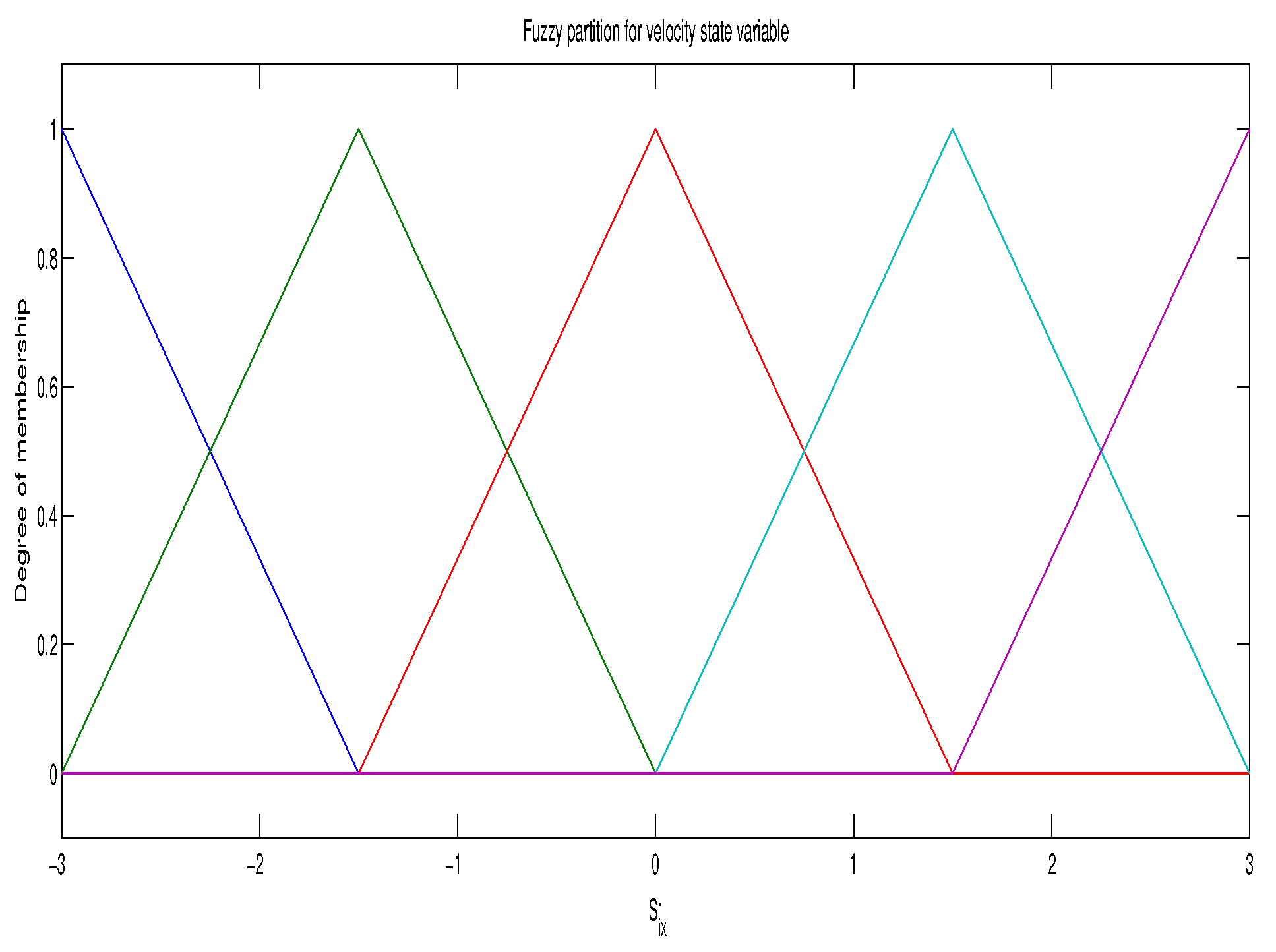
The actions control for each agent are discrete with 25 elements 0 0 for , they correspond to force in diagonal, left, right, up, down and no force applied. The membership functions used for the position state and velocity state have triangular shape, where the core of each membership function is . The cores of the membership function for the location domain s is centered at and the cores of the membership function for the velocity domain are: each one for every agent, this is shown in Figure 1. In this way 50625 pairs are storage for each agent in the vector parameter , this amount increases with the number of membership functions. An example of fuzzy triangular partition is showed in Figure 1.
The partition of the state space x is determined by the product of the individual membership function for each agent i
The final objective of arriving at the same is shown by a common reward function :
As regards the coordination problem, the agents accomplish an implicit coordination, where they learn to prefer one solution about equally good solutions by chance and then overlook the other options [41].
After the algorithm is performed and is obtained, a policy can be derived by interpolation between the best local action for each agent:
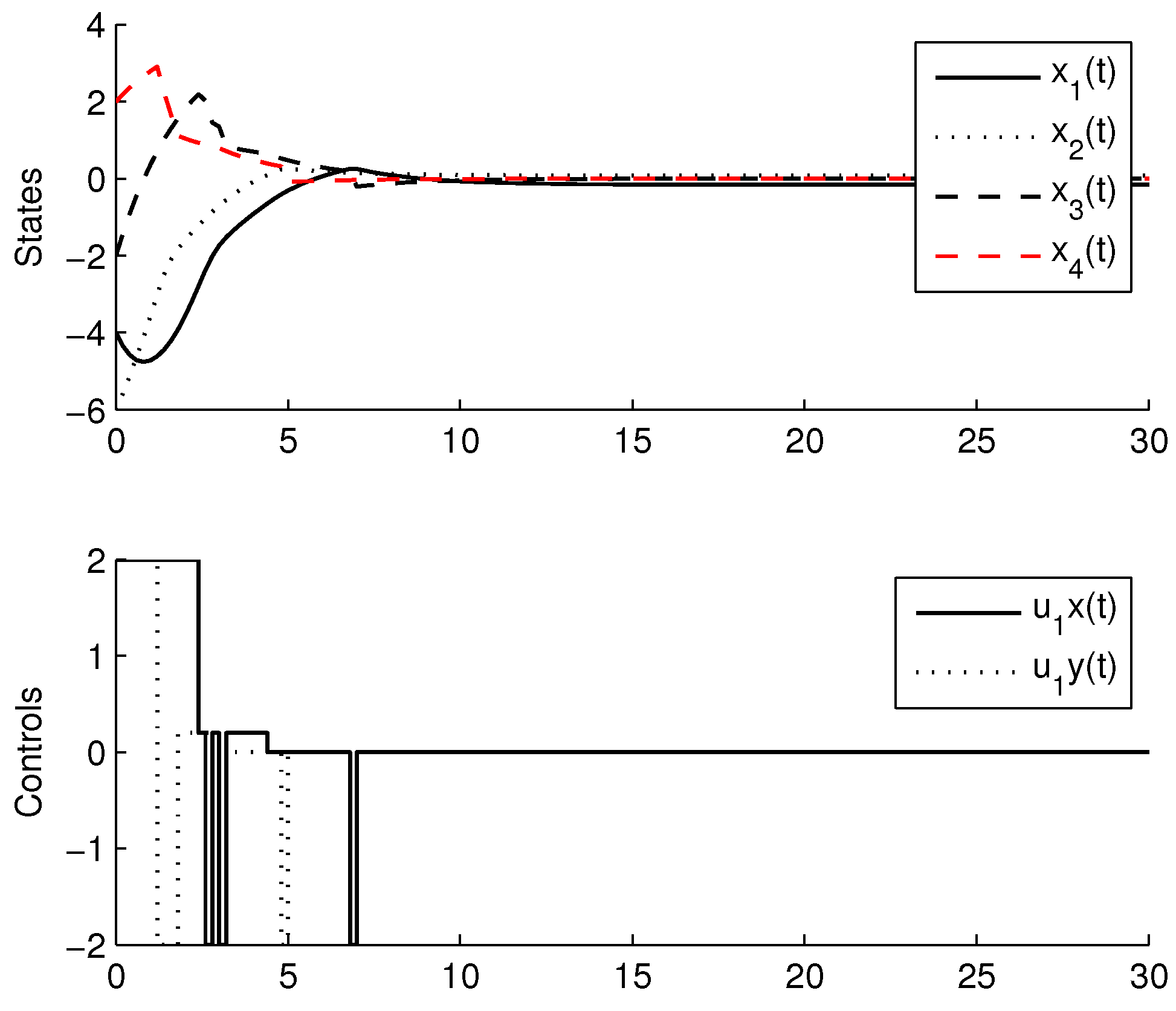
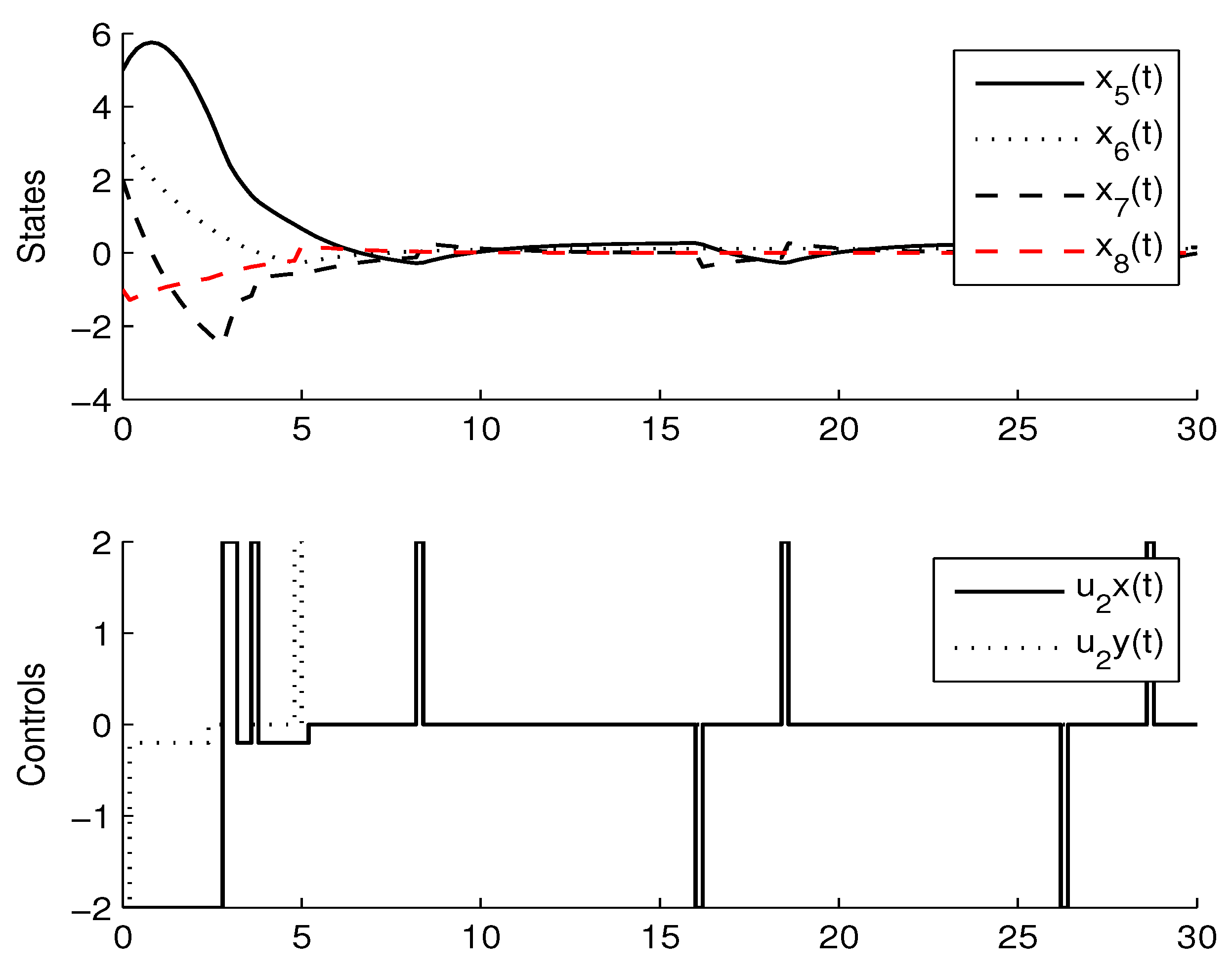
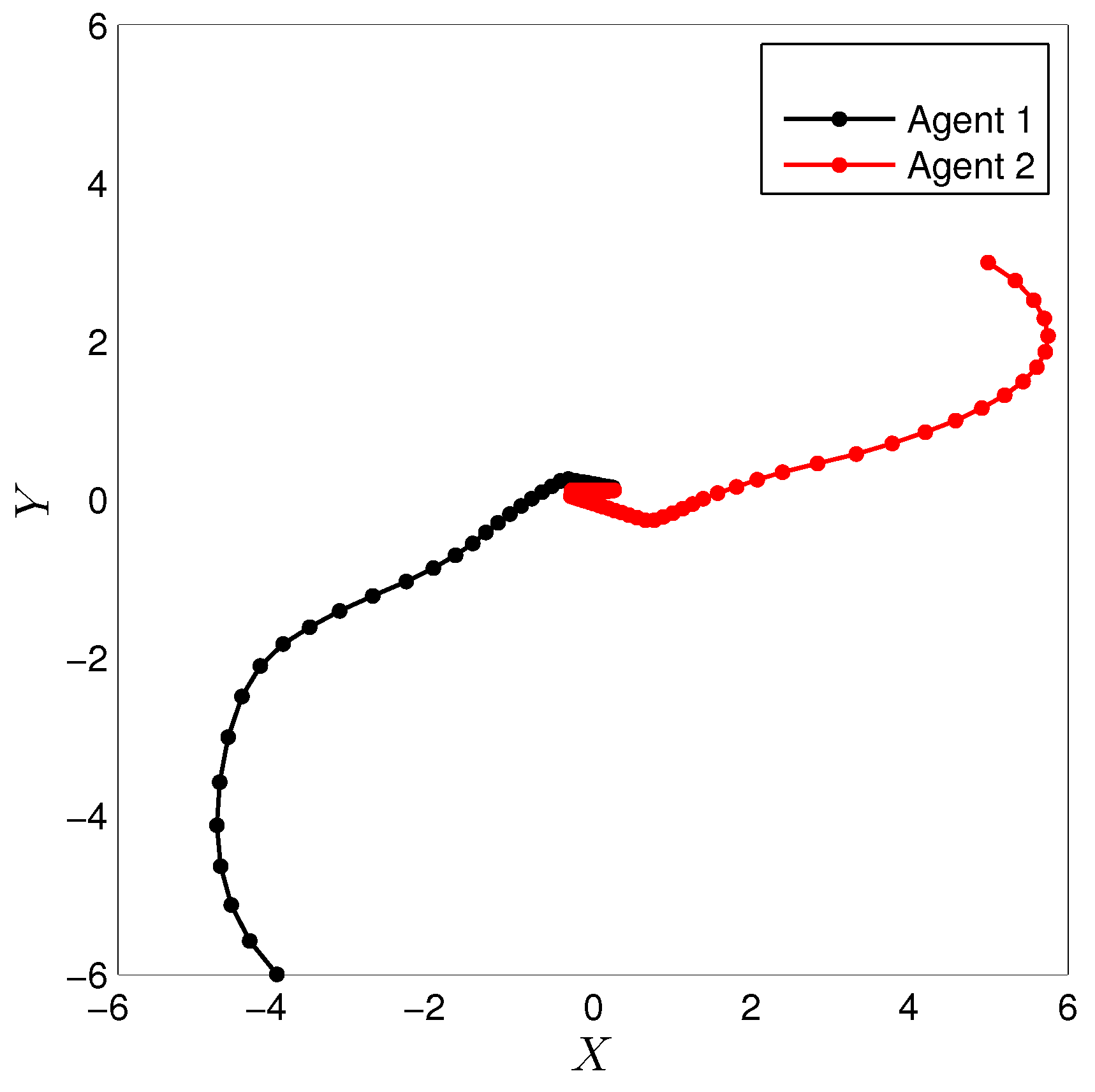
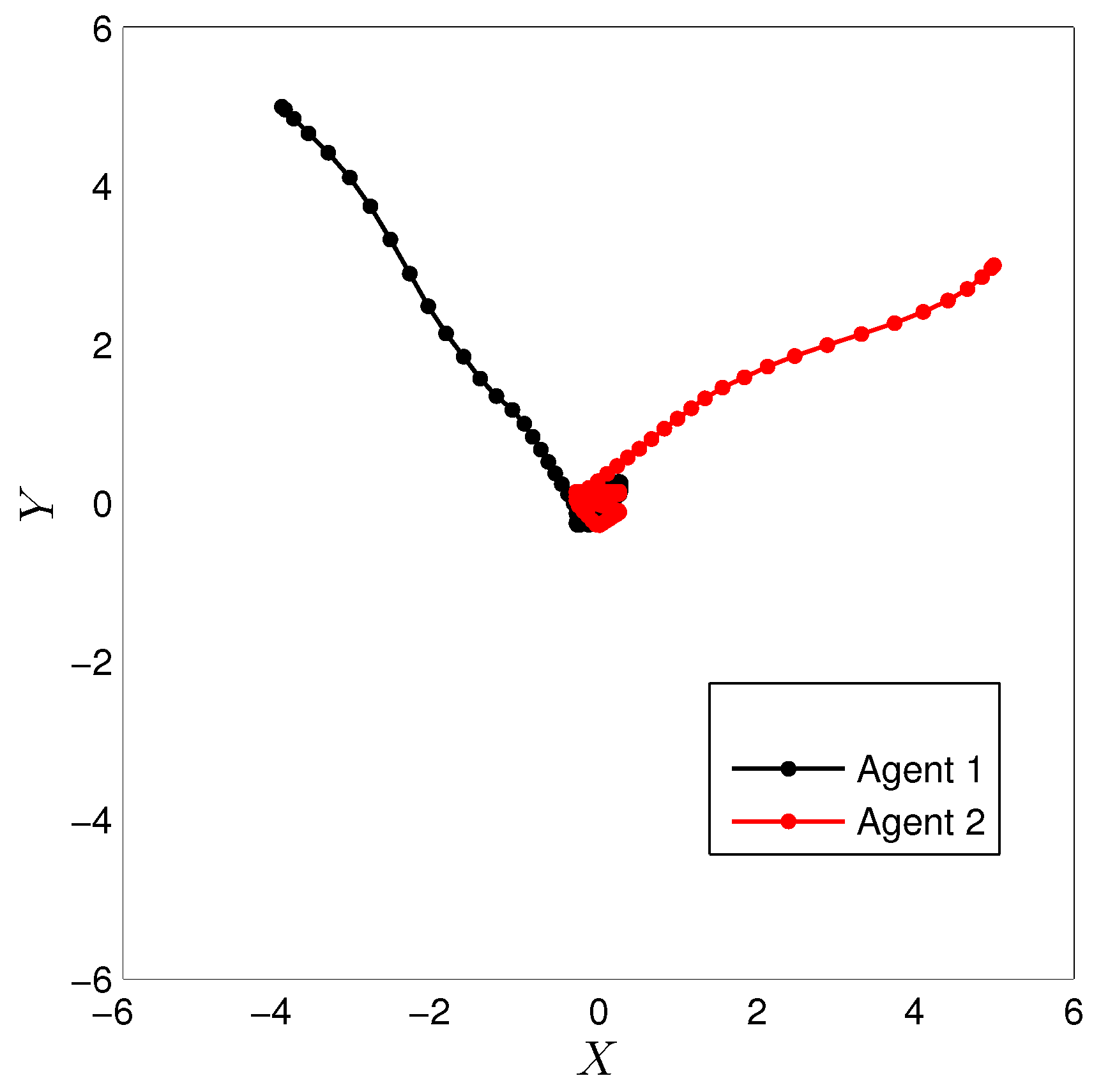
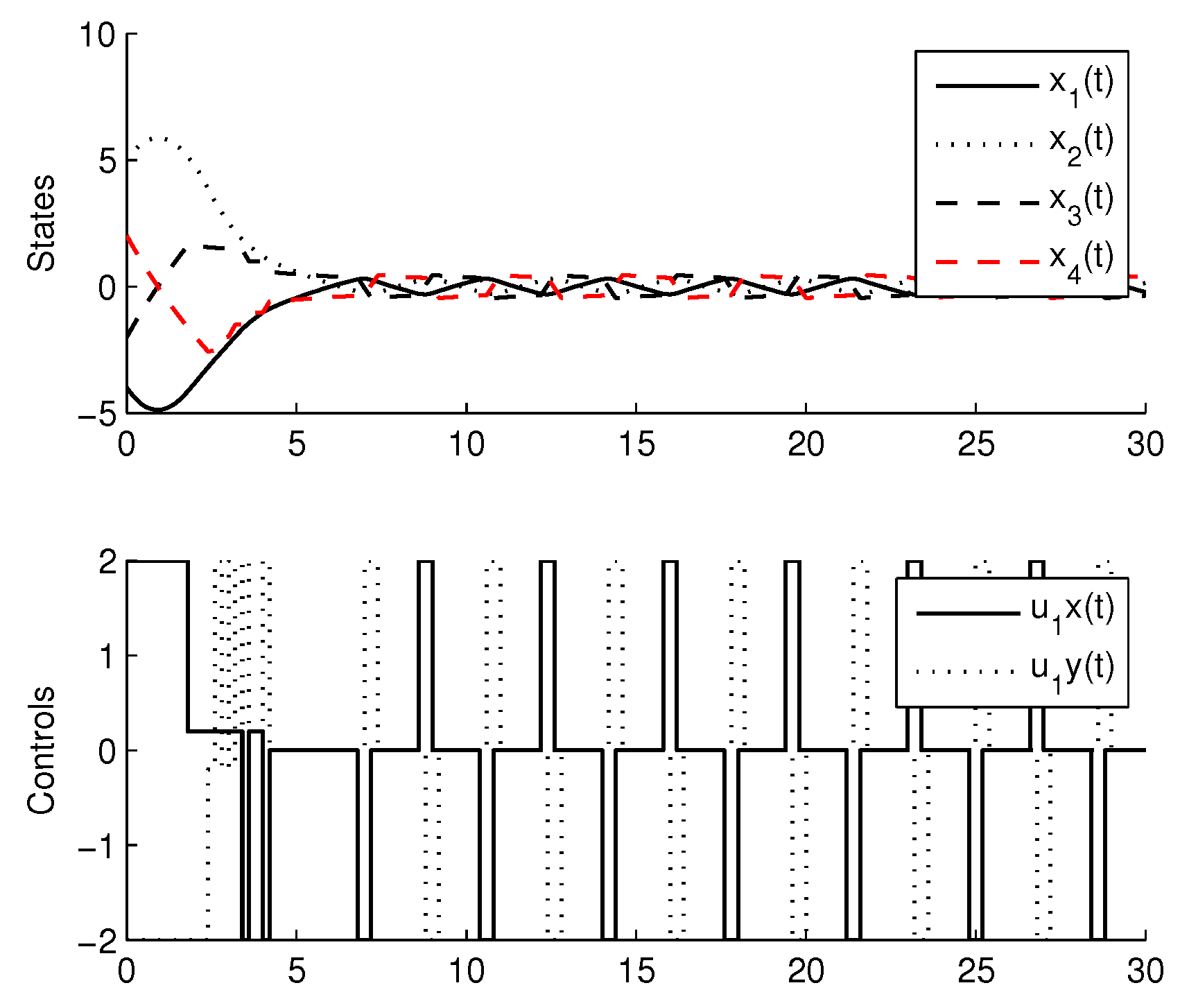
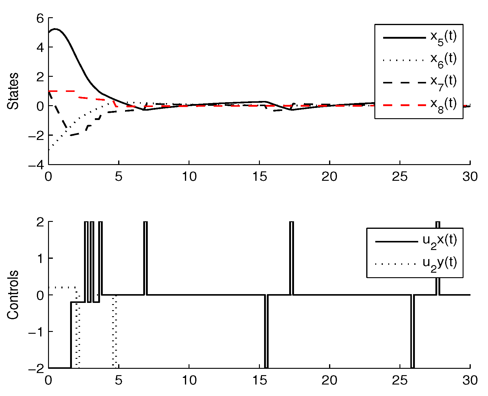
For the simulation, the learning parameters were set and the , the initial conditions for the experiment were set , the algorithm shows a convergence after 15 iterations, Figure 2 shows the states and the signal control for the agent 1, Figure 3 shows the states and the signal control for the agent 2. The final path followed by both agents are shown in Figure 4.
3.2. Experimental Set-up
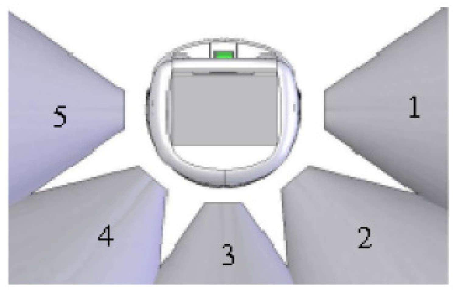
Two mobile robots Khepera IV are used to perform a experiment in MAS [42]. They have 5 sensors which are placed around the robot and are positioned and numbered as shown in Figure 5. These 5 sensors are ultrasonic devices compose of one transmitter and one receiver, they are used to detect the physical features of the environment such as obstacles and other nearby agents.
The five Khepera’s sonar readings are quantified in three degrees. They represent the amount of closeness to the nearest obstacle or others agents, 0 indicates obstacles or agents which are near, 1 indicates obstacles or agents which are in a medium distance and finally indicates obstacles or agents which are relatively far from the sensors.
The parameters (the distance to the target or the goal) and (the relative angle to the target or goal) are divided in eight degrees (0–8). Where 0 represents the smallest distance or angle and 8 represents the greatest relative distance or angle from the current Khepera’s position to the target or goal.
The actions available for the robot khepera are:
- Move forward
- Turn in clockwise direction
- Turn in counter clockwise direction
- Stand-Still
The ultra-sonic sensors on the Khepera are used to help the mobile robots to determine if there are any obstacles in the environment. The experimental set up reveals that the reinforcement learning algorithm relies strongly in the sensors readings.
Sensor readings in the ideal simulation situation are based on mathematical calculations which are accurate and consistent. In the experimental implementation the readings are inaccurate and fluctuating. During the application of the controller this effect is minimized by permitting a period after performing a joint action, with the above we ensure that the sensor has steady reading before it is recorded. In addition, by moving the robots at relatively slow step during the learning process, the collisions with other objects or agent are reduced. The quantified readings would be enough to represent the current location and velocity when the robots are moving [43].
3.3. Experimental Results
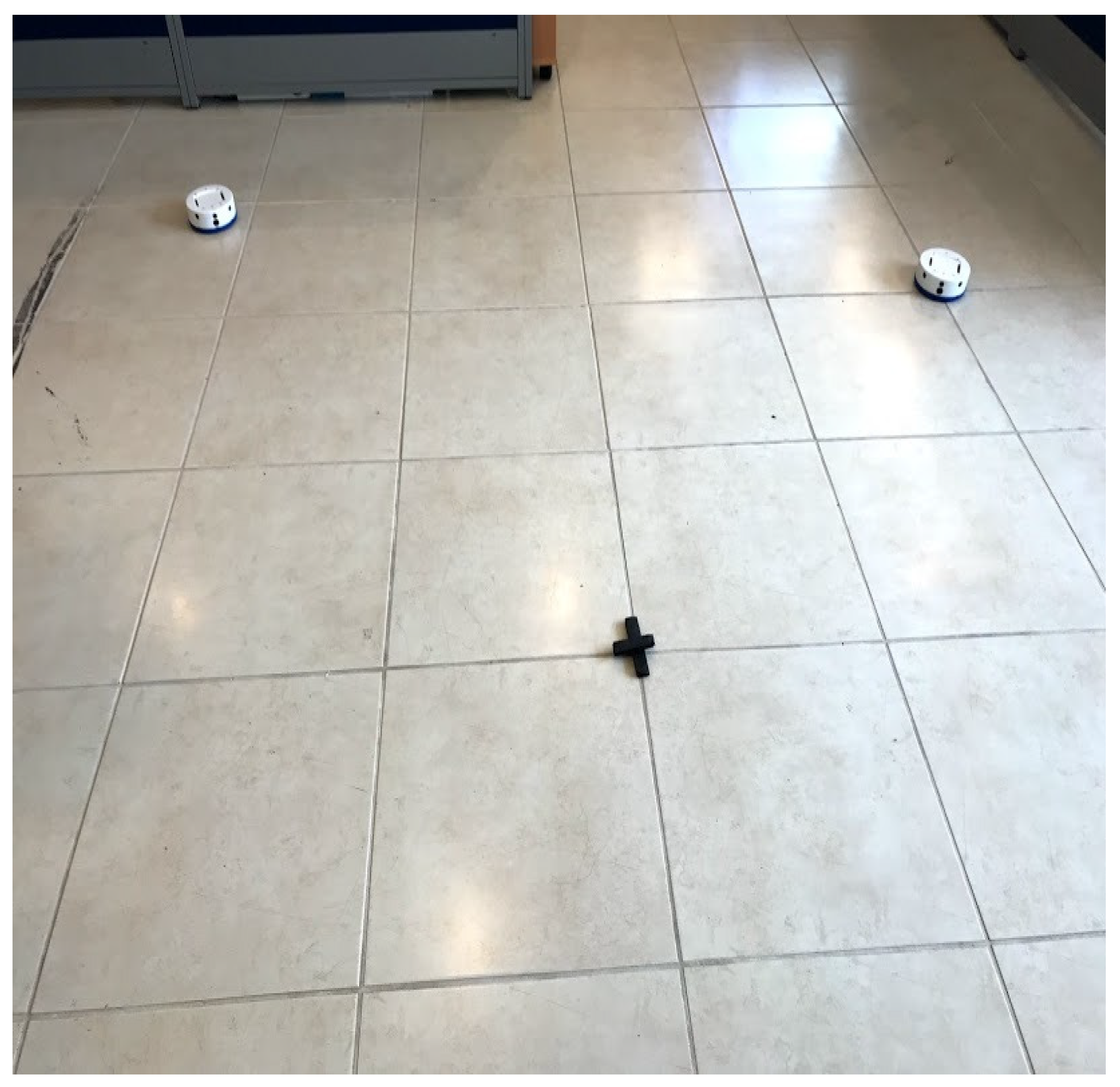
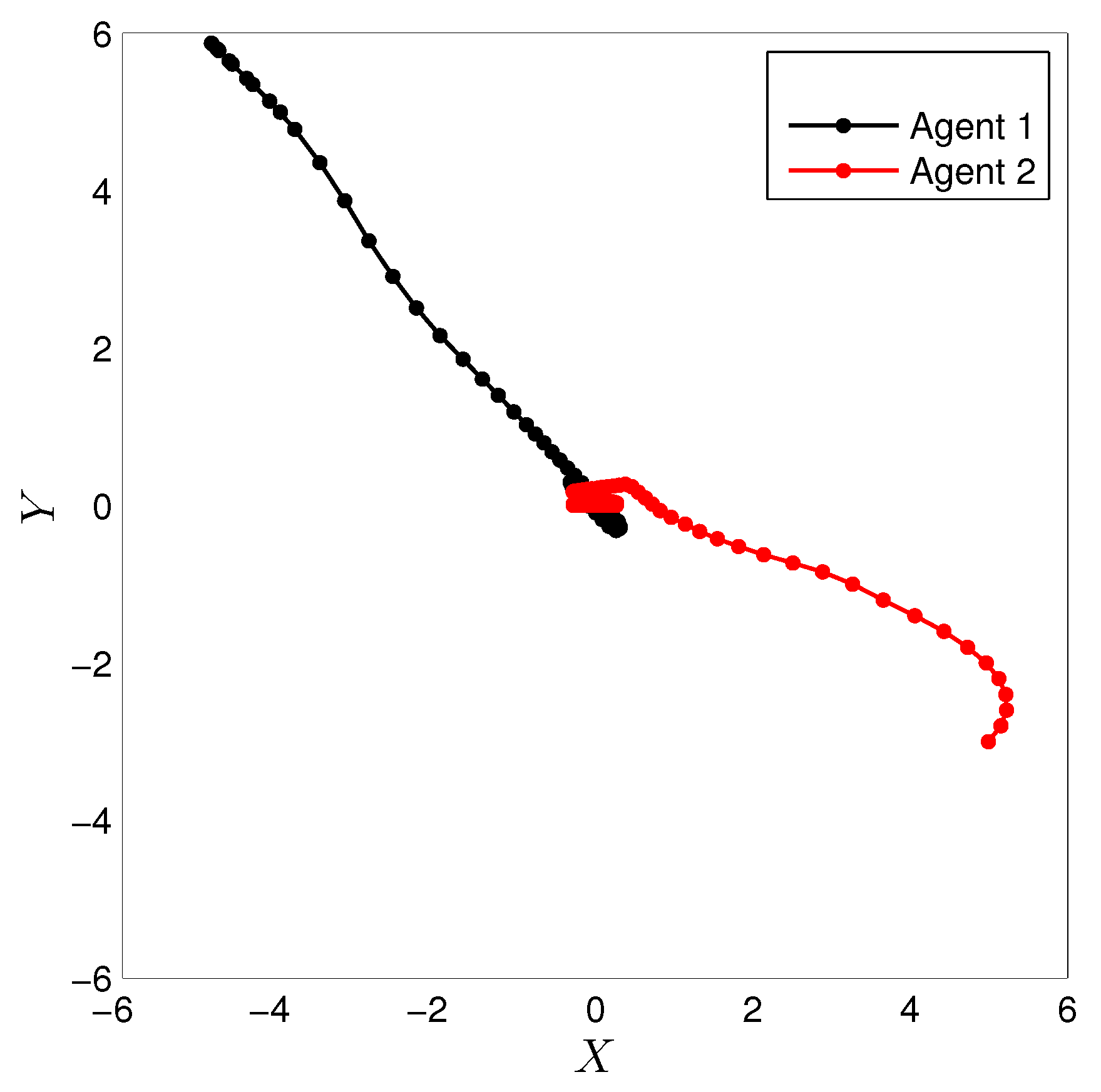
To validate the proposed algorithm, the linear fuzzy approximator of the joint Q-function is applied to a two-dimensional Multi-agent cooperative task. Two mobile robots Khepera IV must be driven in a surface such that both agents reach the origin at the same time with minimum time elapsed, it is shown in Figure 6.
The fuzzy partition and the location of centroids used for the states were the same as the simulation section.
The goal of arriving at the same moment toward the origin in minimum time elapsed is shown by the common reward function :
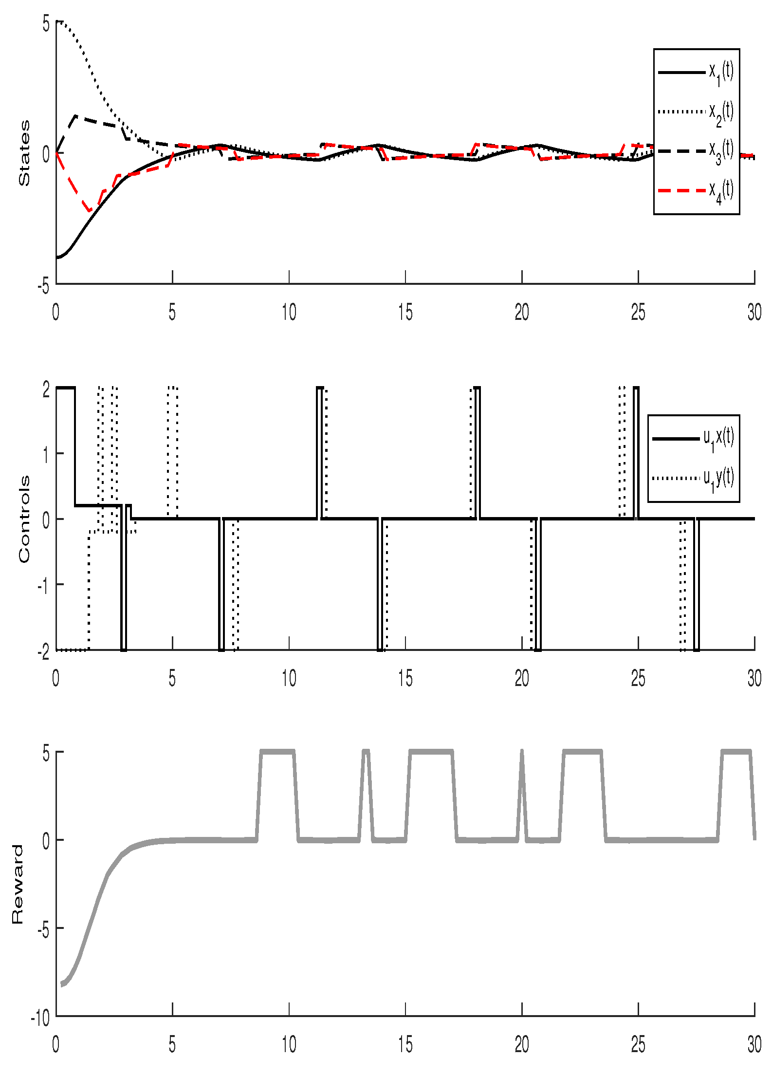
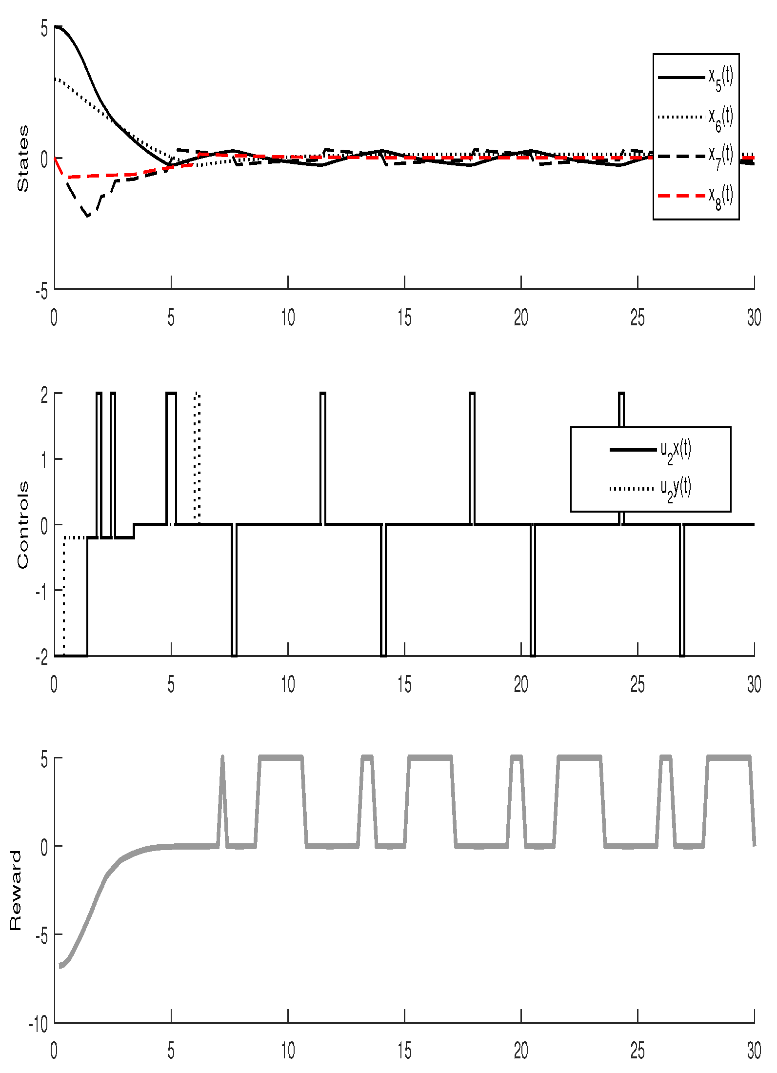
For this experiment the learning parameters were set and , the initial conditions for the experiment were set , the experiment shows a convergence after 27 iterations. Figure 7 shows the states, the signal control and the rewards for the agent 1 and Figure 8 shows the states, the signal control and the reward for the agent 2.
The election of the value for and was set arbitrarily, the vector converged after 27 iterations when the bounded was reached. The final path is shown in Figure 9, this trajectory is evidently different from the optimal policy, which would drive both agents in a straight line toward the goal since any initial position. However, with the fuzzy quantization used in this implementation and the effect of the damping, the final path obtained is the best that can be accomplished with this fuzzy parameterization. The coordination problem was overcame using an indirect method, where the agents learn to choose a solution by chance.
4. Comparison with CMOMMT Algorithm for Multi-Agent Systems
There are other methods for MARL in continuous state space, these proposals are restricted to a limited kind of task, one of this methods is “cooperative multi-robot observation of multiple moving target” (CMOMMT) given in [13], which relies in local information in order to learn cooperative behavior. It allows the application of the reinforcement learning in continuous state space for Multi-agents systems.
The kind of cooperation learned in this proposal is by implicit techniques, in this way this method is useful for reducing the representation of the state space through of a mapping of the continuous state space in a finite state space, where every new state discretized is considered as a region in the continuous state space.
The action space is discrete, this method uses a delayed reward where positive or negative values are obtained at the end of the training. Finally, an optimal joint policy of actions is obtained by a clustering technique in the discrete action space.
We performed the same cooperative task of arriving to the origin point at the same time for 2 agents as in the section above, using the same reward function and the same continuous state space. The initial condition was set .
The final path obtained by the CMOMMT algorithm is shown in Figure 10, where the path traced is not straight enough and near to the origin point is shown as a persistent oscillation. The signal state and the signal control for the agent 1 and agent 2 are shown in Figure 11 and the Figure 12, respectively.
The Table 1 shows a comparison between our proposal and the CMOMMT algorithm for an average of trials conducted under the same initial conditions.
One possible reason for the results of CMOMMT could be that the Q-functions obtained by this method are less smooth than the presented by the fuzzy parameterization. In this way the method proposed in our paper shows a better performance in the form of the more accuracy representation of the state space and less computational resources used by it.
5. Conclusions
One of the principal research direction of the artificial intelligent is to develop autonomous mobile robots with cooperative skills in continuous state space. For this reason, in this paper we have presented a linear fuzzy parameterization of the joint Q-function which is used with a modified version Q-learning algorithm. Our algorithm proposed can handle MARL problems with continuous state space, minimizing the time of convergence and avoiding storing the entire Q-values in a look up table. Triangular shapes were used to set the membership functions to define de estate space of the environment, this form was selected to simplify the projection mapping.
The main contribution of our work is that we present a reinforcement learning algorithm for MAS which uses a linear fuzzy parameterization of the joint Q-function. This approximation is carried out by means of a parameterization vector which only stores the Q-values at the centers of the triangular membership functions. The Q-values that are not found in the center are calculated by means of a weighted sum according to their degree of membership.
Two theorems were presented to guarantee the convergence to a fixed point in a finite number of iterations. The proposed method is a off-line model-based algorithm with deterministic dynamics, in the assumption that the joint reward function and the transition function are known by all the agents. Since having that kind of knowledge could be difficult in a real-life application, a future work could be to extend this proposal to a model free method, where the agents can learn by itself the dynamics of the environment, also this extension can be done to encompass problems with stochastic dynamics.
The performance of the linear fuzzy parameterization was evaluated first through simulation using Matlab software and then by an experiment where the task involves two mobile robots Khepera IV. Finally, the results obtained was compared with another suitable algorithm called CMOMMT which is capable of deal with tasks where the estate space is continuous.
Author Contributions
Formal analysis and Investigation D.L.-C.; Software, F.G.-L.; Validation, L.P.-D.; Review of the methods and editing, S.K.G.
Funding
The authors extend their appreciation to the Mexico’s Secretary of Public Education for funding this work through research agreement 511-6/17-7605.
Conflicts of Interest
The authors declare no conflict of interest. The founding sponsors had no role in the design of the study; in the collection, analyses, or interpretation of data; in the writing of the manuscript, and in the decision to publish the results.
References
- Sen, S.; Weiss, G. Multiagent Systems: A Modern Approach to Distributed Artificial Intelligence; MIT Press: Cambridge, MA, USA, 1999. [Google Scholar]
- Stone, P.; Veloso, M. Multiagent systems: A survey from machine learning perspective. Auton. Robots 2000, 8, 345–383. [Google Scholar] [CrossRef]
- Wooldridge, M. An Introduction to MultiAgent Systems; John Wiley & Sons: Hoboken, NL, USA, 2002. [Google Scholar]
- Rashid, A.T.; Ali, A.A.; Frasca, M.; Fortuna, L. Path planning with obstacle avoidance based on visibility binary tree algorithm. Robot. Auton. Syst. 2013, 61, 1440–1449. [Google Scholar] [CrossRef]
- Kaelbling, L.P.; Littman, M.L.; Moore, A.W. Reinforcement Learning: A Survey. J. Artif. Intell. Res. 1996, 4, 237–285. [Google Scholar] [CrossRef]
- Arel, I.; Liu, C.; Urbanik, T.; Kohls, A.G. Reinforcement learning-based multi-agent system for network traffic signal control. IET Intell. Transp. Syst. 2010, 4, 128–135. [Google Scholar] [CrossRef]
- Cherkassky, V.; Mulier, F. Learning from data: Concepts, Theory and Methods; Wiley-IEEE Press: Hoboken, NL, USA, 2007. [Google Scholar]
- Barlow, S.V. Unsupervised learning. In Unsupervised Learning: Foundations of Neural Computation, 1st ed.; Sejnowski, T.J., Hinton, G., Eds.; MIT Press: Cambridge, MA, USA, 1999; pp. 1–18. ISBN 9780262581684. [Google Scholar]
- Zhang, W.; Ma, L.; Li, X. Multi-agent reinforcement learning based on local communication. Clust. Comput. 2018, 1–10. [Google Scholar] [CrossRef]
- Hu, X.; Wang, Y. Consensus of Linear Multi-Agent Systems Subject to Actuator Saturation. Int. J. Control Autom. Syst. 2013, 11, 649–656. [Google Scholar] [CrossRef]
- Luviano, D.; Yu, W. Path planning in unknown environment with kernel smoothing and reinforcement learning for multi-agent systems. In Proceedings of the 12th International Conference on Electrical Engineering, Computing Science and Automatic Control (CCE), Mexico City, Mexico, 28–30 October 2015. [Google Scholar]
- Abul, O.; Polat, F.; Alhajj, R. Multi-agent reinforcement learning using function approximation. IEEE Trans. Syst. Man Cybern. Part C Appl. Rev. 2000, 485–497. [Google Scholar] [CrossRef]
- Fernandez, F.; Parker, L.E. Learning in large cooperative multi-robots systems. Int. J. Robot. Autom. Spec. Issue Comput. Intell. Tech. Coop. Robots 2001, 16, 217–226. [Google Scholar]
- Foerster, J.; Nardelli, N.; Farquhar, G.; Afouras, T.; Torr, P.H.; Kohli, P.; Whiteson, S. Stabilising experience replay for deep multi-agent reinforcement learning. arXiv, 2017; arXiv:1702.08887. [Google Scholar]
- Tamakoshi, H.; Ishi, S. Multi agent reinforcement learning applied to a chase problem in a continuous world. Artif. Life Robot. 2001, 202–206. [Google Scholar] [CrossRef]
- Ishiwaka, Y.; Sato, T.; Kakazu, Y. An approach to pursuit problem on a heterogeneous multiagent system using reinforcement learning. Robot. Auton. Syst. 2003, 43, 245–256. [Google Scholar] [CrossRef]
- Radac, M.-B.; Precup, R.-E.; Roman, R.-C. Data-driven model reference control of MIMO vertical tank systems with model-free VRFT and Q-Learning. ISA Trans. 2017. [Google Scholar] [CrossRef] [PubMed]
- Pandian, B.J.; Noel, M.M. Control of a bioreactor using a new partially supervised reinforcement learning algorithm. J. Process Control 2018, 69, 16–29. [Google Scholar] [CrossRef]
- Watkins, C.J.; Dayan, P. Q-learning. Mach. Learn. 1992, 8, 279–292. [Google Scholar] [CrossRef] [Green Version]
- Nguyen, T.; Nguyen, N.D.; Nahavandi, S. Multi-Agent Deep Reinforcement Learning with Human Strategies. arXiv, 2018; arXiv:1806.04562. [Google Scholar]
- Boutilier, C. Planning, Learning and Coordination in Multiagent Decision Processes. In Proceedings of the Sixth Conference on Theoretical Aspects of Rationality and Knowledge (TARK96), De Zeeuwse Stromen, The Netherlands, 17–20 March 1996; pp. 195–210. [Google Scholar]
- Harsanyi, J.C.; Selten, R. A General Theory of Equilibrium Selection in Games, 1st ed.; MIT Press: Cambridge, MA, USA, 1988; ISBN 9780262081733. [Google Scholar]
- Busoniu, L.; De Schutter, B.; Babuska, R. Decentralized Reinforcement Learning Control of a robotic Manipulator. In Proceedings of the International Conference on Control, Automation, Robotics and Vision, Singapore, 5–8 December 2006. [Google Scholar]
- Littman, M.L. Value-function reinforcement learning in Markov games. J. Cogn. Syst. Res. 2001, 2, 55–66. [Google Scholar] [CrossRef] [Green Version]
- Guestrin, C.; Lagoudakis, M.G.; Parr, R. Coordinated reinforcement learning. In Proceedings of the 19th International Conference on Machine Learning (ICML-2002), Sydney, Australia, 8–12 July 2002; pp. 227–234. [Google Scholar]
- Bowling, M.; Veloso, M. Multiagent learning using a variable learning rate. Artif. Intell. 2002, 136, 215–250. [Google Scholar] [CrossRef]
- Bertsekas, D.P. Dynamic Programming and optimal control vol. 2, 4th ed.; Athena Scientific: Belmont, MA, USA, 2017; ISBN 1-886529-44-2. [Google Scholar]
- Istratesku, V. Fixed Point Theory: An introduction; Springer: Berlin, Germany, 2002; ISBN 978-1-4020-0301-1. [Google Scholar]
- Melo, F.S.; Meyn, S.P.; Ribeiro, M.I. An analysis of reinforcement learning with functions approximation. In Proceedings of the 25th International Conference on Machine Learning (ICML-08), Helsinki, Finland, 5–9 July 2008; pp. 664–671. [Google Scholar]
- Szepesvari., C.; Smart, W.D. Interpolation-based Q-learning. In Proceedings of the 21st International Conference on Machine Learning (ICML-04), Banff, AB, Canada, 4–8 July 2004; pp. 791–798. [Google Scholar]
- Sutton, R.S.; McAllester, D.A.; Singh, S.P.; Mansour, Y. Policy gradient methods for reinforcement learning with function approximation. In Proceedings of the 12th International Conference on Neural Information Processing Systems, Denver, CO, USA, 29 November–4 December 1999; pp. 1057–1063. [Google Scholar]
- Bertsekas, D.P.; Tsitsiklis, J.N. Neuro-Dynamic Programming, 1st ed.; Athena Scientific: Belmont, MA, USA, 1996; ISBN 1-886529-10-8. [Google Scholar]
- Tsitsiklis, J.N.; Van Roy, B. Feature-based methods for large scale dynamic programming. Mach. Learn. 1996, 22, 59–94. [Google Scholar] [CrossRef] [Green Version]
- Kruse, R.; Gebhardt, J.E.; Klowon, F. Foundations of Fuzzy Systems, 1st ed.; John Wiley & Sons: Hoboken, NL, USA, 1994; ISBN 047194243X. [Google Scholar]
- Gordon, G.J. Reinforcement learning with function approximation converges to a region. Adv. Neural Inf. Process. Syst. 2001, 13, 1040–1046. [Google Scholar]
- Tsitsiklis, J.N. Asynchronous stochastic approximation and Q-learning. Mach. Learn. 1994, 16, 185–202. [Google Scholar] [CrossRef] [Green Version]
- Berenji, H.R.; Khedkar, P. Learning and tuning fuzzy logic controllers through reinforcements. IEEE Trans. Neural Netw. 1992, 3, 724–740. [Google Scholar] [CrossRef] [PubMed] [Green Version]
- Munos, R.; Moore, A. Variable-resolution discretization in optimal control. Mach. Learn. 2002, 49, 291–323. [Google Scholar] [CrossRef]
- Chow, C.S.; Tsitsiklis, J.N. An optimal one-way multi grid algorithm for discrete-time stochastic control. IEEE Trans. Autom. Control 1991, 36, 898–914. [Google Scholar] [CrossRef]
- Busoniu, L.; Ernst, D.; De Schutter, B.; Babuska, R. Approximate Dynamic programming with fuzzy parametrization. Automatica 2010, 46, 804–814. [Google Scholar] [CrossRef]
- Vlassis, N. A concise Introduction to Multi Agent Systems and Distributed Artificial Intelligence. In Synthesis Lectures in Artificial Intelligence and Machine Learning; Morgan & Claypool Publishers: San Rafael, CA, USA, 2007. [Google Scholar]
- K-Team Corporation. 2013. Available online: http://www-k-team.com (accessed on 15 January 2018).
- Ganapathy, V.; Soh, C.Y.; Lui, W.L.D. Utilization of webots and Khepera II as a Platform for neural Q-learning controllers. In Proceedings of the IEEE Symposium on Industrial Electronics and Applications, Kuala Lumpur, Malaysia, 25–27 May 2009. [Google Scholar]
Figure 1.
Triangular fuzzy partition for velocity state.

Figure 2.
States and signal control for the Agent 1.

Figure 3.
States and signal control for Agent 2.

Figure 4.
Final path by Agent 1 and Agent 2.

Figure 5.
Position of the Khepera’s UltraSonic sensors.

Figure 6.
Experimental test

Figure 7.
States and Rewards for the Agent 1 in the experimental implementation.

Figure 8.
States and Rewards for the Agent 2 in the experimental implementation.

Figure 9.
Final path by Agent 1 and Agent 2 in experimental implementation.

Figure 10.
Final path obtained by CMOMMT algorithm.

Figure 11.
States and signal control for agent 1 CMOMMT algorithm.

Figure 12.
States and signal control for agent 2 CMOMMT algorithm.


Table 1.
Comparison between fuzzy partition and CMOMMT.
| Training | CMOMMT | Fuzzy Parameterization |
|---|---|---|
| Error (cm) | 18 | 6 |
| Time (s) | 25 | 12 |
| Iterations | 34 | 27 |
© 2018 by the authors. Licensee MDPI, Basel, Switzerland. This article is an open access article distributed under the terms and conditions of the Creative Commons Attribution (CC BY) license (http://creativecommons.org/licenses/by/4.0/).
Share and Cite
MDPI and ACS Style
Luviano-Cruz, D.; Garcia-Luna, F.; Pérez-Domínguez, L.; Gadi, S.K. Multi-Agent Reinforcement Learning Using Linear Fuzzy Model Applied to Cooperative Mobile Robots. Symmetry 2018, 10, 461. https://doi.org/10.3390/sym10100461
AMA Style
Luviano-Cruz D, Garcia-Luna F, Pérez-Domínguez L, Gadi SK. Multi-Agent Reinforcement Learning Using Linear Fuzzy Model Applied to Cooperative Mobile Robots. Symmetry. 2018; 10(10):461. https://doi.org/10.3390/sym10100461
Chicago/Turabian StyleLuviano-Cruz, David, Francesco Garcia-Luna, Luis Pérez-Domínguez, and S. K. Gadi. 2018. "Multi-Agent Reinforcement Learning Using Linear Fuzzy Model Applied to Cooperative Mobile Robots" Symmetry 10, no. 10: 461. https://doi.org/10.3390/sym10100461
Note that from the first issue of 2016, this journal uses article numbers instead of page numbers. See further details here.