Symmetric Triangular Interval Type-2 Intuitionistic Fuzzy Sets with Their Applications in Multi Criteria Decision Making

Abstract

Type-2 intuitionistic fuzzy set (T2IFS) is a powerful and important extension of the classical fuzzy set, intuitionistic fuzzy set to measure the vagueness and uncertainty. In a practical decision-making process, there always occurs an inter-relationship among the multi-input arguments. To deal with this point, the motivation of the present paper is to develop some new interval type-2 (IT2) intuitionistic fuzzy aggregation operators which can consider the multi interaction between the input argument. To achieve it, we define a symmetric triangular interval T2IFS (TIT2IFS), its operations, Hamy mean (HM) operator to aggregate the preference of the symmetric TIT2IFS and then shows its applicability through a multi-criteria decision making (MCDM). Several enviable properties and particular cases together with following different parameter values of this operator are calculated in detail. At last a numerical illustration is to given to exemplify the practicability of the proposed technique and a comparative analysis is analyzed in detail.

1. Introduction

Multiple criteria decision making (MCDM) is a hot research topic in the modern decision-making process to find the most suitable alternative(s) from the available ones. In this process, all the alternatives are to be evaluated under several attributes by both qualitatively and quantitatively [1,2]. Traditionally, the researchers offer his/her preference information towards the alternatives by using the crisp real numbers only. However, due to lack of knowledge, a time pressure, and other unavoidable factors, it is very difficult if not impossible to express the information precisely. Therefore, to handle the incomplete or incorrect information, the theory of fuzzy set (FS) also called as a type-1 fuzzy set (T1FS) [3] and its extensions as an intuitionistic FS (IFS) [4], type-2 FS (T2FS) [5] are widely used. Under these environments, authors have put forth the different techniques to solve the MCDM problems. For instance, geometric aggregation operators (AOs) for different intuitionistic fuzzy numbers (IFNs) are developed by Xu and Yager [6]. Garg [7,8] presented some Einstein norm based AOs for IFNs. Zhao et al. [9] presented some generalized AOs. Kaur and Garg [10] presented some generalized AOs using t-norm operations for cubic IFS information. However, apart from these, a comprehensive overview of the different approaches for solving the decision making (DM) problems by using aggregation operator (AOs) [11,12,13,14,15,16,17,18,19,20,21], information measures (IMs) [22,23,24] are summarized in these papers and their references.

In these existing works, authors have investigated the problem by taking quantitative environment to access the alternatives. However, not all the alternatives are accessed in terms of quantitative. For this, there exists the concept of qualitative assessment in terms of linguistic variables/terms (LVs/LTs) [25,26]. By taking the advantages of LTs, Zhang [27] presented the linguistic IF (LIF) AOs to aggregate the LIF numbers. Chen et al. [28] presented an approach to solving the MCDM problem under LIFS environment. Garg and Kumar [29] presented AOs for LIF numbers (LIFNs) by using set pair analysis theory. Garg and Kumar [30] presented new possibility degree measure for LIFNs and an AO to aggregate the different LIFNs to solve MCDM problems. In many practical problems, it is not easy for any decision maker (DM) to discover an exact membership function of an FS corresponding to its element. To overthrow this limitation, type-2 fuzzy set (T2FS), an extension of T1FS, is applied to the model and is characterized by two functions: primary membership functions (PMF) and secondary membership function (SMF). Unfortunately, T2FSs are highly complex, it is troublesome for the DMs to implement it in the real situation; hence, their use is not yet widespread. To reduce the computational complexity, Interval type-2 fuzzy (IT2F) sets (IT2FSs) [31] is the most widely used in T2FSs. In past decades, many methods have been developed to extend the theory of MCDM under IT2FS environment. Chen et al. [32] built up an expanded QUALIFLEX strategy for taking care of DM issues in view of IT2FSs and gave a contextual analysis of medicinal basic leadership. Chen [33] built up an ELECTRE-base outranking strategy for decision-making problems using IT2FSs. Wu and Mendel [34] proposed a linguistic weighted average AOs to deal with analytical hierarchical process (AHP) process under IT2F environment. Qin and Liu [35] investigated a family of type-2 fuzzy AOs in light of Frank triangular norm and built up another way to deal with MCDM problems under the IT2FSs setting. Gong et al. [36] extended the generalized Bonferroni mean (GBM) operator to the trapezoidal IT2F environment. Apart from these, some other studies under T2FS environment are conducted which are summarized in [35,36,37,38,39,40,41,42,43,44,45,46,47,48].

In all these above AOs, researchers have described the information by considering the independent of argument assumptions during the aggregation. However, the interaction between the multi-input parameters have commonly occurred and thus, it is necessary to add their features into the process. In that direction, Bonferroni mean (BM) and generalized BM (GBM)-based operators are proposed by the researchers [49,50]. But from them, it has been observed that they have considered only two or three multi-parameter at a single time. However, they are unable to analyze the effect of the multi-input argument into one analysis. Furthermore, in BM and GBM, there is a need for two and three parameters from the irrational set during the process which increases the computational complexity. An alternative to BM operators, Hamy mean (HM) [51] or Maclaurin symmetric mean (MSM) or Muirhead mean (MM) operator has advantages of capturing the inter-relationship among the multiple input arguments. Qin [46] make a correlation between the HM and the MSM and conclude that the MSM is an instance of HM [16,17]. Garg and Nancy [52] develop MCDM method by prioritized MM aggregation operators. Additionally, the HM operator involves the parameter, which can provide more flexibility and robustness during the aggregation operator. The existing - arithmetic and geometric mean- operators can be easily deduced from the HM by setting a particular value to its parameter. Be that as it may, the HM just accomplished a couple of research results on the hypothesis and application of inequality [53,54]. Therefore, it is a means to study the AOs using the HM operator.

It is noted from the above studies that T2FS or IT2FS are examined by considering only the membership degree (MD) of an element. But in practical problems, it is sometimes not possible for a DM to give their preferences in terms of MD only as there may be some amount of hesitation also. For discussing this, a type-2 IFS (T2IFS) [39] has been introduced which simultaneously considers the MDs, non-membership degrees (NMDs) and the footprint of uncertainties (FOU) between them. Later on, due to the high complexity of T2IFS, Garg and Singh [55] introduced the concept of triangular interval T2IFS (TIT2IFS) has introduced by considering the MDs and NMDs as a triangular fuzzy number.

Based on the above analysis, we can know that the decision-making problems have become more tedious these days. So in order to make a better decision in terms of selecting the best alternative(s) for the MCDM problems, it is necessary to consider the various factors such as MDs, NMDs, FOU between the alternatives. By keeping the advantages of both the AOs and the TIT2IFS, it is necessary to extend the Hamy mean AOs to process the TIT2IFNs by using linguistic features of MDs and NMDs and hence to develop some MCDM methods. Until now, we have not seen any work based on the AOs used to aggregate the TIT2IFS information. Thus, keeping in mind the advantages of T2IFS and the multiple input interaction between the argument of HM operator, this paper has presented the concept of the symmetric TIT2IFS and their desired properties. These considerations have led us to consider the main objectives of this paper:

• to propose the concept of the symmetric TIT2IFS (STIT2IFSs);
• to propose some new AOs for STIT2IFSs under the linguistic intuitionistic features;
• to develop an algorithm to solve the decision-making problems based on proposed operators;
• to present some example to validate and compare the results.

To achieve the objective (1), we combine the T2IFSs and the symmetric triangular number to build a concept of the STIT2IFSs and studied their desired properties. To complete the objective (2), we presented the averaging AOs by using HM operations and named as symmetric triangular IT2IF HM averaging (STIT2IFHM) and weighted symmetric triangular IT2IF Hamy mean averaging (WSTIT2IFHM) operator for decision-making problems by keeping in mind the advantages of T2IFS and the multiple input interaction between the argument of HM operator. Several enviable properties and particular cases together with following different parameter values of this operator are calculated in detail. To cover the objective (3), we establish an MCDM method based on these proposed operators under the STIT2IFS environment where preferences related to each alternative is expressed in terms of linguistic STIT2IFNs. A numerical illustration is to given to exemplify the practicability of the proposed technique and a comparative analysis is analyzed in detail for fulfilling the Objective 4. Finally, the advantages of the proposed method in the state of the art are highlighted and discussed in detail.

The rest of the paper is organized as follows. In Section 2, some basic concepts on T2FS, IT2FS, T2IFS, and HM are reviewed briefly. In Section 3, we present the concept of the symmetric TIT2IF set and their desirable properties. Section 4 deals with new AOs based on HM operator to accommodate the STIT2IFN information and its special cases. In Section 5, we present an approach based on the WSTIT2IFHM operator to solve the MCDM problem. A practical example is discussed in Section 6 and some concluding remarks are summarized in Section 7.

2. Basic Concepts

In this section, we overview some basic definition of T2FSs, IT2FS and T2IFSs defined over the universal set X.

Definition 1 ([42]).

A type-2 fuzzy set (T2FS) $A\subseteq X$, defined as

$$\begin{array}{c}\hfill A=\{((x,u_A),{\mu }_A(x,u_A))\mid x\in X,u_A\in j_x\subseteq [0,1]\}\end{array}$$

(1)

where $u_A$ denotes the primary membership function (PMF) of A, ${\mu }_A\in [0,1]$ is called as secondary membership function (SMF) $j_x\subseteq [0,1]$ is PMF of x.

Another equivalent expression for T2FS A is given as

$$\begin{array}{c}\hfill A={\int }_{x\in X}{\displaystyle \frac{{\mu }_A\left(x\right)}{x}}={\int }_{x\in X}\left[{\int }_{u_A\in j_x}{\displaystyle \frac{\left(f_x\left(u_A\right)\right)}{u_A}}\right]/x\end{array}$$

(2)

Definition 2 ([20]).

The collection of all PMFs of T2FS is named as “footprint of uncertainty" (FOU), i.e., $FOU\left(A\right)={\displaystyle \bigcup _{x\in X}}{j}_x$.

However, because of high computational burden of T2FSs, researchers prefer using interval type-2 (IT2) fuzzy set (IT2FS) for real-world problems.

Definition 3 ([44]).

A T2FS transform into interval type-2 FS when the grades of all SMFs is equal to 1. Mathematically, an IT2FS A, with a membership function ${\mu }_A(x,u_A)$, may be expressed either as Equation (3) or as Equation (4):

$$\begin{array}{ccc}\hfill A& =& \{(x,u_A),{\mu }_A(x,u_A)=1\mid \forall x\in X,\forall u_A\in j_x\subseteq [0,1]\}\hfill \end{array}$$

(3)

$$\begin{array}{ccc}\hfill A& =& {\int }_{x\in X}{\int }_{u_A\in j_x}1/(x,u_A),j_x\subseteq [0,1]\hfill \end{array}$$

(4)

Definition 4 ([44]).

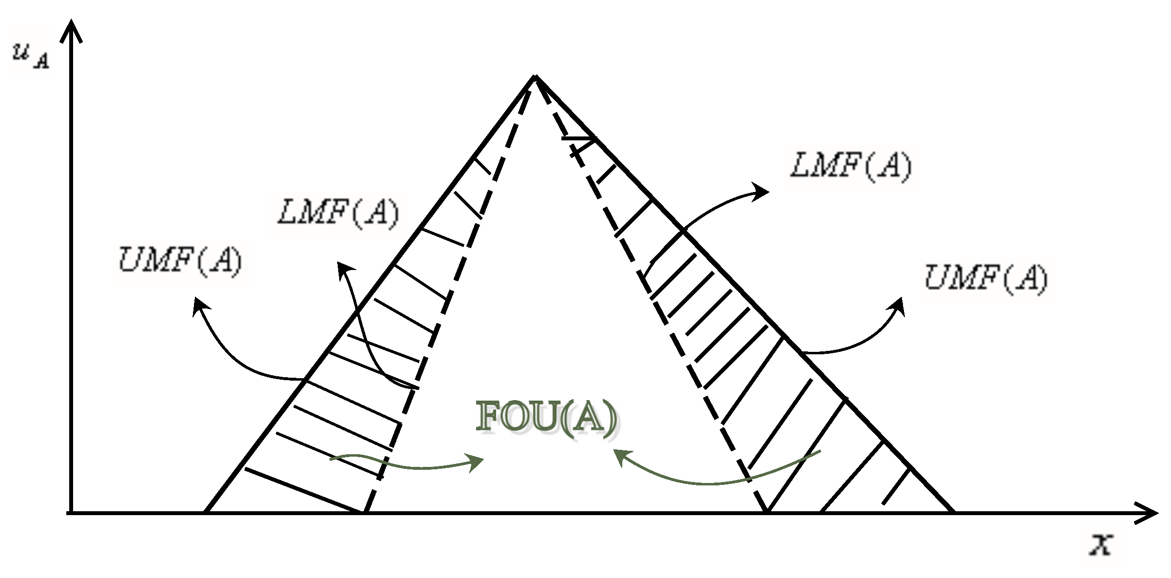
An IT2 FS is normally described by a zone called as FOU, which is limited by two membership functions (MFs), known as lower MF (LMF) ${\underline{\mu }}_A(x,u_A)$ and the upper MF (UMF) ${\overline{\mu }}_A(x,u_A)$. That is FOU=[${\underline{\mu }}_A(x,u_A),{\overline{\mu }}_A(x,u_A)$]. Figure 1 shows the graphical representation of IT2 fuzzy number (IT2 FN) with triangular MF shape.

Definition 5 ([38,39]).

A T2IFS is a set of ordered pairs consisting of PMFs and SMFs of the element defined as

$$\begin{array}{c}\hfill A=\left\{\langle (x,u_A,v_A),{\mu }_A(x,u_A),{\nu }_A(x,v_A)\rangle \mid x\in X,u_A\in j_x^1,v_A\in j_x^2\right\}\end{array}$$

(5)

where $u_A\left(v_A\right)$ represents the primary membership (non-membership) of A denoted by PMF(PNMF), ${\mu }_A\left({\nu }_A\right)$ is secondary membership (non-membership) function of A, denoted by SMF (SNMF) and $j_x^1,j_x^2\subseteq [0,1]$ are PMF and PNMF of x, respectively. When the SMFs ${\mu }_A(x,u_A)=1$, and SNMF ${\nu }_A(x,v_A)=0$, a T2IFS translates to an IT2 IFS.

Definition 6 ([55]).

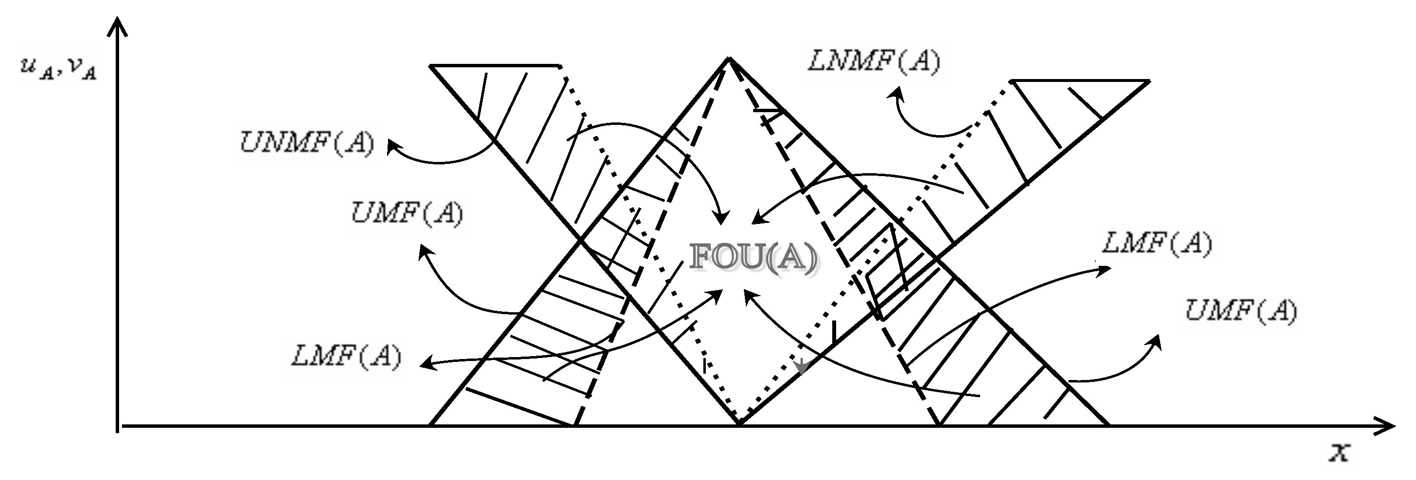
An IT2 IFS, A, is described by a bounding functions of lower and upper membership and non-membership functions denoted by LMF, UMF, LNMF and UNMF defined as ${\overline{\mu }}_A$, ${\underline{\mu }}_A$ and ${\overline{\nu }}_A$, ${\underline{\nu }}_A$ with conditions: $0\le {\overline{\mu }}_A+{\underline{\nu }}_A\le 1$ and $0\le {\underline{\mu }}_A+{\overline{\nu }}_A\le 1$. The FOUs of an IT2IFS is illustrated in Figure 2 with triangular shape and defined mathematically as

$$\begin{array}{c}\hfill FOU\left(A\right)=\bigcup _{x\in X}\left[{\underline{\mu }}_A\left(x\right),{\overline{\mu }}_A\left(x\right),{\underline{\nu }}_A\left(x\right),{\overline{\nu }}_A\left(x\right)\right]\end{array}$$

Definition 7 ([51]).

For non-negative real numbers $x_i(i=1,2,\dots ,n)$, the Hamy mean (HM) is given as

$$\begin{array}{c}\hfill {HM}^{\left(k\right)}(x_1,x_2,\cdots ,x_n)={\displaystyle \frac{{\displaystyle \sum _{\genfrac{}{}{0pt}{}{1\le i_1<}{\dots <i_k\le n}}}{\left({\displaystyle \prod _{j=1}^k}{x}_{i_j}\right)}^{\frac{1}{k}}}{\left(\genfrac{}{}{0pt}{}{n}{k}\right)}}\end{array}$$

(6)

where k is the parameter, $\left(\genfrac{}{}{0pt}{}{n}{k}\right)=\frac{n!}{k!(n-k)!}$ and $(i_1,i_2,\dots ,i_k)$ crosses all the $k-$tuple mix of $(1,2,\dots ,n)$.

3. Proposed Symmetric Triangular Interval T2IFS

In this section, we present a symmetric triangular IT2IFS and characterize their fundamental operational laws.

Definition 8.

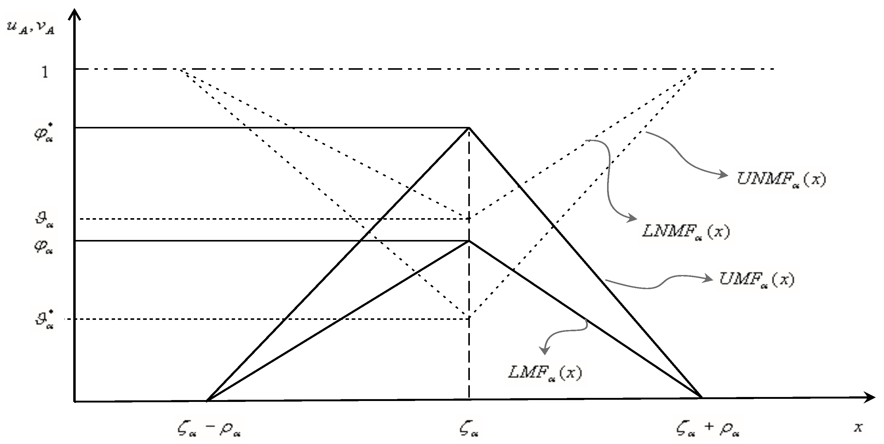
Let X be the universal set. A symmetric triangular interval T2 IFS (TIT2IFS) can be represented as follows:

$$\begin{array}{c}\hfill \alpha =\left\{\left({\zeta }_{\alpha }\left(x\right),{\varrho }_{\alpha }\left(x\right),{\phi }_{\alpha }\left(x\right),{\phi }_{\alpha }^{\ast }\left(x\right),{\vartheta }_{\alpha }\left(x\right),{\vartheta }_{\alpha }^{\ast }\left(x\right)\right)\mid x\in X\right\}\end{array}$$

(7)

where ${\zeta }_{\alpha }\left(x\right),{\varrho }_{\alpha }\left(x\right),{\phi }_{\alpha }\left(x\right),{\phi }_{\alpha }^{\ast }\left(x\right)$, ${\vartheta }_{\alpha }\left(x\right),{\vartheta }_{\alpha }^{\ast }\left(x\right)$ are the real numbers satisfying the inequalities, ${\zeta }_{\alpha }\left(x\right)\ge {\varrho }_{\alpha }\left(x\right)$, $0\le {\phi }_{\alpha }\left(x\right)\le {\phi }_{\alpha }^{\ast }\left(x\right)\le 1$, $0\le {\vartheta }_{\alpha }^{\ast }\left(x\right)\le {\vartheta }_{\alpha }\left(x\right)\le 1$ such that ${\phi }_{\alpha }\left(x\right)+{\vartheta }_{\alpha }\left(x\right)\le 1$ and ${\phi }_{\alpha }^{\ast }\left(x\right)+{\vartheta }_{\alpha }^{\ast }\left(x\right)\le 1$.

For convenience, we represent this pair as $\alpha =\left({\zeta }_{\alpha },{\varrho }_{\alpha },{\phi }_{\alpha },{\phi }_{\alpha }^{\ast },{\vartheta }_{\alpha },{\vartheta }_{\alpha }^{\ast }\right)$ and called as symmetric triangular IT2 intuitionistic fuzzy (IT2IF) number (STIT2IFN) where ${\zeta }_{\alpha }\ge {\varrho }_{\alpha }$, ${\phi }_{\alpha }+{\vartheta }_{\alpha }\le 1$, ${\phi }_{\alpha }^{\ast }+{\vartheta }_{\alpha }^{\ast }\le 1$ and ${\phi }_{\alpha }\le {\phi }_{\alpha }^{\ast }$, ${\vartheta }_{\alpha }\ge {\vartheta }_{\alpha }^{\ast }$. The graphical representation of STIT2IFN is given in Figure 3.

Definition 9.

For a STIT2IFN $\alpha =\left({\zeta }_{\alpha },{\varrho }_{\alpha },{\phi }_{\alpha },{\phi }_{\alpha }^{\ast },{\vartheta }_{\alpha },{\vartheta }_{\alpha }^{\ast }\right)$, the lower and upper membership and non-membership functions denoted by LMF, UMF, LNMF and UNMF are defined as

$$\begin{array}{c}\hfill {UMF}_{\alpha }\left(x\right)=\left\{\begin{array}{cc}{\displaystyle \frac{{\phi }_{\alpha }^{\ast }}{{\varrho }_{\alpha }}}(x-{\zeta }_{\alpha }+{\varrho }_{\alpha }),\hfill & {\zeta }_{\alpha }-{\varrho }_{\alpha }\le x<{\zeta }_{\alpha }\hfill \\ {\phi }_{\alpha }^{\ast },\hfill & x={\zeta }_{\alpha }\hfill \\ {\displaystyle \frac{{\phi }_{\alpha }^{\ast }}{{\varrho }_{\alpha }}}({\zeta }_{\alpha }+{\varrho }_{\alpha }-x),\hfill & {\zeta }_{\alpha }<x\le {\varrho }_{\alpha }+{\zeta }_{\alpha }\hfill \end{array}\right.;{UNMF}_{\alpha }\left(x\right)=\left\{\begin{array}{cc}{\displaystyle \frac{({\vartheta }_{\alpha }^{\ast }-1)(x-{\zeta }_{\alpha }+{\varrho }_{\alpha })+{\varrho }_{\alpha }}{{\varrho }_{\alpha }}};\hfill & {\zeta }_{\alpha }-{\varrho }_{\alpha }\le x<{\zeta }_{\alpha }\hfill \\ {\vartheta }_{\alpha }^{\ast };\hfill & x={\zeta }_{\alpha }\hfill \\ {\displaystyle \frac{(1-{\vartheta }_{\alpha }^{\ast })(x-{\zeta }_{\alpha })+{\vartheta }_{\alpha }^{\ast }{\varrho }_{\alpha }}{{\varrho }_{\alpha }}};\hfill & {\zeta }_{\alpha }<x\le {\varrho }_{\alpha }+{\zeta }_{\alpha }\hfill \end{array}\right.\end{array}$$

(8)

$$\begin{array}{c}\hfill {LMF}_{\alpha }\left(x\right)=\left\{\begin{array}{cc}{\displaystyle \frac{{\phi }_{\alpha }}{{\varrho }_{\alpha }}}(x-{\zeta }_{\alpha }+{\varrho }_{\alpha });\hfill & {\zeta }_{\alpha }-{\varrho }_{\alpha }\le x<{\zeta }_{\alpha }\hfill \\ {\phi }_{\alpha };\hfill & x={\zeta }_{\alpha }\hfill \\ {\displaystyle \frac{{\phi }_{\alpha }}{{\varrho }_{\alpha }}}({\zeta }_{\alpha }+{\varrho }_{\alpha }-x);\hfill & {\zeta }_{\alpha }<x\le {\varrho }_{\alpha }+{\zeta }_{\alpha }\hfill \end{array}\right.;{LNMF}_{\alpha }\left(x\right)=\left\{\begin{array}{cc}{\displaystyle \frac{({\vartheta }_{\alpha }-1)(x-{\zeta }_{\alpha }+{\varrho }_{\alpha })+{\varrho }_{\alpha }}{{\varrho }_{\alpha }}};\hfill & {\zeta }_{\alpha }-{\varrho }_{\alpha }\le x<{\zeta }_{\alpha }\hfill \\ {\vartheta }_{\alpha };\hfill & x={\zeta }_{\alpha }\hfill \\ {\displaystyle \frac{(1-{\vartheta }_{\alpha })(x-{\zeta }_{\alpha })+{\vartheta }_{\alpha }{\varrho }_{\alpha }}{{\varrho }_{\alpha }}};\hfill & {\zeta }_{\alpha }<x\le {\varrho }_{\alpha }+{\zeta }_{\alpha }\hfill \end{array}\right.\end{array}$$

(9)

Definition 10.

The score function of STIT2IFN $\alpha =\left({\zeta }_{\alpha },{\varrho }_{\alpha },{\phi }_{\alpha },{\phi }_{\alpha }^{\ast },{\vartheta }_{\alpha },{\vartheta }_{\alpha }^{\ast }\right)$ is defined as

$$\begin{array}{ccc}\hfill s\left(\alpha \right)& =& (s_x\left(\alpha \right),s_y\left(\alpha \right))\hfill \\ & =& \left({\zeta }_{\alpha }{\displaystyle \frac{2{\phi }_{\alpha }{\phi }_{\alpha }^{\ast }}{{\phi }_{\alpha }+{\phi }_{\alpha }^{\ast }}}-{\zeta }_{\alpha }{\displaystyle \frac{2{\vartheta }_{\alpha }{\vartheta }_{\alpha }^{\ast }}{{\vartheta }_{\alpha }+{\vartheta }_{\alpha }^{\ast }}},{\displaystyle \frac{{\vartheta }_{\alpha }+{\phi }_{\alpha }^{\ast }}{2}}-{\displaystyle \frac{{\phi }_{\alpha }+{\vartheta }_{\alpha }^{\ast }}{2}}\right)\hfill \end{array}$$

(10)

Definition 11.

For two STIT2IFNs α and β, an order relation “$(>)$” to compare them is defined as

• If $s_x\left(\alpha \right)>s_x\left(\beta \right)$, then $\alpha >\beta$;
• If $s_x\left(\alpha \right)=s_x\left(\beta \right),then\left\{\begin{array}{cc}{s}_y\left(\alpha \right)>s_y\left(\beta \right)\hfill & \Rightarrow \alpha >\beta ;\hfill \\ s_y\left(\alpha \right)=s_y\left(\beta \right)\hfill & \Rightarrow \alpha =\beta ;\hfill \end{array}\right.$

Definition 12.

For two STIT2IFNs $\alpha =\left({\zeta }_{\alpha },{\varrho }_{\alpha },{\phi }_{\alpha },{\phi }_{\alpha }^{\ast },{\vartheta }_{\alpha },{\vartheta }_{\alpha }^{\ast }\right)$ and $\beta =\left({\zeta }_{\beta },{\varrho }_{\beta },{\phi }_{\beta },{\phi }_{\beta }^{\ast },{\vartheta }_{\beta },{\vartheta }_{\beta }^{\ast }\right)$, $\lambda >0$, then the operational laws of it are shown as follows:

• $\alpha \oplus \beta =\left(\begin{array}{c}\hfill {\zeta }_{\alpha }+{\zeta }_{\beta },{\varrho }_{\alpha }+{\varrho }_{\beta },{\phi }_{\alpha }{\phi }_{\beta },{\phi }_{\alpha }^{\ast }+{\phi }_{\beta }^{\ast }-{\phi }_{\alpha }^{\ast }{\phi }_{\beta }^{\ast },{\vartheta }_{\alpha }+{\vartheta }_{\beta }-{\vartheta }_{\alpha }{\vartheta }_{\beta },{\vartheta }_{\alpha }^{\ast }{\vartheta }_{\beta }^{\ast }\end{array}\right)$;
• $\alpha \otimes \beta =\left(\begin{array}{c}\hfill {\zeta }_{\alpha }{\zeta }_{\beta },{\varrho }_{\alpha }{\varrho }_{\beta },{\phi }_{\alpha }+{\phi }_{\beta }-{\phi }_{\alpha }{\phi }_{\beta },{\phi }_{\alpha }^{\ast }{\phi }_{\beta }^{\ast },{\vartheta }_{\alpha }{\vartheta }_{\beta },{\vartheta }_{\alpha }^{\ast }+{\vartheta }_{\beta }^{\ast }-{\vartheta }_{\alpha }^{\ast }{\vartheta }_{\beta }^{\ast }\end{array}\right)$;
• $\lambda \alpha =\left(\begin{array}{c}\hfill \lambda {\zeta }_{\alpha },\lambda {\varrho }_{\alpha },{\left({\phi }_{\alpha }\right)}^{\lambda },1-{(1-{\phi }_{\alpha }^{\ast })}^{\lambda },1-{(1-{\vartheta }_{\alpha })}^{\lambda },{\left({\vartheta }_{\alpha }^{\ast }\right)}^{\lambda }\end{array}\right)$;
• ${\alpha }^{\lambda }=\left(\begin{array}{c}\hfill {\zeta }_{\alpha }^{\lambda },{\varrho }_{\alpha }^{\lambda },1-{(1-{\phi }_{\alpha })}^{\lambda },{\left({\phi }_{\alpha }^{\ast }\right)}^{\lambda },{\left({\vartheta }_{\alpha }\right)}^{\lambda },1-{(1-{\vartheta }_{\alpha }^{\ast })}^{\lambda }\end{array}\right)$

Theorem 1.

For STIT2IFNs α and β, the operations defined in Definition 12 are again STIT2IFNs.

Proof. 

Consider two STIT2IFNs $\alpha =\left({\zeta }_{\alpha },{\varrho }_{\alpha },{\phi }_{\alpha },{\phi }_{\alpha }^{\ast },{\vartheta }_{\alpha },{\vartheta }_{\alpha }^{\ast }\right)$ and $\beta =\left({\zeta }_{\beta },{\varrho }_{\beta },{\phi }_{\beta },{\phi }_{\beta }^{\ast },{\vartheta }_{\beta },{\vartheta }_{\beta }^{\ast }\right)$. So by Definition 8, we have ${\zeta }_{\alpha }\ge {\varrho }_{\alpha }$, ${\phi }_{\alpha }\le {\phi }_{\alpha }^{\ast }$, ${\vartheta }_{\alpha }\ge {\vartheta }_{\alpha }^{\ast }$, ${\phi }_{\alpha }+{\vartheta }_{\alpha }\le 1$, ${\phi }_{\alpha }^{\ast }+{\vartheta }_{\alpha }^{\ast }\le 1$, ${\zeta }_{\beta }\ge {\varrho }_{\beta }$, ${\phi }_{\beta }\le {\phi }_{\beta }^{\ast }$, ${\vartheta }_{\beta }\ge {\vartheta }_{\beta }^{\ast }$${\phi }_{\beta }+{\vartheta }_{\beta }\le 1$, ${\phi }_{\beta }^{\ast }+{\vartheta }_{\beta }^{\ast }\le 1$.

Let $\alpha \oplus \beta =\gamma =\left({\zeta }_{\gamma },{\varrho }_{\gamma },{\phi }_{\gamma },{\phi }_{\gamma }^{\ast },{\vartheta }_{\gamma },{\vartheta }_{\gamma }^{\ast }\right)$ and thus by Definition 12, we get ${\zeta }_{\gamma }={\zeta }_{\alpha }+{\zeta }_{\beta }$, ${\varrho }_{\gamma }={\varrho }_{\alpha }+{\varrho }_{\beta }$, ${\phi }_{\gamma }={\phi }_{\alpha }{\phi }_{\beta }$, ${\phi }_{\gamma }^{\ast }={\phi }_{\alpha }^{\ast }{+}_{\beta }^{\ast }-{\phi }_{\alpha }^{\ast }{\phi }_{\beta }^{\ast }$, ${\vartheta }_{\gamma }={\vartheta }_{\alpha }+{\vartheta }_{\beta }-{\vartheta }_{\alpha }{\vartheta }_{\beta }$, ${\vartheta }_{\gamma }^{\ast }={\vartheta }_{\alpha }^{\ast }{\vartheta }_{\beta }^{\ast }$. Now, to show $\alpha \oplus \beta$ is again an STIT2IFN, we need to prove that ${\zeta }_{\gamma }\ge {\varrho }_{\gamma }$, ${\phi }_{\gamma }\le {\phi }_{\gamma }^{\ast }$, ${\vartheta }_{\gamma }\ge {\vartheta }_{\gamma }^{\ast }$, ${\phi }_{\gamma }+{\vartheta }_{\gamma }\le 1$, ${\phi }_{\gamma }^{\ast }+{\vartheta }_{\gamma }^{\ast }\le 1$.

As ${\zeta }_{\alpha }\ge {\varrho }_{\alpha }$ and ${\zeta }_{\beta }\ge {\varrho }_{\beta }$ which implies that ${\zeta }_{\gamma }\ge {\varrho }_{\gamma }$. Further ${\phi }_{\alpha }\le {\phi }_{\alpha }^{\ast }$, ${\phi }_{\beta }\le {\phi }_{\beta }^{\ast }$, ${\vartheta }_{\alpha }\ge {\vartheta }_{\alpha }^{\ast }$, ${\vartheta }_{\beta }\ge {\vartheta }_{\beta }^{\ast }$, ${\phi }_{\alpha }+{\vartheta }_{\alpha }\le 1$, ${\phi }_{\alpha }^{\ast }+{\vartheta }_{\alpha }^{\ast }\le 1$ which gives that

$$\begin{array}{ccc}\hfill {\phi }_{\gamma }+{\vartheta }_{\gamma }& =& {\phi }_{\alpha }{\phi }_{\beta }+\left({\vartheta }_{\alpha }+{\vartheta }_{\beta }-{\vartheta }_{\alpha }{\vartheta }_{\beta }\right)\hfill \\ & =& {\phi }_{\alpha }{\phi }_{\beta }+1-\left(1-{\vartheta }_{\alpha }\right)\left(1-{\vartheta }_{\beta }\right)\hfill \\ & \le & {\phi }_{\alpha }{\phi }_{\beta }+1-{\phi }_{\alpha }{\phi }_{\beta }\hfill \\ & \le & 1\hfill \end{array}$$

and

$$\begin{array}{ccc}\hfill {\phi }_{\gamma }^{\ast }+{\vartheta }_{\gamma }^{\ast }& =& {\phi }_{\alpha }^{\ast }{\phi }_{\beta }^{\ast }-{\phi }_{\alpha }^{\ast }{\phi }_{\beta }^{\ast }+{\vartheta }_{\alpha }^{\ast }{\vartheta }_{\beta }^{\ast }\hfill \\ & =& 1-\left(1-{\phi }_{\alpha }^{\ast }\right)\left(1-{\phi }_{\beta }^{\ast }\right)+{\vartheta }_{\alpha }^{\ast }{\vartheta }_{\beta }^{\ast }\hfill \\ & \le & 1-{\vartheta }_{\alpha }^{\ast }{\vartheta }_{\beta }^{\ast }+{\vartheta }_{\alpha }^{\ast }{\vartheta }_{\beta }^{\ast }\hfill \\ & \le & 1\hfill \end{array}$$

Finally, ${\phi }_{\gamma }={\phi }_{\alpha }{\phi }_{\beta }\le {\phi }_{\alpha }^{\ast }{\phi }_{\beta }^{\ast }={\phi }_{\gamma }^{\ast }$ and ${\vartheta }_{\gamma }={\vartheta }_{\alpha }+{\vartheta }_{\beta }-{\vartheta }_{\alpha }{\vartheta }_{\beta }=1-(1-{\vartheta }_{\alpha })(1-{\vartheta }_{\beta })\ge 1-(1-{\vartheta }_{\alpha }^{\ast })(1-{\vartheta }_{\beta }^{\ast })={\vartheta }_{\gamma }^{\ast }$.

Therefore, we conclude that $\alpha \oplus \beta$ becomes STIT2IFN. Similarly, we can prove that $\alpha \otimes \beta$, ${\alpha }^{\lambda }$ and $\lambda \alpha$ are also STIT2IFNs.

4. TIT2IF Hamy Mean Aggregation Operators

Let $\mathsf{\Omega }$ be the gathering of all non-empty STIT2IFNs ${\alpha }_i=\left({\zeta }_i,{\varrho }_i,{\phi }_i,{\phi }_i^{\ast },{\vartheta }_i,{\vartheta }_i^{\ast }\right),(i=1\left(1\right)n)$. Here, we present HM-based AOs for STIT2IFNs.

4.1. STIT2IFHM Operator

Definition 13.

A STIT2IFHM is a mapping $STIT2IFHM:{\mathsf{\Omega }}^n\to \mathsf{\Omega }$ defined as

$$\begin{array}{c}\hfill {STIT2IFHM}^{\left(k\right)}({\alpha }_1,{\alpha }_2,\dots ,{\alpha }_n)=\frac{{\displaystyle \underset{\genfrac{}{}{0pt}{}{1\le i_1<}{\dots <i_k\le n}}{⨁}}{\left({\displaystyle \underset{j=1}{\overset{k}{⨂}}}{\alpha }_{i_j}\right)}^{\frac{1}{k}}}{\left(\genfrac{}{}{0pt}{}{n}{k}\right)}\end{array}$$

(11)

then ${STIT2IFHM}^{\left(k\right)}$ is called the symmetric triangular IT2IF Hamy mean operator, where $k=1,2,\dots ,n$ is the parameter and $\left(\genfrac{}{}{0pt}{}{n}{k}\right)=\frac{n!}{k!(n-k)!}$ represent the binomial coefficient.

Theorem 2.

The aggregated value for n STIT2IFNs ${\alpha }_i=\left({\zeta }_i,{\varrho }_i,{\phi }_i,{\phi }_i^{\ast },{\vartheta }_i,{\vartheta }_i^{\ast }\right)$ by using Definition 13 is again STIT2IFN which is given as

$$\begin{array}{cc}\hfill & {STIT2IFHM}^{\left(k\right)}({\alpha }_1,{\alpha }_2,\dots ,{\alpha }_n)\hfill \\ =& \left(\begin{array}{c}{\displaystyle \frac{{\displaystyle \sum _{\genfrac{}{}{0pt}{}{1\le i_1<}{\dots <i_k\le n}}}{\left({\displaystyle \prod _{j=1}^k}{\zeta }_{{\alpha }_{i_j}}\right)}^{\frac{1}{k}}}{\left(\genfrac{}{}{0pt}{}{n}{k}\right)}},{\displaystyle \frac{{\displaystyle \sum _{\genfrac{}{}{0pt}{}{1\le i_1<}{\dots <i_k\le n}}}{\left({\displaystyle \prod _{j=1}^k}{\varrho }_{{\alpha }_{i_j}}\right)}^{\frac{1}{k}}}{\left(\genfrac{}{}{0pt}{}{n}{k}\right)}},{\left(\prod _{\genfrac{}{}{0pt}{}{1\le i_1<}{\dots <i_k\le n}}\left(1-{\left(\prod _{j=1}^k(1-{\phi }_{{\alpha }_{i_j}})\right)}^{\frac{1}{k}}\right)\right)}^{{\displaystyle \frac{1}{\left(\genfrac{}{}{0pt}{}{n}{k}\right)}}},\hfill \\ 1-{\left(\prod _{\genfrac{}{}{0pt}{}{1\le i_1<}{\dots <i_k\le n}}\left(1-{\left(\prod _{j=1}^k{\phi }_{{\alpha }_{i_j}}^{\ast }\right)}^{\frac{1}{k}}\right)\right)}^{{\displaystyle \frac{1}{\left(\genfrac{}{}{0pt}{}{n}{k}\right)}}},1-{\left(\prod _{\genfrac{}{}{0pt}{}{1\le i_1<}{\dots <i_k\le n}}\left(1-{\left(\prod _{j=1}^k{\vartheta }_{{\alpha }_{i_j}}\right)}^{\frac{1}{k}}\right)\right)}^{{\displaystyle \frac{1}{\left(\genfrac{}{}{0pt}{}{n}{k}\right)}}},\hfill \\ {\left(\prod _{\genfrac{}{}{0pt}{}{1\le i_1<}{\dots <i_k\le n}}\left(1-{\left(\prod _{j=1}^k(1-{\vartheta }_{{\alpha }_{i_j}}^{\ast })\right)}^{\frac{1}{k}}\right)\right)}^{{\displaystyle \frac{1}{\left(\genfrac{}{}{0pt}{}{n}{k}\right)}}}\hfill \end{array}\right)\hfill \end{array}$$

(12)

Proof. 

The first part of the result can be easily obtained from Theorem 1. So, there is a need to prove only that Equation (12) is kept.

According to the operational laws of STIT2IFNs, we get

$$\begin{array}{ccc}\hfill \underset{j=1}{\overset{k}{⨂}}{\alpha }_{i_j}& =& \left(\begin{array}{c}\hfill \prod _{j=1}^k{\zeta }_{{\alpha }_{i_j}},\prod _{j=1}^k{\varrho }_{{\alpha }_{i_j}},1-\prod _{j=1}^k(1-{\phi }_{{\alpha }_{i_j}}),\prod _{j=1}^k{\phi }_{{\alpha }_{i_j}}^{\ast },\prod _{j=1}^k{\vartheta }_{{\alpha }_{i_j}},1-\prod _{j=1}^k(1-{\vartheta }_{{\alpha }_{i_j}}^{\ast })\end{array}\right)\hfill \end{array}$$

and

$$\begin{array}{ccc}\hfill {\left(\underset{j=1}{\overset{n}{⨂}}{\alpha }_{i_j}\right)}^{{\displaystyle \frac{1}{k}}}& =& \left(\begin{array}{c}{\left(\prod _{j=1}^k{\zeta }_{{\alpha }_{i_j}}\right)}^{{\displaystyle \frac{1}{k}}},{\left(\prod _{j=1}^k{\varrho }_{{\alpha }_{i_j}}\right)}^{{\displaystyle \frac{1}{k}}},1-{\left(\prod _{j=1}^k(1-{\phi }_{{\alpha }_{i_j}})\right)}^{{\displaystyle \frac{1}{k}}},\hfill \\ {\left(\prod _{j=1}^k{\phi }_{{\alpha }_{i_j}}^{\ast }\right)}^{{\displaystyle \frac{1}{k}}},{\left(\prod _{j=1}^k{\vartheta }_{{\alpha }_{i_j}}\right)}^{{\displaystyle \frac{1}{k}}},1-{\left(\prod _{j=1}^k(1-{\vartheta }_{{\alpha }_{i_j}}^{\ast })\right)}^{{\displaystyle \frac{1}{k}}}\hfill \end{array}\right)\hfill \end{array}$$

Therefore,

$$\begin{array}{ccc}\hfill \underset{\genfrac{}{}{0pt}{}{1\le i_1<}{\dots <i_k\le n}}{⨁}{\left(\underset{j=1}{\overset{n}{⨂}}{\alpha }_{i_j}\right)}^{{\displaystyle \frac{1}{k}}}& =& \left(\begin{array}{c}\sum _{\genfrac{}{}{0pt}{}{1\le i_1<}{\dots <i_k\le n}}{\left(\prod _{j=1}^k{\zeta }_{{\alpha }_{i_j}}\right)}^{\frac{1}{k}},\sum _{\genfrac{}{}{0pt}{}{1\le i_1<}{\dots <i_k\le n}}{\left(\prod _{j=1}^k{\varrho }_{{\alpha }_{i_j}}\right)}^{\frac{1}{k}},\prod _{\genfrac{}{}{0pt}{}{1\le i_1<}{\dots <i_k\le n}}\left(1-{\left(\prod _{j=1}^k(1-{\phi }_{{\alpha }_{i_j}})\right)}^{\frac{1}{k}}\right),\hfill \\ 1-\prod _{\genfrac{}{}{0pt}{}{1\le i_1<}{\dots <i_k\le n}}\left(1-{\left(\prod _{j=1}^k{\phi }_{{\alpha }_{i_j}}^{\ast }\right)}^{\frac{1}{k}}\right),1-\prod _{\genfrac{}{}{0pt}{}{1\le i_1<}{\dots <i_k\le n}}\left(1-{\left(\prod _{j=1}^k{\vartheta }_{{\alpha }_{i_j}}\right)}^{\frac{1}{k}}\right),\hfill \\ \prod _{\genfrac{}{}{0pt}{}{1\le i_1<}{\dots <i_k\le n}}\left(1-{\left(\prod _{j=1}^k(1-{\vartheta }_{{\alpha }_{i_j}}^{\ast })\right)}^{\frac{1}{k}}\right)\hfill \end{array}\right)\hfill \end{array}$$

Subsequently, we have

$$\begin{array}{cc}& {\mathrm{STIT}2\mathrm{IFHM}}^{\left(k\right)}({\alpha }_1,{\alpha }_2,\dots ,{\alpha }_n)\hfill \\ =& \frac{{\displaystyle \underset{\genfrac{}{}{0pt}{}{1\le i_1<}{\dots <i_k\le n}}{⨁}}{\left({\displaystyle \underset{j=1}{\overset{k}{⨂}}}{\alpha }_{i_j}\right)}^{{\displaystyle \frac{1}{k}}}}{\left(\genfrac{}{}{0pt}{}{n}{k}\right)}\hfill \\ =& \left(\begin{array}{c}{\displaystyle \frac{{\displaystyle \sum _{\genfrac{}{}{0pt}{}{1\le i_1<}{\dots <i_k\le n}}}{\left({\displaystyle \prod _{j=1}^k}{\zeta }_{{\alpha }_{i_j}}\right)}^{\frac{1}{k}}}{\left(\genfrac{}{}{0pt}{}{n}{k}\right)}},{\displaystyle \frac{{\displaystyle \sum _{\genfrac{}{}{0pt}{}{1\le i_1<}{\dots <i_k\le n}}}{\left({\displaystyle \prod _{j=1}^k}{\varrho }_{{\alpha }_{i_j}}\right)}^{\frac{1}{k}}}{\left(\genfrac{}{}{0pt}{}{n}{k}\right)}},{\left(\prod _{\genfrac{}{}{0pt}{}{1\le i_1<}{\dots <i_k\le n}}\left(1-{\left(\prod _{j=1}^k(1-{\phi }_{{\alpha }_{i_j}})\right)}^{\frac{1}{k}}\right)\right)}^{\frac{1}{\left(\genfrac{}{}{0pt}{}{n}{k}\right)}},\hfill \\ 1-{\left(\prod _{\genfrac{}{}{0pt}{}{1\le i_1<}{\dots <i_k\le n}}\left(1-{\left(\prod _{j=1}^k{\phi }_{{\alpha }_{i_j}}^{\ast }\right)}^{\frac{1}{k}}\right)\right)}^{\frac{1}{\left(\genfrac{}{}{0pt}{}{n}{k}\right)}},1-{\left(\prod _{\genfrac{}{}{0pt}{}{1\le i_1<}{\dots <i_k\le n}}\left(1-{\left(\prod _{j=1}^k{\vartheta }_{{\alpha }_{i_j}}\right)}^{\frac{1}{k}}\right)\right)}^{\frac{1}{\left(\genfrac{}{}{0pt}{}{n}{k}\right)}},\hfill \\ {\left(\prod _{\genfrac{}{}{0pt}{}{1\le i_1<}{\dots <i_k\le n}}\left(1-{\left(\prod _{j=1}^k(1-{\vartheta }_{{\alpha }_{i_j}}^{\ast })\right)}^{\frac{1}{k}}\right)\right)}^{\frac{1}{\left(\genfrac{}{}{0pt}{}{n}{k}\right)}}\hfill \end{array}\right)\hfill \end{array}$$

□

In what follows, we investigate the certain property of STIT2IFHM operator.

Theorem 3.

(Idempotency) If ${\alpha }_i=\alpha =\left({\zeta }_{\alpha },{\varrho }_{\alpha },{\phi }_{\alpha },{\phi }_{\alpha }^{\ast },{\vartheta }_{\alpha },{\vartheta }_{\alpha }^{\ast }\right)$ for all i, then

$$\begin{array}{c}\hfill {STIT2IFHM}^{\left(k\right)}({\alpha }_1,{\alpha }_2,\dots ,{\alpha }_n)=\alpha .\end{array}$$

□

Proof. 

Since ${\alpha }_i=\alpha =\left({\zeta }_{\alpha },{\varrho }_{\alpha },{\phi }_{\alpha },{\phi }_{\alpha }^{\ast },{\vartheta }_{\alpha },{\vartheta }_{\alpha }^{\ast }\right)$ for all i then based on Theorem 2, we have

$$\begin{array}{cc}& {\mathrm{STIT}2\mathrm{IFHM}}^{\left(k\right)}(\alpha ,\alpha ,\dots ,\alpha )\hfill \\ =& \left(\begin{array}{c}{\displaystyle \frac{{\displaystyle \sum _{\genfrac{}{}{0pt}{}{1\le i_1<}{\dots <i_k\le n}}}{\left({\displaystyle \prod _{j=1}^k}{\zeta }_{\alpha }\right)}^{\frac{1}{k}}}{\left(\genfrac{}{}{0pt}{}{n}{k}\right)}},{\displaystyle \frac{{\displaystyle \sum _{\genfrac{}{}{0pt}{}{1\le i_1<}{\dots <i_k\le n}}}{\left({\displaystyle \prod _{j=1}^k}{\varrho }_{\alpha }\right)}^{\frac{1}{k}}}{\left(\genfrac{}{}{0pt}{}{n}{k}\right)}},{\left(\prod _{\genfrac{}{}{0pt}{}{1\le i_1<}{\dots <i_k\le n}}\left(1-{\left(\prod _{j=1}^k(1-{\phi }_{\alpha })\right)}^{\frac{1}{k}}\right)\right)}^{\frac{1}{\left(\genfrac{}{}{0pt}{}{n}{k}\right)}},\hfill \\ 1-{\left(\prod _{\genfrac{}{}{0pt}{}{1\le i_1<}{\dots <i_k\le n}}\left(1-{\left(\prod _{j=1}^k{\phi }_{\alpha }^{\ast }\right)}^{\frac{1}{k}}\right)\right)}^{\frac{1}{\left(\genfrac{}{}{0pt}{}{n}{k}\right)}},1-{\left(\prod _{\genfrac{}{}{0pt}{}{1\le i_1<}{\dots <i_k\le n}}\left(1-{\left(\prod _{j=1}^k{\vartheta }_{\alpha }\right)}^{\frac{1}{k}}\right)\right)}^{\frac{1}{\left(\genfrac{}{}{0pt}{}{n}{k}\right)}},\hfill \\ {\left(\prod _{\genfrac{}{}{0pt}{}{1\le i_1<}{\dots <i_k\le n}}\left(1-{\left(\prod _{j=1}^k(1-{\vartheta }_{\alpha }^{\ast })\right)}^{\frac{1}{k}}\right)\right)}^{\frac{1}{\left(\genfrac{}{}{0pt}{}{n}{k}\right)}}\hfill \end{array}\right)\hfill \\ =& \left(\begin{array}{c}{\displaystyle \frac{{\displaystyle \sum _{\genfrac{}{}{0pt}{}{1\le i_1<}{\dots <i_k\le n}}}{\left({\zeta }_{\alpha }^k\right)}^{\frac{1}{k}}}{\left(\genfrac{}{}{0pt}{}{n}{k}\right)}},{\displaystyle \frac{{\displaystyle \sum _{\genfrac{}{}{0pt}{}{1\le i_1<}{\dots <i_k\le n}}}\left({\varrho }_{\alpha }^k\right)}{\left(\genfrac{}{}{0pt}{}{n}{k}\right)}},{\left(\prod _{\genfrac{}{}{0pt}{}{1\le i_1<}{\dots <i_k\le n}}\left(1-(1-{\phi }_{\alpha })\right)\right)}^{\frac{1}{\left(\genfrac{}{}{0pt}{}{n}{k}\right)}},1-{\left(\prod _{\genfrac{}{}{0pt}{}{1\le i_1<}{\dots <i_k\le n}}\left(1-{\phi }_{\alpha }^{\ast }\right)\right)}^{\frac{1}{\left(\genfrac{}{}{0pt}{}{n}{k}\right)}},\hfill \\ 1-{\left(\prod _{\genfrac{}{}{0pt}{}{1\le i_1<}{\dots <i_k\le n}}\left(1-{\vartheta }_{\alpha }\right)\right)}^{{\displaystyle \frac{1}{\left(\genfrac{}{}{0pt}{}{n}{k}\right)}}},{\left(\prod _{\genfrac{}{}{0pt}{}{1\le i_1<}{\dots <i_k\le n}}\left(1-(1-{\vartheta }_{\alpha }^{\ast })\right)\right)}^{\frac{1}{\left(\genfrac{}{}{0pt}{}{n}{k}\right)}}\hfill \end{array}\right)\hfill \\ =& \left(\begin{array}{cc}{\displaystyle \frac{\left(\genfrac{}{}{0pt}{}{n}{k}\right){\left({\zeta }_{\alpha }^k\right)}^{{\displaystyle \frac{1}{k}}}}{\left(\genfrac{}{}{0pt}{}{n}{k}\right)}},{\displaystyle \frac{\left(\genfrac{}{}{0pt}{}{n}{k}\right){\left({\varrho }_{\alpha }^k\right)}^{{\displaystyle \frac{1}{k}}}}{\left(\genfrac{}{}{0pt}{}{n}{k}\right)}},1-{(1-{\phi }_{\alpha })}^{{\displaystyle \frac{\left(\genfrac{}{}{0pt}{}{n}{k}\right)}{\left(\genfrac{}{}{0pt}{}{n}{k}\right)}}},1-{\left(1-{\phi }_{\alpha }^{\ast }\right)}^{{\displaystyle \frac{\left(\genfrac{}{}{0pt}{}{n}{k}\right)}{\left(\genfrac{}{}{0pt}{}{n}{k}\right)}}},\hfill & \hfill 1-{\left(1-{\vartheta }_{\alpha }\right)}^{{\displaystyle \frac{\left(\genfrac{}{}{0pt}{}{n}{k}\right)}{\left(\genfrac{}{}{0pt}{}{n}{k}\right)}}},{\left(1-(1-{\vartheta }_{\alpha }^{\ast })\right)}^{{\displaystyle \frac{\left(\genfrac{}{}{0pt}{}{n}{k}\right)}{\left(\genfrac{}{}{0pt}{}{n}{k}\right)}}}\end{array}\right)\hfill \\ =& \left({\zeta }_{\alpha },{\varrho }_{\alpha },{\phi }_{\alpha },{\phi }_{\alpha }^{\ast },{\vartheta }_{\alpha },{\vartheta }_{\alpha }^{\ast }\right)\hfill \\ =& \alpha \hfill \end{array}$$

Theorem 4.

(Commutativity) Let ${\alpha }_i(i=1,2,\dots ,n)$ be a collection of STIT2IFNs, and ${\overline{\alpha }}_i$ be any permutation of ${\alpha }_i$. Then

$${STIT2IFHM}^{\left(k\right)}({\overline{\alpha }}_1,{\overline{\alpha }}_2,\dots ,{\overline{\alpha }}_n)={STIT2IFHM}^{\left(k\right)}({\alpha }_1,{\alpha }_2,\dots ,{\alpha }_n)$$

Proof. 

Based on the Definition 13, we have

$$\begin{array}{ccc}\hfill {\mathrm{STIT}2\mathrm{IFHM}}^{\left(k\right)}({\overline{\alpha }}_1,{\overline{\alpha }}_2,\dots ,{\overline{\alpha }}_n)& =& \frac{{\displaystyle \underset{\genfrac{}{}{0pt}{}{1\le i_1<}{\dots <i_k\le n}}{⨁}}{\left({\displaystyle \underset{j=1}{\overset{k}{⨂}}}{\tilde{\alpha }}_{i_j}\right)}^{\frac{1}{k}}}{\left(\genfrac{}{}{0pt}{}{n}{k}\right)}\hfill \\ & =& \frac{{\displaystyle \underset{\genfrac{}{}{0pt}{}{1\le i_1<}{\dots <i_k\le n}}{⨁}}{\left({\displaystyle \underset{j=1}{\overset{k}{⨂}}}{\alpha }_{i_j}\right)}^{\frac{1}{k}}}{\left(\genfrac{}{}{0pt}{}{n}{k}\right)}\hfill \\ & =& {\mathrm{STIT}2\mathrm{IFHM}}^{\left(k\right)}({\alpha }_1,{\alpha }_2,\dots ,{\alpha }_n)\hfill \end{array}$$

□

Theorem 5.

(Monotonicity) For two different STIT2IFNs ${\alpha }_i=\left({\zeta }_{{\alpha }_i},{\varrho }_{{\alpha }_i},{\phi }_{{\alpha }_i},{\phi }_{{\alpha }_i}^{\ast },{\vartheta }_{{\alpha }_i},{\vartheta }_{{\alpha }_i}^{\ast }\right)$, and ${\beta }_i=\left({\zeta }_{{\beta }_i},{\varrho }_{{\beta }_i},{\phi }_{{\beta }_i},{\phi }_{{\beta }_i}^{\ast },{\vartheta }_{{\beta }_i},{\vartheta }_{{\beta }_i}^{\ast }\right)$, $(i=1,2,\dots ,n)$. If ${\zeta }_{{\alpha }_i}\le {\zeta }_{{\beta }_i}$, ${\varrho }_{{\alpha }_i}\ge {\varrho }_{{\beta }_i}$, ${\phi }_{{\alpha }_i}\ge {\phi }_{{\beta }_i}$, ${\phi }_{{\alpha }_i}^{\ast }\le {\phi }_{{\beta }_i}^{\ast }$, ${\vartheta }_{{\alpha }_i}\le {\vartheta }_{{\beta }_i}$ and ${\vartheta }_{{\alpha }_i}^{\ast }\ge {\vartheta }_{{\beta }_i}^{\ast }$ for all i, then

$$\begin{array}{c}\hfill {STIT2IFHM}^{\left(k\right)}({\alpha }_1,{\alpha }_2,\dots ,{\alpha }_n)\le {STIT2IFHM}^{\left(k\right)}({\beta }_1,{\beta }_2,\dots ,{\beta }_n).\end{array}$$

(13)

Proof. 

Let $A={\mathrm{STIT}2\mathrm{IFHM}}^{\left(k\right)}({\alpha }_1,{\alpha }_2,\dots ,{\alpha }_n)$ and $B={\mathrm{STIT}2\mathrm{IFHM}}^{\left(k\right)}({\beta }_1,{\beta }_2,\dots ,{\beta }_n)$. Then according to Theorem 2, we get

$$\begin{array}{ccc}\hfill A& =& {\mathrm{STIT}2\mathrm{IFHM}}^{\left(k\right)}({\alpha }_1,{\alpha }_2,\dots ,{\alpha }_n)\hfill \\ & =& \left(\begin{array}{c}{\displaystyle \frac{{\displaystyle \sum _{\genfrac{}{}{0pt}{}{1\le i_1<}{\dots <i_k\le n}}}{\left({\displaystyle \prod _{j=1}^k}{\zeta }_{{\alpha }_{i_j}}\right)}^{\frac{1}{k}}}{\left(\genfrac{}{}{0pt}{}{n}{k}\right)}},{\displaystyle \frac{{\displaystyle \sum _{\genfrac{}{}{0pt}{}{1\le i_1<}{\dots <i_k\le n}}}{\left({\displaystyle \prod _{j=1}^k}{\varrho }_{{\alpha }_{i_j}}\right)}^{\frac{1}{k}}}{\left(\genfrac{}{}{0pt}{}{n}{k}\right)}},{\left(\prod _{\genfrac{}{}{0pt}{}{1\le i_1<}{\dots <i_k\le n}}\left(1-{\left(\prod _{j=1}^k(1-{\phi }_{{\alpha }_{i_j}})\right)}^{\frac{1}{k}}\right)\right)}^{\frac{1}{\left(\genfrac{}{}{0pt}{}{n}{k}\right)}},\hfill \\ 1-{\left(\prod _{\genfrac{}{}{0pt}{}{1\le i_1<}{\dots <i_k\le n}}\left(1-{\left(\prod _{j=1}^k{\phi }_{{\alpha }_{i_j}}^{\ast }\right)}^{\frac{1}{k}}\right)\right)}^{\frac{1}{\left(\genfrac{}{}{0pt}{}{n}{k}\right)}},1-{\left(\prod _{\genfrac{}{}{0pt}{}{1\le i_1<}{\dots <i_k\le n}}\left(1-{\left(\prod _{j=1}^k{\vartheta }_{{\alpha }_{i_j}}\right)}^{\frac{1}{k}}\right)\right)}^{\frac{1}{\left(\genfrac{}{}{0pt}{}{n}{k}\right)}},\hfill \\ {\left(\prod _{\genfrac{}{}{0pt}{}{1\le i_1<}{\dots <i_k\le n}}\left(1-{\left(\prod _{j=1}^k(1-{\vartheta }_{{\alpha }_{i_j}}^{\ast })\right)}^{\frac{1}{k}}\right)\right)}^{\frac{1}{\left(\genfrac{}{}{0pt}{}{n}{k}\right)}}\hfill \end{array}\right)\hfill \end{array}$$

and

$$\begin{array}{ccc}\hfill B& =& {\mathrm{STIT}2\mathrm{IFHM}}^{\left(k\right)}({\beta }_1,{\beta }_2,\dots ,{\beta }_n)\hfill \\ & =& \left(\begin{array}{c}{\displaystyle \frac{{\displaystyle \sum _{\genfrac{}{}{0pt}{}{1\le i_1<}{\dots <i_k\le n}}}{\left({\displaystyle \prod _{j=1}^k}{\zeta }_{{\beta }_{i_j}}\right)}^{\frac{1}{k}}}{\left(\genfrac{}{}{0pt}{}{n}{k}\right)}},{\displaystyle \frac{{\displaystyle \sum _{\genfrac{}{}{0pt}{}{1\le i_1<}{\dots <i_k\le n}}}{\left({\displaystyle \prod _{j=1}^k}{\varrho }_{{\beta }_{i_j}}\right)}^{\frac{1}{k}}}{\left(\genfrac{}{}{0pt}{}{n}{k}\right)}},{\left(\prod _{\genfrac{}{}{0pt}{}{1\le i_1<}{\dots <i_k\le n}}\left(1-{\left(\prod _{j=1}^k(1-{\phi }_{{\beta }_{i_j}})\right)}^{\frac{1}{k}}\right)\right)}^{\frac{1}{\left(\genfrac{}{}{0pt}{}{n}{k}\right)}},\hfill \\ 1-{\left(\prod _{\genfrac{}{}{0pt}{}{1\le i_1<}{\dots <i_k\le n}}\left(1-{\left(\prod _{j=1}^k{\phi }_{{\beta }_{i_j}}^{\ast }\right)}^{\frac{1}{k}}\right)\right)}^{\frac{1}{\left(\genfrac{}{}{0pt}{}{n}{k}\right)}},1-{\left(\prod _{\genfrac{}{}{0pt}{}{1\le i_1<}{\dots <i_k\le n}}\left(1-{\left(\prod _{j=1}^k{\vartheta }_{{\beta }_{i_j}}\right)}^{\frac{1}{k}}\right)\right)}^{\frac{1}{\left(\genfrac{}{}{0pt}{}{n}{k}\right)}},\hfill \\ {\left(\prod _{\genfrac{}{}{0pt}{}{1\le i_1<}{\dots <i_k\le n}}\left(1-{\left(\prod _{j=1}^k(1-{\vartheta }_{{\beta }_{i_j}}^{\ast })\right)}^{\frac{1}{k}}\right)\right)}^{\frac{1}{\left(\genfrac{}{}{0pt}{}{n}{k}\right)}}\hfill \end{array}\right)\hfill \end{array}$$

Since ${\zeta }_{{\alpha }_i}\le {\zeta }_{{\beta }_i}$ which implies that

$${\displaystyle \frac{{\displaystyle \sum _{\genfrac{}{}{0pt}{}{1\le i_1<}{\dots <i_k\le n}}}{\left({\displaystyle \prod _{j=1}^k}{\zeta }_{{\alpha }_{i_j}}\right)}^{\frac{1}{k}}}{\left(\genfrac{}{}{0pt}{}{n}{k}\right)}}\le {\displaystyle \frac{{\displaystyle \sum _{\genfrac{}{}{0pt}{}{1\le i_1<}{\dots <i_k\le n}}}{\left({\displaystyle \prod _{j=1}^k}{\zeta }_{{\beta }_{i_j}}\right)}^{\frac{1}{k}}}{\left(\genfrac{}{}{0pt}{}{n}{k}\right)}}$$

Also, ${\phi }_{{\alpha }_i}\ge {\phi }_{{\beta }_i}$ implies that

$$\begin{array}{cc}& \prod _{j=1}^k(1-{\phi }_{{\alpha }_{i_j}})\le \prod _{j=1}^k(1-{\phi }_{{\beta }_{i_j}})\hfill \\ \Rightarrow & {\left(\prod _{j=1}^k(1-{\phi }_{{\alpha }_{i_j}})\right)}^{\frac{1}{k}}\le {\left(\prod _{j=1}^k(1-{\phi }_{{\beta }_{i_j}})\right)}^{\frac{1}{k}}\hfill \\ \Rightarrow & {\left(\prod _{\genfrac{}{}{0pt}{}{1\le i_1<}{\dots <i_k\le n}}\left(1-{\left(\prod _{j=1}^k(1-{\phi }_{{\alpha }_{i_j}})\right)}^{\frac{1}{k}}\right)\right)}^{{\displaystyle \frac{1}{\left(\genfrac{}{}{0pt}{}{n}{k}\right)}}}\ge {\left(\prod _{\genfrac{}{}{0pt}{}{1\le i_1<}{\dots <i_k\le n}}\left(1-{\left(\prod _{j=1}^k(1-{\phi }_{{\beta }_{i_j}})\right)}^{\frac{1}{k}}\right)\right)}^{{\displaystyle \frac{1}{\left(\genfrac{}{}{0pt}{}{n}{k}\right)}}}\hfill \end{array}$$

Similarly for ${\phi }_{{\alpha }_i}^{\ast }\le {\phi }_{{\beta }_i}^{\ast }$, ${\vartheta }_{{\alpha }_i}\le {\vartheta }_{{\alpha }_i}$ and ${\vartheta }_{{\alpha }_i}^{\ast }\ge {\vartheta }_{{\beta }_i}^{\ast }$ for all i, we have

$$\begin{array}{c}1-{\left(\prod _{\genfrac{}{}{0pt}{}{1\le i_1<}{\dots <i_k\le n}}\left(1-{\left(\prod _{j=1}^k{\vartheta }_{{\alpha }_{i_j}}\right)}^{\frac{1}{k}}\right)\right)}^{{\displaystyle \frac{1}{\left(\genfrac{}{}{0pt}{}{n}{k}\right)}}}\le 1-{\left(\prod _{\genfrac{}{}{0pt}{}{1\le i_1<}{\dots <i_k\le n}}\left(1-{\left(\prod _{j=1}^k{\vartheta }_{{\beta }_{i_j}}\right)}^{\frac{1}{k}}\right)\right)}^{{\displaystyle \frac{1}{\left(\genfrac{}{}{0pt}{}{n}{k}\right)}}};\hfill \\ {\left(\prod _{\genfrac{}{}{0pt}{}{1\le i_1<}{\dots <i_k\le n}}\left(1-{\left(\prod _{j=1}^k(1-{\vartheta }_{{\alpha }_{i_j}}^{\ast })\right)}^{\frac{1}{k}}\right)\right)}^{{\displaystyle \frac{1}{\left(\genfrac{}{}{0pt}{}{n}{k}\right)}}}\ge {\left(\prod _{\genfrac{}{}{0pt}{}{1\le i_1<}{\dots <i_k\le n}}\left(1-{\left(\prod _{j=1}^k(1-{\vartheta }_{{\beta }_{i_j}}^{\ast })\right)}^{\frac{1}{k}}\right)\right)}^{{\displaystyle \frac{1}{\left(\genfrac{}{}{0pt}{}{n}{k}\right)}}};\hfill \end{array}$$

and

$$\begin{array}{c}1-{\left(\prod _{\genfrac{}{}{0pt}{}{1\le i_1<}{\dots <i_k\le n}}\left(1-{\left(\prod _{j=1}^k{\phi }_{{\alpha }_{i_j}}^{\ast }\right)}^{\frac{1}{k}}\right)\right)}^{{\displaystyle \frac{1}{\left(\genfrac{}{}{0pt}{}{n}{k}\right)}}}\le 1-{\left(\prod _{\genfrac{}{}{0pt}{}{1\le i_1<}{\dots <i_k\le n}}\left(1-{\left(\prod _{j=1}^k{\phi }_{{\beta }_{i_j}}^{\ast }\right)}^{\frac{1}{k}}\right)\right)}^{{\displaystyle \frac{1}{\left(\genfrac{}{}{0pt}{}{n}{k}\right)}}}.\hfill \end{array}$$

Therefore, by using these inequalities and Definition 11, we get

$$\begin{array}{c}\hfill {\mathrm{STIT}2\mathrm{IFHM}}^{\left(k\right)}({\alpha }_1,{\alpha }_2,\dots ,{\alpha }_n)\le {\mathrm{STIT}2\mathrm{IFHM}}^{\left(k\right)}({\beta }_1,{\beta }_2,\dots ,{\beta }_n)\end{array}$$

□

Theorem 6.

(Boundedness) For n STIT2IFNs ${\alpha }_i$, ${\alpha }^{-}=\left(\underset{i}{\min }\left\{{\zeta }_i\right\},\underset{i}{\max }\left\{{\varrho }_i\right\},\underset{i}{\min }\left\{{\phi }_i\right\},\underset{i}{\max }\left\{{\phi }_i^{\ast }\right\},\right.$$\left.\underset{i}{\max }\left\{{\vartheta }_i\right\},\underset{i}{\min }\left\{{\vartheta }_i^{\ast }\right\}\right)$, and ${\alpha }^{+}=\left(\underset{i}{\max }\left\{{\zeta }_i\right\},\underset{i}{\min }\left\{{\varrho }_i\right\},\underset{i}{\max }\left\{{\phi }_i\right\},\underset{i}{\min }\left\{{\phi }_i^{\ast }\right\},\underset{i}{\min }\left\{{\vartheta }_i\right\},\underset{i}{\max }\left\{{\vartheta }_i^{\ast }\right\}\right)$, we have

$$\begin{array}{c}\hfill {\alpha }^{-}\le {STIT2IFHM}^{\left(k\right)}({\alpha }_1,{\alpha }_2,\dots ,{\alpha }_n)\le {\alpha }^{+}\end{array}$$

(14)

Proof. 

Clearly, we get ${\alpha }^{-}\le {\alpha }_i\le {\alpha }^{+}$. Thus, based on Theorems 4 and 5, we have

$$\begin{array}{c}\hfill {\mathrm{STIT}2\mathrm{IFHM}}^{\left(k\right)}({\alpha }_1,{\alpha }_2,\dots ,{\alpha }_n)\ge {\mathrm{STIT}2\mathrm{IFHM}}^{\left(k\right)}({\alpha }^{-},{\alpha }^{-},\dots ,{\alpha }^{-})={\alpha }^{-}\\ \hfill {\mathrm{STIT}2\mathrm{IFHM}}^{\left(k\right)}({\alpha }_1,{\alpha }_2,\dots ,{\alpha }_n)\le {\mathrm{STIT}2\mathrm{IFHM}}^{\left(k\right)}({\alpha }^{+},{\alpha }^{+},\dots ,{\alpha }^{+})={\alpha }^{+}\end{array}$$

□

Lemma 1 ([51]).

For n non-negative real numbers $x_i$, we have

$$\begin{array}{c}\hfill H{M}^{\left(1\right)}(x_1,x_2,\dots ,x_n)\ge H{M}^{\left(2\right)}(x_1,x_2,\dots ,x_n)\ge \dots \ge H{M}^{\left(n\right)}(x_1,x_2,\dots ,x_n)\end{array}$$

(15)

with equality holding iff $x_1=x_2=\dots =x_n$.

Lemma 2 ([54]).

Let $x_i,y_i>0$ and ${\displaystyle \sum _{i=1}^n}{y}_i=1$. Then

$$\begin{array}{c}\hfill \prod _{i=1}^n{x}_i^{y_i}\le \sum _{i=1}^n{x}_i{y}_i\end{array}$$

(16)

Theorem 7.

For given STIT2IFNs ${\alpha }_i$, the operator STIT2IFHM is monotonically decreasing with parameter k.

Proof. 

For STIT2IFNs ${\alpha }_i$ and $k=1,2,\dots ,n$, we denote

$$\begin{array}{c}C\left(k\right)={\displaystyle \frac{{\displaystyle \sum _{\genfrac{}{}{0pt}{}{1\le i_1<}{\dots <i_k\le n}}}{\left({\displaystyle \prod _{j=1}^k}{\zeta }_{{\alpha }_{i_j}}\right)}^{\frac{1}{k}}}{\left(\genfrac{}{}{0pt}{}{n}{k}\right)}},\Delta \left(k\right)={\displaystyle \frac{{\displaystyle \sum _{\genfrac{}{}{0pt}{}{1\le i_1<}{\dots <i_k\le n}}}{\left({\displaystyle \prod _{j=1}^k}{\varrho }_{{\alpha }_{i_j}}\right)}^{\frac{1}{k}}}{\left(\genfrac{}{}{0pt}{}{n}{k}\right)}},\hfill \\ T\left(k\right)={\left({\displaystyle \prod _{\genfrac{}{}{0pt}{}{1\le i_1<}{\dots <i_k\le n}}}\left(1-{\left({\displaystyle \prod _{j=1}^k}(1-{\phi }_{{\alpha }_{i_j}})\right)}^{\frac{1}{k}}\right)\right)}^{{\displaystyle \frac{1}{\left(\genfrac{}{}{0pt}{}{n}{k}\right)}}},S\left(k\right)=1-{\left(\prod _{\genfrac{}{}{0pt}{}{1\le i_1<}{\dots <i_k\le n}}\left(1-{\left({\displaystyle \prod _{j=1}^k}{\phi }_{{\alpha }_{i_j}}^{\ast }\right)}^{\frac{1}{k}}\right)\right)}^{{\displaystyle \frac{1}{\left(\genfrac{}{}{0pt}{}{n}{k}\right)}}},\hfill \\ T^{\ast }\left(k\right)=1-{\left({\displaystyle \prod _{\genfrac{}{}{0pt}{}{1\le i_1<}{\dots <i_k\le n}}}\left(1-{\left({\displaystyle {\prod }_{j=1}^k}{\vartheta }_{{\alpha }_{i_j}}\right)}^{\frac{1}{k}}\right)\right)}^{{\displaystyle \frac{1}{\left(\genfrac{}{}{0pt}{}{n}{k}\right)}}},S^{\ast }\left(k\right)={\left(\prod _{\genfrac{}{}{0pt}{}{1\le i_1<}{\dots <i_k\le n}}\left(1-{\left(\prod _{j=1}^k(1-{\vartheta }_{{\alpha }_{i_j}}^{\ast })\right)}^{\frac{1}{k}}\right)\right)}^{{\displaystyle \frac{1}{\left(\genfrac{}{}{0pt}{}{n}{k}\right)}}}\hfill \end{array}$$

Based on Theorem 2, we have

$$\begin{array}{ccc}\hfill {\mathrm{STIT}2\mathrm{IFHM}}^{\left(k\right)}({\alpha }_1,{\alpha }_2,\dots ,{\alpha }_n)& =& \left(C\left(k\right),\Delta \left(k\right),T\left(k\right),S\left(k\right),T^{\ast }\left(k\right),S^{\ast }\left(k\right)\right)\hfill \\ \hfill \mathrm{and}{\mathrm{STIT}2\mathrm{IFHM}}^{(k+1)}({\alpha }_1,{\alpha }_2,\dots ,{\alpha }_n)& =& \left(C(k+1),\Delta (k+1),T(k+1),S(k+1),T^{\ast }(k+1),S^{\ast }(k+1)\right)\hfill \end{array}$$

Following Definition 10 and Lemma 1, we obtained

$$\begin{array}{ccc}\hfill s_x\left({\mathrm{STIT}2\mathrm{IFHM}}^{\left(k\right)}({\alpha }_1,{\alpha }_2,\dots ,{\alpha }_n)\right)& \ge & {\displaystyle \frac{{\displaystyle \sum _{\genfrac{}{}{0pt}{}{1\le i_1<}{\dots <i_k\le n}}}{\left({\displaystyle \prod _{j=1}^k}{\zeta }_{{\alpha }_{i_j}}\right)}^{\frac{1}{k}}}{\left(\genfrac{}{}{0pt}{}{n}{k}\right)}}\hfill \\ & \ge & {\displaystyle \frac{{\displaystyle \sum _{\genfrac{}{}{0pt}{}{1\le i_1<}{\dots <i_{k+1}\le n}}}{\left({\displaystyle \prod _{j=1}^{k+1}}{\zeta }_{{\alpha }_{i_j}}\right)}^{\frac{1}{k+1}}}{\left(\genfrac{}{}{0pt}{}{n}{k+1}\right)}}\hfill \\ & \ge & s_x\left({\mathrm{STIT}2\mathrm{IFHM}}^{(k+1)}({\alpha }_1,{\alpha }_2,\dots ,{\alpha }_n)\right)\hfill \end{array}$$

Then, two cases are arisen:

Case 1

If $s_x\left({\mathrm{STIT}2\mathrm{IFHM}}^{\left(k\right)}({\alpha }_1,{\alpha }_2,\dots ,{\alpha }_n)\right)>s_x\left({\mathrm{STIT}2\mathrm{IFHM}}^{(k+1)}({\alpha }_1,{\alpha }_2,\dots ,{\alpha }_n)\right)$, following the Definition 11 we get

$${\mathrm{STIT}2\mathrm{IFHM}}^{\left(k\right)}({\alpha }_1,{\alpha }_2,\dots ,{\alpha }_n)>{\mathrm{STIT}2\mathrm{IFHM}}^{(k+1)}({\alpha }_1,{\alpha }_2,\dots ,{\alpha }_n)$$

Case 2

If $s_x\left({\mathrm{STIT}2\mathrm{IFHM}}^{\left(k\right)}({\alpha }_1,{\alpha }_2,\dots ,{\alpha }_n)\right)=s_x\left({\mathrm{STIT}2\mathrm{IFHM}}^{(k+1)}({\alpha }_1,{\alpha }_2,\dots ,{\alpha }_n)\right)$. Then, by Lemmas 1 and 2, we get

$$\begin{array}{c}\hfill S\left(k\right)=1-{\left(\prod _{\genfrac{}{}{0pt}{}{1\le i_1<}{\dots <i_k\le n}}\left(1-{\left(\prod _{j=1}^k{\phi }_{{\alpha }_{i_j}}^{\ast }\right)}^{\frac{1}{k}}\right)\right)}^{\frac{1}{\left(\genfrac{}{}{0pt}{}{n}{k}\right)}}\ge 1-\frac{{\displaystyle \sum _{\genfrac{}{}{0pt}{}{1\le i_1<}{\dots <i_k\le n}}}\left(1-{\left({\displaystyle \prod _{j=1}^k}{\phi }_{{\alpha }_{i_j}}^{\ast }\right)}^{\frac{1}{k}}\right)}{\left(\genfrac{}{}{0pt}{}{n}{k}\right)}={\displaystyle \sum _{\genfrac{}{}{0pt}{}{1\le i_1<}{\dots <i_k\le n}}}\frac{{\left({\displaystyle \prod _{j=1}^k}{\phi }_{{\alpha }_{i_j}}^{\ast }\right)}^{\frac{1}{k}}}{\left(\genfrac{}{}{0pt}{}{n}{k}\right)}\end{array}$$

To check the monotonic behavior of $S\left(k\right)$, we assume that it is increasing with k, i.e.,

$$\begin{array}{cc}& S\left(n\right)>S(n-1)>\dots >S\left(1\right)\hfill \end{array}$$

(17)

Also since

$$\begin{array}{c}\hfill S\left(1\right)\ge 1-\sum _{1\le i_1\le n}\frac{{\displaystyle \prod _{j=1}^1}\left(1-{\phi }_{{\alpha }_{i_j}}^{\ast }\right)}{\left(\genfrac{}{}{0pt}{}{n}{1}\right)}=1-\frac{n-{\displaystyle \sum _{i=1}^n}\left({\phi }_{{\alpha }_i}^{\ast }\right)}{n}=\frac{{\displaystyle \sum _{i=1}^n}{\phi }_{{\alpha }_i}^{\ast }}{n}\end{array}$$

(18)

which implies that

$$\begin{array}{cc}& S\left(n\right)>S\left(1\right)=\frac{{\sum }_{i=1}^n{\phi }_{{\alpha }_i}^{\ast }}{n}\hfill \\ \Rightarrow & {\left(\prod _{i=1}^n{\phi }_{{\alpha }_i}^{\ast }\right)}^{\frac{1}{n}}>\frac{{\sum }_{i=1}^n{\phi }_{{\alpha }_i}^{\ast }}{n}\hfill \end{array}$$

which contradict the Lemma 2. Hence with parameter k, $S\left(k\right)$ is monotonically decreasing. Similarly, we can get $T^{\ast }\left(k\right)$ is also monotonically decreasing with parameter k. Also, the functions $T\left(k\right)$ and $S^{\ast }\left(k\right)$ are monotonically increasing with parameter k.

Therefore,

$$\begin{array}{ccc}\hfill s_y\left({\mathrm{STIT}2\mathrm{IFHM}}^{\left(k\right)}({\alpha }_1,{\alpha }_2,\dots ,{\alpha }_n)\right)& =& \frac{S\left(k\right)+T^{\ast }\left(k\right)}{2}-\frac{T\left(k\right)+S^{\ast }\left(k\right)}{2}\hfill \\ & >& \frac{S(k+1)+T^{\ast }(k+1)}{2}-\frac{T(k+1)+S^{\ast }(k+1)}{2}\hfill \\ & =& s_y\left({\mathrm{STIT}2\mathrm{IFHM}}^{(k+1)}({\alpha }_1,{\alpha }_2,\dots ,{\alpha }_n)\right)\hfill \end{array}$$

Thus, by both the cases, we get ${\mathrm{STIT}2\mathrm{IFHM}}^{\left(k\right)}({\alpha }_1,{\alpha }_2,\dots ,{\alpha }_n)\ge {\mathrm{STIT}2\mathrm{IFHM}}^{(k+1)}({\alpha }_1,{\alpha }_2,\dots ,{\alpha }_n)$. □

Furthermore, we will talk about a few special cases of the STIT2IFHM operator concerning the parameter the k.

• When $k=1$, Equation (12) reduces to the triangular IT2IF averaging operator.

  $$\begin{array}{cc}& {\mathrm{STIT}2\mathrm{IFHM}}^{\left(1\right)}({\alpha }_1,{\alpha }_2,\cdots ,{\alpha }_m)\hfill \\ =& \left(\begin{array}{c}{\displaystyle \frac{{\displaystyle \sum _{1\le i_1\le n}}{\left({\displaystyle \prod _{j=1}^1}{\zeta }_{{\alpha }_{i_j}}\right)}^{\frac{1}{1}}}{\left(\genfrac{}{}{0pt}{}{n}{1}\right)}},{\displaystyle \frac{{\displaystyle \sum _{1\le i_1\le n}}{\left({\displaystyle \prod _{j=1}^1}{\varrho }_{{\alpha }_{i_j}}\right)}^{\frac{1}{1}}}{\left(\genfrac{}{}{0pt}{}{m}{1}\right)}},{\left(\prod _{1\le i_1\le n}\left(1-{\left(\prod _{j=1}^1\left(1-{\phi }_{{\alpha }_{i_j}}\right)\right)}^{\frac{1}{1}}\right)\right)}^{\frac{1}{\left(\genfrac{}{}{0pt}{}{n}{1}\right)}},\hfill \\ 1-{\left(\prod _{1\le i_1\le n}\left(1-{\left(\prod _{j=1}^1{\phi }_{{\alpha }_{i_j}}^{\ast }\right)}^{\frac{1}{1}}\right)\right)}^{\frac{1}{\left(\genfrac{}{}{0pt}{}{n}{1}\right)}},1-{\left(\prod _{1\le i_1\le n}\left(1-{\left(\prod _{j=1}^1{\vartheta }_{{\alpha }_{i_j}}\right)}^{\frac{1}{1}}\right)\right)}^{\frac{1}{\left(\genfrac{}{}{0pt}{}{n}{1}\right)}},\hfill \\ {\left(\prod _{1\le i_1\le n}\left(1-{\left(\prod _{j=1}^1\left(1-{\vartheta }_{{\alpha }_{i_j}}^{\ast }\right)\right)}^{\frac{1}{1}}\right)\right)}^{\frac{1}{\left(\genfrac{}{}{0pt}{}{n}{1}\right)}}\hfill \end{array}\right)\hfill \\ =& \left(\begin{array}{c}{\displaystyle \frac{{\displaystyle \sum _{i=1}^n}{\zeta }_{{\alpha }_i}}{n}},{\displaystyle \frac{{\displaystyle \sum _{i=1}^n}{\varrho }_{{\alpha }_i}}{n}},{\left(\prod _{i=1}^n\left(1-\left(1-{\phi }_{{\alpha }_{i_j}}\right)\right)\right)}^{\frac{1}{n}},1-{\left(\prod _{i=1}^n\left(1-{\phi }_{{\alpha }_{i_j}}^{\ast }\right)\right)}^{\frac{1}{n}},\hfill \\ 1-{\left(\prod _{i=1}^n\left(1-{\vartheta }_{{\alpha }_{i_j}}\right)\right)}^{\frac{1}{n}},{\left(\prod _{i=1}^n\left(1-\left(1-{\vartheta }_{{\alpha }_{i_j}}^{\ast }\right)\right)\right)}^{\frac{1}{n}}\hfill \end{array}\right)\hfill \\ =& \left(\begin{array}{c}\hfill {\displaystyle \frac{{\displaystyle \sum _{i=1}^r}{\zeta }_{{\alpha }_i}}{n}},{\displaystyle \frac{{\displaystyle \sum _{i=1}^n}{\varrho }_{{\alpha }_i}}{n}},{\left(\prod _{i=1}^n{\phi }_{{\alpha }_{i_j}}\right)}^{\frac{1}{n}},1-{\left(\prod _{i=1}^n\left(1-{\phi }_{{\alpha }_{i_j}}^{\ast }\right)\right)}^{\frac{1}{n}},1-{\left(\prod _{i=1}^n\left(1-{\vartheta }_{{\alpha }_{i_j}}\right)\right)}^{\frac{1}{n}},{\left(\prod _{i=1}^n{\vartheta }_{{\alpha }_{i_j}}^{\ast }\right)}^{\frac{1}{n}}\end{array}\right)\hfill \end{array}$$
• When $k=n$, Equation (12) will reduce to triangular IT2IF geometric operator.

  $$\begin{array}{c}{\mathrm{STIT}2\mathrm{IFHM}}^{\left(m\right)}({\alpha }_1,{\alpha }_2,\cdots ,{\alpha }_n)\hfill \\ =\left(\begin{array}{c}{\displaystyle \frac{{\displaystyle \sum _{\genfrac{}{}{0pt}{}{1\le i_1<}{\dots <i_k\le n}}}{\left({\displaystyle \prod _{j=1}^k}{\zeta }_{{\alpha }_{i_j}}\right)}^{\frac{1}{n}}}{\left(\genfrac{}{}{0pt}{}{n}{n}\right)}},{\displaystyle \frac{{\displaystyle \sum _{\genfrac{}{}{0pt}{}{1\le i_1<}{\dots <i_k\le n}}}{\left({\displaystyle \prod _{j=1}^k}{\varrho }_{{\gamma }_{i_j}}\right)}^{\frac{1}{n}}}{\left(\genfrac{}{}{0pt}{}{n}{n}\right)}},{\left(\prod _{\genfrac{}{}{0pt}{}{1\le i_1<}{\dots <i_k\le n}}\left(1-{\left(\prod _{j=1}^k\left(1-{\phi }_{{\gamma }_{i_j}}\right)\right)}^{\frac{1}{n}}\right)\right)}^{\frac{1}{\left(\genfrac{}{}{0pt}{}{n}{n}\right)}},\hfill \\ 1-{\left(\prod _{\genfrac{}{}{0pt}{}{1\le i_1<}{\dots <i_k\le n}}\left(1-{\left(\prod _{j=1}^k{\phi }_{{\alpha }_{i_j}}^{\ast }\right)}^{\frac{1}{n}}\right)\right)}^{\frac{1}{\left(\genfrac{}{}{0pt}{}{n}{n}\right)}},1-{\left(\prod _{\genfrac{}{}{0pt}{}{1\le i_1<}{\dots <i_k\le n}}\left(1-{\left(\prod _{j=1}^k{\vartheta }_{{\alpha }_{i_j}}\right)}^{\frac{1}{n}}\right)\right)}^{\frac{1}{\left(\genfrac{}{}{0pt}{}{n}{n}\right)}},\hfill \\ \left(\prod _{\genfrac{}{}{0pt}{}{1\le i_1<}{\dots <i_k\le n}}{\left(1-\left(\prod _{j=1}^k{\left(1-{\vartheta }_{{\alpha }_{i_j}}^{\ast }\right)}^{\frac{1}{n}}\right)\right)}^{\frac{1}{\left(\genfrac{}{}{0pt}{}{n}{n}\right)}}\right)\hfill \end{array}\right)\hfill \end{array}$$

  $$\begin{array}{cc}=& \left(\begin{array}{c}{\left(\prod _{j=1}^k{\zeta }_{{\alpha }_{i_j}}\right)}^{\frac{1}{n}},{\left(\prod _{j=1}^k{\varrho }_{{\alpha }_{i_j}}\right)}^{\frac{1}{n}},\left(1-{\left(\prod _{j=1}^k\left(1-{\phi }_{{\alpha }_{i_j}}\right)\right)}^{\frac{1}{n}}\right),1-\left(1-{\left(\prod _{j=1}^k{\phi }_{{\gamma }_{i_j}}^{\ast }\right)}^{\frac{1}{n}}\right),\hfill \\ 1-\left(1-{\left(\prod _{j=1}^k{\vartheta }_{{\alpha }_{i_j}}\right)}^{\frac{1}{n}}\right),\left(1-{\left(\prod _{j=1}^k\left(1-{\vartheta }_{{\alpha }_{i_j}}^{\ast }\right)\right)}^{\frac{1}{n}}\right)\hfill \end{array}\right)\hfill \\ =& \left(\begin{array}{c}{\left(\prod _{j=1}^k{\zeta }_{{\alpha }_{i_j}}\right)}^{\frac{1}{n}},{\left(\prod _{j=1}^k{\varrho }_{{\alpha }_{i_j}}\right)}^{\frac{1}{n}},\left(1-{\left(\prod _{j=1}^k\left(1-{\phi }_{{\alpha }_{i_j}}\right)\right)}^{\frac{1}{n}}\right),\hfill \\ {\left(\prod _{j=1}^k{\phi }_{{\alpha }_{i_j}}^{\ast }\right)}^{\frac{1}{n}},{\left(\prod _{j=1}^k{\vartheta }_{{\alpha }_{i_j}}\right)}^{\frac{1}{n}},\left(1-\left(\prod _{j=1}^k{\left(1-{\vartheta }_{{\alpha }_{i_j}}^{\ast }\right)}^{\frac{1}{n}}\right)\right)\hfill \end{array}\right)\hfill \end{array}$$

4.2. WSTIT2IFHM Operator

Definition 14.

For a collection of n STIT2IFNs, ${\alpha }_i$, $w={(w_1,w_2,\cdots ,w_n)}^T$ is weight vector of ${\alpha }_i$, where $w_i>0$ and ${\sum }_{i=1}^n{w}_i=1$, we define WSTIT2IFHM operator as

$$\begin{array}{c}\hfill {WSTIT2IFHM}_w^{\left(k\right)}({\alpha }_1,{\alpha }_2,\cdots ,{\alpha }_m)=\left\{\begin{array}{cc}{\displaystyle \frac{{\displaystyle \underset{\genfrac{}{}{0pt}{}{1\le i_1<}{\dots <i_k\le n}}{⨁}}\left(1-{\displaystyle \sum _{j=1}^k}{w}_{i_j}\right){\left({\displaystyle \underset{j=1}{\overset{k}{⨂}}}{\alpha }_{i_j}\right)}^{\frac{1}{k}}}{\left(\genfrac{}{}{0pt}{}{n-1}{k}\right)}}\hfill & ;1\le k<n\hfill \\ {\displaystyle \underset{j=1}{\overset{k}{⨂}}}{\alpha }_j^{\frac{1-w_j}{n-1}}\hfill & ;k=n\hfill \end{array}\right.\end{array}$$

(19)

then ${WSTIT2IFHM}_w^{\left(k\right)}$ is stated as weighted symmetric triangular IT2IF Hamy mean operator.

Theorem 8.

For n STIT2IFNs ${\alpha }_i=\left({\zeta }_i,{\varrho }_i,{\phi }_i,{\phi }_i^{\ast },{\vartheta }_i,{\vartheta }_i^{\ast }\right)$$(i=1,2,\dots ,n)$, the value obtained through Equation (19) is also STIT2IFN, and is given as

$$\begin{array}{cc}& {WSTIT2IFHM}_w^{\left(k\right)}({\alpha }_1,{\alpha }_2,\cdots ,{\alpha }_m)\hfill \\ =& \left(\begin{array}{c}{\displaystyle \frac{{\displaystyle \sum _{\genfrac{}{}{0pt}{}{1\le i_1<}{\dots <i_k\le n}}}\left(1-{\displaystyle \sum _{j=1}^k}{w}_{i_j}\right){\left({\displaystyle \prod _{j=1}^k}{\zeta }_{{\alpha }_{i_j}}\right)}^{\frac{1}{k}}}{\left(\genfrac{}{}{0pt}{}{n-1}{k}\right)}},{\displaystyle \frac{{\displaystyle \sum _{\genfrac{}{}{0pt}{}{1\le i_1<}{\dots <i_k\le n}}}\left(1-{\displaystyle \sum _{j=1}^k}{w}_{i_j}\right){\left({\displaystyle \prod _{j=1}^k}{\varrho }_{{\alpha }_{i_j}}\right)}^{\frac{1}{k}}}{\left(\genfrac{}{}{0pt}{}{n-1}{k}\right)}},\hfill \\ {\left(\prod _{\genfrac{}{}{0pt}{}{1\le i_1<}{\dots <i_k\le n}}{\left(1-{\left(\prod _{j=1}^k\left(1-{\phi }_{{\alpha }_{i_j}}\right)\right)}^{\frac{1}{k}}\right)}^{\left(1-{\displaystyle \sum _{j=1}^k}{w}_{i_j}\right)}\right)}^{\frac{1}{\left(\genfrac{}{}{0pt}{}{n-1}{k}\right)}},1-{\left(\prod _{\genfrac{}{}{0pt}{}{1\le i_1<}{\dots <i_k\le n}}{\left(1-{\left(\prod _{j=1}^k{\phi }_{{\alpha }_{i_j}}^{\ast }\right)}^{\frac{1}{k}}\right)}^{\left(1-{\displaystyle \sum _{j=1}^k}{w}_{i_j}\right)}\right)}^{\frac{1}{\left(\genfrac{}{}{0pt}{}{n-1}{k}\right)}},\hfill \\ 1-{\left(\prod _{\genfrac{}{}{0pt}{}{1\le i_1<}{\dots <i_k\le n}}{\left(1-{\left(\prod _{j=1}^k{\vartheta }_{{\alpha }_{i_j}}\right)}^{\frac{1}{k}}\right)}^{\left(1-{\displaystyle \sum _{j=1}^k}{w}_{i_j}\right)}\right)}^{\frac{1}{\left(\genfrac{}{}{0pt}{}{n-1}{k}\right)}},{\left(\prod _{\genfrac{}{}{0pt}{}{1\le i_1<}{\dots <i_k\le n}}{\left(1-{\left(\prod _{j=1}^k\left(1-{\vartheta }_{{\alpha }_{i_j}}^{\ast }\right)\right)}^{\frac{1}{k}}\right)}^{\left(1-{\displaystyle \sum _{j=1}^k}{w}_{i_j}\right)}\right)}^{\frac{1}{\left(\genfrac{}{}{0pt}{}{n-1}{k}\right)}}\hfill \end{array}\right);if1\le k<n\hfill \end{array}$$

and

$$\begin{array}{cc}& {WSTIT2IFHM}_w^{\left(k\right)}({\alpha }_1,{\alpha }_2,\cdots ,{\alpha }_n)\hfill \\ =& \left(\begin{array}{c}\prod _{j=1}^k{\zeta }_{{\alpha }_j}^{\frac{1-w_j}{n-1}},\prod _{j=1}^k{\varrho }_{{\alpha }_j}^{\frac{1-w_j}{n-1}},1-\prod _{j=1}^k{\left(1-{\phi }_{{\alpha }_j}\right)}^{\frac{1-w_j}{n-1}},\hfill \\ \prod _{j=1}^k{\left({\phi }_{{\alpha }_j}^{\ast }\right)}^{\frac{1-w_j}{n-1}},\prod _{j=1}^k{\left({\vartheta }_{{\alpha }_j}\right)}^{\frac{1-w_j}{n-1}},1-\prod _{j=1}^k{\left(1-{\vartheta }_{{\alpha }_j}^{\ast }\right)}^{\frac{1-w_j}{n-1}}\hfill \end{array}\right);ifk=n\hfill \end{array}$$

Proof. 

Similar to the proof of Theorem 2. □

Theorem 9.

The operator STIT2IFHM is a special case of the WSTIT2IFHM operator.

Proof. 

Assume that $w={\left(\frac{1}{n},\frac{1}{n},\cdots ,\frac{1}{n}\right)}^T$, then by Theorem 5, we have

• if $1\le k<n$, we have

  $$\begin{array}{cc}& {\mathrm{WSTIT}2\mathrm{IFHM}}_w^{\left(k\right)}({\alpha }_1,{\alpha }_2,\cdots ,{\alpha }_n)\hfill \\ =& \left(\begin{array}{c}{\displaystyle \frac{{\displaystyle \sum _{\genfrac{}{}{0pt}{}{1\le i_1<}{\dots <i_k\le n}}}\left(1-\frac{k}{n}\right){\left({\displaystyle \prod _{j=1}^k}{\zeta }_{{\alpha }_{i_j}}\right)}^{\frac{1}{k}}}{\left(\genfrac{}{}{0pt}{}{n-1}{k}\right)}},{\displaystyle \frac{{\displaystyle \sum _{\genfrac{}{}{0pt}{}{1\le i_1<}{\dots <i_k\le n}}}\left(1-\frac{k}{m}\right){\left({\displaystyle \prod _{j=1}^k}{\varrho }_{{\alpha }_{i_j}}\right)}^{\frac{1}{k}}}{\left(\genfrac{}{}{0pt}{}{n-1}{k}\right)}},\hfill \\ {\left(\prod _{\genfrac{}{}{0pt}{}{1\le i_1<}{\dots <i_k\le n}}{\left(1-{\left(\prod _{j=1}^k\left(1-{\phi }_{{\alpha }_{i_j}}\right)\right)}^{\frac{1}{k}}\right)}^{\left(1-\frac{k}{m}\right)}\right)}^{\frac{1}{\left(\genfrac{}{}{0pt}{}{n-1}{k}\right)}},1-{\left(\prod _{\genfrac{}{}{0pt}{}{1\le i_1<}{\dots <i_k\le n}}{\left(1-{\left(\prod _{j=1}^k{\phi }_{{\alpha }_{i_j}}^{\ast }\right)}^{\frac{1}{k}}\right)}^{\left(1-\frac{k}{m}\right)}\right)}^{\frac{1}{\left(\genfrac{}{}{0pt}{}{n-1}{k}\right)}},\hfill \\ 1-{\left(\prod _{\genfrac{}{}{0pt}{}{1\le i_1<}{\dots <i_k\le n}}{\left(1-{\left(\prod _{j=1}^k{\vartheta }_{{\alpha }_{i_j}}\right)}^{\frac{1}{k}}\right)}^{\left(1-\frac{k}{m}\right)}\right)}^{\frac{1}{\left(\genfrac{}{}{0pt}{}{n-1}{k}\right)}},{\left(\prod _{\genfrac{}{}{0pt}{}{1\le i_1<}{\dots <i_k\le n}}{\left(1-{\left(\prod _{j=1}^k\left(1-{\vartheta }_{{\alpha }_{i_j}}^{\ast }\right)\right)}^{\frac{1}{k}}\right)}^{\left(1-\frac{k}{m}\right)}\right)}^{\frac{1}{\left(\genfrac{}{}{0pt}{}{n-1}{k}\right)}}\hfill \end{array}\right)\hfill \\ =& \left(\begin{array}{c}{\displaystyle \frac{{\displaystyle \sum _{\genfrac{}{}{0pt}{}{1\le i_1<}{\cdots <i_k\le n}}}\left(1-\frac{k}{n}\right){\left({\displaystyle \prod _{j=1}^k}{\zeta }_{{\alpha }_{i_j}}\right)}^{\frac{1}{k}}}{\left(\genfrac{}{}{0pt}{}{n}{k}\right)\frac{n-k}{n}}},{\displaystyle \frac{{\displaystyle \sum _{\genfrac{}{}{0pt}{}{1\le i_1<}{\cdots <i_k\le n}}}\left(1-\frac{k}{n}\right){\left({\displaystyle \prod _{j=1}^k}{\varrho }_{{\alpha }_{i_j}}\right)}^{\frac{1}{k}}}{\left(\genfrac{}{}{0pt}{}{n}{k}\right)\frac{n-k}{n}}},\hfill \\ {\left(\prod _{\genfrac{}{}{0pt}{}{1\le i_1<}{\cdots <i_k\le n}}{\left(1-{\left(\prod _{j=1}^k\left(1-{\phi }_{{\alpha }_{i_j}}\right)\right)}^{\frac{1}{k}}\right)}^{\left(1-\frac{k}{n}\right)}\right)}^{\frac{1}{\left(\genfrac{}{}{0pt}{}{n}{k}\right)\frac{n-k}{n}}},1-{\left(\prod _{\genfrac{}{}{0pt}{}{1\le i_1<}{\cdots <i_k\le n}}{\left(1-{\left(\prod _{j=1}^k{\phi }_{{\alpha }_{i_j}}^{\ast }\right)}^{\frac{1}{k}}\right)}^{\left(1-\frac{k}{n}\right)}\right)}^{\frac{1}{\left(\genfrac{}{}{0pt}{}{n}{k}\right)\frac{n-k}{n}}},\hfill \\ 1-{\left(\prod _{\genfrac{}{}{0pt}{}{1\le i_1<}{\cdots <i_k\le n}}{\left(1-{\left(\prod _{j=1}^k{\vartheta }_{{\alpha }_{i_j}}\right)}^{\frac{1}{k}}\right)}^{\left(1-\frac{k}{n}\right)}\right)}^{\frac{1}{\left(\genfrac{}{}{0pt}{}{n}{k}\right)\frac{n-k}{n}}},{\left(\prod _{\genfrac{}{}{0pt}{}{1\le i_1<}{\cdots <i_k\le n}}{\left(1-{\left(\prod _{j=1}^k\left(1-{\vartheta }_{{\alpha }_{i_j}}^{\ast }\right)\right)}^{\frac{1}{k}}\right)}^{1-\frac{k}{n}}\right)}^{\frac{1}{\left(\genfrac{}{}{0pt}{}{n}{k}\right)\frac{n-k}{n}}}\hfill \end{array}\right)\hfill \\ =& \left(\begin{array}{c}{\displaystyle \frac{{\displaystyle \sum _{\genfrac{}{}{0pt}{}{1\le i_1<}{\cdots <i_k\le n}}}{\left({\displaystyle \prod _{j=1}^k}{\zeta }_{{\alpha }_{i_j}}\right)}^{\frac{1}{k}}}{\left(\genfrac{}{}{0pt}{}{n}{k}\right)}},{\displaystyle \frac{{\displaystyle \sum _{\genfrac{}{}{0pt}{}{1\le i_1<}{\cdots <i_k\le n}}}{\left({\displaystyle \prod _{j=1}^k}{\varrho }_{{\alpha }_{i_j}}\right)}^{\frac{1}{k}}}{\left(\genfrac{}{}{0pt}{}{n}{k}\right)}},{\left(\prod _{\genfrac{}{}{0pt}{}{1\le i_1<}{\cdots <i_k\le n}}\left(1-{\left(\prod _{j=1}^k\left(1-{\phi }_{{\alpha }_{i_j}}\right)\right)}^{\frac{1}{k}}\right)\right)}^{\frac{1}{\left(\genfrac{}{}{0pt}{}{n}{k}\right)}},\hfill \\ 1-{\left(\prod _{\genfrac{}{}{0pt}{}{1\le i_1<}{\cdots <i_k\le n}}\left(1-{\left(\prod _{j=1}^k{\phi }_{{\alpha }_{i_j}}^{\ast }\right)}^{\frac{1}{k}}\right)\right)}^{\frac{1}{\left(\genfrac{}{}{0pt}{}{n}{k}\right)}},1-{\left(\prod _{\genfrac{}{}{0pt}{}{1\le i_1<}{\cdots <i_k\le n}}\left(1-{\left(\prod _{j=1}^k{\vartheta }_{{\alpha }_{i_j}}\right)}^{\frac{1}{k}}\right)\right)}^{\frac{1}{\left(\genfrac{}{}{0pt}{}{n}{k}\right)}},\hfill \\ {\left(\prod _{\genfrac{}{}{0pt}{}{1\le i_1<}{\cdots <i_k\le n}}\left(1-{\left(\prod _{j=1}^k\left(1-{\vartheta }_{{\alpha }_{i_j}}^{\ast }\right)\right)}^{\frac{1}{k}}\right)\right)}^{\frac{1}{\left(\genfrac{}{}{0pt}{}{n}{k}\right)}}\hfill \end{array}\right)\hfill \\ =& {\mathrm{STIT}2\mathrm{IFHM}}^{\left(k\right)}({\alpha }_1,{\alpha }_2,\cdots ,{\alpha }_n)\hfill \end{array}$$
• If $k=n$, we have

  $$\begin{array}{cc}& {\mathrm{WSTIT}2\mathrm{IFHM}}_w^{\left(k\right)}({\alpha }_1,{\alpha }_2,\cdots ,{\alpha }_n)\hfill \\ =& \left(\begin{array}{c}\prod _{j=1}^k{\zeta }_{{\alpha }_j}^{\frac{1-\frac{1}{n}}{n-1}},\prod _{j=1}^k{\varrho }_{{\alpha }_j}^{\frac{1-\frac{1}{n}}{n-1}},1-\prod _{j=1}^k{\left(1-{\phi }_{{\alpha }_j}\right)}^{\frac{1-\frac{1}{n}}{n-1}},\hfill \\ \prod _{j=1}^k{\left({\phi }_{{\alpha }_j}^{\ast }\right)}^{\frac{1-\frac{1}{n}}{n-1}},\prod _{j=1}^k{\left({\vartheta }_{{\alpha }_j}\right)}^{\frac{1-\frac{1}{n}}{n-1}},1-\prod _{j=1}^k{\left(1-{\vartheta }_{{\alpha }_j}^{\ast }\right)}^{\frac{1-\frac{1}{n}}{n-1}}\hfill \end{array}\right)\hfill \\ =& \left(\begin{array}{c}\prod _{j=1}^k{\zeta }_{{\alpha }_j}^{\frac{1}{n}},\prod _{j=1}^k{\varrho }_{{\alpha }_j}^{\frac{1}{n}},1-\prod _{j=1}^k{(1-{\phi }_{{\alpha }_j})}^{\frac{1}{n}},\hfill \\ \prod _{j=1}^k{\left({\phi }_{{\alpha }_j}^{\ast }\right)}^{\frac{1}{n}},\prod _{j=1}^k{\left({\vartheta }_{{\alpha }_j}\right)}^{\frac{1}{n}},1-\prod _{j=1}^k{(1-{\vartheta }_{{\alpha }_j}^{\ast })}^{\frac{1}{n}}\hfill \end{array}\right)\hfill \\ =& {\mathrm{STIT}2\mathrm{IFHM}}^{\left(k\right)}({\alpha }_1,{\alpha }_2,\cdots ,{\alpha }_n)\hfill \end{array}$$

  □

5. An Approach to MCDM Based on the Proposed WSTIT2IFHM Operator

In this section, an MCDM approach is developed under the triangular IT2IF (TIT2IF) environment. The description of the problem, as well as the procedure steps, are explained as below.

Assume an MCDM problem which consists of ‘n’ different alternatives $A_1,A_2,\dots ,A_n$ and a set of ‘m’ attributes $C_1,C_2,\dots ,C_m$ whose weight vector is $w={(w_1,w_2,\cdots ,w_m)}^T$, satisfying $w_j>0$ and ${\sum }_{j=1}^m{w}_j=1$. An expert has evaluated these given alternatives and rate them under TIT2IF environment denoted by $l_{pj}(p=1,2,\dots ,n;j=1,2,\dots ,m)$ where $l_{pj}$ represent the linguistic information about the alternatives. Furthermore, the importance of the attributes plays a dominant role during the decision-making process. During handling the MCDM problems, if the sum of the relative coefficient w.r.t. each criterion is small, it relates that such criteria demonstrate a major impact on the overall values of the alternative. Similarly, if the relative coefficient sum is large then it shows such criterion play a less significant role. Hence, the relative coefficient of the alternative under the certain criteria is inversely proportional to the corresponding weights of criteria. Therefore, the weight of the criteria is determined by using the Spearman method [56] which main steps are summarized in Algorithm 1.

Algorithm 1 Weight determination using Spearman coefficient method.

1: Take two criteria $C_k$ and $C_j$ and then compute their relative coefficients as $$\begin{array}{c}\hfill {\Delta }_{kj}=1-{\displaystyle \frac{6{\sum }_{p=1}^n{(l_{pk}-l_{pj})}^2}{m(m-1)}}\end{array}$$ (20) and hence construct the matrix ${\Delta }_{m\times m}={\left({\Delta }_{kj}\right)}_{m\times m}$ as $$\begin{array}{c}\hfill {\Delta }_{m\times m}=\left(\begin{array}{cccc}{\Delta }_{11}& {\Delta }_{12}& \cdots & {\Delta }_{1m}\\ {\Delta }_{21}& {\Delta }_{22}& \cdots & {\Delta }_{2m}\\ \dots & \dots & \ddots & \dots \\ {\Delta }_{m1}& {\Delta }_{m2}& \cdots & {\Delta }_{mm}\end{array}\right)\end{array}$$ (21) 2: Compute the relative coefficient sum of each criteria by using Equation (22). $$\begin{array}{c}\hfill {\Delta }_j=\sum _{\genfrac{}{}{0pt}{}{k=1}{k\ne j}}^m{\Delta }_{jk}\end{array}$$ (22) 3: Compute the weight of each criteria as $$\begin{array}{c}\hfill w_j={\displaystyle \frac{{\sigma }_j}{{\sum }_{j=1}^m{\sigma }_j}}\end{array}$$ (23) where ${\sigma }_j={\displaystyle \frac{1}{{\Delta }_j}}$ represent the contribution index of the criteria.

By using this weight vector, we summarized the following steps based on the proposed AO to rank the alternatives under TIT2IFS environment.

Step 1:

Arrange the information of each alternative in decision matrix $\overline{L}$ as

$$\overline{L}=\begin{array}{cc}& \begin{array}{cccc}{C}_1& C_2& \dots & C_n\end{array}\\ \begin{array}{c}{A}_1\\ A_2\\ ⋮\\ A_m\end{array}& \left(\begin{array}{cccc}{\overline{l}}_{11}& {\overline{l}}_{12}& \dots & {\overline{l}}_{1n}\\ {\overline{l}}_{21}& {\overline{l}}_{22}& \dots & {\overline{l}}_{2n}\\ ⋮& ⋮& \ddots & ⋮\\ {\overline{l}}_{m1}& {\overline{l}}_{m2}& \dots & {\overline{l}}_{mn}\end{array}\right)\end{array}$$

(24)

where ${\overline{l}}_{pj}=\left({\overline{\zeta }}_{pj},{\overline{\varrho }}_{pj},{\overline{\phi }}_{pj},{\overline{\phi }}_{pj}^{\ast },{\overline{\vartheta }}_{pj},{\overline{\vartheta }}_{pj}^{\ast }\right)$ be the STIT2IFNs provided by an expert.

Step 2:

Compute the normalized decision matrix L from $\overline{L}$ by using the normalized formula

$$\begin{array}{c}\hfill l_{pj}=\left\{\begin{array}{cc}\left({\overline{\zeta }}_{pj},{\overline{\varrho }}_{pj},{\overline{\phi }}_{pj},{\overline{\phi }}_{pj}^{\ast },{\overline{\vartheta }}_{pj},{\overline{\vartheta }}_{pj}^{\ast }\right)\hfill & ;\mathrm{for}\mathrm{the}\mathrm{benefit}\mathrm{type}\mathrm{criteria}\hfill \\ \left({\overline{\zeta }}_{pj},{\overline{\varrho }}_{pj},{\overline{\vartheta }}_{pj},{\overline{\vartheta }}_{pj}^{\ast },{\overline{\phi }}_{pj},{\overline{\phi }}_{pj}^{\ast }\right)\hfill & ;\mathrm{for}\mathrm{the}\mathrm{cost}\mathrm{type}\mathrm{criteria}\hfill \end{array}\right.\end{array}$$

(25)

Step 3:

Compute the weight vector to each criteria by using Algorithm 1.

Step 4:

Combine the different values of STIT2IFNs $l_{pj}(j=1,2,\dots ,m)$ into the single one $l_p$ of each alternative $A_p(p=1,2,\dots ,n)$ by using WSTIT2IFHM operator as follows:

$$\begin{array}{ccc}\hfill l_p& =& {\mathrm{WSTIT}2\mathrm{IFHM}}_w^{\left(k\right)}(l_{p1},l_{p2},\cdots ,l_{pn})\hfill \\ & =& \left(\begin{array}{c}{\displaystyle \frac{{\displaystyle \sum _{\genfrac{}{}{0pt}{}{1\le p_1<}{\dots <p_k\le n}}}\left(1-{\displaystyle \sum _{j=1}^k}{w}_{p_j}\right){\left({\displaystyle \prod _{j=1}^k}{\zeta }_{p_j}\right)}^{\frac{1}{k}}}{\left(\genfrac{}{}{0pt}{}{n-1}{k}\right)}},{\displaystyle \frac{{\displaystyle \sum _{\genfrac{}{}{0pt}{}{1\le p_1<}{\dots <p_k\le n}}}\left(1-{\displaystyle \sum _{j=1}^k}{w}_{p_j}\right){\left({\displaystyle \prod _{j=1}^k}{\varrho }_{p_j}\right)}^{\frac{1}{k}}}{\left(\genfrac{}{}{0pt}{}{n-1}{k}\right)}},\hfill \\ {\left(\prod _{\genfrac{}{}{0pt}{}{1\le p_1<}{\dots <p_k\le n}}{\left(1-{\left(\prod _{j=1}^k\left(1-{\phi }_{p_j}\right)\right)}^{\frac{1}{k}}\right)}^{\left(1-{\displaystyle \sum _{j=1}^k}{w}_{p_j}\right)}\right)}^{\frac{1}{\left(\genfrac{}{}{0pt}{}{n-1}{k}\right)}},1-{\left(\prod _{\genfrac{}{}{0pt}{}{1\le p_1<}{\dots <p_k\le n}}{\left(1-{\left(\prod _{j=1}^k{\phi }_{p_j}^{\ast }\right)}^{\frac{1}{k}}\right)}^{\left(1-{\displaystyle \sum _{j=1}^k}{w}_{p_j}\right)}\right)}^{\frac{1}{\left(\genfrac{}{}{0pt}{}{n-1}{k}\right)}},\hfill \\ 1-{\left(\prod _{\genfrac{}{}{0pt}{}{1\le p_1<}{\dots <p_k\le n}}{\left(1-{\left(\prod _{j=1}^k{\vartheta }_{p_j}\right)}^{\frac{1}{k}}\right)}^{\left(1-{\displaystyle \sum _{j=1}^k}{w}_{p_j}\right)}\right)}^{\frac{1}{\left(\genfrac{}{}{0pt}{}{n-1}{k}\right)}},{\left(\prod _{\genfrac{}{}{0pt}{}{1\le p_1<}{\dots <p_k\le n}}{\left(1-{\left(\prod _{j=1}^k\left(1-{\vartheta }_{p_j}^{\ast }\right)\right)}^{\frac{1}{k}}\right)}^{\left(1-{\displaystyle \sum _{j=1}^k}{w}_{p_j}\right)}\right)}^{\frac{1}{\left(\genfrac{}{}{0pt}{}{n-1}{k}\right)}}\hfill \end{array}\right)\hfill \end{array}$$

Step 5:

Compute the score value of the $l_p$ by using Equation (10).

Step 6:

Rank all the alternatives by using an order relation defined in Definition 11 and hence select the most feasible alternative(s).

6. Illustrative Example

The above mentioned approach has been illustrate with a numerical example which is stated as below.

6.1. A Case Study

Jharkhand is the eastern state of the India, which has the 40 percent mineral resources of the country and second leading state of the mineral wealth after Chhattisgarh state. It is also known for its vast forest resources. Jamshedpur, Bokaro and Dhanbad cities of the Jharkhand are famous for industries in all over the world. After that, it is the widespread poverty state of the India because it is the primarily a rural state as 76 percent of the population live in the villages which depend on the agriculture and wages. Only 30 percent villages are connected by roads while only 55 percent villages have accessed to electricity and other facilities. But in the today’s life, everyone is changing fast to himself for a better life, therefore, everyone moves to the urban cities for a better job. To stop this emigration, Jharkhand government wants to set up the industries based on the agriculture in the rural areas. For this, the government has been organized “MOMENTUM JHARKHAND” global investor submit 2017 in Ranchi to invite the companies for investment in the rural areas. Government announced the various facilities for setup the five food processing plants in the rural areas and consider the six attributes required for company selection to setup them, namely, project cost $\left(G_1\right)$, completion time $\left(G_2\right)$, technical capability $\left(G_3\right)$, financial status $\left(G_4\right)$, company background $\left(G_5\right)$, reference from previous project $\left(G_6\right)$ and assign the weights of relative importance of each attributes. The six companies taken as in the form of the alternatives, namely, Surya Food and Agro Pvt. Ltd. $\left(A_1\right)$, Mother Dairy Fruit and Vegetable Pvt. Ltd. $\left(A_2\right)$, Parle Products Ltd. $\left(A_3\right)$, Heritage Food Ltd. $\left(A_4\right)$, Verka Pvt. Ltd. $\left(A_5\right)$ and Reliance Pvt. Ltd. $\left(A_6\right)$ interested for these projects. Then the main object of the government is to choose the best company among them for the task. In order to find the best feasible alternative(s) for the required task, the authority called an expert to evaluate these alternatives and rate their preferences in terms of linguistic terms (LTs). The standardized LTs such as “Very High” (VH), “High”(H), “Medium”(M), “Medium Low”(ML), “Low”(L), “Very Low”(VL) are defined in terms of STIT2IFNs given in

Table 1. Linguistic grade and coressponding values.

LTs	Triangular IT2IFNs
VL	(0.20,0.10,0.60,0.65,0.35,0.30)
L	(0.30,0.10,0.65,0.70,0.30,0.25)
ML	(0.40,0.20,0.70,0.75,0.20,0.18)
M	(0.50,0.20,0.75,0.80,0.16,0.15)
MH	(0.60,0.30,0.80,0.85,0.13,0.12)
H	(0.70,0.30,0.85,0.90,0.10,0.08)
VH	(0.80,0.40,0.90,0.95,0.07,0.03)

. Furthermore, the complementary relation corresponding to LTs is presented in

Table 2. Linguistic grades and compliments.

LT	VL	L	ML	M	MH	H	VH
Complemented LT	VH	H	MH	M	ML	L	VL

.

The above mentioned steps are executed to locate the best alternative(s).

Step 1:

An expert has evaluated each alternative and present their rating values in terms of LTs which are summarized as

$$\overline{L}=\begin{array}{cc}& \begin{array}{ccccccc}{C}_1& C_2& C_3& C_4& C_5& C_6& C_7\end{array}\\ \begin{array}{c}{A}_1\\ A_2\\ A_3\\ A_4\\ A_5\\ A_6\end{array}& \left(\begin{array}{ccccccc}VH& H& M& MH& H& VH& H\\ M& ML& H& VH& H& VH& VH\\ H& VH& VH& M& MH& L& VL\\ MH& VL& MH& H& VL& MH& H\\ VH& H& VL& H& M& VL& L\\ ML& VL& VH& M& VL& L& H\end{array}\right)\end{array}$$

(26)

Step 2:

As the criteria $C_1$ and $C_2$ are the cost type, so we normalize their rating values by using Table 2 and Equation (25), we get

$$L=\begin{array}{cc}& \begin{array}{ccccccc}{C}_1& C_2& C_3& C_4& C_5& C_6& C_7\end{array}\\ \begin{array}{c}{A}_1\\ A_2\\ A_3\\ A_4\\ A_5\\ A_6\end{array}& \left(\begin{array}{ccccccc}VL& L& M& MH& H& VH& H\\ M& MH& H& VH& H& VH& VH\\ L& VL& VH& M& MH& L& VL\\ ML& VH& MH& H& VL& MH& H\\ VL& L& VL& H& M& VL& L\\ MH& VH& VH& M& VL& L& H\end{array}\right)\end{array}$$

(27)

Step 3:

Apply the Algorithm 1 to compute the weight vector to each criteria. For it, we follows the steps of the algorithm and summarized as below

(a)

By using Equation (20), construct the relative coefficient matrix $\Delta$ for each criteria as

$$\Delta =\begin{array}{cc}& \begin{array}{ccccccc}{C}_1& C_2& C_3& C_4& C_5& C_6& C_7\end{array}\\ \begin{array}{c}{C}_1\\ C_2\\ C_3\\ C_4\\ C_5\\ C_6\\ C_7\end{array}& \left(\begin{array}{ccccccc}1& 0.9666& 0.9344& 0.9094& 0.9044& 0.9174& 0.9344\\ 0.9666& 1& 0.9344& 0.9311& 0.8444& 0.9144& 0.9694\\ 0.9344& 0.9344& 1& 0.9344& 0.9014& 0.9144& 0.9374\\ 0.9094& 0.9314& 0.9344& 1& 0.9414& 0.9464& 0.9574\\ 0.9044& 0.8444& 0.9014& 0.9414& 1& 0.9504& 0.9004\\ 0.9174& 0.9144& 0.9144& 0.9464& 0.9504& 1& 0.9714\\ 0.9344& 0.9694& 0.9374& 0.9574& 0.9004& 0.9714& 1\end{array}\right)\end{array}$$

(b)

The relative coefficient sum of each criteria is computed by using Equation (22) and get

$$\begin{array}{c}{\Delta }_1=5.564,{\Delta }_2=5.558,{\Delta }_3=5.554,{\Delta }_4=5.618,\hfill \\ {\Delta }_5=5.440,{\Delta }_6=5.612,{\Delta }_7=5.668.\hfill \end{array}$$

(c)

By using Equation (23), the weight vector of each criteria is obtained as

$$\begin{array}{c}{w}_1=0.1431,w_2=0.1432,w_3=0.1433,w_4=0.1417,\hfill \\ w_5=0.1463,w_6=0.1419,w_7=0.1405.\hfill \end{array}$$

Step 4:

Aggregate all the values by using WSTIT2IFHM operator into a collective one $l_p(p=1,2,\dots ,6)$. Here, without loss of generality, we take $k=2$ and the obtained results are

$$\begin{array}{ccc}\hfill l_1& =& {\mathrm{WSTIT}2\mathrm{IFHM}}_w^{\left(2\right)}(l_{11},l_{12},\cdots ,l_{17})\hfill \\ & =& \left(\begin{array}{c}{\displaystyle \frac{{\displaystyle \sum _{1\le p_1<p_2\le 7}}\left(1-{\displaystyle \sum _{j=1}^2}{w}_{1_j}\right){\left({\displaystyle \prod _{j=1}^2}{\zeta }_{1_j}\right)}^{\frac{1}{2}}}{\left(\genfrac{}{}{0pt}{}{6}{2}\right)}},{\displaystyle \frac{{\displaystyle \sum _{1\le p_1<p_2\le 7}}\left(1-{\displaystyle \sum _{j=1}^2}{w}_{p_j}\right){\left({\displaystyle \prod _{j=1}^2}{\varrho }_{p_j}\right)}^{\frac{1}{2}}}{\left(\genfrac{}{}{0pt}{}{6}{2}\right)}},\hfill \\ {\left(\prod _{1\le p_1<p_2\le 7}{\left(1-{\left(\prod _{j=1}^2\left(1-{\phi }_{p_j}\right)\right)}^{\frac{1}{2}}\right)}^{\left(1-{\displaystyle \sum _{j=1}^2}{w}_{p_j}\right)}\right)}^{\frac{1}{\left(\genfrac{}{}{0pt}{}{6}{2}\right)}},1-{\left(\prod _{1\le p_1<p_2\le 7}{\left(1-{\left(\prod _{j=1}^2{\phi }_{p_j}^{\ast }\right)}^{\frac{1}{2}}\right)}^{\left(1-{\displaystyle \sum _{j=1}^2}{w}_{p_j}\right)}\right)}^{\frac{1}{\left(\genfrac{}{}{0pt}{}{6}{2}\right)}},\hfill \\ 1-{\left(\prod _{1\le p_1<p_2\le 7}{\left(1-{\left(\prod _{j=1}^2{\vartheta }_{p_j}\right)}^{\frac{1}{2}}\right)}^{\left(1-{\displaystyle \sum _{j=1}^2}{w}_{p_j}\right)}\right)}^{\frac{1}{\left(\genfrac{}{}{0pt}{}{6}{2}\right)}},{\left(\prod _{1\le p_1<p_2\le 7}{\left(1-{\left(\prod _{j=1}^2\left(1-{\vartheta }_{p_j}^{\ast }\right)\right)}^{\frac{1}{2}}\right)}^{\left(1-{\displaystyle \sum _{j=1}^2}{w}_{p_j}\right)}\right)}^{\frac{1}{\left(\genfrac{}{}{0pt}{}{6}{2}\right)}}\hfill \end{array}\right)\hfill \\ & =& (0.5154,0.2276,0.7820,0.8314,0.1596,0.1339)\hfill \end{array}$$

Similarly, we have

$$\begin{array}{ccc}\hfill l_2& =& (0.6950,0.3239,0.8546,0.9053,0.0974,0.0687);\hfill \\ \hfill l_3& =& (0.3846,0.1681,0.7166,0.7633,0.2243,0.1927);\hfill \\ \hfill l_4& =& (0.5481,0.2612,0.7952,0.8449,0.1436,0.1210);\hfill \\ \hfill l_5& =& (0.3201,0.1342,0.6769,0.7244,0.2642,0.2292);\hfill \\ \hfill l_6& =& (0.5272,0.2390,0.7914,0.8414,0.1536,0.1232)\hfill \end{array}$$

Step 5:

The score values of $l_p(p=1,2,\dots ,6)$ are computed by Equation (10) and get

$$\begin{array}{ccc}\hfill s\left(l_1\right)& =& (0.3404,0.0375);s\left(l_2\right)=(0.5550,0.0396);s\left(l_3\right)=(0.2046,0.0392)\hfill \\ \hfill s\left(l_4\right)& =& (0.3770,0.0362);s\left(l_5\right)=(0.1455,0.0412);s\left(l_6\right)=(0.3579,0.0402)\hfill \end{array}$$

Step 6:

Since $s_x\left(l_2\right)>s_x\left(l_4\right)>s_x\left(l_6\right)>s_x\left(l_1\right)>s_x\left(l_3\right)>s_x\left(l_5\right)$ and thus by Definition 11, we get the ranking order of the alternatives as $A_2\succ A_4\succ A_6\succ A_1\succ A_3\succ A_5$. Here “≻” means “preferred to”. Therefore, $A_2$ is the best alternative.

6.2. Influence of k on Alternatives

Keeping in mind the end goal to investigate the impact of the parameter k on to the final positioning order of the alternatives, we use an alternate estimation of k in our test. Here n is 7 in our case, so we shift k from 1 to 7 and their outcomes relating to the proposed technique have been outlined in

Table 3. Effect of k on to ranking of alternatives.

Value of k	Score Values (${\mathit{s}}_{\mathit{x}},{\mathit{s}}_{\mathit{y}}$) of the Alternatives						Ranking Order
	${\mathit{A}}_1$	${\mathit{A}}_2$	${\mathit{A}}_3$	${\mathit{A}}_4$	${\mathit{A}}_5$	${\mathit{A}}_6$
1	(0.3615, 0.0762)	(0.5627, 0.0523)	(0.2268, 0.0872)	(0.3953, 0.0677)	(0.1577, 0.0702)	(0.3836, 0.0856)	$A_2\succ A_4\succ A_6\succ A_1\succ A_3\succ A_5$
2	(0.3404, 0.0375)	(0.5550, 0.0396)	(0.2046, 0.0392)	(0.3770, 0.0362)	(0.1455, 0.0412)	(0.3579, 0.0402)	$A_2\succ A_4\succ A_6\succ A_1\succ A_3\succ A_5$
3	(0.3324, 0.0241)	(0.5526, 0.0840)	(0.1997, 0.0250)	(0.3702, 0.0268)	(0.1427, 0.0321)	(0.3484, 0.0240)	$A_2\succ A_4\succ A_6\succ A_1\succ A_3\succ A_5$
4	(0.3285, 0.0177)	(0.5507, 0.0329)	(0.1976, 0.0181)	(0.3656, 0.0203)	(0.1415, 0.0275)	(0.3437, 0.0161)	$A_2\succ A_4\succ A_6\succ A_1\succ A_3\succ A_5$
5	(0.3260, 0.0138)	(0.5498, 0.0314)	(0.1964, 0.0141)	(0.3631, 0.0170)	(0.1409, 0.0247)	(0.3408, 0.0115)	$A_2\succ A_4\succ A_6\succ A_1\succ A_3\succ A_5$
6	(0.3244, 0.0113)	(0.5492, 0.0304)	(0.1957, 0.0114)	(0.3613, 0.0148)	(0.1405, 0.0228)	(0.3389, 0.0086)	$A_2\succ A_4\succ A_6\succ A_1\succ A_3\succ A_5$
7	(0.3232, 0.0095)	(0.5488, 0.0298)	(0.1952, 0.0094)	(0.3601, 0.0131)	(0.1402, 0.0215)	(0.3376, 0.0064)	$A_2\succ A_4\succ A_6\succ A_1\succ A_3\succ A_5$

. From this table, it is seen that with the expansion of the interaction of the multi-input options, the general score estimations of it diminishes which recommend that the proposed operator reflect the risk preferences to the decision makers. This examination will propose the distinctive decisions to the analyst as indicated by his/her decision. For example, in the event that he will cover the risk parameters during the aggregation then they will allocate a little incentive to the parameter k with the goal that score esteems increments while, if the analyst is pessimistic in nature towards the choice then the bigger estimation of k can be allocated during the procedure.

Furthermore, in some other existing Bonferroni mean (BM) and generalized Bonferroni mean (GBM) operators, the information takes only two or three arguments during an aggregation. Also, in BM operator there is need of two additional parameters $(p,q)$ while the three parameters $(p,q,r)$ for GBM from an infinite rational set. Thus, the computational complexity is too high in such cases. On the other hand, in the proposed operator, there is only one parameter k from a finite integer set and hence the computational complexity is low and easier to understand. Finally, the several operators such as averaging, BM and geometric for the T2IFNs can be deduced from the proposed ones by setting $k=1$, $k=2$ and $k=n$ respectively. Subsequently, our proposed operator and the strategy are more summed up and adaptable to tackle the decision-making problems.

6.3. Comparative Study

In this section, we perform some comparative analysis of the proposed method result with some of the existing approaches results in [36,46,47,48] under the uncertain environment. The results computed from them on to the considered problem are summarized as below:

• In [36], authors proposed the weighted geometric Bonferroni mean operator under the type-2 fuzzy environment, denoted by IT2FWGBM, which is defined as

  $$\begin{array}{ccc}\hfill d_k& =& {\mathrm{IT}2\mathrm{FWGBM}}_w^{p,q}(A_1,A_2,\dots ,A_m)\hfill \\ & =& \frac{1}{p+q}{\left(\underset{\genfrac{}{}{0pt}{}{i,j=1}{i\ne j}}{\overset{m}{⨂}}\left(p{\left(A_i\right)}^{w_i}\oplus q{\left(A_j\right)}^{w_j}\right)\right)}^{1/m(m-1)}\hfill \end{array}$$

  (28)
  By applying Equation (28) on to the considered data, we get the aggregated value corresponding to each alternative as

  $$\begin{array}{ccc}\hfill d_1& =& {\mathrm{IT}2\mathrm{FWGBM}}_w^{1,1}(A_{11},A_{12},A_{13},A_{14},A_{15},A_{16},A_{17})\hfill \\ & =& (0.8321,0.9050,0.9050,0.9534,0.6065)\hfill \\ \hfill d_2& =& {\mathrm{IT}2\mathrm{FWGBM}}_w^{1,1}(A_{21},A_{22},A_{23},A_{24},A_{25},A_{26},A_{27})\hfill \\ & =& (0.8671,0.9486,0.9486,1.0000,0.7500)\hfill \\ \hfill d_3& =& {\mathrm{IT}2\mathrm{FWGBM}}_w^{1,1}(A_{31},A_{32},A_{33},A_{34},A_{35},A_{36},A_{37})\hfill \\ & =& (0.7980,0.8676,0.8676,0.9137,0.6015)\hfill \\ \hfill d_4& =& {\mathrm{IT}2\mathrm{FWGBM}}_w^{1,1}(A_{41},A_{42},A_{43},A_{44},A_{45},A_{46},A_{47})\hfill \\ & =& (0.8317,0.9131,0.9131,0.9656,0.6080)\hfill \\ \hfill d_5& =& {\mathrm{IT}2\mathrm{FWGBM}}_w^{1,1}(A_{51},A_{52},A_{53},A_{54},A_{55},A_{56},A_{57})\hfill \\ & =& (0.7802,0.8456,0.8456,0.8895,0.6085)\hfill \\ \hfill d_6& =& {\mathrm{IT}2\mathrm{FWGBM}}_w^{1,1}(A_{61},A_{62},A_{63},A_{64},A_{65},A_{66},A_{67})\hfill \\ & =& (0.8318,0.9073,0.9073,0.9569,0.6000)\hfill \end{array}$$
  Therefore, the score values of these aggregated numbers are $s\left(d_1\right)=0.5405$, $s\left(d_2\right)=0.7079$, $s\left(d_3\right)=0.5182$, $s\left(l_4\right)=0.5450$, $s\left(l_5\right)=0.5052$, and $s\left(l_6\right)=0.5418$ and hence the final ranking of all alternatives $A_k(k=1,2,\dots ,6)$ is found as

  $$\begin{array}{c}\hfill A_2\succ A_4\succ A_6\succ A_1\succ A_3\succ A_5\end{array}$$
• If we use the existing WSTIT2FHM operator as proposed by Qin [46] under the T2FS environment

  $$\begin{array}{ccc}\hfill l_p& =& {\mathrm{WSTIT}2\mathrm{FHM}}^{\left(k\right)}(A_1,A_2,\dots ,A_n)\hfill \\ & =& \left(\begin{array}{c}{\displaystyle \frac{{\displaystyle \sum _{\genfrac{}{}{0pt}{}{1\le i_1<}{\dots <i_k\le n}}}\left(1-{\displaystyle \sum _{j=1}^k}{w}_{i_j}\right){\left({\displaystyle \prod _{j=1}^k}{\zeta }_{{\alpha }_{i_j}}\right)}^{\frac{1}{k}}}{\left(\genfrac{}{}{0pt}{}{n-1}{k}\right)}},{\displaystyle \frac{{\displaystyle \sum _{\genfrac{}{}{0pt}{}{1\le i_1<}{\dots <i_k\le n}}}\left(1-{\displaystyle \sum _{j=1}^k}{w}_{i_j}\right){\left({\displaystyle \prod _{j=1}^k}{\varrho }_{{\alpha }_{i_j}}\right)}^{\frac{1}{k}}}{\left(\genfrac{}{}{0pt}{}{n-1}{k}\right)}},\hfill \\ {\left(\prod _{\genfrac{}{}{0pt}{}{1\le i_1<}{\dots <i_k\le n}}{\left(1-{\left(\prod _{j=1}^k\left(1-{\phi }_{{\alpha }_{i_j}}\right)\right)}^{\frac{1}{k}}\right)}^{\left(1-{\displaystyle \sum _{j=1}^k}{w}_{i_j}\right)}\right)}^{\frac{1}{\left(\genfrac{}{}{0pt}{}{n-1}{k}\right)}},\hfill \\ 1-{\left(\prod _{\genfrac{}{}{0pt}{}{1\le i_1<}{\dots <i_k\le n}}{\left(1-{\left(\prod _{j=1}^k{\phi }_{{\alpha }_{i_j}}^{\ast }\right)}^{\frac{1}{k}}\right)}^{\left(1-{\displaystyle \sum _{j=1}^k}{w}_{i_j}\right)}\right)}^{\frac{1}{\left(\genfrac{}{}{0pt}{}{n-1}{k}\right)}}\hfill \end{array}\right),\hfill \end{array}$$

  (29)

  then, the aggregated values corresponding to each alternative (by taking $k=2$) are obtained as

  $$\begin{array}{c}\hfill l_1=(0.5154,0.2276,0.7820,0.8314);l_2=(0.6950,0.3239,0.8546,0.9054)\\ \hfill l_3=(0.3846,0.1681,0.7166,0.7633);l_4=(0.5481,0.2612,0.7951,0.8449)\\ \hfill l_5=(0.3201,0.1342,0.6769,0.7244);l_6=(0.5272,0.2390,0.7914,0.8414)\end{array}$$
  Thus, the score values are

  $$\begin{array}{ccc}\hfill s\left(l_1\right)& =& (0.2077,0.8067);s\left(l_2\right)=(0.3055,0.8799);s\left(l_3\right)=(0.1422,0.7400)\hfill \\ \hfill s\left(l_4\right)& =& (0.2245,0.8200);s\left(l_5\right)=(0.1120,0.7006);s\left(l_6\right)=(0.2150,0.8164)\hfill \end{array}$$

  and hence ordering is

  $$\begin{array}{c}\hfill A_2\succ A_4\succ A_6\succ A_1\succ A_3\succ A_5\end{array}$$

From the above examinations, it is revealed that the ranking order of the alternatives stays same yet the computational procedure is altogether unique. For instance, in [36,46] authors have introduced AOs under TIT2FNs by considering just the degree of membership during an examination. But it is quite recognizable that the level of non-membership likewise assumes a predominant part during the aggregation process. Thus, the outcomes processes by these methodologies [36,46] might be unreasonable under some specific constraints where the degree of non-membership pays a more significance than the degree of agreement.

However, apart from these, we give some characteristics comparison of our proposed method and the aforementioned methods, which are listed in

Table 4. The characteristic comparisons of different methods.

Methods	Whether Captures	Whether Captures	Whether It Makes the	Whether Criteria Weights	Whether Describe	Whether Flexible to
	Interrelationship of Two	Interrelationship of Multiple	Method Flexible by	Are Depends on the	Information Using	Express a Wider
	Aggregated Arguments	Aggregated Arguments	the Parameter Vector	Collective Information	Linguistic Features	Range of Information
Gong et al. [36]	✓	×	×	×	×	×
Liu and Wang [47]	×	×	×	×	×	×
Pedrycz and Song [48]	×	×	×	✓	✓	×
Qin [46]	✓	✓	✓	×	✓	×
The proposed method	✓	✓	✓	✓	✓	✓

.

In [47], authors presented an analytical method for solving the problems by using the fuzzy weighted average. In [36], the authors have presented the BM by considering simultaneously the values of UMF and LMF to aggregate IT2FS information. On the other hand, the present study is based on the HM operator which is more adaptable and robustness in process of information fusion than others such as BM, GBM. The outstanding characteristic of the HM operator is to catch the inter-relationship between more than two input arguments with a parameter k from the finite integer set. Furthermore, in [46], the author developed HM operator by taking into account the membership degree only but in practical problems, it is sometimes not possible for DM to give their preferences in terms of acceptance degree only. Therefore, the non-membership degree is required for handling the problems in which rejection degree is not equal to one minus acceptance degree. Also by comparing with the AHP-based method [48], the proposed method does not require any software package to compute the results while the technique proposed in [48] requires it. Thus, the computation complexity of the proposed technique is comparatively easy. Furthermore, the AHP-based technique is usually dependent on various parameters and thus the final ranking may some time suffers from inconsistency, in the case of inappropriate parameter selection. On the other hand, the proposed method draws up a more authentic ranking result as it can terminate the difference, draws up for the flaws of already existing aggregation methods that do not capture experts utility or decision preference and achieves more stationary and commendable interrelationships result with less information loss. The proposed method takes into consideration the uniformity of the alternatives as well as highlights the significance and interactions in association with any solutions of alternatives. On the other hand, the AHP-based technique is good at calculating only the optimal ranking values of the alternatives beyond inter-relationships.

7. Conclusions

In this paper, an endeavor has been made to exhibit the some new AOs to accommodate the IT2IF conditions. IT2IFS is one of the augmentations of the conventional FS, IFS by considering grades of the primary membership functions also. On the other hand, in practical application problems, the criteria interrelationship phenomenon occurs frequently. To address it, Hamy means (HM) operator is a standout among the most critical operators that catches the inter-relationship together with the multi-input arguments. Furthermore, to diminish the computational complexity of the IT2IFS, we introduce symmetric IT2IFS and characterize some operation laws. Then, keeping the advantages of STIT2IFS and HM operators, we exhibit the symmetric TIT2 intuitionistic fuzzy HM (STIT2IFHM) operator and weighted symmetric TIT2 intuitionistic fuzzy HM (WSTIT2IFHM) operator under a provision of type-2 intuitionistic uncertain situation. Various beneficial characteristics of these operators have endorsed. Furthermore, in light of these operators, a decision-making approach is introduced to solve the MCDM problems. The presented approach has been tried and clarified with a numerical illustration and registered that it can efficiently deal with the available information by eliminating more amount of fuzziness as compared to the existing approaches. The major advantages of the proposed operator with respect to the existing ones are that it need only one parameter k from a finite integer set while other needs more than one from an infinite rational set such as BM and GBM etc., and hence the computational complexity is low and easier to understand. Additionally, a portion of the existing studies can be effectively concluded from the proposed operators by setting $k=1$, $k=2$ and $k=n$. Thus, it expresses a better technique for taking care of the decision-making problems with additional benefits.

In future research, we shall extend the present study to some more generalized environment and applied it to many other fields such as graph theory, transportation evaluation, resource management using different uncertain environments [57,58,59,60,61,62].

References

- Garg, H.; Kumar, K. An advanced study on the similarity measures of intuitionistic fuzzy sets based on the set pair analysis theory and their application in decision making. Soft Comput. 2018, 22, 4959–4970. [Google Scholar] [CrossRef]
- Garg, H.; Arora, R. Dual hesitant fuzzy soft aggregation operators and their application in decision making. Cogn. Comput. 2018, 1–21. [Google Scholar] [CrossRef]
- Zadeh, L.A. Fuzzy sets. Inf. Control 1965, 8, 338–353. [Google Scholar] [CrossRef] [Green Version]
- Atanassov, K.T. Intuitionistic fuzzy sets. Fuzzy Sets Syst. 1986, 20, 87–96. [Google Scholar] [CrossRef]
- Zadeh, L.A. The concept of a linguistic variable and its application to approximate reasoning: Part-1. Inf. Sci. 1975, 8, 199–251. [Google Scholar] [CrossRef]
- Xu, Z.S.; Yager, R.R. Some geometric aggregation operators based on intuitionistic fuzzy sets. Int. J. Gen. Syst. 2006, 35, 417–433. [Google Scholar] [CrossRef]
- Garg, H. Novel intuitionistic fuzzy decision making method based on an improved operation laws and its application. Eng. Appl. Artif. Intell. 2017, 60, 164–174. [Google Scholar] [CrossRef]
- Garg, H. Generalized intuitionistic fuzzy interactive geometric interaction operators using Einstein t-norm and t-conorm and their application to decision making. Comput. Ind. Eng. 2016, 101, 53–69. [Google Scholar] [CrossRef]
- Zhao, H.; Xu, Z.; Ni, M.; Liu, S. Generalized aggregation operators for intuitionistic fuzzy sets. Int. J. Intell. Syst. 2010, 25, 1–30. [Google Scholar] [CrossRef]
- Kaur, G.; Garg, H. Generalized cubic intuitionistic fuzzy aggregation operators using t-norm operations and their applications to group decision-making process. Arab. J. Sci. Eng. 2018. [Google Scholar] [CrossRef]
- Garg, H. Generalized interaction aggregation operators in intuitionistic fuzzy multiplicative preference environment and their application to multicriteria decision-making. Appl. Intell. 2018, 48, 2120–2136. [Google Scholar] [CrossRef]
- Xu, Z.S.; Yager, R.R. Intuitionistic fuzzy bonferroni means. IEEE Trans. Syst. Man Cybern. 2011, 41, 568–578. [Google Scholar]
- Xia, M.; Xu, Z.; Zhu, B. Geometric bonferroni means with their application in multi criteria decision making. Knowl.-Based. Syst. 2013, 40, 88–100. [Google Scholar] [CrossRef]
- Garg, H. New exponential operational laws and their aggregation operators for interval-valued Pythagorean fuzzy multicriteria decision-making. Int. J. Intell. Syst. 2018, 33, 653–683. [Google Scholar] [CrossRef]
- Garg, H. Some robust improved geometric aggregation operators under interval-valued intuitionistic fuzzy environment for multi-criteria decision-making process. J. Ind. Manag. Optim. 2018, 14, 283–308. [Google Scholar] [CrossRef]
- Qin, J.; Liu, X. An approach to intuitionistic fuzzy multiple attribute decision making based on Maclaurin symmetric mean operators. J. Intell. Fuzzy Syst. 2014, 27, 2177–2190. [Google Scholar]
- Qin, J.; Liu, X. Approaches to uncertain linguistic multiple attribute decision making based on dual Maclaurin symmetric mean. J. Intell. Fuzzy Syst. 2015, 29, 171–186. [Google Scholar] [CrossRef]
- Garg, H.; Arora, R. Novel scaled prioritized intuitionistic fuzzy soft interaction averaging aggregation operators and their application to multi criteria decision making. Eng. Appl. Artif. Intell. 2018, 71, 100–112. [Google Scholar] [CrossRef]
- Garg, H. Generalized Pythagorean fuzzy geometric interactive aggregation operators using Einstein operations and their application to decision making. J. Exp. Theor. Artif. Intell. 2018, 1–32. [Google Scholar] [CrossRef]
- Mendel, J.M. Uncertain Rule-Based fuzzy Logic System: Introduction and New Directions; Prentice-Hall: Englewood Cliffs, NJ, USA, 2001. [Google Scholar]
- Xu, Z.S. Intuitionistic fuzzy aggregation operators. IEEE Trans. Fuzzy Syst. 2007, 15, 1179–1187. [Google Scholar]
- Kumar, K.; Garg, H. Connection number of set pair analysis based TOPSIS method on intuitionistic fuzzy sets and their application to decision making. Appl. Intell. 2018, 48, 2112–2119. [Google Scholar] [CrossRef]
- Peng, X.; Dai, J.; Garg, H. Exponential operation and aggregation operator for q-rung orthopair fuzzy set and their decision-making method with a new score function. Int. J. Intell. Syst. 2018, 1–28. [Google Scholar] [CrossRef]
- Kumar, K.; Garg, H. TOPSIS method based on the connection number of set pair analysis under interval-valued intuitionistic fuzzy set environment. Comput. Appl. Math. 2018, 37, 1319–1329. [Google Scholar] [CrossRef]
- Herrera, F.; Martínez, L. A model based on linguistic 2-tuples for dealing with multigranular hierarchical linguistic contexts in multi-expert decision-making. IEEE Trans. Syst. Man Cybern. Part B (Cybernetics) 2001, 31, 227–234. [Google Scholar] [CrossRef] [PubMed]
- Xu, Z. An approach based on similarity measure to multiple attribute decision making with trapezoid fuzzy linguistic variables. In Proceedings of the 2nd International Conference on Fuzzy Systems and Knowledge Discovery, Changsha, China, 27–29 August 2005; pp. 110–117. [Google Scholar]
- Zhang, H. Linguistic Intuitionistic fuzzy sets and application in MAGDM. J. Appl. Math. 2014, 2014, 432092. [Google Scholar] [CrossRef]
- Chen, Z.; Liu, P.; Pei, Z. An approach to multiple attribute group decision making based on linguistic intuitionistic fuzzy numbers. J. Comput. Intell. Syst. 2015, 8, 747–760. [Google Scholar] [CrossRef] [Green Version]
- Garg, H.; Kumar, K. Some aggregation operators for linguistic intuitionistic fuzzy set and its application to group decision-making process using the set pair analysis. Arab. J. Sci. Eng. 2018, 43, 3213–3227. [Google Scholar] [CrossRef]
- Garg, H.; Kumar, K. Group decision making approach based on possibility degree measures and the linguistic intuitionistic fuzzy aggregation operators using einstein norm operations. J. Mult.-Valued. Log. Soft Comput. 2018, 31, 175–209. [Google Scholar]
- Mendel, J.M.; John, R.I.; LIu, F. Interval type-2 fuzzy logic systems made simple. IEEE Trans. Fuzzy Syst. 2006, 14, 808–821. [Google Scholar] [CrossRef]
- Chen, T.Y.; Chang, C.H.; Lu, J.F.R. The extended QUALIFLEX method for multiple criteria decision analysis based on interval type-2 fuzzy sets and applications to medical decision making. Eur. J. Oper. Res. 2013, 226, 615–625. [Google Scholar] [CrossRef]
- Chen, T.Y. An ELECTRE-based outranking method for multiple criteria group decision making using interval type-2 fuzzy sets. Inf. Sci. 2014, 263, 1–21. [Google Scholar] [CrossRef]
- Wu, D.; Mendel, J.M. Aggregation using the linguistic weighted average and interval type-2 fuzzy sets. IEEE Trans. Fuzzy Syst. 2007, 15, 1145–1161. [Google Scholar] [CrossRef]
- Qin, J.; Liu, X. Frank aggregation operators for triangular interval type-2 fuzzy set and its application in multiple attribute group decision making. J. Appl. Math. 2014, 2014, 923213. [Google Scholar] [CrossRef]
- Gong, Y.; Hu, N.; Zhang, J.; Liu, G.; Deng, J. Multi-attribute group decision making method based on geometric Bonferroni mean operator of trapezoidal interval type-2 fuzzy numbers. Comput. Ind. Eng. 2015, 81, 167–176. [Google Scholar] [CrossRef]
- Lee, L.W.; Chen, S.M. Fuzzy multiple attributes group decision-making based on the extension of TOPSIS method and interval type-2 fuzzy sets. In Proceedings of the 2008 International Conference on Machine Learning and Cybernetics, Kunming, China, 2–15 July 2008; pp. 3260–3265. [Google Scholar]
- Zhao, T.; Xia, J. Type-2 intuitionistic fuzzy sets. Control Theory Appl. 2012, 29, 1215–1222. [Google Scholar]
- Singh, S.; Garg, H. Distance measures between type-2 intuitionistic fuzzy sets and their application to multicriteria decision-making process. Appl. Intell. 2017, 46, 788–799. [Google Scholar] [CrossRef]
- Mendel, J.M.; Wu, H. Type-2 fuzzistics for symmetric interval type-2 fuzzy sets: Part 1, forward problems. IEEE Trans. Fuzzy Syst. 2006, 14, 781–792. [Google Scholar] [CrossRef]
- Jana, D.K. Novel arithmetic operations on type-2 intuitionistic fuzzy and its applications to transportation problem. Pac. Sci. Rev. A Nat. Sci. Eng. 2016, 18, 178–189. [Google Scholar] [CrossRef]
- Mendel, J.M.; Mouzouris, G.C. Type-2 fuzzy logic systems. IEEE Trans. Fuzzy Syst. 1999, 7, 643–658. [Google Scholar]
- Mendel, J.M.; Wu, H. Type-2 fuzzistics for symmetric interval type-2 fuzzy sets: Part 2, inverse problems. IEEE Trans. Fuzzy Syst. 2007, 15, 301–308. [Google Scholar] [CrossRef]
- Chiao, K.P. Multiple criteria group decision making with triangular interval type-2 fuzzy sets. In Proceedings of the 2011 IEEE International Conference on Fuzzy Systems, Taipei, Taiwan, 27–30 June 2011; pp. 2572–2582. [Google Scholar]
- Wang, W.; Liu, X.; Qin, Y. Multi-attribute group decision making models under interval type-2 fuzzy environment. Knowl.-Based. Syst. 2012, 30, 121–128. [Google Scholar] [CrossRef]
- Qin, J. Interval type-2 fuzzy Hamy mean operators and their application in multiple criteria decision making. Granul. Comput. 2017, 2, 249–269. [Google Scholar] [CrossRef]
- Liu, X.; Wang, Y.M. An analytical solution method for the generalized fuzzy weighted average problem. Int. J. Uncertain. Fuzz. Knowl.-Based Syst. 2013, 21, 455–480. [Google Scholar] [CrossRef]
- Pedrycz, W.; Song, M. A granulation of linguistic information in AHP decision-making problems. Inf. Fusion 2014, 17, 93–101. [Google Scholar] [CrossRef]
- Garg, H.; Arora, R. Bonferroni mean aggregation operators under intuitionistic fuzzy soft set environment and their applications to decision-making. J. Oper. Res. Soc. 2018, 1–14. [Google Scholar] [CrossRef]
- Kaur, G.; Garg, H. Multi-Attribute decision-making based on bonferroni mean operators under cubic intuitionistic fuzzy set environment. Entropy 2018, 20, 65. [Google Scholar] [CrossRef]
- Hara, T.; Uchiyama, M.; Takahasi, S.E. A refinement of various mean inequalities. J. Inequal. Appl. 1998, 1998, 932025. [Google Scholar] [CrossRef]
- Garg, H.; Nancy. Multi-criteria decision-making method based on prioritized Muirhead mean aggregation operator under Neutrosophic set environment. Symmetry 2018, 10, 280. [Google Scholar] [CrossRef]
- Guan, K. The Hamy symmetric function and its generalization. Math. Inequal. Appl. 2006, 9, 797–805. [Google Scholar] [CrossRef]
- Jiang, W.D. Some properties of dual form of the Hamy’s symmetric function. J. Math. Inequal. 2007, 1, 117–125. [Google Scholar] [CrossRef]
- Garg, H.; Singh, S. A novel triangular interval type-2 intuitionistic fuzzy sets and their aggregation operators. Iran. J. Fuzzy Syst. 2018. [Google Scholar] [CrossRef]
- Spearman, C. The proof and measurement of association between two things. Am. J. Psychol. 1904, 15, 72–101. [Google Scholar] [CrossRef]
- Garg, H.; Arora, R. A nonlinear-programming methodology for multi-attribute decision-making problem with interval-valued intuitionistic fuzzy soft sets information. Appl. Intell. 2018, 48, 2031–2046. [Google Scholar] [CrossRef]
- Peng, X.D.; Garg, H. Algorithms for interval-valued fuzzy soft sets in emergency decision making based on WDBA and CODAS with new information measure. Comput. Ind. Eng. 2018, 119, 439–452. [Google Scholar] [CrossRef]
- Garg, H.; Rani, D. Some generalized complex intuitionistic fuzzy aggregation operators and their application to multicriteria decision-making process. Arab. J. Sci. Eng. 2018, 1–20. [Google Scholar] [CrossRef]
- Garg, H. Linguistic Pythagorean fuzzy sets and its applications in multiattribute decision-making process. Int. J. Intell. Syst. 2018, 33, 1234–1263. [Google Scholar] [CrossRef]
- Selvachandran, G.; Garg, H.; Alaroud, M.H.S.; Salleh, A.R. Similarity measure of complex vague soft sets and its application to pattern recognition. Int. J. Fuzzy Syst. 2018, 20, 1901–1914. [Google Scholar] [CrossRef]
- Selvachandran, G.; Garg, H.; Quek, S.G. Vague entropy measure for complex vague soft sets. Entropy 2018, 20, 403. [Google Scholar] [CrossRef]
Figure 1.
LMF (dashed), UMF (solid), FOU (shaded) for IT2FS A.
Figure 2.
LMF (dashed), UMF (solid), LNMF (doted), UNMF (solid), FOU (shaded) for IT2IFS A.
Figure 3.
Representation of STIT2IFN .