
Climate Change Alters Soil Water Dynamics under Different Land Use Types
by
 , , and
Ágota Horel
1 ,
,
Tibor Zsigmond
1,*,
Csilla Farkas
1,2,
Györgyi Gelybó
1,
Eszter Tóth
1,
Anikó Kern
3,4 and
Zsófia Bakacsi
1 1
Centre for Agricultural Research, Institute of Soil Sciences and Agricultural Chemistry, 1022 Budapest, Hungary
2
Norwegian Institute of Bioeconomy Research, 1430 Ås, Norway
3
Space Research Group, Department of Geophysics and Space Sciences, Institute of Geography and Earth Sciences, Eötvös Loránd University (ELTE), 1117 Budapest, Hungary
4
Faculty of Forestry and Wood Sciences, Czech University of Life Sciences, 165 21 Prague, Czech Republic
*
Author to whom correspondence should be addressed.
Sustainability 2022, 14(7), 3908; https://doi.org/10.3390/su14073908
Submission received: 8 March 2022
/
Revised: 23 March 2022
/
Accepted: 23 March 2022
/
Published: 25 March 2022
(This article belongs to the Special Issue Effects of Climate Change on Soil Properties)
Abstract
:Land use and management affect soil hydrological processes, and the impacts can be further enhanced and accelerated due to climate change. In this study, we analyzed the possible long-term effects of different land use types on soil hydrological processes based on future climatic scenarios. Soil moisture and temperature probes were installed at four land use sites, a cropland, a vineyard, a meadow, and a forest area. Based on modeling of long-term changes in soil water content (SWC) using the HYDRUS 1D model, we found that changes in precipitation have a more pronounced effect on soil water content than changes in air temperature. Cropland is at the highest risk of inland water and SWC values above field capacity (FC). The number of days when the average SWC values are above FC is expected to increase up to 109.5 days/year from the current 52.4 days/year by 2081–2090 for the cropland. Our calculations highlight that the forest soil has the highest number of days per year where the SWC is below the wilting point (99.7 days/year), and based on the worst-case scenario, it can increase up to 224.7 days/year. However, general scenario-based estimates showed that vineyards are the most vulnerable to projected climate change in this area. Our study highlights the limitations of potential land use change for specific agricultural areas, and emphasizes the need to implement water retention measures to keep these agricultural settings sustainable.
1. Introduction
Climate change and the associated increase in the frequency of extreme weather events have a strong impact on the physical, chemical, and hydrological processes in soils. It is expected that an increase in overall air temperature and changes in precipitation events and the hydrological cycle will occur due to climate change and increased concentration of greenhouse gases in the atmosphere [1]. Climate change-related increases in air temperature can result in prolonged frost-free periods, consequently increasing the length of growing seasons for agricultural crops in Europe [2]. However, the limited water availability concurrent with the high temperature is expected to strain plant growth [3], and adaptations to the altered conditions are necessary from the stakeholders. In agricultural regions where water shortages are becoming a current problem, estimating future changes is necessary to mitigate any possible negative effects arising from climate change.
The global average temperature increase associated with climate change is expected to be at least 1.5 °C by 2050 due to an increase in greenhouse gas emissions and deforestation worldwide [4,5]. Increasing air temperature might increase evaporation and transpiration rates by 3–15%, and more water can be held by a warmer atmosphere, as well [6]. Precipitation amounts might also decrease, along with changes in its spatial distribution or the length of drought conditions due to climate change. Especially during summer periods, the high air temperature and decreased precipitation amounts can result in soil drying [6], increase evapotranspiration, and decrease the amount of plant-available water.
Soil water content is one of the most important factors affecting soil ecosystem health. It influences plant growth, crop yield, and is also vital for organisms in the soil. Soil texture and organic matter content impact the amount of water the soil can retain; the higher the amount of smaller particles such as clay or the organic matter content in the soil, the higher the water-holding capacity might be [7]. Organic matter content and available water capacity of different soil types can highly correlate; therefore, organic matter content is an important determinant of soil water-holding capacity [8]. Field measurements can help better understand how these soil physical and chemical processes can interfere with soil water contents (SWC). For plant-available water, there are two important soil water levels, i.e., water content at the wilting point (WP) and the field capacity (FC). These threshold values are vital, as below the WP, the plants are unable to extract water, while above FC, soil water replaces oxygen and plants can be wilted because of too much water [9]. Therefore, analyzing shifts in the future plant-available water amount due to climate change is necessary to keep our agricultural lands sustainable.
Long-term soil moisture monitoring can provide information on relationships with meteorological conditions and water dynamics in the soils, also help researchers to better project future variations in SWCs due to climate change. It is important to investigate different land use types’ SWCs, as they can differ greatly [10] due to varying conditions such as soil texture, location (e.g., sloping), organic matter content, or the types of plants grown [11,12,13]. Soil management such as tillage can also affect the soil’s physical and hydrological characteristics. Appropriate soil tillage can promote retaining more water in the soil and can increase water infiltration, helping water to percolate deeper into the soil layer [14,15]. Moreover, soil organic matter content can influence soil hydrological parameters [16]. The plant root structures and depths greatly influence the amount of water the plants can uptake. Most annual crops are shallow-rooted in the top 80–100 cm of soil [17], although in croplands, the highest root density occurs in the top 40 cm soil layer [18], especially when plow pan is being developed by excessive tillage management. Most grapevine root mass can be found in the upper 100 cm of a soil column, but the roots can grow very deep (e.g., 10–15 m) into the soil if the soil physical parameters can enable it, thus improving drought tolerance [19]. For forests, depending on the type of trees, the roots can grow deep into the subsoil. Generally, for a sessile oak, the root depth of 10 m can be reached, and for black locust, it can mainly reach this depth only on sandy soil and is shallower on more compacted soils [20]. In addition, prolonged drought has a different effect on forest undergrowth than on mature trees. Therefore, SWC monitoring under different land use types and soil physical conditions helps to prepare for future changes in precipitation and air temperature.
Mathematical models applied to evaluate the climate change effects on soil–water balance elements can be used to estimate future changes of SWCs in different soil types or land uses [21]. Thus, these models can help to develop actions for mitigating future climate change effects, such as decreases in the crop growth period [22] or crop production [23], and the expected increase in the length of the vegetation period [2,24]. These mathematical models can be used under varying environmental conditions, such as in agricultural systems for irrigation methods, boundary conditions, soil amendments, crop types, or plant root water uptakes [25,26,27]. Increasing air temperature and decreasing plant-available water in soils might push farmers and stakeholders to implement water retention measures or even irrigation practices, where the environmental assessment can be further estimated using different crop models [28,29].
Our study aimed to investigate soil water content changes in different land use types while using future climate scenarios. The objectives of the study were to (i) investigate the future climate changes in the study catchment, and to (ii) assess the impact of future climate change on soil water contents, with a special focus on different plants’ water uptake needs. We hypothesized that current models forecasting future climate change will project negative changes for the investigated agricultural lands, such as an increase in the number of days when plant-available water in the soils is limited or when increased heat stress on plants is expected.
2. Materials and Methods
2.1. Site Description
The study area was a small agriculture-dominated sub-catchment of the Csorsza stream, which feeds Lake Balaton in Hungary. The total area of the catchment is 21 km2. Four land use types were selected for the study, including a cropland (0–5% slope), a vineyard (12–18% slope), a meadow (5–10% slope), and a forest site (5–12% slope). These four land use types cover about 85% of the total catchment area (Figure 1).
At the vineyard, the grown grape is called furmint (Vitis vinifera), a white wine type of grape. The vineyard is currently planted with grass verges between the rows, with no tillage. Usually, every spring, the vines are given light toppings. If necessary, regular weed control is carried out. Harvest time is usually between the end of September and the end of October, depending on the maturity of the grapes. The cropland has crop rotation being performed, where winter wheat was sown in fall 2018 and harvested in 2019, and maize was sown in 2020. The forest is a mixture of sessile oak (Quercus petraea) and black locust (Robinia pseudoacacia) trees. The distances between the sampling sites are as follows: approximately 650 m between the vineyard and the forest, 690 m between the vineyard and the grassland, 1.3 km between the vineyard and the cropland, and 80 m between the forest and the pasture (Figure 1). For the chosen land use locations, there have been no land use changes in recent decades; however, the conversion of forest to grassland or grassland to a vineyard is a common land use change practice in this region. No irrigation is practiced by the stakeholders, as all agricultural land is rain-fed in this catchment. The topography of the area varies between 220 (cropland) and 285 m (forest) above sea level. In this region, the continental climate is dominant, with moderate rain deficiency [30].
2.2. Measurements
Meteorological data including air temperature, precipitation, wind speed and direction, solar radiation, and pressure were collected from the main meteorological station placed at the catchment outlet (Figure 1). Additional rain gauges with 0.2 mm resolution (ECRN 100, Decagon Devices, Inc., Pullman, WA, USA) were placed at different parts of the catchment, including the edge of the cropland and the vineyard sites. For the sites where local precipitation data were available, precipitation records were updated to local values. All other parameters were considered valid for each SWC site.
Soil moisture and temperature probes (5TM, Decagon Devices, Inc., Pullman, WA, USA) were installed at the four land use sites and were measuring soil water content (SWC) and temperature since 2015. The probes were placed at three depths (15 cm, 40 cm, and 70 cm) in the respective soils after calibration under laboratory conditions. The soils at the investigated sites are Cambisols and Calcisols, according to WRB [31].
The particle size distribution was determined using the sieve pipette method. The soil/water suspension was mixed in a sedimentation cylinder and sampled with a pipette to collect particles of a specific size. Intact soil cores were collected to determine saturated and residual water contents (θsat and θres, respectively) of the soils, where the soil water retention data were determined according to the standard sand, kaolinite boxes, and pressure membrane extractor [32]. Soil bulk density was determined after oven drying undisturbed soil cores of known volume. The most important soil parameters for soil water movement through the unsaturated soil matrices are presented in Table 1.
2.3. Modeling of Temporal Variations of Soil Water Contents
We used the HYDRUS 1D model to simulate SWC at the study sites. The HYDRUS 1D model [33] was first calibrated using SWC data series of the 31 January 2019–31 December 2019 period, and validated using data series from 31 January 2020 to 31 December 2020 for all four land use types. The model was run on a daily time step. Reference SWC data were aggregated to daily averages. When averaged over the four land use types, 304.3 and 338.8 measured daily data points were used for calibration and validation, respectively. Data gaps were due to logger or sensor malfunctions such as improper connections to the logger or animal damage of the sensor cables.
Soil water movement in the investigated soils was assumed to follow the Richards equation [34].
where h is the water pressure head [L], θ is the volumetric water content [L3 L−3], K is the unsaturated hydraulic conductivity [L T−1], t is the time, and z is the spatial coordinate.
In the model setup, we used the van Genuchten equations to set the water retention curve and estimate the hydraulic conductivities of the soils [35]:
where θr is the residual water content [L3 L−3], θs is the saturated water content [L3 L−3], h is the water pressure head [L], and α [L−1] and n [–] are shape parameters. Based on soil water retention measurements of undisturbed soil cores collected from each study site, we could estimate the van Genuchten parameters of α and n using the RETC computer program [36].
Within the HYDRUS 1D, the single porosity model of van Genuchten–Mualem was used with no hysteresis. The tortuosity parameter in the conductivity function I was set to 0.5. Time-variable boundary conditions were set, and the meteorological data used the Penman–Moneith equation. The upper boundary condition was set as the atmospheric boundary condition with surface runoff, while free drainage was used as the lower boundary condition. The initial condition was given in the water content. To simulate the root water uptake, the Feddes [37] option was chosen. Wheat and maize data were estimated based on Wesseling et al. [38], along with all other Feddes parameters from the HYDRUS 1D built-in database [33]. In 2020, maize was grown in the cropland, and for the simplification of the model runs, we assumed that in the chosen decades of the reference and future scenario periods, the same crop is being sown (i.e., same soil management methods, harvest time, etc., each year). Evaporation, transpiration, and evapotranspiration were not measured; instead, we used the modeling approach to estimate potential changes in these water balance elements. Therefore, for the reference data and scenarios, evapotranspiration was estimated from the daily minimum, maximum, and average temperature along with solar radiation. This calculation was based on the following equation developed by Hargreaves and Samani [39] to obtain potential evapotranspiration (ET):
where Rs is the solar radiation at the surface (W m−2), Ta is the mean air temperature in degrees Celsius (°C), and TD is the air temperature range (°C).
ET = 0.0023Rs (Ta + 17.8) TD0.5
2.4. Climate Change Impact Modeling
We used the site-specific calibrated HYDRUS 1D model to perform simulations to explore climate change effects on SWC. All model setups were as described in Section 2.2, except for weather data.
Meteorological data for the reference period and the near and far future periods were obtained from the FORESEE v3.2 database (Open Database FOR ClimatE Change-Related Impact Studies in CEntral Europe; http://nimbus.elte.hu/FORESEE/, accessed on 16 February 2022). FORESEE v3.2 is an open access climatological database, which consists of the observation part (1951–2020) based on the E-OBS dataset [40], and bias-corrected projections of 10 combinations of different Regional and Global Climate Models (RCM and GCM, respectively) based on the A1B scenario of the ENSEMBLES project [41,42]. For the climatological study, three 30-year periods were selected: reference (REF), 1991–2020; near future (NF), 2031–2060; and far future (FF), 2071–2100. According to Dobor et al. [41], bias correction on the projections was performed using the cumulative distribution function (CDF) fitting technique at monthly time intervals [43] for each grid point in the target area. FORESEE contains daily minimum and maximum temperature and precipitation data projected on a 1/6° × 1/6° regular grid. Daylight average shortwave radiative flux (in other words, global radiation [W m−2]) was calculated on the same grid using the MTClim model [44].
The results of the future projections were compared with the results of the reference period. To study impacts on SWC, we selected those model combinations involved in the FORESEE v3.2, which gave the overall lowest and highest precipitation (CLM-Had3Q0 with 471.38 mm/year and RCA-ECHAM5 with 674.47 mm/year, respectively), and the lowest and highest temperature values (HIRHAM5-ARPEGE with 13.95 °C/year and HadRM3Q0-HadCMQ0 with 15.94 °C/year, respectively). We also chose the model which deviated the least from the mean of the 10 models (ALADIN-ARPEGE) considering both precipitation totals and temperature means. For the simplicity hereafter, we refer to the different model combinations as climate models.
Based on these FORESEE results, the reference meteorological data (2011–2020), data for 10 years from the near future (2041–2050), and data for the far future (2081–2090) were studied in terms of SWC changes. Based on the 10-year SWC data, the expected numbers of dry days (SWC < wilting point) and wet days (SWC > field water capacity) of soil water contents were analyzed in more detail for each land use type.
2.5. Statistical Analysis
The effects of land use types (vineyard, grassland, cropland, forest) on soil physical and chemical parameters and the climate scenario differences were analyzed using nonparametric statistical analyses of the one-way ANOVA with Tukey’s HSD test for normally distributed data and the Wilcoxon test and Kruskal–Wallis ANOVA for the non-normally distributed datasets. All statistical calculations were performed using Microsoft Excel or the software package R (R Core Team, Version 4.0.2). Statistical significance of the datasets was determined at p < 0.05.
The statistical analysis of the HYDRUS 1D simulation was based on guidelines set by Moriasi et al. [45], where the ratio of the root mean square error (RMSE) to the standard deviation (STDEV) of measured data (RSR) was used.
where n is the total number of data points, Yisim is the simulated parameter, Yiobs is the observed parameter, and Ymean is the mean value of Yi. RSR varies from the best performance value of 0, which indicates zero RMSE or residual variation and would indicate perfect model simulation, to a large positive value. The lower the RSR, the lower the RMSE, and the better the model simulation performance [45]. In the present study, we adopted the suggested RSR ≤ 0.70 as a satisfactory model performance limit [45].
3. Results
3.1. Climate Change Scenarios for the Catchment
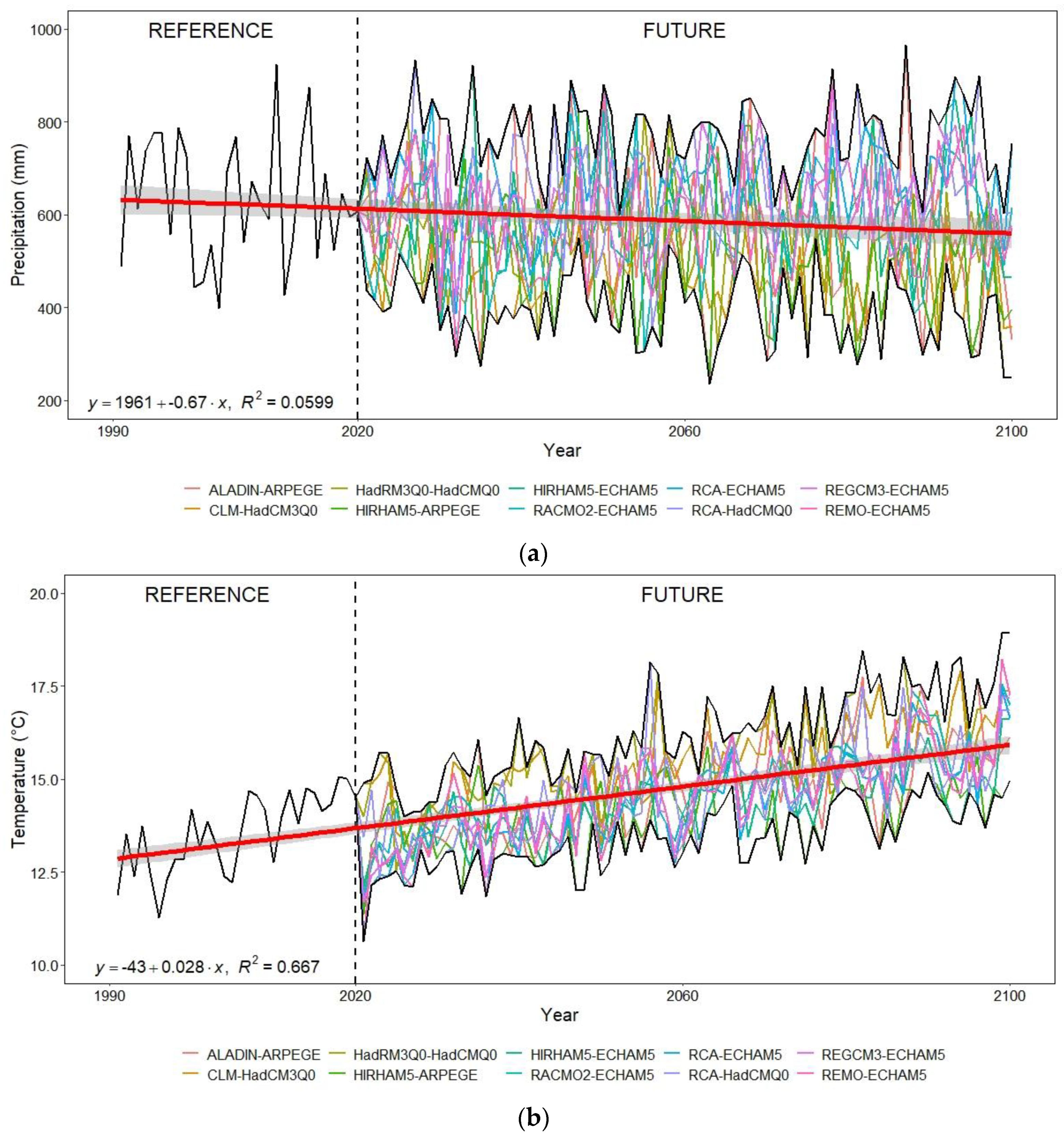
As a result of climate change, one of the most important factors affecting SWC is the amount of precipitation and its distribution over the years. The climate models project a slight decrease in the annual precipitation totals by the end of the century. The climate model runs show that the least amount of rain is expected by the CLM-HadCM3Q0 model (2021–2100) with approximately 471 mm/year on average and the largest precipitation was suggested by the RCA-ECHAM5 model in the 2021–2100 period with 674 mm/year. Compared to the amount of 634 mm/year in the reference period (1991–2020; Figure 2a), the former suggests a precipitation decrease (the largest among the 10 RCMs) while the latter suggests a slight increase. Based on all 10 climate models, it is expected that the total average annual precipitation will decrease to 582 mm/year by the end of the century.
Another important factor affecting SWC is the air temperature. There is a clear indication by the climate models that air temperatures will rise toward the end of the century (Figure 2b). All climate models show an increase in air temperature for both the minimum and maximum values. All 10 climate models estimated higher average air temperature by the end of the century than the reference period average annual mean temperature (13.57 °C). In general, the models show a 15.2% higher increase in the daily temperature minimums compared to the daily maximum value changes (7.30%; Figure 2b) by 2100. The red line in Figure 2b is a trendline for all 10 climate models, which shows a substantial temperature increase over the years.
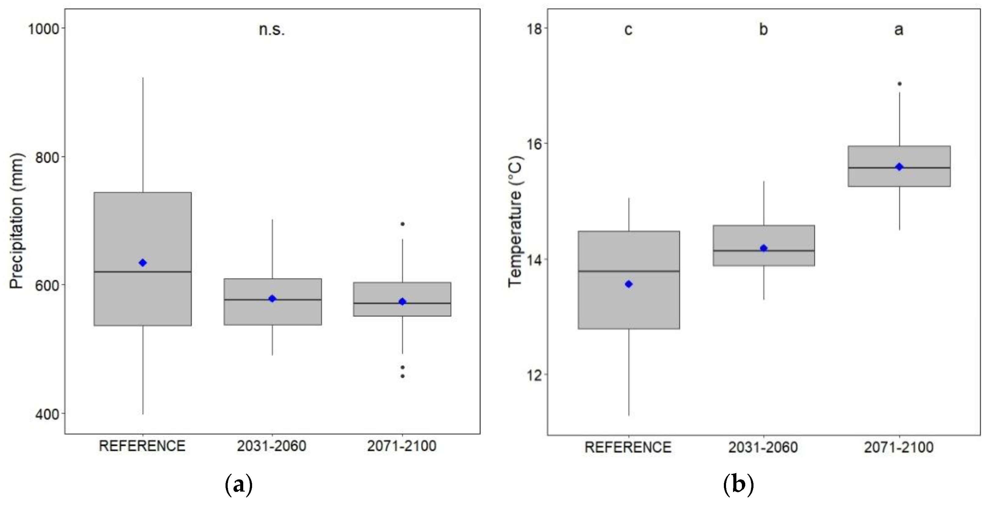
When we review the two future 30-year periods, a precipitation decrease is expected; however, the precipitation totals are not significantly different in the future scenarios compared to the reference period (Figure 3a). On the other hand, a significant increase in overall air temperature is expected by the climate models in the near future, which is projected to further increase on a significant level toward the end of the century (Figure 3b).
3.2. HYDRUS 1D Model Calibration and Validation
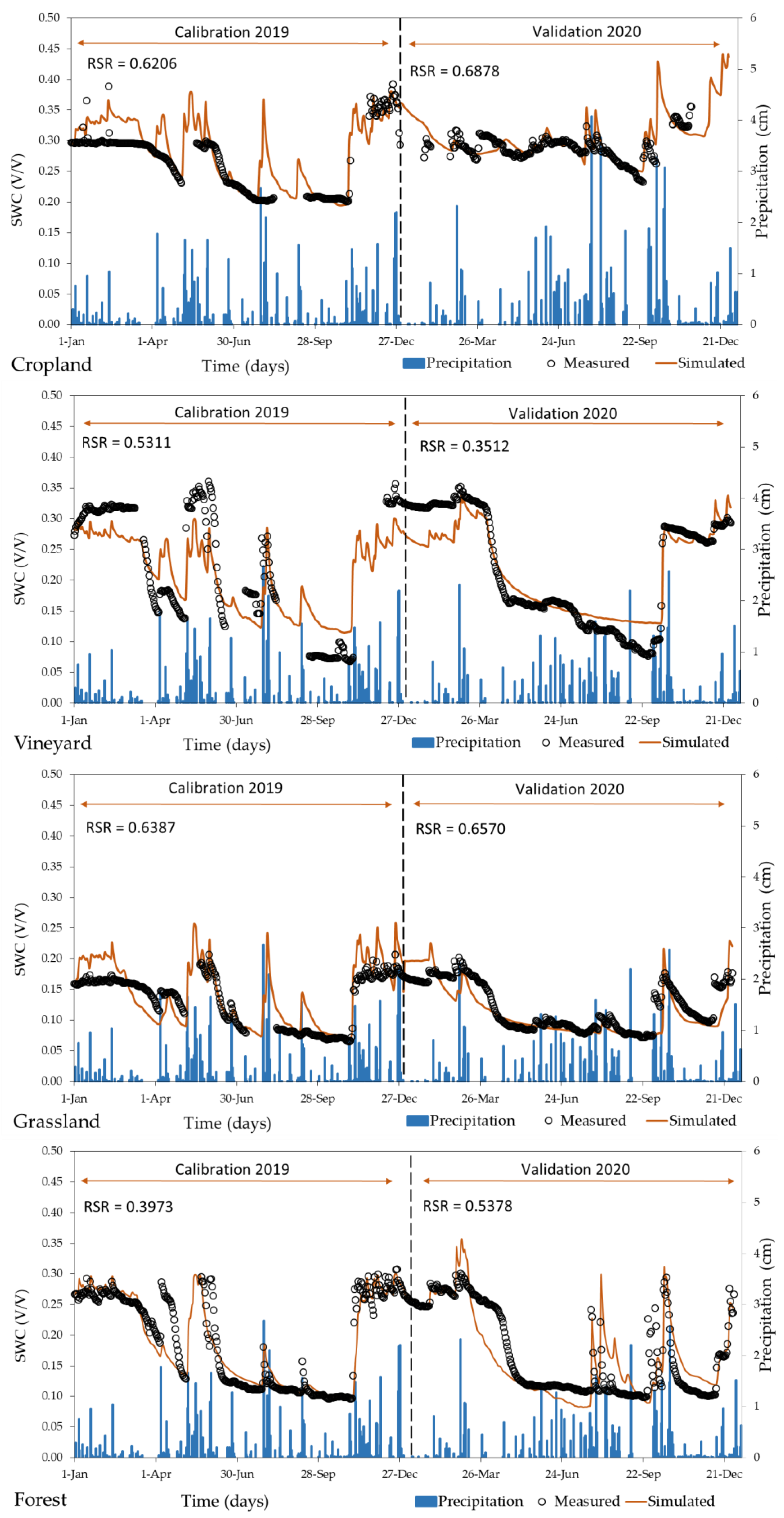
For all land use types, the model calibration (2019 SWC data) and validation (2020 SWC data) were based on the guidelines of RSR ≤ 0.70 suggested by Moriasi et al. [45,46]. The RSR values of the different model runs are shown in Figure 4.
In the validation period, for the vineyard site, the model underestimated SWC in the winter periods, while for the grassland, the model overestimated observed SWC. For both vineyard and grassland sites, the 2020 validation year showed very limited precipitation events during the summer, further reduced by surface runoffs on these sloping and strongly sloping sites. The model performance was the worst for the cropland site. The best model performance was observed for the forest SWCs, where the model nicely followed the resulting changes in SWCs from all recorded precipitation events (Figure 4).
3.3. Climate Change Impact on Extreme SWC Values
SWC is a sensitive parameter as plants can only tolerate and effectively utilize a certain range of water in the soil. Too much water can cause limitation in soil aeration, while a lack of sufficient moisture in the soil also causes stress for the plants. The total number of days per year below wilting point (WP) and above field capacity (FC) at 15 cm depth is summarized in Table 2. Grassland had the highest number of days outside optimal SWC values, with 289.8 day/year. The inland water and high water table levels caused 52.4 days/year above FC for the cropland, where no below WP days were noted. In contrast, the vineyard site is characterized by the most balanced soil–water regime, with most of the days (343.8 ± 27.5) falling within the optimal water content level (Table 2). Interestingly, all land use types are affected by too low SWC values when outside the optimal values, except for cropland, where the opposite trend of too wet days causes problems with SWC extending FC.
The near future scenarios resulted in mixed outcomes. For the grassland, only one climate model (HadRM3Q0-HadCMQ0) showed fewer dry days (SWC < WP) by 5.2%. For the forest soil, CLM-HadCM3Q0 and HIRHAM5-ARPEGE models showed increased numbers of critical SWCs, where up to a 66% increase in the days under WP might be expected. Among all investigated land use types, the vineyard had the lowest number of days outside optimal SWC conditions (6.2%). While some climate models are projecting smaller changes in the near-future SWC values, some climate models such as the CLM-HadCM3Q0 suggest the tripling of these days over the period of 2041–2050. Overall, climate change will likely negatively impact the more intensively managed land use types, i.e., the vineyard and cropland, where most of the models show a decrease (although not all significant) in the number of optimal SWC days for both future periods. However, the vineyard and cropland are to face opposite problems; the pattern is similar to the reference period: more dry days in the vineyard, and more too wet days in the cropland (Table 2).
Data suggested by RCM runs for the far future (2081–2090) also show mixed results on the number of days when SWCs are outside optimal ranges. Depending on the climate model used for the scenario analysis, the modeled values showed both decreases and increases in the SWC values for all land use types. A positive overall effect was projected only for the forest soil, with an average of 6.39% fewer days when SWCs are outside optimal conditions. In the longer term, the vineyard showed the highest vulnerability to climatic conditions, where the number of days with SWC under wilting point might triple. Among the five chosen climate models, only the RCA-ECHAM5 resulted in a positive outcome, which was expected as this model was selected as it projected the highest precipitation for future periods.
Data on SWCs based on the reference, near future, and far future model runs were analyzed on a monthly average SWC basis (data not shown). We found a clear trend showing the highest SWCs in the winter periods (December, January, and February) and the lowest in the late summer and early fall. Around March, a continuous SWC decrease begins and lasts until July–September, and the soil water begins to fill up the pore space again. For the vineyard and forest, the lowest SWCs were noted in September, and in August for the cropland. In the grassland site, the lowest SWC is reached earlier in the summer—by July, the SWC is already very low.
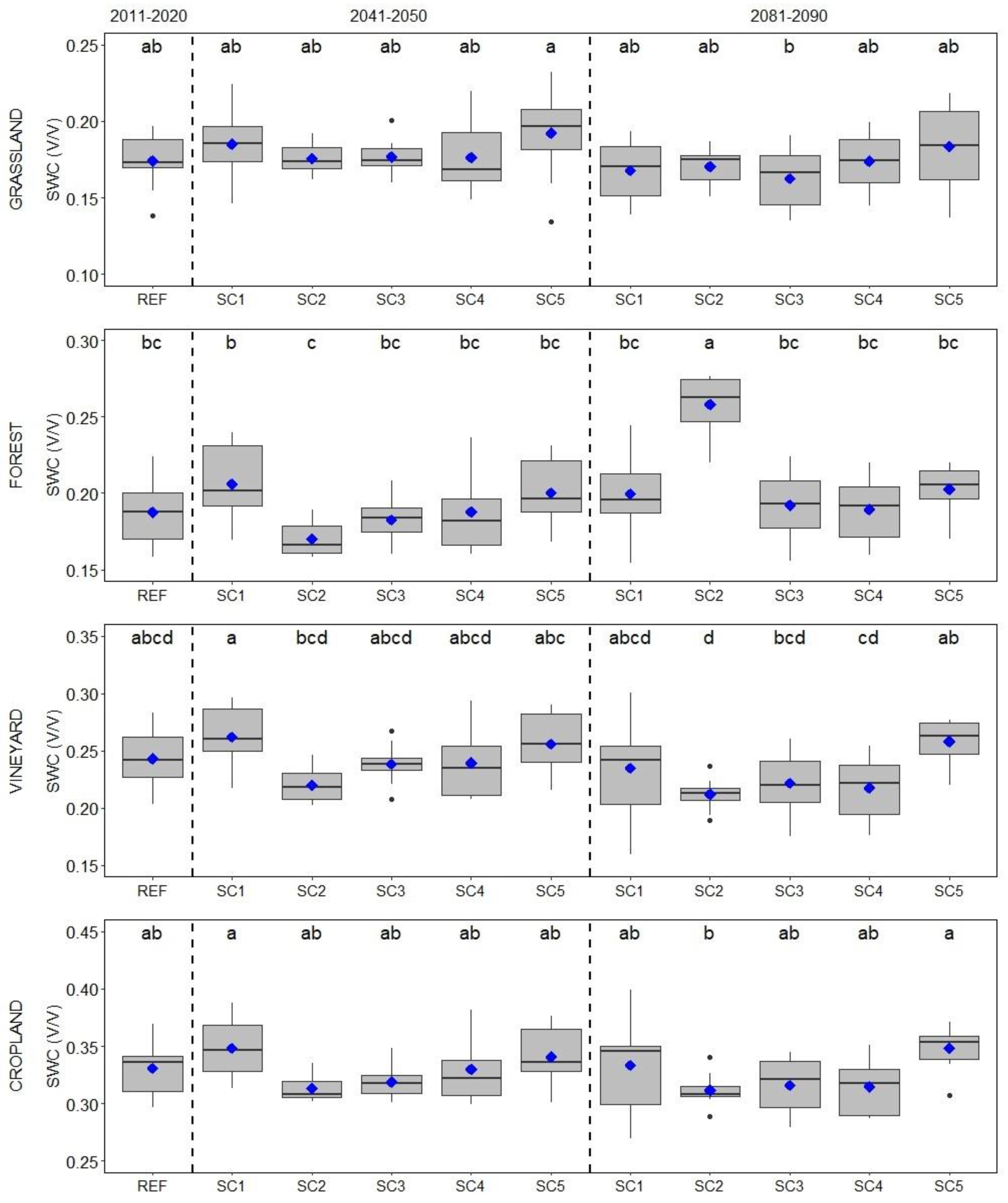
Statistical differences between the SWC values simulated for the different periods are shown in Figure 5. The grassland and cropland SWCs seem to be effected to a smaller degree in the future compared to the reference years, as the projected number of days outside of the optimal range is not significantly different. Similar results were estimated for the vineyard soil; while many scenarios have significantly higher or lower SWCs among projections, the reference data are still not significantly different from these prognoses. Only the far future scenario for forest soil showed significant differences from the reference SWCs, which is the above-mentioned CLM-HadCM3Q0 model (Figure 5).
4. Discussion
The results from various RCM runs showed consistently increasing temperatures over time, with a 1.8 °C higher average temperature toward the end of the century at our study sites. At the same time, precipitation amounts based on model averages are expected to be continuously decreasing. These factors affect soil water contents, and the agricultural lands need to be assessed to lessen any adverse effects arising from changing climatic conditions. At our research catchment, we observed a continuous decrease in yearly precipitation totals and an increase in air temperatures in recent years. Therefore, we aimed to outline future scenarios that might significantly change SWC in different land use types, influencing the directions of land use selection, future crop production, and agricultural land management practices.
The studied cropland is located at a low-lying part of the catchment, where the water table is shallow. This is clearly expressed by the measured SWCs reaching saturation levels after large rain events. While currently, the inland water might pose a great risk for the crops planted in this area, the decreasing overall precipitation and increasing air temperature could seemingly positively influence this phenomenon. However, the data from the near future climate models had some estimated increases in SWCs, as well (ALADIN-ARPEGE, HIRHAM5-ARPEGE, RCA-ECHAM5; Table 2). The HYDRUS 1D model showed for all RCM simulations that reaching field capacity is mostly occurring during the winter months, from December to February. The worst model performance for the cropland site can be due to tillage operations and crop rotation, which affect SWC time series; therefore, calibrating the model is more challenging, and we expected higher RSR values. Soil water changes in the cropland are highly dependent on the soil management system in addition to meteorological conditions. Soil tillage operation normally occurs up to 40 cm soil depth in the region, which might result in several soil physical changes affecting SWC. Some of the most important changes in soil properties caused by tillage include bulk density and water infiltration rate. Reduced soil bulk density followed by tillage operations can help water move deeper into the soil, consequently increasing water infiltration [14]. At our research site, moldboard plowing only happens every few years. Shallow plowing and seedbed preparation management practices are performed more often on the cropland, affecting the top 10–20 cm of the soil by disrupting its soil physical properties and, consequently, soil hydrological properties. Besides causing temporal changes in soil physical properties, which cannot be considered in the model setup, these operations influence measurement uncertainty, as well. This feature results in the lower model performance for the cropland. In winter, when the topsoil and the water in it can be frozen, the sensors may not measure SWC properly. For example, in the winter of 2019, sensors in the cropland recorded 4–5 sudden increases. These could have been caused by soil thawing, and the sensors measured the total water content.
The type of vegetation being planted at the cropland site influences the water usage and deficiency, and evapotranspiration rates. In our calibration and validation period, we had winter wheat and maize in 2019 and 2020, respectively. In the crop rotation in our study area, winter wheat or triticale is sown in the fall and harvested in the summer, and maize or sunflower is sown in the spring and harvested in the fall. The main plant-related differences between winter and summer crops are the length, structure, and density of the below-ground biomass and root system, and the above-ground plant canopy structure or leaf area index. These plant traits can greatly influence soil moisture, water uptake by plants [47], and the overall evapotranspiration process [48]. Another main difference between the two types of crops is the sowing row distances, which can be three times higher for maize compared to triticale [49]. However, after approximately five or six years, the crop rotation might have the full circle, and the data gathered for SWC can be used for each general crop type.
Our results indicate that vineyards are the most vulnerable land use types to projected climate change at the study catchment. Most of our HYDRUS 1D model results considering far-future RCM runs indicate over triple the number of days below wilting point than for the past decade (2011–2020). Most of the RCM simulations showed that September is the driest month out of the year for vineyards, and SWCs decline from February. These extreme drying conditions in the vineyards in 2020 (Figure 4) might be due to the sloping conditions resulting in high runoff generation during larger precipitation events before the rainwater enters deeper into the soil layer. The study catchment and its surrounding area have a long history of viticulture [50], and its high quality should be maintained. Severe heat stress can result in significantly declining grapevine productivity mainly due to the limitations in photosynthesis and damaged physiological traits [51]. Above the upper limit of the optimal air temperature range (35 °C [52]), the grapevine growth and fruit production can decline and the quality of wine might be further affected. While during the referenced decade, on average, 4.4 days per year were higher than the 35 °C maximum air temperature, the climate models in the present study projected this number to increase almost threefold, averaging 11.1 days per year above the optimal temperature for the far future scenarios. These data show that the agricultural sector needs to be prepared, and many current water retention measures taken to mitigate the negative effects should be widely implemented. For example, the adaptation of no-till practices can increase water table levels, as it was highlighted by Eeswaran et al. [29], who found that the water table can rise by 0.1 to 0.5 m on a watershed scale. No-till can also lower soil temperature while increasing SWC [53]. While overall annual precipitation totals might be similar in the present and near future, the rainfall patterns could differ. Individual rain events with short intervals between the events can be more beneficial for SWC and ecosystem processes than longer intervals [54].
The grassland at the research site has the lowest SWC overall among all land use types. We also noticed that many of the plants at the site are already drought-tolerant species such as Helianthemum nummularium, Salvia pratensis, or Thymus sp. [55,56]. While most days of the year, the SWCs are below the wilting point in this site at 15 cm depth, the shallow-rooted and drought-tolerant plants can still thrive. Although an increase in air temperature and consequently higher evaporation rates are expected, the different RCM simulations do not project significant changes in the SWCs or the number of days below WP to considerably increase at the grassland. Under warming environmental conditions, increased evapotranspiration might reduce soil water availability below a stress threshold, leading to the suppression of plant growth and root and microbial activities in grassland ecosystems [57]. Our soil hydrological model simulates very low SWCs from April to October for all RCM models in the grassland. Therefore, without additional water retention measures at this site, the drought-tolerant plant species will dominate in the near future.
The results based on different RCM outputs showed mixed outcomes on forest SWCs. Some model runs indicated positive outcomes, as the number of days when the SWCs were within the optimal range showed an increase. However, some models showed a decrease, although these changes were not statistically significant. Similar to the vineyard data, the driest months for the SWC are August and September for the forest, and therefore have the highest potential for drought conditions. Forest soil temperatures are less likely to fluctuate as much as the other land use types where direct contact of the sunlight with the soil is more likely. At the study site, forest soils’ temperature at 15 cm depth was approximately 1.5 °C lower compared to the other sites during the past years, which might make this site’s SWC less affected by climatic variations than the other investigated sites. However, it has been noted that forest ecosystems in this region are particularly vulnerable to climate change [21]. Baldrian et al. [58] found that increases in SWC resulted in increased microbial biomass in forests, where litter decomposition has a vital role in forest ecosystems. Therefore, the predicted reduction in SWC might decrease microbial enzyme activities, further affecting soil health. Forests have high risks of other climate change-related negative impacts, such as forest diseases resulting in tree mortality or higher susceptibility to pathogens [59].
As an outlook, implementing soil water retention measurements might be helpful in the investigated lands. Organic matter content in soils can greatly affect soil water retention, and restoring organic matter in degraded soils might increase plant-available water capacity [60], and therefore might be a tool to help mitigate climate change-related SWC deficits. Croplands and vineyards receive additional fertilizer more frequently than forest or grasslands to achieve higher crop and fruit yields. In the study areas, this is normally carried out every few years. Organic fertilizer (mainly horse or cow manure) is often applied, especially in vineyards, consequently increasing organic matter content and soil moisture retention of the soils, as organic manure can help retain water in the upper 100 cm of the soils and can be used to enhance crop yield, water use efficiency, and soil aggregate stability [61,62]. This is necessary in the study catchment, as both sites have significantly lower SOC present compared to the forest or grassland soils.
5. Conclusions
In the present study, we adopted a hydrology model combined with future climate data synthesized into five models representing near and far future scenarios to simulate soil water content changes. Our results indicate potentially extensive changes in SWCs for all investigated land use types. Future climate change showed possible negative effects on the vineyard and cropland soils, while similar to current soil water content is expected for the grassland and forest soils. The most accelerated soil drying can be expected in the vineyard or the steepest slopes of the catchment. Therefore, we conclude that soil moisture retention measures should be implemented and applied in the near future, especially for areas with high degrees of surface runoff. Such measures might include terraces for grapevines, which are not yet common in the catchment, or the implementation of conservational or no-till soil management practices. These measures need to be carefully assessed and applied if there is potential to mitigate the negative impacts of climate change and to preserve the sustainability of current land use types for future use in this area.
This study is the first analysis for the area of concern, and the modeling methodology can be further refined. For example, we plan to extend the study to also consider new RCP-based scenarios. The current modeling only considers maize in future model runs. Including more details in the description of cropland management (e.g., crop rotation, tillage, fertilizer, and irrigation) is also a necessary step to develop a more general picture of adaptation strategies.
Author Contributions
Conceptualization, G.G., Z.B. and Á.H.; methodology, Á.H., A.K. and G.G.; validation, C.F.; formal analysis, T.Z.; resources, C.F., E.T., A.K. and Á.H.; data curation, Á.H. and Z.B.; writing—original draft preparation, G.G., Z.B., C.F. and Á.H.; writing—review and editing, Z.B., G.G. and E.T.; visualization, T.Z. and Á.H.; supervision, Á.H.; project administration, Á.H.; funding acquisition, Á.H. All authors have read and agreed to the published version of the manuscript.
Funding
This material is based on work supported by the Hungarian National Research Fund (OTKA/NKFI) project OTKA FK-131792. A.K. was supported by the János Bolyai Research Scholarship of the Hungarian Academy of Sciences (grant no. BO/00254/20/10) and by the grant “Advanced research supporting the forestry and wood-processing sector’s adaptation to global change and the 4th industrial revolution”, no. CZ.02.1.01/0.0/0.0/16_019/0000803, financed by OP RDE. The APC was funded by A.H. and Z.B.
Institutional Review Board Statement
Not applicable.
Informed Consent Statement
Not applicable.
Data Availability Statement
Not applicable.
Acknowledgments
The authors would like to thank Imre Zagyva, Szandra Baklanov, and Imre Potyó for their help with field instrumentation.
Conflicts of Interest
The authors declare no conflict of interest.
References
- Easterling, D.; Meehl, G.; Parmesan, C.; Changnon, S.; Karl, T.; Mearns, L. Climate extremes: Observations, modeling, and impacts. Science 2000, 289, 2068–2074. [Google Scholar] [CrossRef] [PubMed] [Green Version]
- Scheifinger, H.; Menzel, A.; Koch, E.; Peter, C. Trends of spring time frost events and phenological dates in Central Europe. Theor. Appl. 2003, 74, 41–51. [Google Scholar] [CrossRef]
- Lavalle, C.; Micale, F.; Houston, T.D.; Camia, A.; Hiederer, R.; Lazar, C.; Conte, C.; Amatulli, G.; Genovese, G. Climate change in Europe. 3. Impact on agriculture and forestry. A review. Agron. Sustain. Dev. 2009, 29, 433–446. [Google Scholar] [CrossRef] [Green Version]
- Arora, N.K. Impact of climate change on agriculture production and its sustainable solutions. Environ. Sustain. 2019, 2, 95–96. [Google Scholar] [CrossRef] [Green Version]
- IPCC. Climate Change 2022, Impacts, Adaptation and Vulnerability. WGII Sixth Assessment Report. Available online: https://www.ipcc.ch/report/ar6/wg2/ (accessed on 19 March 2022).
- Ragab, R.; Prudhomme, C. SW—Soil and water: Climate change and water resources management in arid and semi-arid regions: Prospective and challenges for the 21st Century. Biosyst. Eng. 2002, 81, 3–34. [Google Scholar] [CrossRef]
- Ankenbauer, K.J.; Loheide Ii, S.P. The effects of soil organic matter on soil water retention and plant water use in a meadow of the Sierra Nevada, CA. Hydrol. Processes 2017, 31, 891–901. [Google Scholar] [CrossRef]
- Hudson, B.D. Soil organic matter and available water capacity. J. Soil Water Conserv. 1994, 49, 189. [Google Scholar]
- Kirkham, M.B. Chapter 10—Field Capacity, Wilting Point, Available Water, and the Nonlimiting Water Range. In Principles of Soil and Plant Water Relations, Second Edition; Kirkham, M.B., Ed.; Academic Press: Boston, MA, USA, 2014; pp. 153–170. [Google Scholar] [CrossRef]
- Abdelkadir, A.; Yimer, F. Soil water property variations in three adjacent land use types in the Rift Valley area of Ethiopia. J. Arid Environ. 2011, 75, 1067–1071. [Google Scholar] [CrossRef]
- Hota, S.; Mishra, V.; Mourya, K.K.; Giri, K.; Kumar, D.; Jha, P.K.; Saikia, U.S.; Prasad, P.V.V.; Ray, S.K. Land use, landform, and soil management as determinants of soil physicochemical properties and microbial abundance of Lower Brahmaputra Valley, India. Sustainability 2022, 14, 2241. [Google Scholar] [CrossRef]
- Jakab, G.; Németh, T.; Csepinszky, B.; Madarász, B.; Szalai, Z.; Kertész, Á. The influence of short term soil sealing and crusting on hydrology and erosion at Balaton Uplands, Hungary. Carpathian J. Earth Environ. Sci. 2013, 8, 147–155. [Google Scholar]
- Saeidi, S.; Grósz, J.; Sebők, A.; Barros, V.D.d.; Waltner, I. Analysis results of land-use and land cover changes of Szilas catchment from 1990. Tájökológiai Lapok 2019, 17, 265–275. [Google Scholar]
- Blanco-Canqui, H.; Wienhold, B.J.; Jin, V.L.; Schmer, M.R.; Kibet, L.C. Long-term tillage impact on soil hydraulic properties. Soil Tillage Res. 2017, 170, 38–42. [Google Scholar] [CrossRef] [Green Version]
- Jakab, G.; Madarász, B.; Szabó, J.; Tóth, A.; Zacháry, D.; Szalai, Z.; Kertész, Á.; Dyson, J. Infiltration and soil loss changes during the growing season under ploughing and conservation tillage. Sustainability 2017, 9, 1726. [Google Scholar] [CrossRef] [Green Version]
- Rieder, Á.; Madarász, B.; Szabó, J.A.; Zacháry, D.; Vancsik, A.; Ringer, M.; Szalai, Z.; Jakab, G. Soil organic matter alteration velocity due to land-use change: A case study under conservation agriculture. Sustainability 2018, 10, 943. [Google Scholar] [CrossRef] [Green Version]
- van Noordwijk, M.; Lawson, G.; Hairiah, K.; Wilson, J. Root distribution of trees and crops: Competition and/or complementarity. In Tree-Crop Interactions: Agroforestry in a Changing Climate, 2nd ed.; Ong, C.K., Black, C.R., Wilson, J., Eds.; NORA: Wallingford, UK, 2015. [Google Scholar]
- Bloodworth, M.E.; Burleson, C.A.; Cowley, W.R. Root distribution of some irrigated crops using undisrupted soil cores. Agron. J. 1958, 50, 317–320. [Google Scholar] [CrossRef]
- Hajdu, E. Viticulture of Hungary. Acta Agrar. Debr. 2018, 150, 175–182. [Google Scholar] [CrossRef]
- Nicolescu, V.-N.; Rédei, K.; Mason, W.L.; Vor, T.; Pöetzelsberger, E.; Bastien, J.-C.; Brus, R.; Benčať, T.; Đodan, M.; Cvjetkovic, B.; et al. Ecology, growth and management of black locust (Robinia pseudoacacia L.), a non-native species integrated into European forests. J. For. Res. 2020, 31, 1081–1101. [Google Scholar] [CrossRef] [Green Version]
- Farkas, C.; Gelybó, G.; Bakacsi, Z.; Horel, Á.; Hagyó, A.; Dobor, L.; Kása, I.; Tóth, E. Impact of expected climate change on soil water regime under different vegetation conditions. Biologia 2014, 69, 1510–1519. [Google Scholar] [CrossRef]
- Wang, X.; Li, Y.; Chen, X.; Wang, H.; Li, L.; Yao, N.; Liu, D.L.; Biswas, A.; Sun, S. Projection of the climate change effects on soil water dynamics of summer maize grown in water repellent soils using APSIM and HYDRUS-1D models. Comput. Electron. Agric. 2021, 185, 106142. [Google Scholar] [CrossRef]
- Xiao, D.; Liu, D.L.; Wang, B.; Feng, P.; Bai, H.; Tang, J. Climate change impact on yields and water use of wheat and maize in the North China Plain under future climate change scenarios. Agric. Water Manag. 2020, 238, 106238. [Google Scholar] [CrossRef]
- Qian, S.; Fu, Y.; Pan, F. Climate change tendency and grassland vegetation response during the growth season in Three-River Source Region. Sci. China Earth Sci. 2010, 53, 1506–1512. [Google Scholar] [CrossRef]
- Autovino, D.; Rallo, G.; Provenzano, G. Predicting soil and plant water status dynamic in olive orchards under different irrigation systems with Hydrus-2D: Model performance and scenario analysis. Agric. Water Manag. 2018, 203, 225–235. [Google Scholar] [CrossRef]
- Horel, Á.; Tóth, E.; Gelybó, G.; Dencső, M.; Farkas, C. Biochar amendment affects soil water and CO2 regime during Capsicum annuum plant growth. Agronomy 2019, 9, 58. [Google Scholar] [CrossRef] [Green Version]
- Sheikh Goodarzi, M.; Jabbarian Amiri, B.; Azarnivand, H.; Waltner, I. Watershed hydrological modelling in data scarce regions; integrating ecohydrology and regionalization for the southern Caspian Sea basin, Iran. Heliyon 2021, 7, e06833. [Google Scholar] [CrossRef]
- DeJonge, K.C.; Ascough, J.C.; Andales, A.A.; Hansen, N.C.; Garcia, L.A.; Arabi, M. Improving evapotranspiration simulations in the CERES-Maize model under limited irrigation. Agric. Water Manag. 2012, 115, 92–103. [Google Scholar] [CrossRef] [Green Version]
- Eeswaran, R.; Nejadhashemi, A.P.; Kpodo, J.; Curtis, Z.K.; Adhikari, U.; Liao, H.; Li, S.-G.; Hernandez-Suarez, J.S.; Alves, F.C.; Raschke, A.; et al. Quantification of resilience metrics as affected by conservation agriculture at a watershed scale. Agric. Ecosyst. Environ. 2021, 320, 107612. [Google Scholar] [CrossRef]
- Dövényi, Z. Magyarország Kistájainak Katasztere; MTA Földrajztudományi Kutatóintézet: Budapest, Hungary, 2010; 876p. (In Hungarian) [Google Scholar]
- IUSS Working Group Wrb. World reference base for soil resources 2014, updated 2015. In World Soil Resources Reports No. 106; FAO: Rome, Italy, 2015. [Google Scholar]
- Cresswell, H.P.; Green, T.W.; McKenzie, N.J. The adequacy of pressure plate apparatus for determining soil water retention. Soil Sci. Soc. Am. J. 2008, 72, 41–49. [Google Scholar] [CrossRef]
- Simunek, J.; Sejna, M.; van Genuchten, M.T. The HYDRUS Software Package for Simulating the Two-and Three-Dimensional Movement of Water, Heat, and Multiple Solutes in Variably-Saturated Media; PC-Progress: Prague, Czech Republic, 2007. [Google Scholar]
- Pachepsky, Y.; Timlin, D.; Rawls, W. Generalized Richards’ equation to simulate water transport in unsaturated soils. J. Hydrol. 2003, 272, 3–13. [Google Scholar] [CrossRef]
- van Genuchten, M.T. A closed-form equation for predicting the hydraulic conductivity of unsaturated soils. Soil Sci. Soc. Am. J. 1980, 44, 892–898. [Google Scholar] [CrossRef] [Green Version]
- van Genuchten, M.; Leij, F.; Yates, S. The RETC Code for Quantifying the Hydraulic Functions of Unsaturated Soils; USA Salinity Laboratory, USDA, ARS: Riverside, CA, USA, 1991.
- Feddes, R.A.; Hoff, H.; Bruen, M.; Dawson, T.; DeRosnay, P.; Dirmeyer, P.; Jackson, R.B.; Kabat, P.; Kleidon, A.; Lilly, A.; et al. Modeling root water uptake in hydrological and climate models. Bull. Am. Meteorol. Soc. 2001, 82, 2797–2809. [Google Scholar] [CrossRef] [Green Version]
- Wesseling, J.G.; Elbers, J.A.; Kabat, P.; van den Broek, B.J. SWATRE: Instructions for Input; Winand Staring Centre: Wageningen, The Netherlands, 1991. [Google Scholar]
- Hargreaves, G.H.; Samani, Z.A. Reference crop evapotranspiration from temperature. Appl. Eng. Agric. 1985, 1, 96–99. [Google Scholar] [CrossRef]
- Cornes, R.C.; van der Schrier, G.; van den Besselaar, E.J.M.; Jones, P.D. An Ensemble Version of the E-OBS Temperature and Precipitation Data Sets. J. Geophys. Res. Atmos. 2018, 123, 9391–9409. [Google Scholar] [CrossRef] [Green Version]
- Dobor, L.; Barcza, Z.; Hlásny, T.; Havasi, Á.; Horváth, F.; Ittzés, P.; Bartholy, J. Bridging the gap between climate models and impact studies: The FORESEE Database. Geosci. Data J. 2015, 2, 1–11. [Google Scholar] [CrossRef] [PubMed]
- Kern, A.; Dobor, L.; Horváth, F.; Hollós, R.; Márta, G.; Barcza, Z. FORESEE: Egy publikus meteorológiai adatbázis a Kárpát-medence tágabb térségére (extended abstract). Az elmélet és a gyakorlat találkozása a térinformatikában. In Proceedings of the X. Térinformatikai Konferencia és Szakkiállítás, Debrecen, Hungary, 23–24 May 2019; pp. 131–138. [Google Scholar]
- Ines, A.V.M.; Hansen, J.W. Bias correction of daily GCM rainfall for crop simulation studies. Agric. For. Meteorol. 2006, 138, 44–53. [Google Scholar] [CrossRef] [Green Version]
- Thornton, P.E.; Hasenauer, H.; White, M.A. Simultaneous estimation of daily solar radiation and humidity from observed temperature and precipitation: An application over complex terrain in Austria. Agric. For. 2000, 104, 255–271. [Google Scholar] [CrossRef]
- Moriasi, D.N.; Arnold, J.G.; Van Liew, M.W.; Bingner, R.L.; Harmel, R.D.; Veith, T.L. Model evaluation guidelines for systematic quantification of accuracy in watershed simulations. Trans. ASABE 2007, 50, 885–900. [Google Scholar] [CrossRef]
- Moriasi, N.D.; Gitau, W.M.; Pai, N.; Daggupati, P. Hydrologic and water quality models: Performance measures and evaluation criteria. Trans. ASABE 2015, 58, 1763–1785. [Google Scholar] [CrossRef] [Green Version]
- Hupet, F.; Lambot, S.; Feddes, R.A.; van Dam, J.C.; Vanclooster, M. Estimation of root water uptake parameters by inverse modeling with soil water content data. Water Resour. Res. 2003, 39, 1–16. [Google Scholar] [CrossRef] [Green Version]
- Gardner, W.R.; Ehlig, C.F. The influence of soil water on transpiration by plants. J. Geophys. Res. 1963, 68, 5719–5724. [Google Scholar] [CrossRef]
- Nielsen, D.C.; Miceli-Garcia, J.J.; Lyon, D.J. Canopy cover and leaf area index relationships for wheat, triticale, and corn. Agron. J. 2012, 104, 1569–1573. [Google Scholar] [CrossRef] [Green Version]
- Varga, P.; Májer, J. The use of organic wastes for soil-covering of vineyards. ISHS Acta Hortic. 2004, 652, 191–197. [Google Scholar] [CrossRef]
- Gutiérrez-Gamboa, G.; Zheng, W.; Martínez de Toda, F. Strategies in vineyard establishment to face global warming in viticulture: A mini review. J. Sci. Food Agric. 2021, 101, 1261–1269. [Google Scholar] [CrossRef] [PubMed]
- Hochberg, U.; Batushansky, A.; Degu, A.; Rachmilevitch, S.; Fait, A. Metabolic and physiological responses of Shiraz and Cabernet Sauvignon (Vitis vinifera L.) to near optimal temperatures of 25 and 35 °C. Int. J. Mol. Sci. 2015, 16, 24276–24294. [Google Scholar] [CrossRef] [PubMed] [Green Version]
- Gelybó, G.; Barcza, Z.; Dencső, M.; Potyó, I.; Kása, I.; Horel, Á.; Pokovai, K.; Birkás, M.; Kern, A.; Hollós, R.; et al. Effect of tillage and crop type on soil respiration in a long-term field experiment on chernozem soil under temperate climate. Soil Tillage Res. 2022, 216, 105239. [Google Scholar] [CrossRef]
- Fay, P.A.; Kaufman, D.M.; Nippert, J.B.; Carlisle, J.D.; Harper, C.W. Changes in grassland ecosystem function due to extreme rainfall events: Implications for responses to climate change. Glob. Change Biol. 2008, 14, 1600–1608. [Google Scholar] [CrossRef]
- Fridley, J.D.; Grime, J.P.; Askew, A.P.; Moser, B.; Stevens, C.J. Soil heterogeneity buffers community response to climate change in species-rich grassland. Glob. Change Biol. 2011, 17, 2002–2011. [Google Scholar] [CrossRef]
- Grime, J.P.; Fridley, J.D.; Askew, A.P.; Thompson, K.; Hodgson, J.G.; Bennett, C.R. Long-term resistance to simulated climate change in an infertile grassland. Proc. Natl. Acad. Sci. USA 2008, 105, 10028. [Google Scholar] [CrossRef] [PubMed] [Green Version]
- Liu, W.; Zhang, Z.H.E.; Wan, S. Predominant role of water in regulating soil and microbial respiration and their responses to climate change in a semiarid grassland. Glob. Change Biol. 2009, 15, 184–195. [Google Scholar] [CrossRef]
- Baldrian, P.; Šnajdr, J.; Merhautová, V.; Dobiášová, P.; Cajthaml, T.; Valášková, V. Responses of the extracellular enzyme activities in hardwood forest to soil temperature and seasonality and the potential effects of climate change. Soil Biol. Biochem. 2013, 56, 60–68. [Google Scholar] [CrossRef]
- Sturrock, R.N.; Frankel, S.J.; Brown, A.V.; Hennon, P.E.; Kliejunas, J.T.; Lewis, K.J.; Worrall, J.J.; Woods, A.J. Climate change and forest diseases. Plant Pathol. 2011, 60, 133–149. [Google Scholar] [CrossRef]
- Lal, R. Soil organic matter and water retention. Agron. J. 2020, 112, 3265–3277. [Google Scholar] [CrossRef]
- Liu, C.-A.; Li, F.-R.; Zhou, L.-M.; Zhang, R.-H.; Yu, J.; Lin, S.-L.; Wang, L.-J.; Siddique, K.H.M.; Li, F.-M. Effect of organic manure and fertilizer on soil water and crop yields in newly-built terraces with loess soils in a semi-arid environment. Agric. Water Manag. 2013, 117, 123–132. [Google Scholar] [CrossRef]
- He, Y.; Xu, C.; Gu, F.; Wang, Y.; Chen, J. Soil aggregate stability improves greatly in response to soil water dynamics under natural rains in long-term organic fertilization. Soil Tillage Res. 2018, 184, 281–290. [Google Scholar] [CrossRef]
Figure 1.
Area of the Csorsza study catchment showing locations of soil moisture and temperature sensors, rain gauges, and the main meteorological station.
Figure 1.
Area of the Csorsza study catchment showing locations of soil moisture and temperature sensors, rain gauges, and the main meteorological station.

Figure 2.
Expected (a) total annual precipitation amounts (mm) and (b) mean annual temperature values (°C) in the next 80 years, based on the different RCM simulations. Black lines represent the maximum and minimum values foreseen by the climate models, while the red line is the trendline for the models’ average.

Figure 3.
Projected (a) precipitation (mm) and (b) temperature (°C) change in the near (2031–2060) and far (2071–2100) future as compared to the reference years based on the 10 RCM simulations. The blue diamond indicates the means of the precipitation or temperature for the period. Different letters indicate statistically significant differences, while n.s. represents no significant differences among reference periods (one-way ANOVA and Tukey’s HSD test).

Figure 4.
Measured and simulated soil water contents (VWC) for the different land uses at 15 cm depths, indicating the calibration (2019) and validation (2020) periods.
Figure 4.
Measured and simulated soil water contents (VWC) for the different land uses at 15 cm depths, indicating the calibration (2019) and validation (2020) periods.

Figure 5.
Statistical data of the soil water contents from reference (2011–2020), the near future (2041–2050), and far future (2081–2090) model runs. The following abbreviations are used for the climate scenarios: REF, reference; SC1, ALADIN-ARPEGE; SC2, CLM-HadCM3Q0; SC3, HadRM3Q0-HadCMQ0; SC4, HIRHAM5-ARPEGE; SC5, RCA-ECHAM5. Data represent SWCs at 15 cm below the soil surface. The blue diamonds indicate the mean SWC of the given climate model run. Different letters indicate significant differences among average SWCs projected by the different model runs for each land use type (Tukey’s HSD test).


Table 1.
Soil characteristics of the land use types at 15 cm. θsat and θres represent the saturated and residual water content of the investigated soils, respectively. Different letters indicate significant differences among land use types per soil physical parameter (Wilcoxon test). SOC represents the soil organic carbon percent. N = 3 per land use types; ±SD.
| Land Use Types | Vineyard | Grassland | Forest | Cropland | |
|---|---|---|---|---|---|
| Soil Texture | Clay | Clay Loam | Silty Clay Loam | Silty Clay | |
| Bulk Density | g/cm3 | 1.23 ± 0.0 b | 1.33 ± 0.1 ab | 1.40 ± 0.1 a | 1.28 ± 0.17 ab |
| Sand | % | 12.1 ± 1.3 c | 22.7 ± 0.8 a | 15.9 ± 0.3 b | 10.4 ± 0.8 c |
| Silt | % | 36.2 ± 2.7 c | 39.9 ± 2.8 c | 54.9 ± 0.5 a | 44.8 ± 1.0 b |
| Clay | % | 51.8 ± 2.7 a | 37.5 ± 2.3 c | 29.2 ± 0.3 d | 44.8 ± 0.3 b |
| θsat | % | 57.1 ± 0.6 a | 51.8 ± 2.8 b | 46.4 ± 2.9 c | 54.6 ± 3.3 ab |
| θres | % | 4.6 ± 0.7 a | 4.4 ± 0.3 a | 2.6 ± 0.1 c | 3.2 ± 0.3 b |
| SOC | % | 1.93 ± 0.08 b | 3.81 ± 0.61 a | 5.34 ± 0.73 a | 1.70 ± 0.12 c |
| pH | - | 7.93 ± 0.10 b | 6.46 ± 0.10 c | 5.98 ± 0.14 c | 7.86 ± 0.12 a |
Table 2.
Expected number of days per year below wilting point (WP) or above field capacity (FC) at 15 cm below soil surface. Optimal represents the number of days between WP and FC. Data were retrieved based on reference data of 2011–2020 and near future (2041–2050) and far future (2081–2090) scenarios.
| Grassland | Vineyard | ||||||
| Years | Scenarios | <WP | Optimal | >FC | <WP | Optimal | >FC |
| 2011–2020 | REFERENCE | 289.8 ± 30.5 | 75.3 ± 30.3 | 0 ± 0 | 21.3 ± 27.4 | 343.8 ± 27.5 | 0 ± 0 |
| 2041–2050 | ALADIN-ARPEGE | 272.0 ± 44.9 | 93.1 ± 44.9 | 0 ± 0 | 19.4 ± 32.4 | 345.7 ± 32.5 | 0 ± 0 |
| CLM-HadCM3Q0 | 289.5 ± 27.5 | 75.6 ± 27.5 | 0 ± 0 | 77.3 ± 48.7 | 287.8 ± 48.5 | 0 ± 0 | |
| HadRM3Q0-HadCMQ0 | 292.8 ± 31.3 | 72.3 ± 31.3 | 0 ± 0 | 28.9 ± 38.9 | 336.2 ± 38.9 | 0 ± 0 | |
| HIRHAM5-ARPEGE | 273.9 ± 44.4 | 91.2 ± 44.3 | 0 ± 0 | 56.6 ± 47.5 | 308.5 ± 47.4 | 0 ± 0 | |
| RCA-ECHAM5 | 241.4 ± 54.3 | 123.7 ± 54.1 | 0 ± 0 | 16.2 ± 23.2 | 348.9 ± 23.1 | 0 ± 0 | |
| 2081–2090 | ALADIN-ARPEGE | 297.2 ± 39.2 | 67.9 ±3 9.1 | 0 ± 0 | 77.1 ± 74.7 | 288.0 ± 74.6 | 0 ± 0 |
| CLM-HadCM3Q0 | 286.9 ± 28.0 | 78.2 ±2 7.8 | 0 ± 0 | 99.0 ± 41.9 | 266.1 ± 42.0 | 0 ± 0 | |
| HadRM3Q0-HadCMQ0 | 298.7 ± 38.4 | 66.4 ± 38.2 | 0 ± 0 | 76.1 ± 59.0 | 289.0 ± 58.9 | 0 ± 0 | |
| HIRHAM5-ARPEGE | 279.9 ± 43.2 | 85.2 ± 43.1 | 0 ± 0 | 89.9 ± 64.5 | 275.2 ± 64.3 | 0 ± 0 | |
| RCA-ECHAM5 | 256.5 ± 48.6 | 108.6 ± 48.6 | 0 ± 0 | 20.4 ± 31.9 | 344.7 ± 32.0 | 0 ± 0 | |
| Forest | Cropland | ||||||
| Years | Scenarios | <WP | Optimal | >FC | <WP | Optimal | >FC |
| 2011–2020 | REFERENCE | 99.7 ± 61.6 | 265.4 ± 61.5 | 0 ± 0 | 0 ± 0 | 312.7 ± 48.2 | 52.4 ± 48.1 |
| 2041–2050 | ALADIN-ARPEGE | 51.7 ± 55.1 | 313.4 ± 55.2 | 0 ± 0 | 0 ± 0 | 288.4 ± 63.5 | 76.7 ± 63.5 |
| CLM-HadCM3Q0 | 140.3 ± 51.5 | 224.8 ± 51.3 | 0 ± 0 | 0 ± 0 | 342.2 ± 33.1 | 22.9 ± 33.2 | |
| HadRM3Q0-HadCMQ0 | 97.7 ± 41.7 | 267.4 ± 41.6 | 0 ± 0 | 0 ± 0 | 337.3 ± 27.9 | 27.8 ± 28.0 | |
| HIRHAM5-ARPEGE | 106.0 ± 71.7 | 259.1 ± 71.6 | 0 ± 0 | 0 ± 0 | 298.5 ± 59.2 | 66.6 ± 59.1 | |
| RCA-ECHAM5 | 67.0 ± 60.6 | 298.1 ± 60.5 | 0 ± 0 | 0 ± 0 | 290.0 ± 57.3 | 75.1 ± 57.1 | |
| 2081–2090 | ALADIN-ARPEGE | 129.1 ± 106.5 | 236.0 ± 106.4 | 0 ± 0 | 0 ± 0 | 280.8 ± 75.8 | 84.3 ± 75.7 |
| CLM-HadCM3Q0 | 11.6 ± 23.9 | 353.5 ± 24.0 | 0 ± 0 | 0 ± 0 | 333.3 ± 30.3 | 31.8 ± 30.3 | |
| HadRM3Q0-HadCMQ0 | 109.4 ± 50.0 | 255.7 ± 49.9 | 0 ± 0 | 0 ± 0 | 324.5 ± 39.4 | 40.6 ± 39.3 | |
| HIRHAM5-ARPEGE | 120.9 ± 59.6 | 244.2 ± 59.4 | 0 ± 0 | 0 ± 0 | 305.2 ± 51.2 | 59.9 ± 51.1 | |
| RCA-ECHAM5 | 74.3 ± 47.3 | 290.8 ± 47.2 | 0 ± 0 | 0 ± 0 | 255.6 ± 47.6 | 109.5 ± 47.5 | |
Publisher’s Note: MDPI stays neutral with regard to jurisdictional claims in published maps and institutional affiliations. |
© 2022 by the authors. Licensee MDPI, Basel, Switzerland. This article is an open access article distributed under the terms and conditions of the Creative Commons Attribution (CC BY) license (https://creativecommons.org/licenses/by/4.0/).
Share and Cite
MDPI and ACS Style
Horel, Á.; Zsigmond, T.; Farkas, C.; Gelybó, G.; Tóth, E.; Kern, A.; Bakacsi, Z. Climate Change Alters Soil Water Dynamics under Different Land Use Types. Sustainability 2022, 14, 3908. https://doi.org/10.3390/su14073908
AMA Style
Horel Á, Zsigmond T, Farkas C, Gelybó G, Tóth E, Kern A, Bakacsi Z. Climate Change Alters Soil Water Dynamics under Different Land Use Types. Sustainability. 2022; 14(7):3908. https://doi.org/10.3390/su14073908
Chicago/Turabian StyleHorel, Ágota, Tibor Zsigmond, Csilla Farkas, Györgyi Gelybó, Eszter Tóth, Anikó Kern, and Zsófia Bakacsi. 2022. "Climate Change Alters Soil Water Dynamics under Different Land Use Types" Sustainability 14, no. 7: 3908. https://doi.org/10.3390/su14073908
Note that from the first issue of 2016, this journal uses article numbers instead of page numbers. See further details here.