Urban Vitality Area Identification and Pattern Analysis from the Perspective of Time and Space Fusion


1
Key Laboratory of Virtual Geographic Environment (Nanjing Normal University), Ministry of Education, Nanjing 210023, China
2
State Key Laboratory Cultivation Base of Geographical Environment Evolution (Jiangsu Province), Nanjing 210023, China
3
Jiangsu Center for Collaborative Innovation in Geographical Information Resource Development and Application, Nanjing 210023, China
*
Author to whom correspondence should be addressed.
Sustainability 2019, 11(15), 4032; https://doi.org/10.3390/su11154032
Submission received: 28 June 2019
/
Revised: 22 July 2019
/
Accepted: 23 July 2019
/
Published: 25 July 2019
(This article belongs to the Section Sustainable Urban and Rural Development)
Abstract
:Urban vitality provides an important basis for evaluating urban development and spatial balance. In the era of big data, the quantitative analysis of urban vitality has become a research hotspot in the field of urban sustainability and planning research. However, time variation characteristics are often neglected, which leads to one-sidedness in the pattern analysis of urban vitality. In this paper, a method for extracting vitality areas and integrating spatiotemporal features clustering is proposed. The method is used to divide urban space into multiple vitality areas scientifically. The spatial and temporal distribution patterns of urban vitality areas are found, and the driving factors of various vitality patterns are analyzed by combining points of interest (POI)-based land use characteristics. To illustrate this method, this paper takes Nanjing city as an example. One week’s worth of mobile phone data indicated that Nanjing has 10 and 8 vitality areas on weekdays and weekends, respectively. The spatial and temporal distribution patterns of the vitality areas and their correlation with land use were analyzed, which proved that POI density and entropy have strong correlations with urban vitality.
1. Introduction
The concept of “urban vitality”, which can be considered to be “the intensity of people’s concentration”, was proposed by Jane Jacobs in “The Death and Life of Great American Cities” [1] and is often regarded as the raw power and energy within a city [2]. It is also considered to be the goal of good urban design [3,4]. In recent decades, urbanization has been growing rapidly in developing countries, and many metropolises have also stepped into the concentrated outbreak period of “urban disease” [5,6]. The rapid expansion of population and the serious shortage of urban infrastructure capacity have brought traffic congestion, environmental pollution, disorder, low efficiency of operation, and other problems. These problems seriously restrict the sustainable development of cities. Therefore, deep analysis of the spatiotemporal dynamic characteristics of urban human spatial activities and their relationships with urban resource allocation is urgently needed, and it is used to provide a reliable basis for urban infrastructure construction and the optimal allocation of resources. The study of urban spatial and temporal vitality patterns provides a new way to alleviate the problem of blind urban expansion and unbalanced resource allocation.
The emergence of big data has provided us with an opportunity to study the dynamic distribution of populations, and it is available to measure the spatial and temporal distribution patterns of urban vitality quantitatively [7,8,9]. Compared to traditional questionnaire data and residents’ travel survey data [10,11,12], urban vitality analysis based on big data greatly saves time and labor costs and has a qualitative leap in sample size. It also excludes errors caused by the reporter’s subjective factors. Furthermore, it opens a window to the continuous dynamic observation of cities, and thus we can transform the traditional paradigm of observing and analyzing the world from a static perspective into the cognition of dynamic space–time processes. Relevant research attempts have been made using nighttime lighting data [13], location-based service (LBS) data [9,14], and social media check-in data [15,16] as a proxy for human activities. However, due to the inherent limitations of the number of populations covered by the collected samples and the coverage period, these data are not enough to become ideal data sources for vitality research at an urban scale. Thanks to the high penetration rate and the comprehensive coverage of communications signals, mobile phone data have become an ideal data source for characterizing human activity patterns [17,18,19].
Although some studies have used mobile phone data to quantitatively assess urban vitality [7,20], they also have only taken the data as a verification of vitality strength, which is usually reflected by the amount of human activity in a unit space. The advantages of continuous user tracking of mobile phone data have not been fully exploited to analyze the spatiotemporal heterogeneity of vitality. The concept of urban vitality points out that urban vitality is formed by continuous human activities of the region during the day, rather than a crowd-gathering effect during peak hours [1]. Currently, most of the quantitative research on urban vitality measurement has been based on the cumulative number of people in each region of a city as a measure of vitality strength, and the spatial distribution of urban vitality has been analyzed based on the density estimation method [7,9,15,20]. On the one hand, this method is susceptible to extreme values and incorrectly identifies some regions as high-vitality regions: On the other hand, since this method ignores the dynamic change of urban vitality over time, regions with different dynamic change patterns may be mistakenly treated as the same type of vitality area. Therefore, it still cannot reflect the spatial and temporal heterogeneity of urban vitality. Based on the above issues, a clustering method based on a neuron network model was designed for this paper to mine the spatiotemporal features of urban vitality (Section 3). Using mobile phone data as a data source, this method was applied to the identification and spatial–temporal pattern analysis of vitality areas in Nanjing, a populous and economically developed city in China (Section 4 and Section 5). We hope to achieve the following objectives through this research:
- To measure urban vitality from a continuous perspective of time and space quantitatively;
- To identify urban vitality areas by integrating spatial and temporal features;
- To explore the spatial distribution rules and temporal variation patterns of urban vitality areas;
- To discuss the driving factors and targeted strategies for shaping urban vitality with land use data from the urban vitality area.
Through this research, this paper solves the problem of pattern mining from spatial and temporal data, which are high-dimensional and complex, for urban vitality at the method level. It compensates for the deficiency of the pattern analysis of urban vitality from the aspect of space–time integration. The analysis results provide a realistic reference value for the evaluation of the current situation of urban construction and future urban planning.
The rest of the paper is organized as follows. The second section is a literature review of quantitative measurements of urban vitality and the georeferenced time series (GTS) data clustering method. The third section presents the design of the urban vitality area identification method based on self-organizing map (SOM) clustering, which integrates spatial correlation and time similarity. The fourth section introduces the experimental design, including an overview of the study area, the mobile phone data structure and data preprocessing method, the SOM model parameters, and the points of interest (POI)-based land use analysis method. The fifth part is a detailed analysis and verification evaluation of the vitality clustering results of Nanjing. Finally, the research is summarized, and future work that will be carried out is described.
2. Related Work
2.1. Measurements of Urban Spatial–Temporal Vitality
The vitality of urban space is characterized by human spatiotemporal activities and interactions with physical space [1]. Therefore, the vitality in each spatial unit of the city can be reflected by the intensity of human activity, namely “space vitality”. In previous studies, it was difficult to obtain large-scale population activity data, and the related research was mainly based on questionnaire data [10,11] or quantitative description data of urban spatial morphological characteristics [21,22]. For example, from the perspective of a quantitative evaluation of urban vitality construction factors, the geography information science (GIS) spatial statistical analysis method has been used to analyze physical environment indicators, such as the distance from an urban center, the number of urban road network junctions, and building density, to characterize urban vitality. The main problem at this stage has been the insufficient representativeness of the data sample size and the lack of data support for the validation of research results.
In recent years, with the development of information communication technology (ICT) and the enhancement of big data processing capabilities, we have gained the opportunity to continuously acquire new data sources, enabling us to observe and study cities at the best scale and better understand the pulse of cities [23]. Compared to traditional travel survey data, human activity big data not only reduces time and labor costs but also has a qualitative leap in the sample size. At the same time, the data, whose spatial and temporal sampling accuracy becomes higher and higher, have received extensive attention and practice. Scholars, analyzing the spatial distribution of activity intensity, have attempted to extract human activity information from nighttime lighting data [13], social media check-in data [15,16], internet company LBS data [9,14], and mobile phone data [7,20]. They have achieved the quantitative measurement of urban vitality for urban scales [9], urban streets [24,25], and neighborhoods [7,20,26], even in 1-km grid units [15]. Chen Zeng et al. [22] summarized the relevant literature on the study of urban vitality characteristics at different spatial scales in China and the United States.
Although the spatial accuracy of current studies is constantly improving, most studies have estimated the distribution of human activities in urban space in accordance with predefined spatial units, and there has been a lack of research on the dynamic time change of human activities in each spatial unit. According to the concept of urban vitality [1,3], urban space vitality is generated by continuous human activities of the region during the day. Currently, there are two main processing methods for time dimensions in vitality research: A common practice is to represent the vitality of each spatial unit by a statistical value. For example, the daily cumulative number [20], the multiday cumulative number [9], or the average number [7] of people can be used as a measure to reflect spatial vitality. The kernel density estimation (KDE) method is used to analyze the spatial distribution of human activity intensity for each unit and to reflect the urban vitality distribution pattern. Obviously, this method ignores temporal dynamics and cannot reflect the spatiotemporal patterns of urban vitality. Based on this consideration, Wu (2018) proposed the concept of “spatio-temporal vitality”. Based on social media check-in data, the KDE method is used to estimate urban vitality distribution during the day and analyzed the spatial and temporal heterogeneity of urban vitality in combination with land use characteristics.
2.2. GTS Data Analysis and Clustering Method
Spatiotemporal clustering methods can be used to discover regional patterns and the spatial heterogeneity of geographical phenomena, including the spatiotemporal evolution of natural phenomena and dynamic changes in the social economy. At present, the research objects of spatiotemporal clustering mainly include the following five types of data [27]: (1) Spatiotemporal events, (2) georeferenced variables, (3) georeferenced time series (GTS), (4) moving objects, and (5) spatiotemporal trajectory data. The data category of the spatiotemporal phenomenon involved in this study is GTS data (also known as space–time series data or spatial time series data in some studies), which is a time series change dataset of fixed spatial location thematic information. GTS data can be used to describe the evolution of natural geographical phenomena, such as earthquakes [28] and the climate [29]. They can also be used to analyze spatiotemporal coupling laws and anomalous patterns of human socioeconomic phenomena [30], crime [31], and epidemic diseases [32]. GTS data clustering needs to consider the three dimensions of space, time, and attribute at the same time [33]. Although the GTS data clustering method is not as mature as spatial clustering or the time series clustering method oriented to a single dimension, many studies have actively explored this issue.
Zhang et al. [34] used spatial autocorrelation features to regroup spatially adjacent time series, thereby reducing the computational complexity of GTS data clustering and enabling pattern mining of large-scale spatial time series datasets. Birant and Kut [35] extended the DBSCAN (Density-Based Spatial Clustering of Applications with Noise) algorithm and designed the ST-DBSCAN clustering algorithm. It was applied to the classification of sea surface features, and the surface temperature, sea surface height, and wave height with similar characteristics over time were grouped into a class. Both of these are time series clustering methods with spatial constraints that interpret datasets with high spatial autocorrelation. Wu et al. [36] proposed a method to use the Bregman block average co-clustering algorithm with I-divergence (BBAC_I) to treat the spatial position of the object and the temporal change of its attributes equally and to analyze the spatial and temporal pattern in GTS simultaneously. They applied the method to the spatial–temporal clustering of weather station temperature data and clustered the annual temperature data of the Netherlands into four periods of “cold”, “cool”, “warm”, and “hot”. Regions with similar temperature changes in each period were clustered into four regions. However, the method needs to combine prior knowledge to determine the number of clusters, and the initial cluster assignment has a great influence on the clustering result. Ideal results are not easily obtained. Therefore, this method is not suitable for datasets with insufficient prior knowledge and dense spatial–temporal sampling. Zhang et al. [30] proposed a “map spectrum-based spatiotemporal clustering” method based on k-means to analyze the regional GDP growth pattern. The method used cosine similarity to measure the time-varying series of GDPs in each spatial grid. The paper used nighttime lighting data to fit the GDP change sequence of the Wuhan metropolitan area from 1992 to 2012 and divided the GDP growth pattern of the Wuhan metropolitan area into four categories. This method, based on the cosine similarity measure, is suitable for clustering analyses of short time series with significant feature differentiation, but it is difficult to obtain ideal classification results for long time series with complex features.
At present, a pattern mining method that involves GTS data clustering that can effectively integrate spatial and temporal information without excessive prior knowledge has not yet been proposed. The aforementioned methods are more suitable for the clustering of GTS with lower space–time complexity and do not address the spatiotemporal pattern mining problem of complex, large-scale GTS data with unknown spatiotemporal characteristics. A city is a geospatial area with complex features. At the same time, the dynamics of human activities also increase the difficulty of urban research.
2.3. Summary of Related Work
In general, relevant studies have agreed that time continuity is the basic characteristic of urban vitality. However, limited by data and methods, most of the current research has analyzed and evaluated the “space vitality” of a city with the method of static statistics of the number of people in a fixed period, or they have analyzed the dynamic changes of spatial vitality based on a time snapshot sequence. There has been a lack of an effective method to solve the problem of spatiotemporal pattern analysis of urban vitality. Therefore, an automatic extraction method of urban vitality areas based on GTS data is proposed in this paper, as such a method can represent the temporal continuity characteristics of urban vitality space.
3. Methods
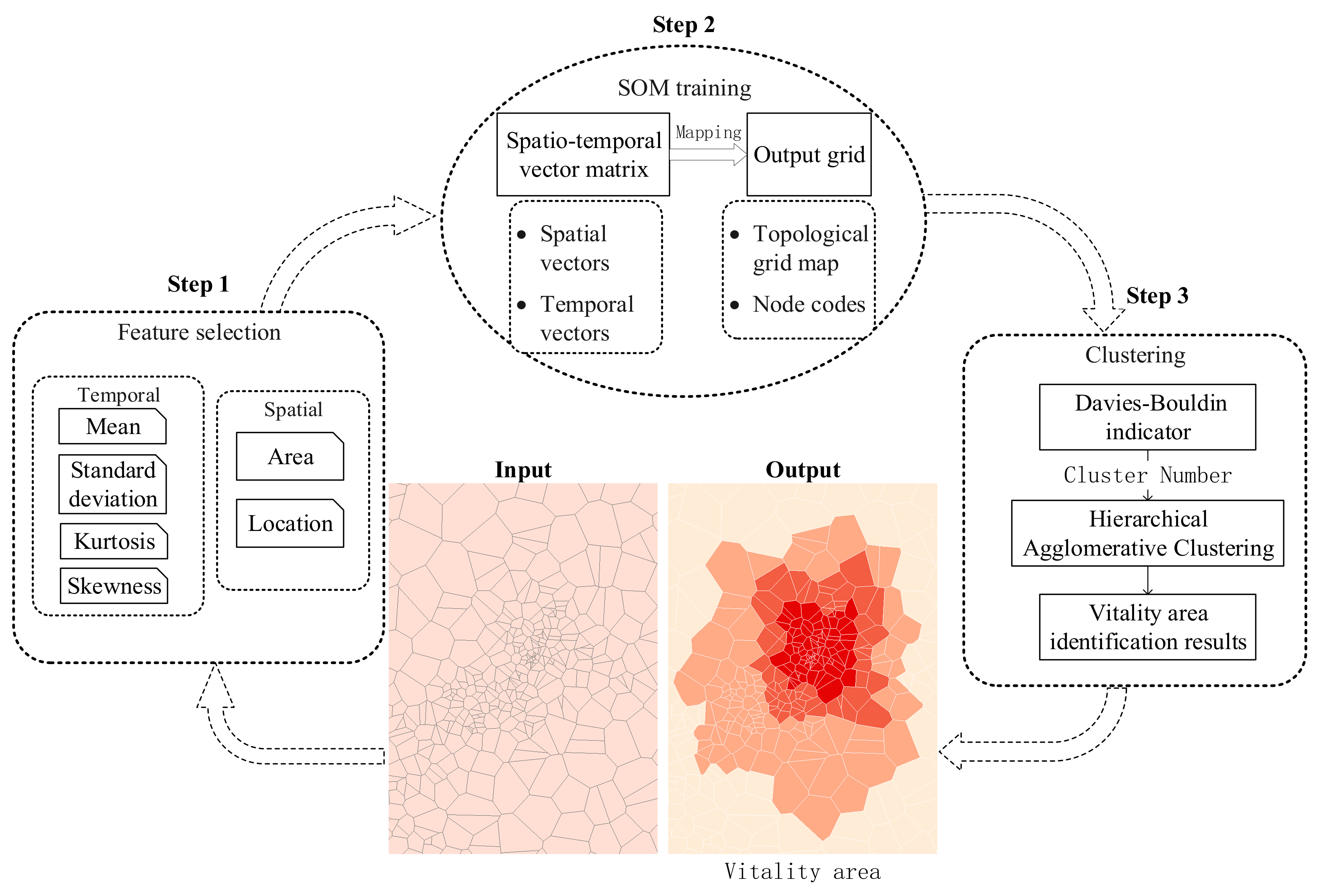
In this paper, dynamic human activity data collected by mobile phone stations were used as a proxy for urban spatiotemporal vitality. The population change dataset inferred by mobile phone base stations together with these stations’ location information constituted the GTS dataset (PSTVD). An urban vitality pattern recognition method based on the self-organizing map (SOM) [37,38] model integrating spatial and temporal characteristics is proposed in this paper. The SOM model, which is a neural network model known as an excellent tool in the exploratory phase of data mining and pattern recognition [39], projects the multidimensional input space on a low-dimension regular grid through an iterative competitive training. Through the SOM feature training extracted from PSTVD and further abstraction of the training output grid, this method was applied to upscale from individual station data to regional patterns, and adjacent stations with similar time variation characteristics were automatically identified as an urban vitality area. The implementation framework consisted of three core steps, as shown in Figure 1.
3.1. Selection of Spatial and Temporal Feature Vectors of Urban Vitality
3.1.1. Spatial Feature Selection
Mobile phone base stations are not uniformly distributed in the city. Generally, the density of base stations in the main urban area is higher than that in other urban areas. As a result, the coverage of each base station varies. The area covered by each base station was taken as a spatial feature factor because the semantics represented by the same urban vitality strength (population of human activities) were different under different areas. Extracting this feature could prevent a base station with similar population dynamic changes but large differences in coverage areas from being identified as the same vitality area because they had different population activity strengths.
Meanwhile, the urban vitality of different regions is closely related to their spatial location. Generally, the closer the region is to a city center, the more significant the vitality characteristics will be. Therefore, this study took the spatial distance between base stations and the central point of the urban central business district (CBD) as another spatial feature factor. The addition of this feature factor could make the area covered by the adjacent base station in space more likely to be identified as the same vitality area.
3.1.2. Time Series Feature Selection
Time series pattern analysis and time series classification include instance-based and feature-based methods [40]. The former is that, when the pattern of a short time series is known, a new time series can be classified by matching them to similar instances of time series with a known classification. In this context, the similarity between the two time series is evaluated by calculating the Euclidean distance or correlation coefficient between the time-ordered measurements themselves. The amount of human activity in different regions within a day shows significant differences [41,42], and urban vitality studies based on PSTVD face time series with complex, unknown patterns.
By adopting the feature-based time series pattern analysis method, this paper selected four statistical features of time series—mean, standard deviation, skewness, and kurtosis—and integrated them into feature vectors of urban vitality pattern mining. These four statistical features reflected the global structural characteristics of the time series of vitality value and distinguished the level of vitality and the distribution of the values in the frequency domain.
● Mean
The mean value represents the central trend of time series and reflects the overall level of vitality in the region. For a time series the mean value is , where represents the length of the time series, and denotes the vitality value of the th period.
● Standard Deviation
Standard deviation is a measure used to describe the degree of dispersion of a dataset. It reflects the stationarity of the vitality time series. For a time series data , the standard deviation is .
● Kurtosis
Kurtosis is a measure of the peakedness or flatness of the value distribution relative to the normal distribution. For a time series data , the kurtosis coefficient is . The kurtosis for a normal distribution is zero. The kurtosis can describe the steepness of the distribution pattern. When the kurtosis is greater than zero, the data show a leptokurtic and thick-tailed distribution. At this point, the vitality values are scattered on both sides of the mean. When the kurtosis is less than zero, the data are represented as platykurtic, and the vitality values are mostly concentrated around the mean value. At the same , the greater the kurtosis coefficient is, the more extreme the values in the data are.
● Skewness
Skewness is a measure of symmetry, indicating the asymmetry of values around the mean value. For a time series data , the skewness coefficient is . The skewness for a normal distribution is zero. At this point, the distribution of the vitality values is symmetric along both sides of the mean value. When the skewness is greater than zero, the data are skewed right, which means the vitality value is concentrated in the lower part. On the contrary, a negative skewness means that the left tail is heavier than the right tail and that the vitality value is concentrated in the higher part.
3.1.3. Spatial and Temporal Feature Vectors of Urban Vitality
The above time and space dimension indexes were combined to form the input feature vectors of the SOM model. Thereby, the spatial dimension and temporal dimension were merged to mine the regional pattern urban vitality based on the PSTVD, which contains a large number of mobile phone stations. Let the size of PSTVD be , the spatial dataset be expressed as , and the time series data be expressed as :
where . The statistical time interval of the number of people in each station is , and a day is divided into time periods.
The spatial and temporal feature vectors matrix of all objects is , and the matrix size is , which means there are objects and each object contains vectors, where . The composition of the matrix is
where the first two are spatial feature vectors. represents the area of the object, and represents the distance of the object from the CBD of the city center. The last four are the temporal feature vectors, which are the statistical indicators of the mean, standard deviation, kurtosis, and skewness, respectively. In order to make the feature vectors of different dimensions comparable, it was necessary to normalize this feature vector matrix.
3.2. SOM Model Construction for Spatiotemporal Pattern Mining of Urban Vitality
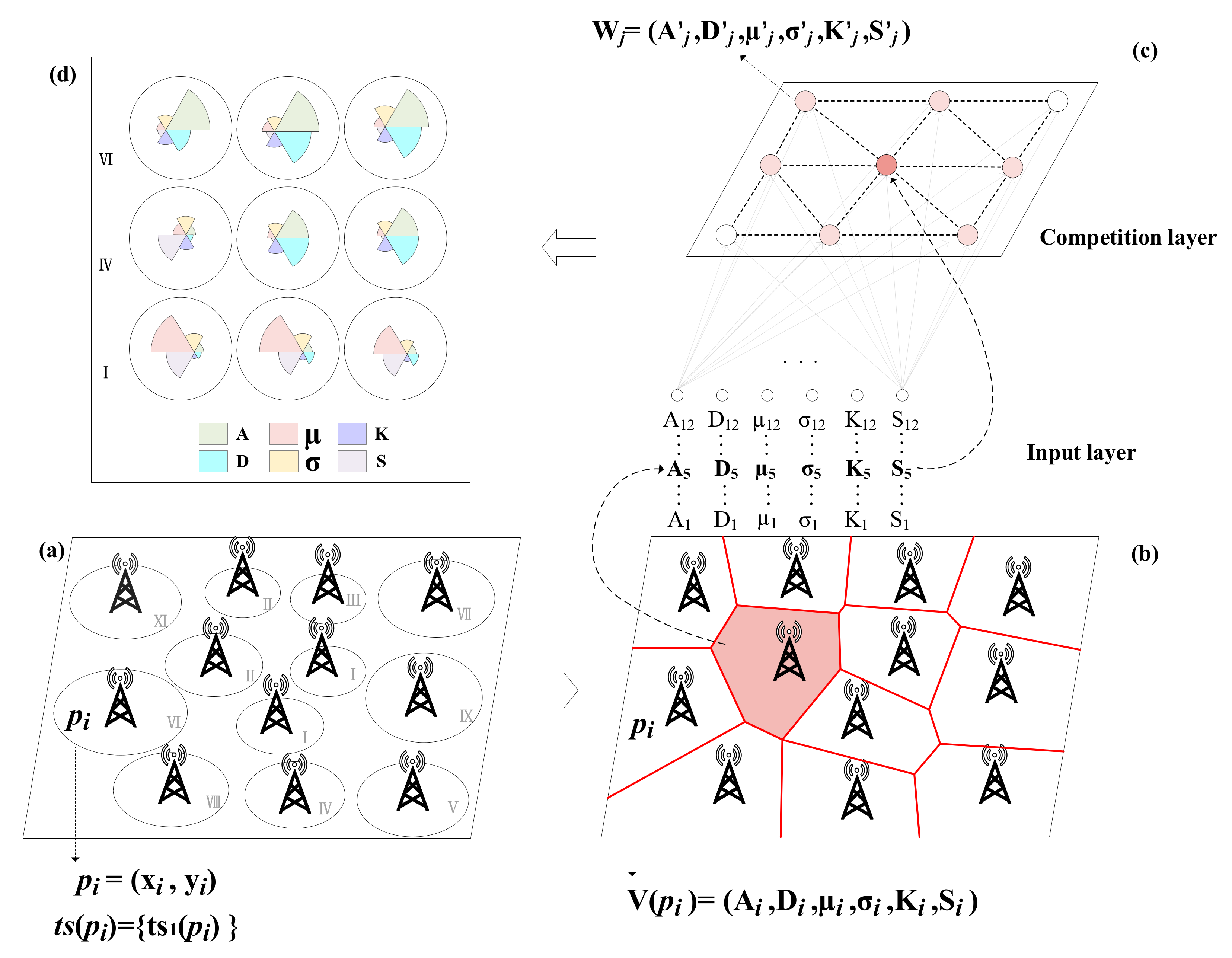
The key to urban vitality pattern mining based on an SOM neural network is the training of the SOM neural network. Based on the method in Section 3.1, the vector matrix of vitality feature was constructed as the input layer of SOM. A 2-D grid network that was either hexagonal or rectangular was used to represent a large number of high-dimensional feature input data abstractly, which required repeated iterations and updates. Figure 2 is an abstract representation of the SOM model training for urban vitality spatiotemporal pattern mining. The specific training process is as follows:
- The weight of each neuron in the SOM network competition layer is initialized by a random function, which is the same as the structure of the input node. Each node consists of six vectors that describe the spatiotemporal characteristics of an urban vitality unit;
- An instance from the input layer is randomly selected to start the competitive learning of the SOM network, and the distance between the instance and the feature vectors of all the output neurons is calculated. The nearest one is the winning neuron. For example, the red spatial unit in Figure 2b is a randomly selected instance. By calculating the distance between this node and all nodes in the competition layer, the winning neuron is found to be the red node at the center of Figure 2c. The distance calculation method determines the final pattern recognition result. A commonly used method is the sum of squares distance or Euclidean distance. In practice, a custom distance calculation method can be required according to a specific problem. The weighted sum of squares distance is defined in this study to enhance the spatial constraint of pattern recognition, and the equation is
- The feature vector of the winning neuron and its surrounding neurons are updated to make it closer to the input instance. The weight update of the feature vector of the peripheral neurons of the winning neurons will monotonically decrease as the number of iterations increases. The specific method can be expressed aswhere is the neighbor node of the winning neuron. In Figure 2c, there are 6 neighbor neurons represented as light red nodes around the wining neuron. is the learning rate, and is the neighborhood kernel function. They decrease as the number of iterations t increases. is defined aswhere is the initial learning rate, usually set to 0.5, and is an exponential decay constant; is a time constant that equals the maximum number of ; and is the neighborhood kernel function that defines the closeness of a neighborhood neuron to the winning neuron. The function can be Gaussian and defined aswhere and , respectively, represent the winning neuron and the node to be updated in the SOM network, and is the width of the neighborhood function, where is the initial width
- Through iterative learning in the second and third steps, all neurons of the network match one or more input nodes, and the distance between each neuron of the network and its input node becomes increasingly close. When the maximum iteration is reached, the training is complete.
After the above model training, a topologically ordered 2-D grid map reflecting the characteristics of all training samples is obtained, as shown in Figure 2d. Each neuron in the graph is a six-dimensional feature vector describing the spatiotemporal features of urban vitality, and the input node closest to the spatiotemporal feature of the neuron is mapped to the neuron. At the same time, the closer the neurons are in the grid map, the more similar the temporal and spatial characteristics are, and vice versa.
3.3. Urban Vitality Area Identification
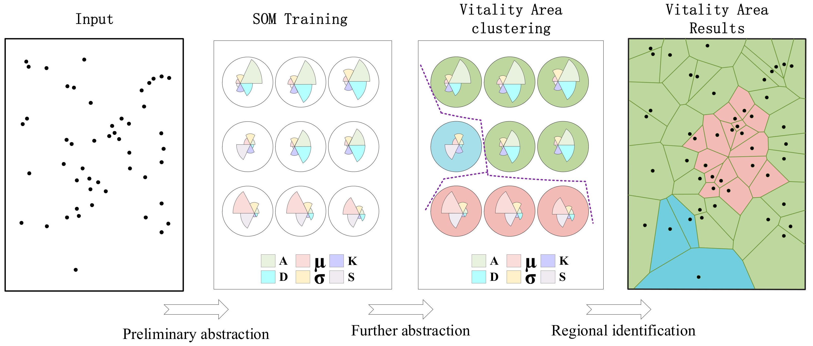
SOM model training has been used to realize the preliminary abstraction of the urban vitality spatiotemporal pattern. A large number of space–time high-dimensional vitality units are mapped into a node in the SOM output layer according to the similarity of their features. According to the size of the dataset, the appropriate grid size is selected for the output layer to abstract the input dataset. Vesanto et al. [39] proposed a rough grid size of , where is the input sample size. When there is a big sample size, a higher abstraction of data is needed. A smaller grid size, such as , is more suitable. A -sized 2-D grid map was used to map the space unit of input vitality, and the features of each output neuron, including two spatial feature vectors and four temporal feature vectors, were described by a codebook. Next, the aggregation pattern of the grid map was extracted to further abstract the vitality pattern, and the nodes with similar temporal and spatial characteristics were aggregated. On this basis, an urban vitality area with the same temporal and spatial characteristics was extracted. The identification process of urban vitality areas is shown in Figure 3. For a similarity measure between objects with definite pattern mining, a classical clustering method with a simple principle and easy implementation, such as k-means and hierarchical clustering, can be used.
For this paper, the hierarchical agglomerative clustering (HAC) method was used for clustering. The weighted sum of squares distance of feature vectors (codebooks) was taken as the similarity degree to achieve cluster merging until all clusters were merged into one class and a dendrogram was generated. The number of clusters clustered was based on the minimum Davies–Bouldin indicator [43], as shown in Equation (8):
where is the number of clusters. This index is aimed at finding , which maximizes the within-cluster distance and minimizes the between-cluster distance. is the average distance between the data in the class and the cluster centroid, and ‖‖ is the distance between the centroid of cluster and cluster . The number of clusters is set to 2 to ( is the number of cluster samples). The datasets are repeatedly clustered using partitive clustering methods such as k-means, and the DB (Davies-Bouldin) indicator is calculated.
4. Experimental Region and Experimental Design
4.1. Case Study Area: Nanjing, China
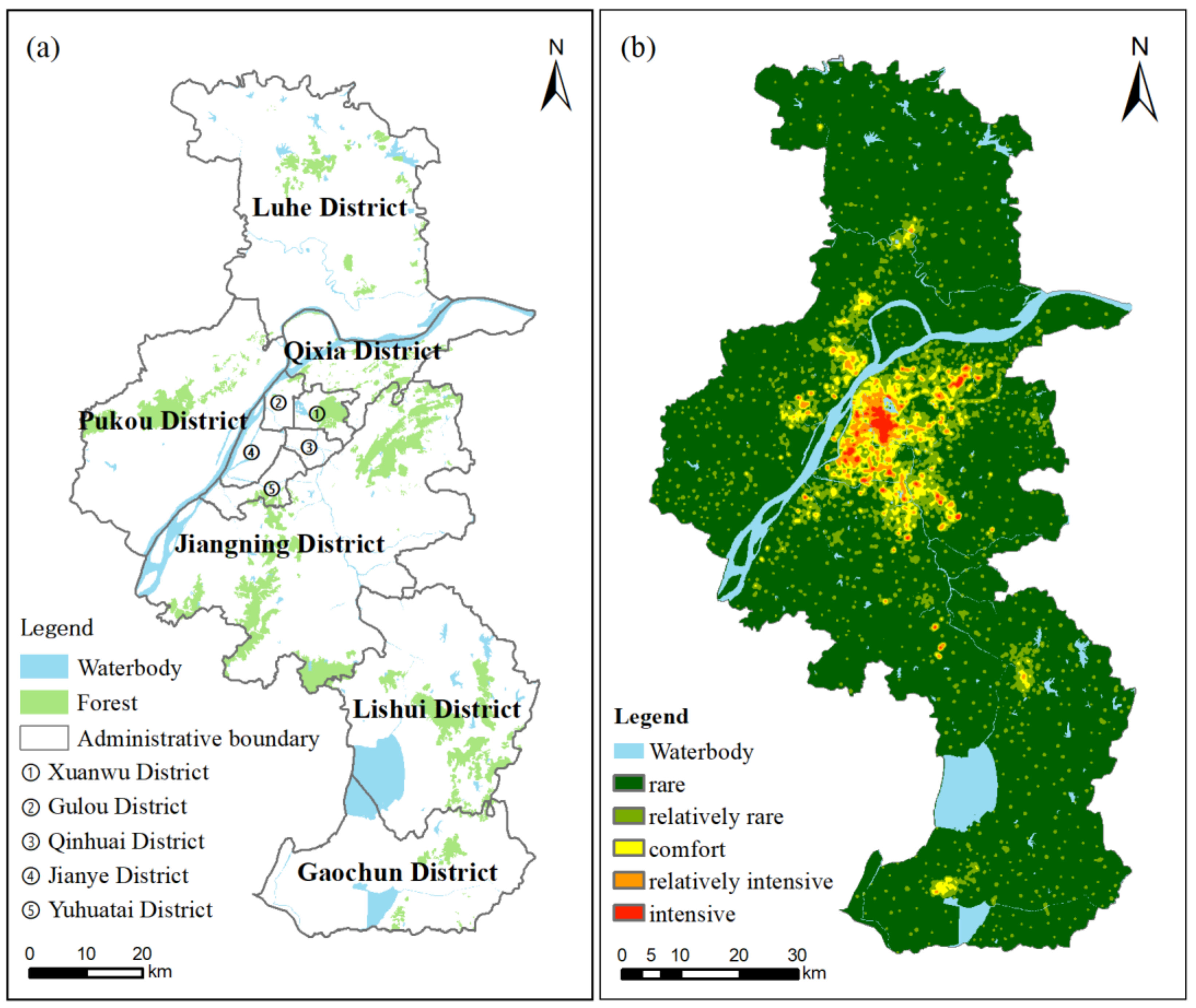
This paper took Nanjing as the research area, which is an important national central city in East China. It is classified as B in the 2018 global city rankings compiled by the Globalization and World Cities (GaWC) Research Network, on par with Berlin and Abu Dhabi [44]. Nanjing covers a total area of 6587 square kilometers and has a jurisdiction of over 11 districts (Figure 4). By the end of 2017, the permanent population of Nanjing was 8.335 million (data from Nanjing Municipal Bureau of Statistics).
4.2. Mobile Phone Data Structure and Data Processing
This study obtained the mobile phone data of the China Telecommunications Corporation from 11 to 17 June 2018 as a data source. Some researchers have employed the term users’ usage detail records (UDRs) data. This records the information from the communication base station connected to the mobile phone when the user makes a call, sends and receives a text message, switches the machine, and switches the base station. In addition, when the user is in a silent state, the base station to which the mobile phone is connected is recorded periodically (every half hour). A total of 1717.42 million records were recorded during the week, including 1219.86 million and 497.56 million records recorded on weekdays and weekends. The daily communication activities of 2.08 million users were recorded, reflecting their movement process in the city with the base stations as the spatial unit. The raw data format is shown in Table 1.
The raw dataset contained all communications data connected to the base stations in Nanjing, including some activity records of passing users. Here, the data of users who only passed through Nanjing on road vehicles, such as high-speed trains or cars, but did not stay in the city or participate in urban life, were excluded, since they did not have a direct impact on the vitality of the city. A passing user was identified by the following two rules: (1) A user that stayed fewer than 5 h on the same day, or (2) a user that displayed an average moving speed exceeding 80 km/h. The records of passing users in the raw dataset were then filtered out.
The division of urban spatial statistical units directly affects the identification results of vitality areas. However, at present, no effective solution has been proposed for the rational division of urban human activity statistical units of mobile phone data. Based on the filtered mobile phone data, after removing rivers and lakes that directly obstruct human activities, the improved Voronoi division method based on density clustering proposed in this paper was used to divide the coverage area of the base stations as the minimum spatial statistical unit. Here, the DBSCAN clustering algorithm was used to merge base stations with a radius of less than 20 m, and the Voronoi division was then performed. Nanjing was divided into 14,236 spatial statistical units. Figure 5 compares the effect of the spatial unit division before and after improvement. The time series of user amounts, which changed every half hour on weekdays and weekends for each base station, were counted, and the GTS dataset of urban vitality was obtained. Finally, according to the space–time feature calculation method in Section 3.1, six space–time feature vectors of each base station working day and weekend were calculated separately. The distance between each base station and the center point of Xinjiekou district in Nanjing CBD and the area of the space unit in each base station coverage area were counted by the distance measurement tool and area calculation tool of ESRI ArcMap 10.2 (ESRI, Redlands, CA, USA). Meanwhile, the mean, standard deviation, kurtosis, and skewness coefficients of each time series were calculated.
4.3. SOM Model Parameters of Nanjing Vitality Analysis
The time–space eigenvectors of each base station on weekdays and weekends were obtained as the input layer data of the SOM. Before carrying out SOM model training, relevant parameters should be determined by combining experimental data and the expected target. Due to a large number of input datasets (14,236 input samples), the number of SOM training nodes with a size of were taken, and an 8 × 15 grid map was constructed to train the vitality space–time feature vector. The grid aspect ratios of 8 and 15 were chosen to approximate the shape of Nanjing. SOM model training parameters are shown in Table 2. After 200 iterations, the SOM network model converged, and each input node on the working day and weekend was mapped to the hexagonal grid, completing the preliminary abstraction of the vitality spatiotemporal pattern.
4.4. POI-Based Land Use Characteristics Evaluation for Vitality Area
Jacobs has pointed out that diversity is an important factor in creating urban vitality [1]. Similarly, in References [7,12,20], it was shown that the higher the mixed land use, the stronger the urban space vitality. In order to explore the land use characteristics of different urban vitality areas, five POI evaluation indicators were adopted to discuss how the allocation of spatial resources affects the vitality of the city: the POI density index, the POI richness index, entropy, the Simpson index, and the max land use type. The calculation methods were as follows:
where represents the number of each POI type, represents the proportion of each type of land use, and n refers to the total number of land use types. The POI density index is decided by the amount of POIs, and this reflects the concentration of land use in space. POI richness is the number of POI categories, so this indicates the diversity of land use types. The exponential of the Shannon entropy is used to evaluate the orderliness of land use. The higher the entropy value is, the stronger the disorder and randomness of the land use will be. The Simpson index takes into account POI richness as well as the relative abundance of different types of POIs, e.g., evenness [20]. The larger the Simpson index value is, the higher the evenness of the land use will be. The above methods measure the characteristics of land use from the dimensions of concentration, richness, diversity, and evenness, while the last indicator is the dominant type of land use used to analyze the vitality area. The equation is
where index() is the position of the maximum value in .
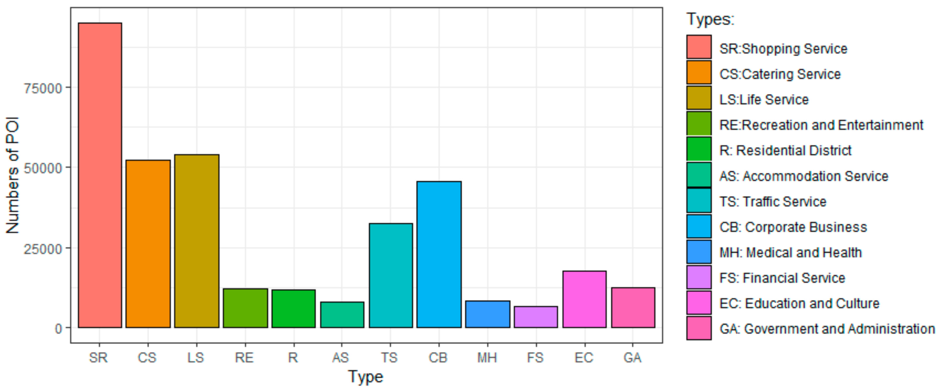
This study obtained navigation-level urban POI data based on the AutoNavi open interface (https://lbs.amap.com/), the largest map navigation service provider in China. The data were updated in August 2018 and have 371,273 POIs covering 24 categories. Since the classification of this data is mainly based on navigation needs, automobile services and traffic facilities are classified in a more detailed way. Referring to the classification standard of urban land use and planning [45], the POI data were integrated into 12 categories here. The number distribution of various POIs in Nanjing is shown in Figure 6.
5. Results and Discussions
5.1. Vitality Area Identification Results of Nanjing
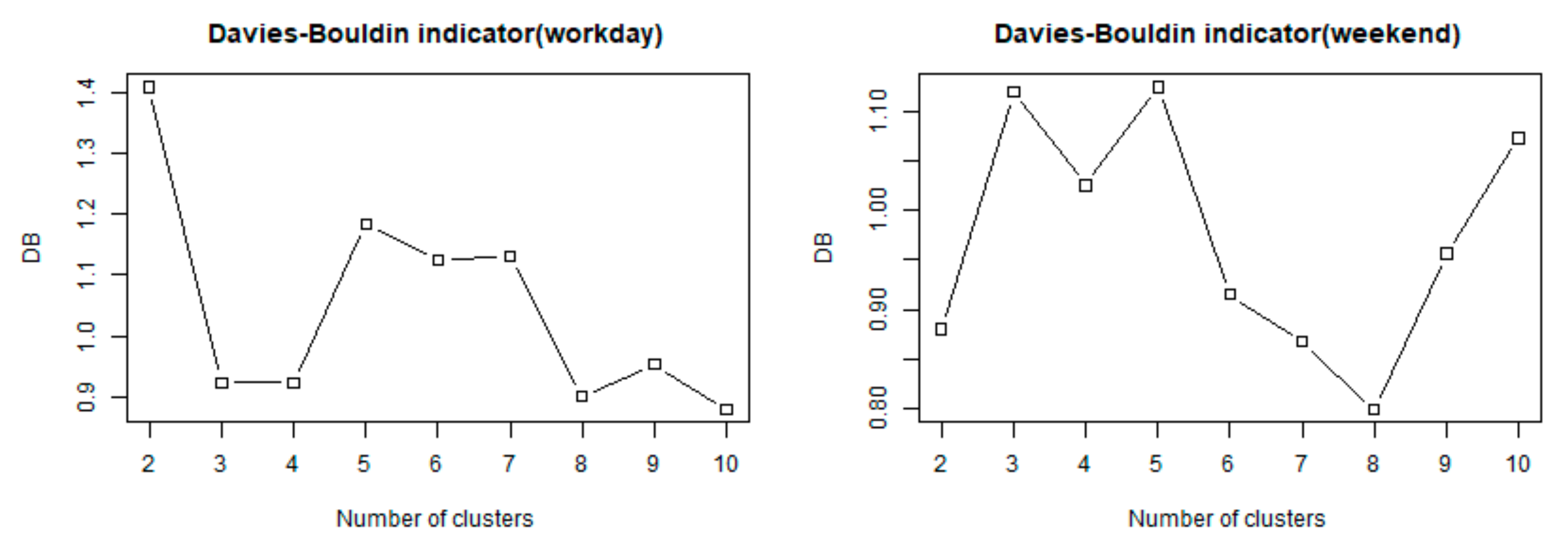
The recognition of urban vitality areas was achieved by clustering the SOM network abstracted by the spatiotemporal pattern. First, we used the k-means method to aggregate the mapped grid maps into 1–10 categories. According to the calculation of the DB indicator, the optimal cluster number of the dataset on the weekdays and the weekend was 10 and 8, respectively. This is shown in Figure 7.
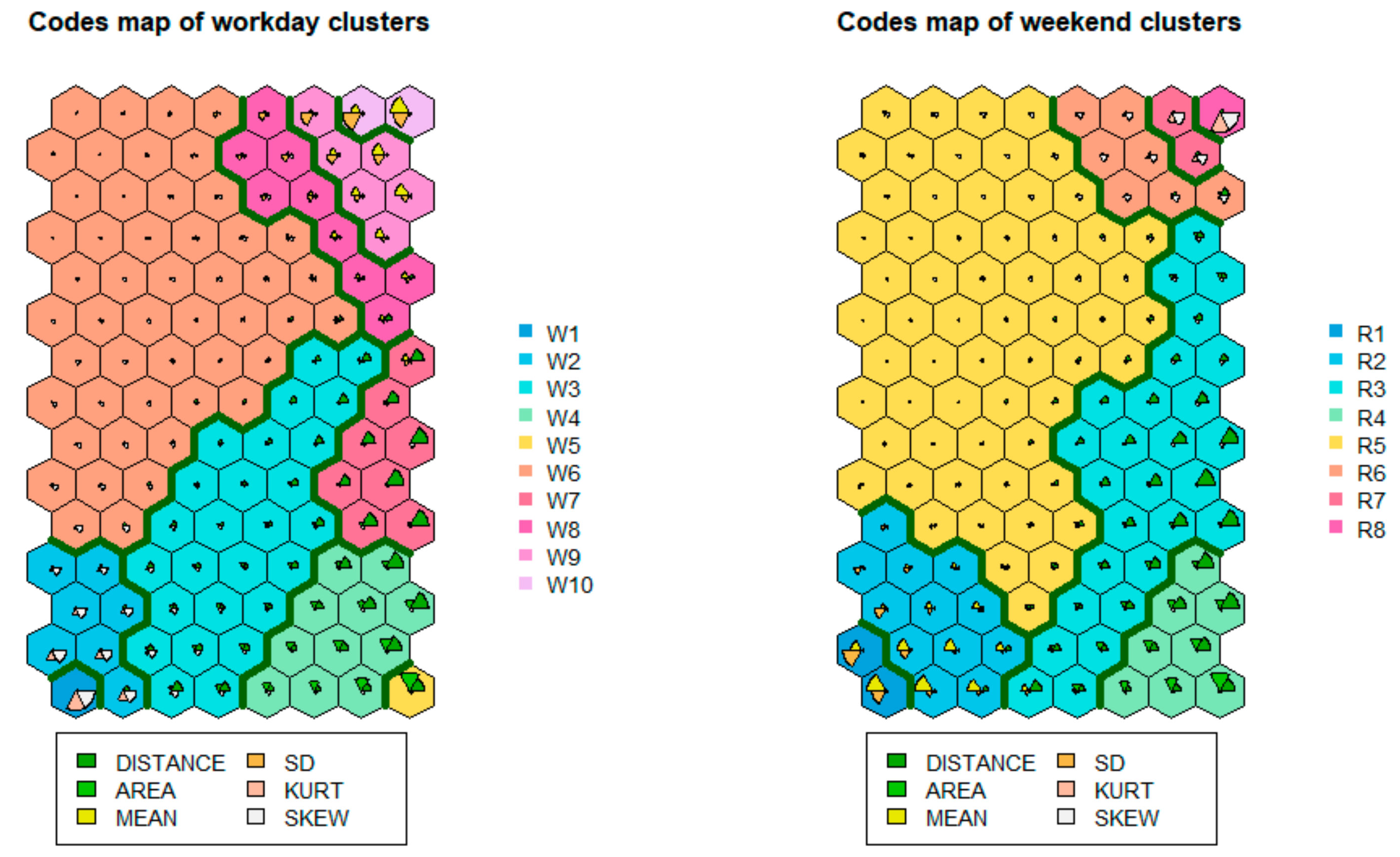
The extraction of the urban vitality area was achieved by clustering the SOM output layer of the 2-D grid map. According to the calculation of the DB index, the optimal cluster number of the dataset was determined to be 10 and 8 for workdays and weekends, respectively. Based on the hierarchical agglomeration clustering method, the SOM output layer network was clustered. The similarity between objects was measured by the weighted sum of squares distance defined in Equation (3), and the proximity between clusters was determined via the Ward method, which maximizes the difference between clusters. Figure 8 shows the clustering results of the SOM network based on HAC clustering. Workdays and weekends were divided into 10 and 8 clusters, respectively, and a cluster formed a vitality area in Nanjing. The spatial–temporal dimensional features of each node are represented in a honeycomb graph composed of hexagonal girds, and the clustering results are represented by different colors. Different clusters are separated by dark green dividing lines. According to the feature image distribution of different clusters, it is not difficult to see that the features of nodes in the same cluster had a high consistency.
Combining the spatial units covered by each input base station point, each input node was spatially visualized according to the clustering result, and the vitality area distribution is shown in Figure 9 and Figure 10. The patches of the same color in the figure represent a vitality area. The dotted line in the figure is the urban–rural spatial layout of the Nanjing Master Plan (2011–2020) from Nanjing’s planning and natural resources bureau [46]. The area within the yellow line is the main urban area, the area within the green line is the metropolitan area, and areas outside the green line are other urban areas.
5.2. Analysis of the Spatial–Temporal Pattern of Vitality Areas in Nanjing
Based on the mining of mobile phone data over a week, the vitality areas of weekdays and weekends in Nanjing were extracted. In general, the overall distribution pattern of the vitality area was similar to the urban structure of Nanjing: The spatial extent of the main urban area and the metropolitan area was roughly consistent with the boundary of the vitality areas. This consistency was more apparent on weekdays, as people engage in a wider range of activities on weekends than on weekdays. The spatial distribution of the vitality area of Nanjing presented a nested structure that spread from the center to the periphery. The continuity of the vitality pattern in the main urban area was lower than that outside the main urban area. The vitality areas of these areas were basically distributed into patches, while the main urban area had some discrete, distributed vitality areas. In the following part, the diurnal variation pattern of urban vitality is analyzed in combination with the time-dimension numerical distribution of each vitality area. The strength, time variation pattern, and spatial heterogeneity rules of urban vitality are discussed.
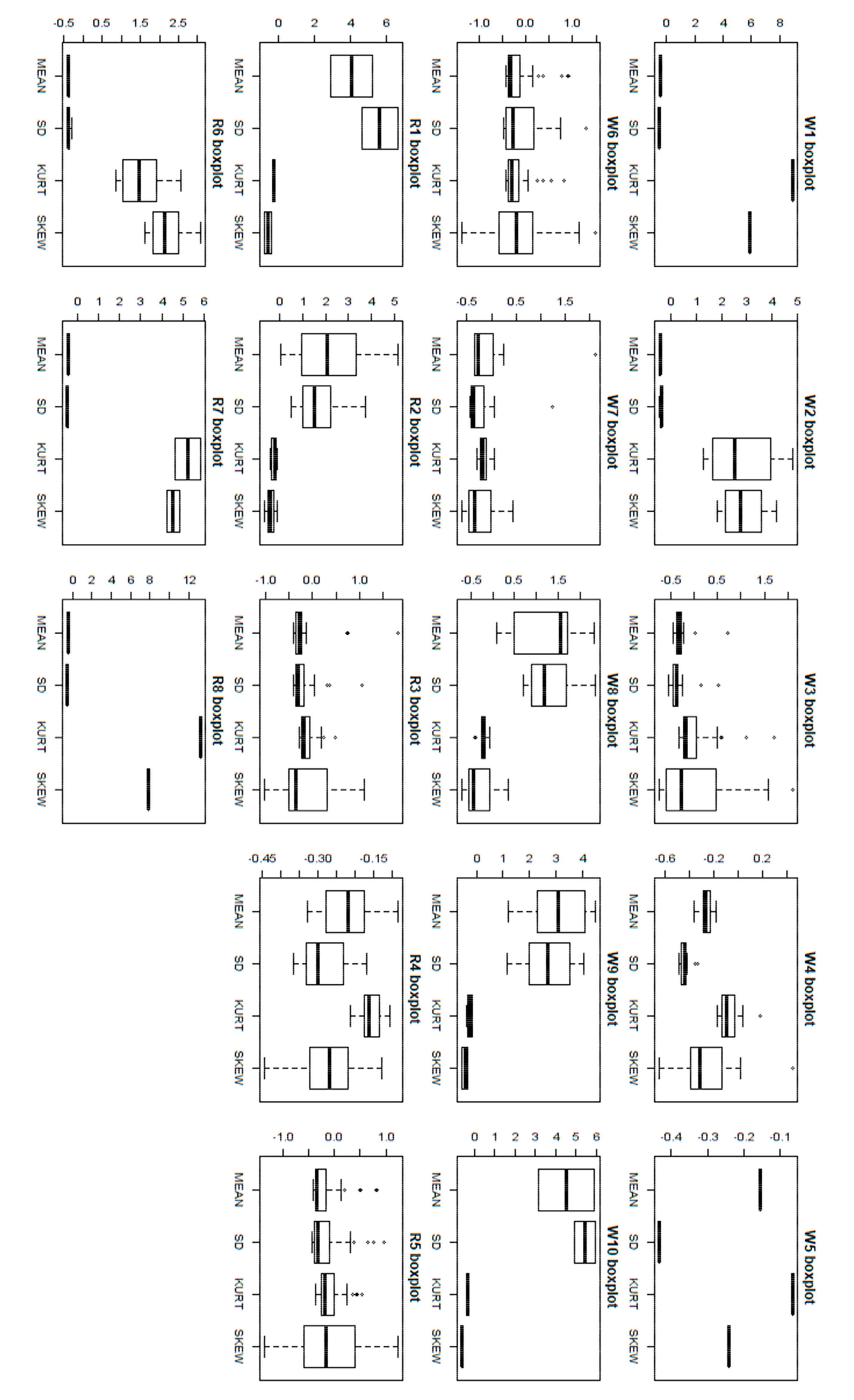
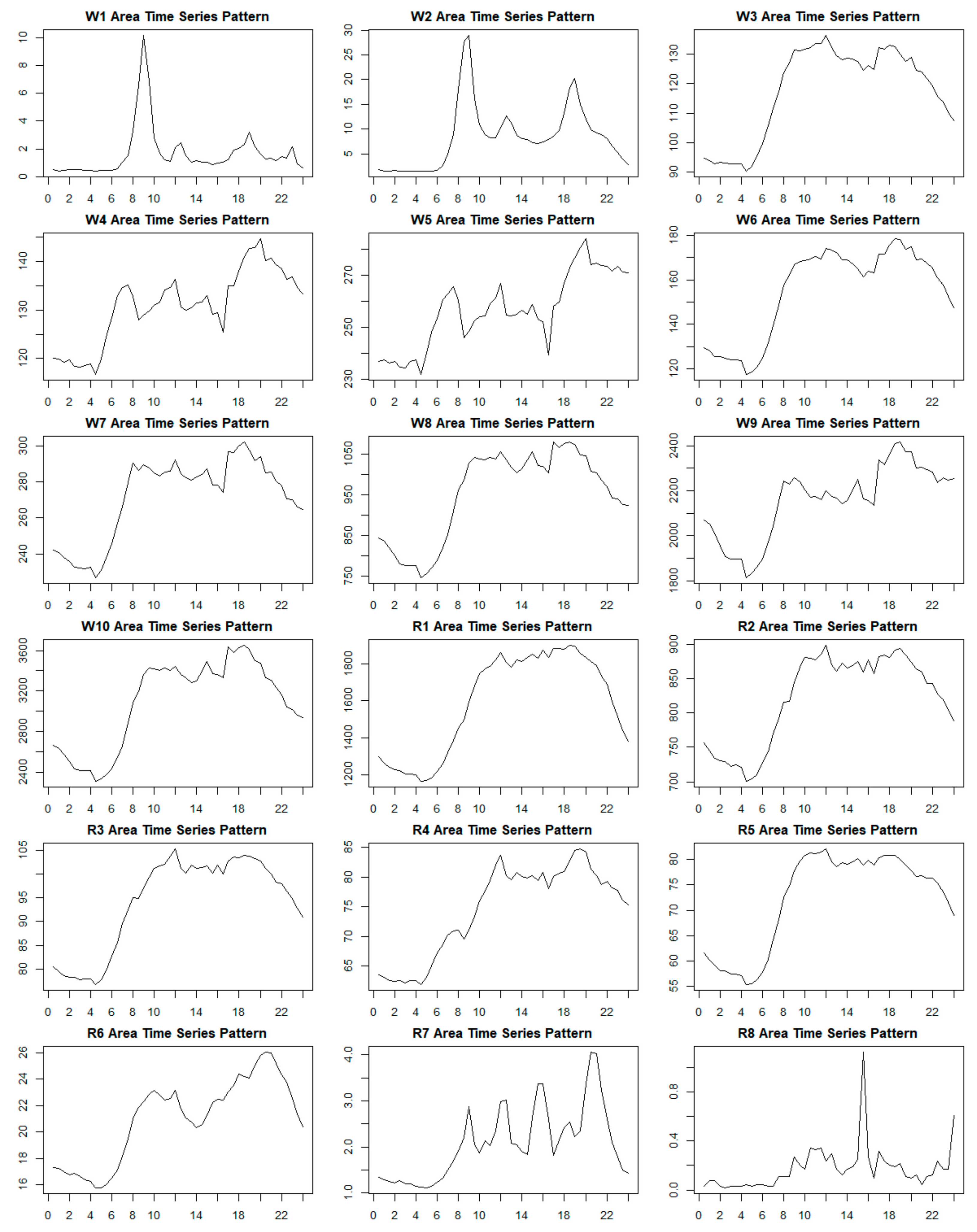
Figure A1 in Appendix A shows the numerical distribution of time-dimensional feature vectors in each vitality area of Nanjing during weekdays and weekends. Since all feature data were standardized before SOM model training, the mean value of each feature vector was zero. Section 3.1.2 explores the relationship between the selected four feature values of the time series and the characteristics of the time series. On this basis, according to the numerical distribution of the time-dimensional features of each vitality area and its spatial distribution, the spatial–temporal patterns of each vitality area in Nanjing on weekdays and weekends are summarized in Table 3. At the same time, based on the time-dimensional characteristics of each vitality area and the time series data of the vitality change, the time-varying characteristic images are fitted to represent the diurnal variation pattern of each vitality area, as shown in Figure A2 in Appendix B.
Based on Table 3 and the above analysis, the city vitality of Nanjing could be divided into different levels according to the vitality value within one day. On weekdays, W1 and W2 are low-vitality areas (see Figure 9b); W3, W4, W5, W6, and W7 are medium-vitality areas; and W8, W9, and W10 are high-vitality areas (see Figure 9c). On weekends, R1 and R2 are high-vitality areas (see Figure 10b); R3, R4, and R5 are medium-vitality areas; and R6, R7, and R8 are low-vitality areas (see Figure 10c). The distribution of low-vitality areas is more concentrated in the main urban area on weekdays than on weekends, and the area of low-vitality areas on weekends is larger. The high-vitality areas on weekends are more concentrated in the main urban area than on weekdays, and this area is less concentrated than it is on working days. This indicates that the high-vitality area on the weekend is very concentrated, and the intensity of human activities in some areas of the main urban area is very high. People are relatively scattered in the main urban area and nearby areas on weekdays with frequent activities. As for the medium-vitality area, the vibrancy areas of weekdays and weekends have a high degree of overlap. Based on the differences in time dimensions, the division of weekdays is more detailed. Specifically, the spatial distributions of W3 and R3; of W4, W5, and R4; and of W6 and R5 are very consistent, while W7 on working days is subdivided from R3 and R4. R5 and W6 are vibrancy areas occupying part of the main urban area of Nanjing, and the distribution range and area of R5 are significantly larger than those of W6, indicating that the overall activity range of people on the weekend is greater than that on working days, except in the high-vitality areas where human activities are very concentrated.
From the standpoint of the smoothness of the time series, the viability of the weekend is more persistent than the working day. According to the time series changes of the medium-vitality area and the high-vitality area, the vitality changes on working days during the day are more obvious, with characteristics of double or multiple peaks, while the stability of the weekend is greater, and the vitality lasts longer. Compared to weekdays, the first vitality peak of the weekend arrives later. Usually, the peak of vitality is reached at around 8:00 a.m. on weekdays, and the weekend peaks occur about 2 h later. This fits well with people’s work and rest schedules. As shown in Figure A2, people need to work and commute on weekdays, and human activities are clearly divided into working hours and breaks, as indicated by the vibrancy pattern of the W3, W6, and W7 regions. There tend to be leisure and other activities at night (e.g., W9 and W10). Since people usually rest at home or go out for activities on weekends, people’s activities during the day and at night are continuous, and their activities gradually weaken at night, with a single peak of vitality, which is reflected in the high-vitality area and medium-vitality area on weekends. W1, W2, R7, and R8 are low-vitality areas, and their time variation patterns are very confusing and are considered to be noise modes.
5.3. Evaluation of Urban Vitality Characteristics
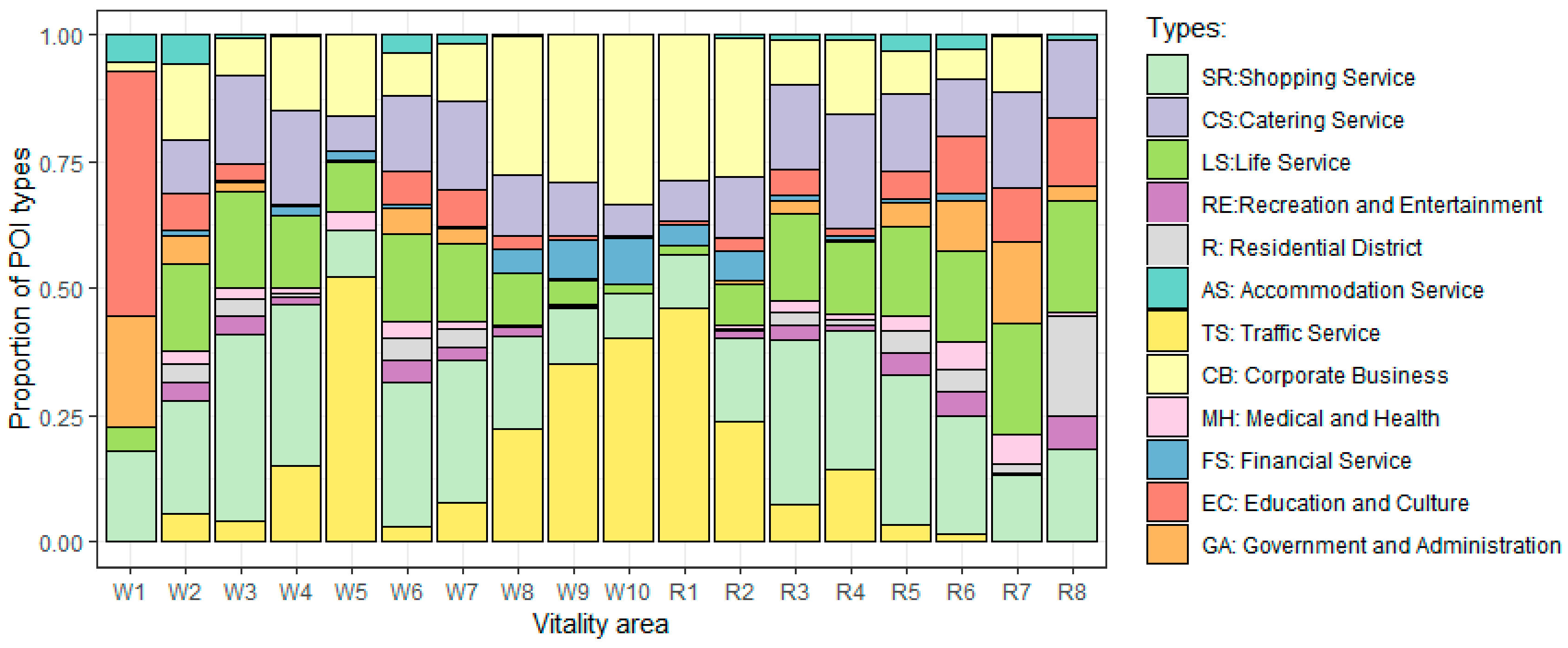
In order to verify the identification results of the vitality areas and explore the driving factors of the vitality spatiotemporal pattern, this paper, based on the POI data of Nanjing, considers the land use characteristics of each vitality area using the land use evaluation indicators. According to the calculation formula of the evaluation index in Section 4.4, the POI numbers, the POI density, the richness, the entropy, the Simpson index, and the max type of POI category in each vitality area were calculated. The results are shown in Table 4. Based on the analysis in the previous section, the vitality levels of each vitality area and the persistence of time patterns are also listed in the table. The POI proportions of different types in each vitality area are shown in Figure 11.
It has already been mentioned that there is a strong consistency in the spatial distribution of the vitality areas between weekdays and weekends. The land use characteristics of these vitality areas can confirm this law. According to Table 4, the calculation results of multiple land use characteristic indexes of W3 and R3; W6 and R5; and W4, W5, and R4 are relatively close. Except for W6, the POI density in the middle- and low-vitality areas is lower than that in the high-vitality area, indicating that the spatial concentration of land use has a significant impact on vitality. At the same time, the high-vitality area has a lower entropy than the low-vitality area, indicating that the orderliness of land use has a greater impact on vitality, i.e., the orderly mixed land use is conducive to enhancing regional vitality. Therefore, although the POI densities of W2, W6, and R5 are relatively high, their entropy is high, and the viability is not as high as it is in W8, W9, W10, R1, and R2. According to the richness index, the Simpson index, and the vitality level, the correlation between land use richness, evenness, and urban vitality is not significant.
According to W9, W10, and R1, the POI type with the largest proportion in the three high-vitality areas is traffic service, which proves that convenient traffic conditions are an important driving force for urban vitality. The other two high-vitality areas on weekdays and weekends, W8 and R2, have the dominant land use type of corporate business, indicating that the enterprise vitality of Nanjing is strong, with a strong relationship between working and residence places, and people are more likely to choose to live close to their workplace. Meanwhile, the common land use characteristics in the vitality areas with high vitality and strong persistence is that they all contain traffic services, corporate business, catering services, shopping services, financial services, and life services. Based on the above analysis, a high POI density, convenient transportation, complete catering, shopping, financial and living services, and proper and orderly mixed land use are important foundations for high vitality. A high richness and randomness of land use are not conducive to stimulating urban vitality.
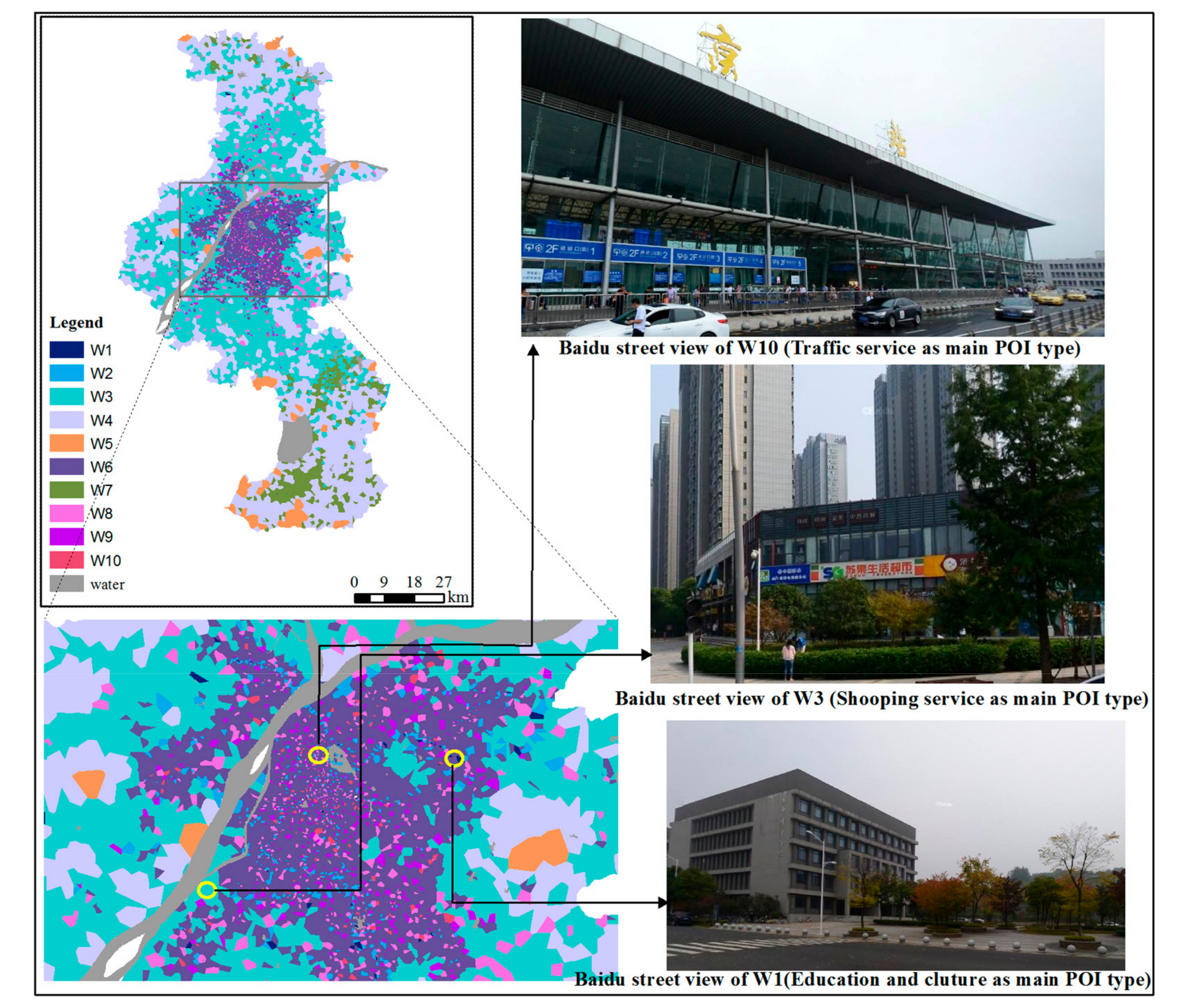
In order to validate the experimental results, we compared the classification results of working days for different levels of vitality areas to the ground truth of corresponding regions. The ground truth was captured by a street view from Baidu Map (map.baidu.com). Here, spatial locations of W10, W3, and W1 were randomly selected as representative of the high-vitality area, medium-vitality area, and low-vitality area, respectively, as shown in Figure 12. The selected location from W10 was Nanjing railway station and automobile transportation station, which is the transportation hub of Nanjing and the distribution center for people to enter and leave Nanjing. This also proved that the main land type of W10 is transportation land, which can create a higher vitality for the city. The selected location from W3 was the community supermarket of a residential community in Nanjing. The POI type in this area mainly carries the function of providing services for life. It was confirmed that the main type of POI in W3 is SR (shopping service). The selected location from W1 was the area of a higher educational institution. It is relatively large, and the activity density of the population is relatively low, so it is an area with relatively low vitality.
5.4. Discussion
In view of the shortcomings of time pattern analysis in current urban vitality quantitative research, this paper constructs an analytical framework for the spatiotemporal pattern mining of urban vitality. Based on the dimensionality reduction characteristics of the SOM algorithm, this framework solves the complex pattern recognition problem of urban human activities in a high space and time dimension. Different from the existing quantitative analysis methods of vitality, the vitality area obtained here was not a predefined spatial area, which gets rid of the limitation of the management unit as the target area of urban spatial vitality measurement. The urban vitality areas extracted are not all spatial continuous areas. At the same time, this compensates for the shortage of time pattern analysis in the existing research. According to the empirical research in Nanjing, the distribution of the sustained, stable, and high-vitality areas is relatively discrete. Therefore, from the perspective of an urban scale, the stimulation of urban vitality is often scattered in some commercial districts, industrial districts, and other areas of the city, and this discrete distribution is more conducive to the balanced and coordinated development of the city.
Next, we discuss the current situation and problems of Nanjing’s development in light of the current spatial structure of Nanjing city planning, the distribution of urban vitality, and the corresponding land use status. In response to these problems, this paper proposes some measures to maintain urban vitality and promote sustainable development.
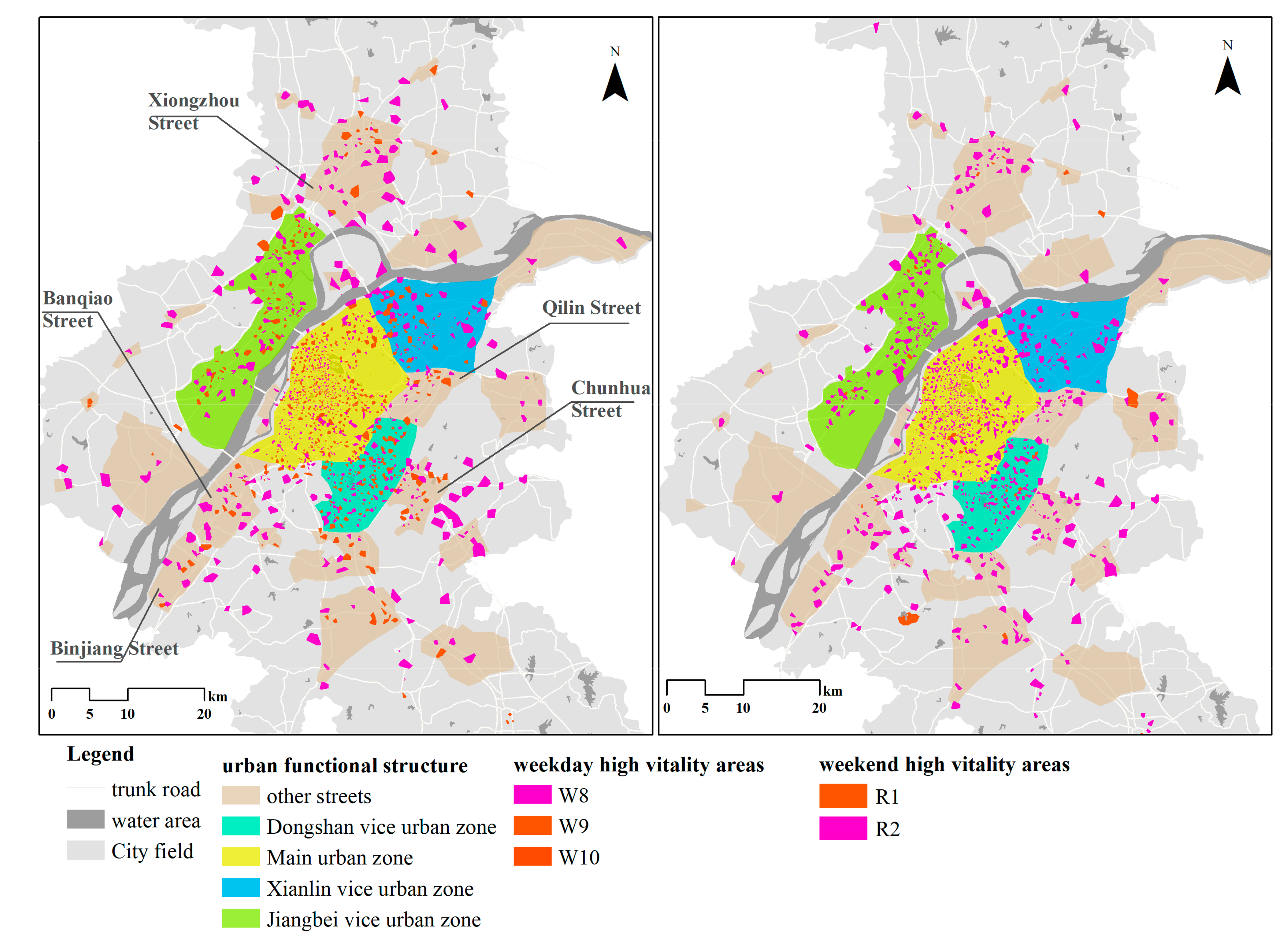
Combined with the urban structure planning of Nanjing and the spatial distribution of the sustainable stable high-vitality area (Figure 13), Nanjing has built a multiaxial radial urban vitality spatial pattern, with the main urban area as the core and the three subcities of Jiangbei, Xianlin, and Dongshan developing in coordination. Taking working days as an example, the high-activity area in the main urban area accounts for 14% of all high-activity areas, the subcity in Jiangbei accounts for 9.3%, the subcity in Xianlin accounts for 7.9%, the subcity in Dongshan accounts for 7.1%, and the other 26 streets account for 30%. According to the analysis of land use characteristics, the construction of roads and other infrastructure plays a crucial role in urban vitality. The main land use in the high-vitality areas in Nanjing is of corporate business. This shows that the relationship between corporate growth and human capital agglomeration is closely related to urban vitality. The integrated development of industry and cities has become a key factor to promote the vitality of Nanjing city.
After comparing the land use conditions in the vitality areas between weekdays and weekends, it was found that leisure and entertainment activities do not play a significant role in promoting the vitality of the city in Nanjing. However, cultural leisure activities have a disguised stimulating effect on the improvement of urban vitality [47,48,49]. With high-intensity work, people need time for relaxation and adjustment, in order to promote production efficiency more favorably and improve people’s quality of life at the same time. Especially in recent years, building a livable city in which its residents are happy has become an important theme in the era of rapid urbanization. In addition to the beautification of a city and the construction of hardware facilities, enriching the leisure life of citizens and improving the vitality of urban innovation should become an important goal in future construction and planning in Nanjing.
In order to promote the healthy and sustainable development of the city, the following suggestions are put forward for the future planning of Nanjing:
- From the perspective of urban structure, building a multicenter structure is more conducive to enhancing urban vitality and promoting coordinated urban development. At present, Nanjing has initially established a pattern of development of one main city and three subcities along the Yangtze River, and the distribution of urban high-energy areas is basically consistent with the current development pattern. Specifically, as we can see from Figure 4, Xiongzhou Street in the north, Binjiang Street and Banqiao Street in the southwest, and Qilin Street and Chunhua Street in the southeast all present with high vitality, so they can be incorporated into the next key planning and construction areas of Nanjing;
- From the perspective of industrial layout, the transportation industry and catering services industry in Nanjing have been fully developed and have become the main shaping factors of the city’s vitality. However, the leisure and entertainment industry is relatively weak. As a major industry affecting the spiritual life of urban residents, leisure and entertainment facilities and related cultural activities need to be further developed;
- In terms of urban spatial form, high-density service facilities and convenient transportation are the basic conditions that facilitate people’s work and life, while orderly mixed land use has a positive correlation with urban vitality. Therefore, to create a highly sustainable vitality space, it is necessary to rationally plan the land use allocation of urban space units, and it is better to meet the above rules.
6. Summary and Future Work
This paper studied the spatiotemporal characteristics of urban vitality from the perspective of a regional model based on the cleaning, processing, and mining of big data. A clustering method based on the SOM model, which aggregates input data with similar spatiotemporal characteristics into vitality areas, was proposed. This work broke the traditional paradigm of urban spatial vitality analysis based on predefined spatial units. Taking Nanjing as the research area, the vitality areas on weekdays and weekends were identified. The agglomeration size of persistent high-vitality areas was ranked as main city, Jiangbei subcity, Xianlin subcity, and Dongshan subcity. Combined with an analysis of land use characteristics in the vitality areas, it was found that the vitality of Nanjing is mainly related to the production activities of urban residents, while the driving effect of leisure and entertainment on the vitality of the city is not obvious. In addition, convenient traffic conditions and orderly organization of life-supporting services play a prominent role in driving the vitality of the city.
There were also some limits in the current research. These shortcomings will be addressed in future research. First, the spatial accuracy of urban vitality areas was extracted from mobile phone data. In this study, the distribution of land cover was not fully considered in the division of space units, and only water areas were excluded as unmovable areas for human beings. Land surfaces were idealized as homogeneous spaces to estimate the distribution of people, but the real surface environment is not like this. Therefore, the results of this study tended to identify land-intensive areas as high-vitality areas, while the vitality of areas with sparse land space was often diluted, such as near universities and other areas with scattered buildings. Therefore, the use of reasonable spatial interpolation technology to improve the spatial accuracy of the extraction of vitality is a direction for future research. Nevertheless, this paper analyzed the correlation between urban vitality level and people’s activities from the perspective of land use characteristics and found a correlation between enterprise development and urban vitality. However, the types of people’s activities were not mined to verify this conclusion. Therefore, based on the semantic extraction of human activities, the inner driving force of urban vitality could be deeply analyzed by examining the relationship between the spatiotemporal heterogeneity of production activities, educational activities, leisure activities, and urban vitality. This will provide support for decision-making departments to execute industrial layout planning and coordinate the sustainable development of the city. Finally, limited by the current availability of mobile phone data, this paper obtained data from one week in June as the time window for analysis. Seasonality has a great influence on people’s choice of activities. For example, in spring and autumn, when the climate is pleasant, people are more likely to choose leisure and entertainment on weekends. Therefore, it will be very interesting to analyze the seasonal differences of urban vitality, which will be the direction of our future research.
Author Contributions
Conceptualization, S.L. and Y.L.; Methodology, S.L. and L.Z.; Writing—original draft preparation, S.L.; Writing—review and editing, L.Z.; funding acquisition, L.Z. and Y.L.
Funding
This research was funded by the National Key Research and Development Program of China (2017YFB0503500), the National Natural Science Foundation of China (41571382, 41501496), the Key Laboratory of Spatial Data Mining & Information Sharing of Ministry of Education, Fuzhou University (2017LSDMIS05) and the Priority Academic Program Development of Jiangsu Higher Education Institutions.
Acknowledgments
The experimental data used for this paper were supported by the Jiangsu intelligent insight big data center of China Telecom Corporation Limited.
Conflicts of Interest
The authors declare no conflict of interest.
Appendix A
Figure A1.
Boxplot of eigenvector weight distribution in each vitality area.

Appendix B
Figure A2.
Diurnal pattern of vitality in each vitality area.

References
- Jacobs, J. The Death and Life of Great American Cities; Random House: New York, NY, USA, 1961; ISBN 9781912282661. [Google Scholar]
- Landry, C. Urban vitality: A new source of urban competitiveness. Archis 2000, 12, 8–13. [Google Scholar]
- John, M. Making a City: Urbanity, Vitality and Urban Design. J. Urban Des. 1998, 3, 93–116. [Google Scholar]
- Lynch, K. Good City Form; MIT Press: Cambridge, MA, USA, 1984. [Google Scholar]
- Lanfen, L. The good life: Criticism and construction of urban meaning. Soc. Sci. China 2010, 31, 133–146. [Google Scholar] [CrossRef]
- Hui, C.; Xianghui, W.; Xiqiang, Z.; Shaoli, Z. The evaluation of Chinese urban traffic management system application based on intelligent traffic control technology. In Proceedings of the 2014 ICICTA 7th International Conference on Intelligent Computation Technology and Automation, Changsha, China, 25–26 October 2014; pp. 791–795. [Google Scholar] [CrossRef]
- De Nadai, M.; Staiano, J.; Larcher, R.; Sebe, N.; Quercia, D.; Lepri, B. The Death and Life of Great Italian Cities: A Mobile Phone Data Perspective. In Proceedings of the International World Wide Web Conferences Steering Committee, Montréal, QC, Canada, 11–15 April 2016; pp. 413–423. [Google Scholar] [CrossRef]
- Yue, W.; Chen, Y.; Zhang, Q.; Liu, Y. Spatial Explicit Assessment of Urban Vitality Using Multi-Source Data: A Case of Shanghai, China. Sustainability 2019, 11, 638. [Google Scholar] [CrossRef]
- Jin, X.; Long, Y.; Sun, W.; Lu, Y.; Yang, X.; Tang, J. Evaluating cities’ vitality and identifying ghost cities in China with emerging geographical data. Cities 2017, 63, 98–109. [Google Scholar] [CrossRef]
- Sung, H.; Lee, S.; Cheon, S.H. Operationalizing Jane Jacobs’s Urban Design Theory: Empirical Verification from the Great City of Seoul, Korea. J. Plan. Educ. Res. 2015, 35, 117–130. [Google Scholar] [CrossRef]
- Sung, H.; Lee, S. Residential built environment and walking activity: Empirical evidence of Jane Jacobs’ urban vitality. Transp. Res. Part D Transp. Environ. 2015, 41, 318–329. [Google Scholar] [CrossRef]
- Wu, J.; Ta, N.; Song, Y.; Lin, J.; Chai, Y. Urban form breeds neighborhood vibrancy: A case study using a GPS-based activity survey in suburban Beijing. Cities 2017, 74, 100–108. [Google Scholar] [CrossRef]
- Zheng, Q.; Deng, J.; Jiang, R.; Wang, K.; Xue, X.; Lin, Y.; Huang, Z.; Shen, Z.; Li, J.; Shahtahmassebi, A.R. Monitoring and assessing “ghost cities” in Northeast China from the view of nighttime light remote sensing data. Habitat Int. 2017, 70, 34–42. [Google Scholar] [CrossRef]
- Wu, W.; Wang, J.; Li, C.; Wang, M. The Geography of City Liveliness and Consumption: Evidence from Location-Based Big Data. LSE Research Online Documents on Economics83642, London School of Economics and Political Science. 2016. Available online: http://eprints.lse.ac.uk/83642/1/sercdp0201.pdf (accessed on 25 July 2019).
- Wu, C.; Ye, X.; Ren, F.; Du, Q. Check-in behaviour and spatio-temporal vibrancy: An exploratory analysis in Shenzhen, China. Cities 2018, 77, 104–116. [Google Scholar] [CrossRef]
- He, Q.; He, W.; Song, Y.; Wu, J.; Yin, C.; Mou, Y. The impact of urban growth patterns on urban vitality in newly built-up areas based on an association rules analysis using geographical ‘big data’. Land Use Policy 2018, 78, 726–738. [Google Scholar] [CrossRef]
- Candia, J.; González, M.C.; Wang, P.; Schoenharl, T.; Madey, G.; Barabási, A.L. Uncovering individual and collective human dynamics from mobile phone records. J. Phys. A Math. Theor. 2008, 41, 1–15. [Google Scholar] [CrossRef]
- Liu, L.; Biderman, A.; Ratti, C. Urban Mobility Landscape: Real Time Monitoring of Urban Mobility Patterns. In Proceedings of the 11th International Conference on Computers in Urban Planning and Urban Management, Hong Kong, China, 16–18 2009; pp. 1–16. [Google Scholar]
- Lu, S.; Fang, Z.; Zhang, X.; Shaw, S.-L.; Yin, L.; Zhao, Z.; Yang, X. Understanding the Representativeness of Mobile Phone Location Data in Characterizing Human Mobility Indicators. ISPRS Int. J. Geo-Inf. 2017, 6, 7. [Google Scholar] [CrossRef]
- Yue, Y.; Zhuang, Y.; Yeh, A.G.O.; Xie, J.Y.; Ma, C.L.; Li, Q.Q. Measurements of POI-based mixed use and their relationships with neighbourhood vibrancy. Int. J. Geogr. Inf. Sci. 2017, 31, 658–675. [Google Scholar] [CrossRef]
- Ye, Y.; van Nes, A. Measuring urban maturation processes in Dutch and Chinese new towns: Combining street network configuration with building density and degree of land use diversification through GIS. J. Space Syntax 2013, 4, 18–37. [Google Scholar]
- Zeng, C.; Song, Y.; He, Q.; Shen, F. Spatially explicit assessment on urban vitality: Case studies in Chicago and Wuhan. Sustain. Cities Soc. 2018, 40, 296–306. [Google Scholar] [CrossRef]
- Batty, M. The pulse of the city. Environ. Plan. B Plan. Des. 2010, 37, 575–577. [Google Scholar] [CrossRef]
- Ying, L.; Yin, Z. Quantitative evaluation on street vibrancy and its impact factors: A case study of Chengdu. New Archit. 2016, 1, 52–57. [Google Scholar]
- Xu, X.; Xu, X.; Guan, P.; Ren, Y.; Wang, W.; Xu, N. The cause and evolution of urban street vitality under the time dimension: Nine cases of streets in Nanjing City, China. Sustainability 2018, 10, 2797. [Google Scholar] [CrossRef]
- Dale, A.; Ling, C.; Newman, L. Community vitality: The role of community-level resilience adaptation and innovation in sustainable development. Sustainability 2010, 2, 215–231. [Google Scholar] [CrossRef]
- Kisilevich, S.; Mansmann, F.; Nanni, M.; Rinzivillo, S. Spatio-temporal clustering. In Data Mining and Knowledge Discovery Handbook; Maimon, O., Rokach, L., Eds.; Springer US: Boston, MA, USA, 2010; pp. 855–874. ISBN 978-0-387-09823-4. [Google Scholar]
- Telesca, L.; Cuomo, V.; Lapenna, V.; Macchiato, M. Identifying space-time clustering properties of the 1983-1997 Irpinia-Basilicata (Southern Italy) seismicity. Tectonophysics 2001, 330, 93–102. [Google Scholar] [CrossRef]
- Tianshu, W.U.; Guojie, S.; Xiujun, M.A.; Kunqing, X.I.E.; Xiaoping, G.A.O. Mining geographic episode association patterns of abnormal events in global earth science data. Earth Sci. 2008, 51, 155–164. [Google Scholar] [CrossRef]
- Zhang, P.; Liu, S.; Du, J. A Map Spectrum-Based Spatiotemporal Clustering Method for GDP Variation Pattern Analysis Using Nighttime Light Images of the Wuhan Urban Agglomeration. ISPRS Int. J. Geo-Inf. 2017, 6, 160. [Google Scholar] [CrossRef]
- Nakaya, T.; Yano, K. Visualising crime clusters in a space-time cube: An exploratory data-analysis approach using space-time kernel density estimation and scan statistics. Trans. GIS 2010, 14, 223–239. [Google Scholar] [CrossRef]
- Kulldorff, M.; Heffernan, R.; Hartman, J.; Assunção, R.; Mostashari, F. A space-time permutation scan statistic for disease outbreak detection. PLoS Med. 2005, 2, 216–224. [Google Scholar] [CrossRef]
- Cheng, T.; Haworth, J.; Anbaroglu, B.; Tanaksaranond, G.; Wang, J. Spatiotemporal data mining. In Handbook of Regional Science; Springer: Berlin/Heidelberg, Germany, 2014; pp. 1173–1193. ISBN 9783642234309. [Google Scholar]
- Zhang, P.; Huang, Y.; Shekhar, S.; Kumar, V. Correlation analysis of spatial time series datasets: A filter-and-refine approach. Adv. Knowl. Discov. Data Min. 2003, 532–544. [Google Scholar] [CrossRef]
- Birant, D.; Kut, A. ST-DBSCAN: An algorithm for clustering spatial-temporal data. Data Knowl. Eng. 2007, 60, 208–221. [Google Scholar] [CrossRef]
- Wu, X.; Zurita-Milla, R.; Kraak, M.J. Co-clustering geo-referenced time series: Exploring spatio-temporal patterns in Dutch temperature data. Int. J. Geogr. Inf. Sci. 2015, 29, 624–642. [Google Scholar] [CrossRef]
- Kohonen, T. Self-organized formation of topologically correct feature maps. Biol. Cybern. 1982, 43, 59–69. [Google Scholar] [CrossRef]
- Kohonen, T. The self-organizing map. Proc. IEEE 1990, 78, 1464–1480. [Google Scholar] [CrossRef]
- Vesanto, J.; Alhoniemi, E. Clustering of the self-organizing map. IEEE Trans. Neural Netw. 2000, 11, 586–600. [Google Scholar] [CrossRef]
- Fulcher, B.D.; Jones, N.S. Highly comparative feature-based time-series classification. IEEE Trans. Knowl. Data Eng. 2014, 26, 3026–3037. [Google Scholar] [CrossRef]
- Ahas, R.; Aasa, A.; Yuan, Y.; Raubal, M.; Smoreda, Z.; Liu, Y.; Ziemlicki, C.; Tiru, M.; Zook, M. Everyday space–time geographies: Using mobile phone-based sensor data to monitor urban activity in Harbin, Paris, and Tallinn. Int. J. Geogr. Inf. Sci. 2015, 29, 2017–2039. [Google Scholar] [CrossRef]
- García-Palomares, J.C.; Salas-Olmedo, M.H.; Moya-Gómez, B.; Condeço-Melhorado, A.; Gutiérrez, J. City dynamics through Twitter: Relationships between land use and spatiotemporal demographics. Cities 2018, 72, 310–319. [Google Scholar] [CrossRef]
- David, L.D.; Donald, W.B. A Cluster Separation Measure. IEEE Trans. Pattern Anal. Mach. Intell. 1979, 1, 224–227. [Google Scholar] [CrossRef]
- World City Classification Ranking According to GaWC. Available online: https://www.lboro.ac.uk/gawc/world2018t.html (accessed on 25 July 2019).
- Wang, K.; Zhao, M.; Lin, J.; Zhang, J.; Jin, D.X.; Xu, Z.; Chu, J.Q.; Li, X.Y.; Xu, Y.; Xie, Y.; et al. Land(GB50137-2011), S. of D. Standardization Administration of the People’s Republic of China (2011). City Plan. Rev. 2012, 36, 42–48. [Google Scholar]
- Nanjing Planning and Natural Resources Bureau Nanjing Urban Master Plan (2011–2020). Available online: http://ghj.nanjing.gov.cn/ztzl/ghbz/ztgh/201705/P020181025388662691810.jpg (accessed on 25 July 2019).
- Baycan, T.; Nijkamp, P. A socio-economic impact analysis of urban cultural diversity: Pathways and horizons. In Migration Impact Assessment New Horizons; Edward Elgar: Cheltenham, UK, 2012; pp. 175–202. [Google Scholar]
- Jing, Y.; Liu, Y.; Cai, E.; Yi, L.; Zhang, Y. Quantifying the spatiality of urban leisure venues in Wuhan, Central China–GIS-based spatial pattern metrics. Sustain. Cities Soc. 2018, 40, 638–647. [Google Scholar] [CrossRef]
- Keane, M. Creative industries in China: Four perspectives on social transformation. Int. J. Cult. Policy 2009, 15, 431–443. [Google Scholar] [CrossRef]
Figure 1.
The urban vitality area identification method based on integrating spatial and temporal characteristics. The first step is to extract the feature vectors representing the temporal and spatial features of each vitality unit as the input of the self-organizing map (SOM) model (Section 3.1). The second step is to build an SOM neural network model to train the feature vectors and obtain a grid map approximating the input data (Section 3.2). The last step is to group similar nodes by the hierarchical clustering method to realize the recognition of the urban vitality area (Section 3.3).

Figure 2.
SOM model architecture for urban vitality spatiotemporal pattern mining. As shown in (a) and (b), the input layer here is a region covered by 12 mobile phone base stations, and the input matrix is obtained by extracting spatial–temporal features from each base station. Then, as shown in (c), a grid network of neurons is constructed as the competition layer of the SOM to train the input matrix and map the nodes with similar spatial and temporal characteristics to the output layer. Here, (d) illustrates a code map that is abstracted after the training is completed to represent the urban vitality spatiotemporal pattern of all input objects. The spatiotemporal characteristics of each node are described by a codebook, and the visualization is shown as a pie chart. The more obvious a feature is, the larger its fan radius is. The Roman numerals in (d) and the base stations in (a) represent the mapping relationship between input and output.

Figure 3.
The identification method for an urban vitality area.

Figure 4.
The administrative division of Nanjing (a) and a base station distribution density map of the telecom operator (b). In the map on the right side, the more the color is biased toward red, the higher the base station density in this area.
Figure 4.
The administrative division of Nanjing (a) and a base station distribution density map of the telecom operator (b). In the map on the right side, the more the color is biased toward red, the higher the base station density in this area.

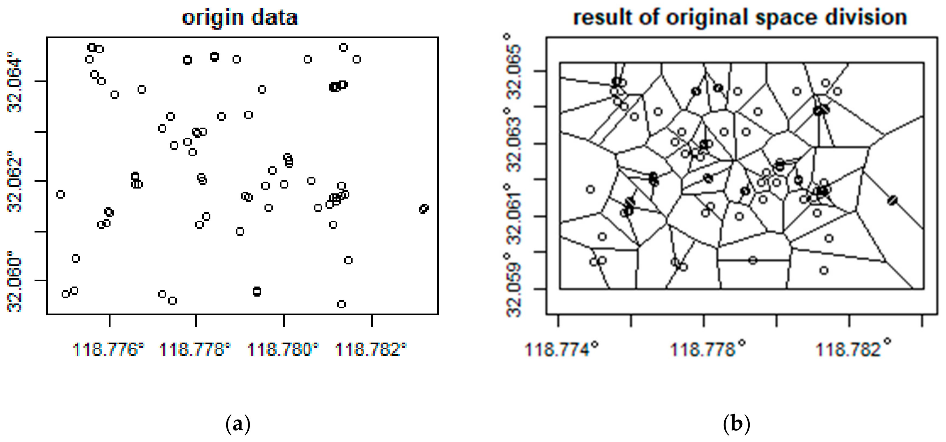
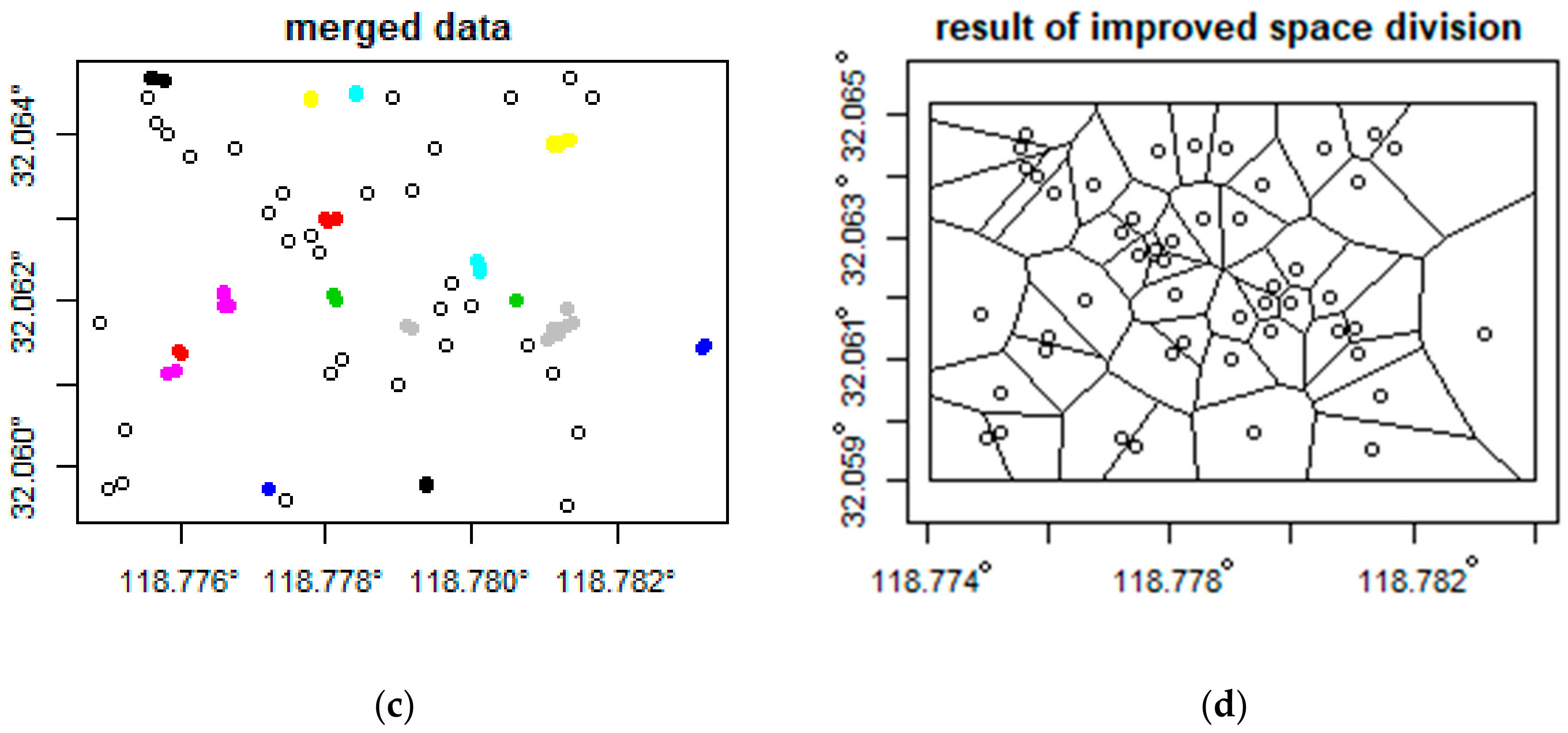
Figure 5.
Comparison of the result of urban vitality spatial statistical unit subdivision before and after using the method proposed in this paper. Here, we simulated 80 points to test this method: (a) is the origin data, and the space division result is shown in (b); (c) shows the merged points used in the DBSCAN method, and (d) is the space division result based on merged points.


Figure 6.
The statistical distribution of points of interest (POIs) by category in Nanjing.

Figure 7.
Determination of cluster numbers of the vitality area for weekdays and weekends. These two figures show the relationship between the DB indicator values and the number of clusters on weekdays and weekends. When values were 10 and 8, respectively, the DB indicator reached its minimum.
Figure 7.
Determination of cluster numbers of the vitality area for weekdays and weekends. These two figures show the relationship between the DB indicator values and the number of clusters on weekdays and weekends. When values were 10 and 8, respectively, the DB indicator reached its minimum.

Figure 8.
The visualization of the SOM grid cluster results of the vitality area for weekdays and weekends.
Figure 8.
The visualization of the SOM grid cluster results of the vitality area for weekdays and weekends.

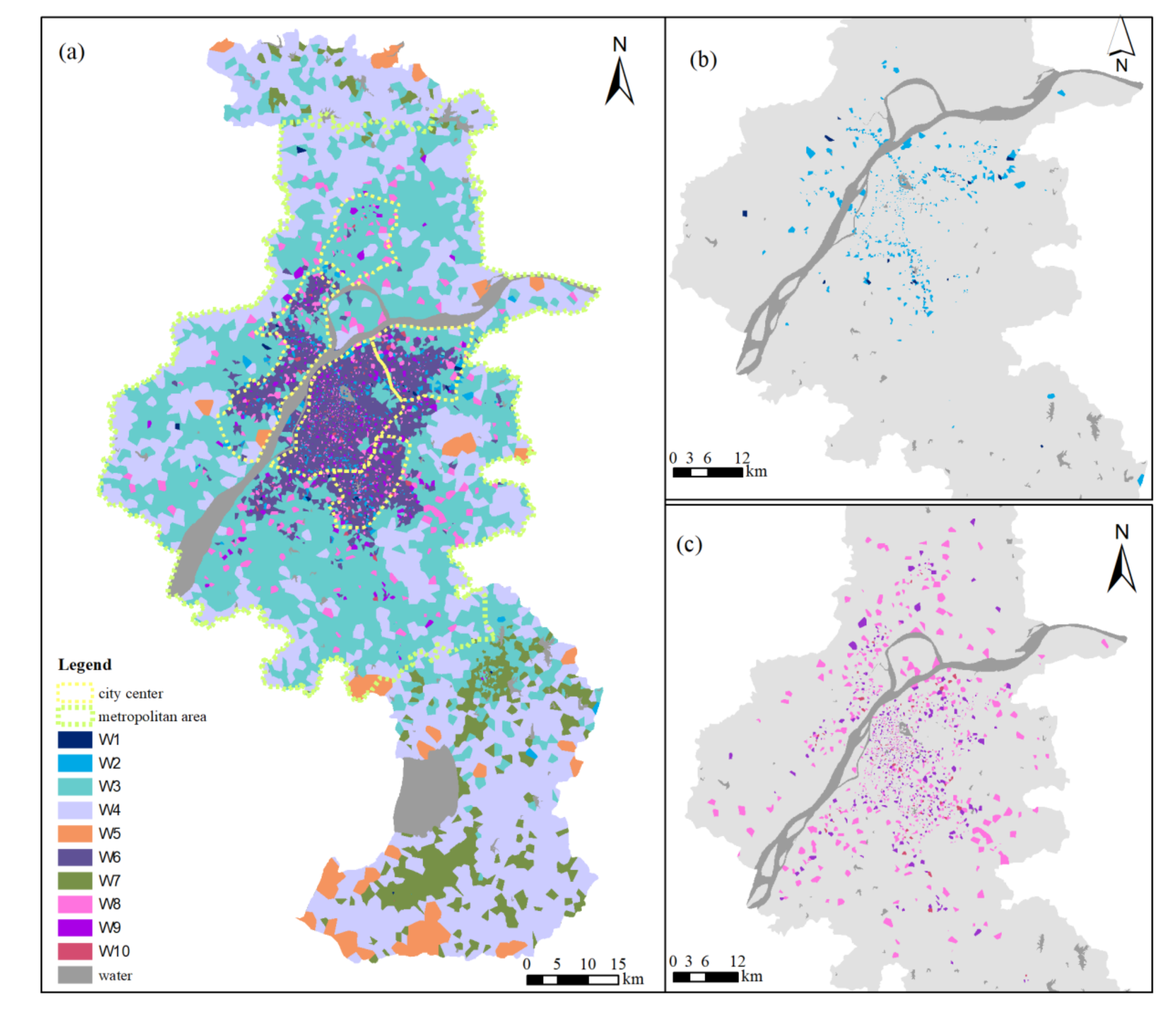
Figure 9.
Spatial distribution of vitality areas in Nanjing during working days. Here, (a) shows the distribution of all vitality areas on working days; (b) shows the spatial distribution of the vitality areas W1 and W2; and (c) shows the spatial distribution of the vitality areas W8, W9, and W10.
Figure 9.
Spatial distribution of vitality areas in Nanjing during working days. Here, (a) shows the distribution of all vitality areas on working days; (b) shows the spatial distribution of the vitality areas W1 and W2; and (c) shows the spatial distribution of the vitality areas W8, W9, and W10.

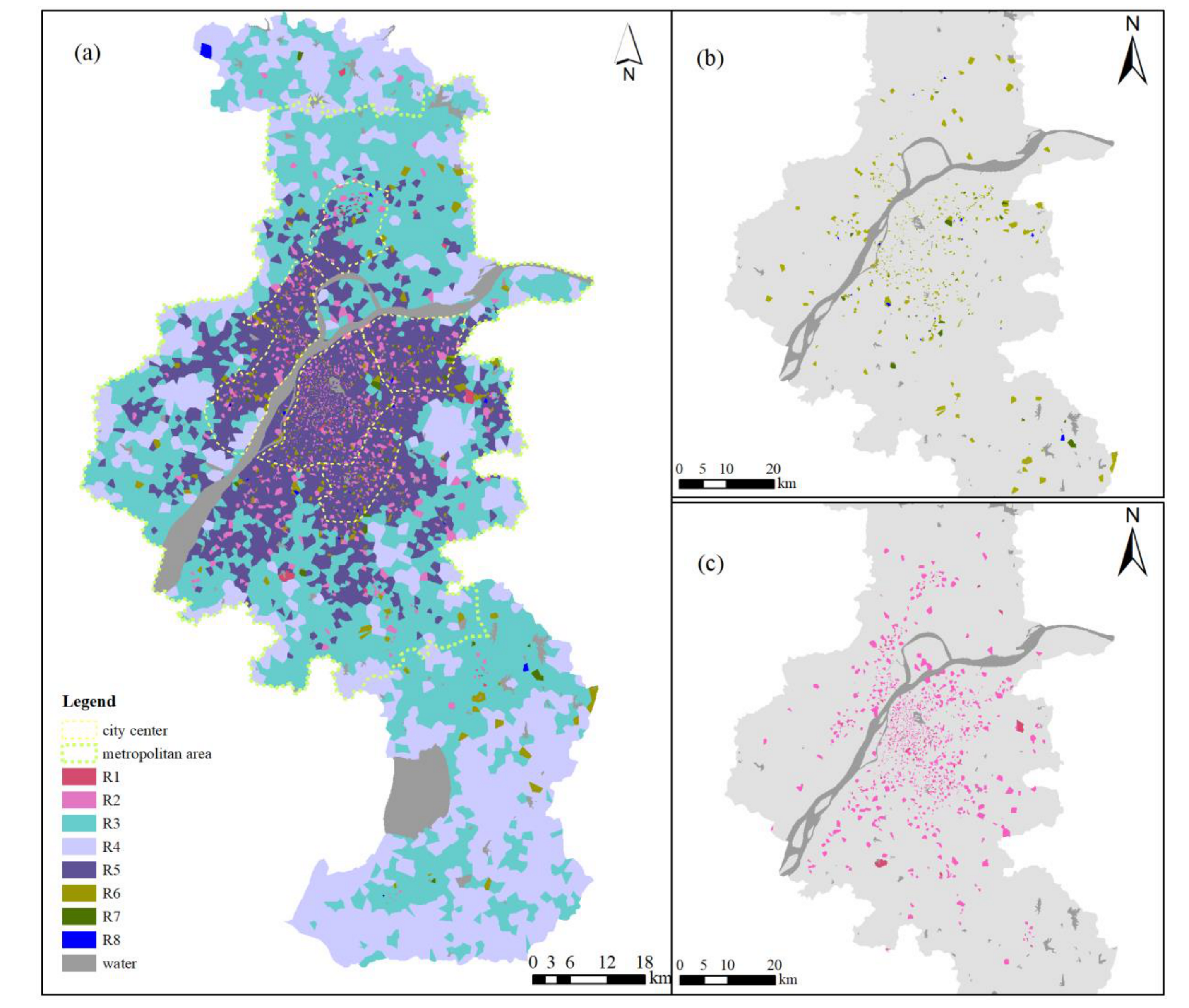
Figure 10.
Spatial distribution of vitality areas in Nanjing during weekends. Here, (a) shows the distribution of all vitality areas on the weekends; (b) shows the spatial distribution of the vitality areas R6, R7, and R8; and (c) shows the spatial distribution of the vitality areas R1 and R2.
Figure 10.
Spatial distribution of vitality areas in Nanjing during weekends. Here, (a) shows the distribution of all vitality areas on the weekends; (b) shows the spatial distribution of the vitality areas R6, R7, and R8; and (c) shows the spatial distribution of the vitality areas R1 and R2.

Figure 11.
The proportion of POI types in each vitality area.

Figure 12.
Case validation with the ground truth for different levels of vitality areas (working days).
Figure 12.
Case validation with the ground truth for different levels of vitality areas (working days).

Figure 13.
Overlay of high-vitality areas and urban structure planning.


Table 1.
Raw data field composition.
| Fields | Description |
|---|---|
| Time | Data submission time; data format is “yyyy-mm-dd hh24:mm:ss”. |
| IMSI | International mobile user identification code. |
| StationID | Unique identification code of mobile phone base station. China Telecom has more than 18,000 base stations in Nanjing. The spatial distribution of the base stations is shown in Figure 4. |
| Longitude | Base station longitude. |
| Latitude | Base station latitude. |
Table 2.
SOM parameters of spatial–temporal vitality pattern training.
| SOM Parameters | Vitality Training SOM Net |
|---|---|
| Grid size | 8 15 |
| Grid topo | Hexagonal |
| Iteration times | 200 |
| Distance measure | The weighted sum of squares distance as shown in Equation (3); here, set parameter and |
| Neighborhood kernel function | Gaussian |
| alpha (learning rate) | (0.05, 0.001) |
Table 3.
A general description of the characteristics of spatiotemporal patterns of each vitality area.
Table 3.
A general description of the characteristics of spatiotemporal patterns of each vitality area.
| Vitality Area | Area (km2) | Description |
|---|---|---|
| W1 | 6.7 | W1 is a low-vitality area scattered in the urban area, with a large kurtosis. The skewness is greater than zero, with a large value variation within the day. |
| W2 | 60.5 | W2 is a low-vitality area distributed in the main urban area of Nanjing. Its characteristics are similar to those of W1. The kurtosis and skewness are greater than zero, and the peakedness feature is not as obvious as it is in W1. |
| W3 | 2265.7 | W3 is mainly surrounded by the main urban area, with a small mean value and a small standard deviation value range. The kurtosis is less than zero, and the skewness is more than zero. It belongs to an area where the overall vitality is not high, but the vitality changes are relatively stable. |
| W4 | 2451.9 | W4 is distributed in the periphery of Nanjing and is far away from the central city. Its mean value is close to that of W3, the standard deviation and skewness are larger than those of W3, the value distribution is more inclined to the lower value part, and the intraday variation is significant. |
| W5 | 223.6 | W5 is distributed along the edge of Nanjing, and its mean and standard deviation are both greater than those of W4. The kurtosis and skewness are close to those of W4. It is a medium-vitality area with very significant changes. |
| W6 | 575.1 | W6 is a vitality area covering a large area of the main urban area. It is a medium-vitality area with stable intraday variations. The kurtosis is less than zero, and the skewness is greater than zero. |
| W7 | 365.3 | W7 mainly includes the Gaochun and Lishui districts of Nanjing city. Its vitality is higher than that of the peripheral non-urban areas. Its kurtosis is close to that of W6, and its skewness is larger than that of W6. Therefore, the time variation of vitality is similar to that of W6, but the parts with lower-vitality values are relatively greater. |
| W8 | 177.8 | W8 is scattered in and around the main urban area, with a high vitality level. Most of its kurtosis is less than zero, its skewness is greater than zero, and most of its vitality values are concentrated near the mean, making it a relatively stable high-vitality area. |
| W9 | 66 | The vitality of W9 is higher than that of W8. The kurtosis is close to that of W8, the skewness is larger, the part with higher vitality is larger, and the duration of vitality is longer. |
| W10 | 13.1 | W10 is the region with the highest-vitality strength on working days. The kurtosis and skewness are mostly less than zero, and the vitality value tends to be concentrated in the high-value range. |
| R1 | 15.4 | R1 is the most energetic area on the weekend and is scattered in the main urban area of Nanjing and the core region of the Gaochun and Lishui districts. Its kurtosis and skewness are less than zero, and the high-vitality period lasts for a long time. |
| R2 | 189.5 | R2 is spread all over the main urban area of the city. Its vitality is second only to R1, with a kurtosis less than zero. The range of skewness is greater than that of R1, and the fluctuation of vitality is higher. |
| R3 | 2545.8 | R3 is distributed in the surrounding area of the main urban area. The vitality level is moderate, the skewness and kurtosis characteristics are similar to those of R2, and the vitality value changes gently. |
| R4 | 1968.7 | R4 is distributed outside the urban area. The overall vitality is slightly lower than R3, and the intraday fluctuation of vitality is relatively larger. |
| R5 | 1371.7 | R5 covers a wide range of the main urban area, and its vitality is general. The kurtosis is close to that of R3, and the skewness is slightly higher than that of R3. The vitality lasts longer, and the fluctuations are less frequent during the day. |
| R6 | 93.9 | R6 is a low-vitality area that is mainly distributed in the main urban area. The kurtosis and skewness are greater than zero, and the vitality value is mostly biased toward the lower part. |
| R7 | 13.5 | R7 is a low-vitality area scattered in different areas of the city. Its kurtosis and skewness values are large, and the intraday variation of vitality is obvious. |
| R8 | 7.2 | R8 is also a cold-vitality area scattered in the city. The kurtosis and skewness are both greater than zero, the kurtosis is higher than R7, and the amplitude of the vitality change is very large. |
Table 4.
Calculation results of land use characteristics in active areas on weekdays and weekends.
| Area | Level | Persistence | POI Indicators | |||||
|---|---|---|---|---|---|---|---|---|
| Numbers | Density | Richness | Entropy | Simpson | Max Type | |||
| W1 | Low | Weak | 298 | 44.02 | 6 | 3.91 | 0.681 | EC (Education and Culture) |
| W2 | Low | Weak | 8495 | 140.32 | 12 | 9.19 | 0.869 | SR (Shopping Service) |
| W3 | Medium | Normal | 49,140 | 21.65 | 12 | 6.46 | 0.785 | SR |
| W4 | Medium | Weak | 7924 | 3.22 | 12 | 5.87 | 0.798 | SR |
| W5 | Medium | Weak | 437 | 1.95 | 8 | 4.42 | 0.678 | TS (Traffic Service) |
| W6 | Medium | Normal | 198,753 | 345.62 | 12 | 8.41 | 0.846 | SR |
| W7 | Medium | Normal | 23,024 | 62.86 | 12 | 7.83 | 0.840 | SR |
| W8 | High | Strong | 30,038 | 168.96 | 12 | 6.30 | 0.813 | CB (Corporate Business) |
| W9 | High | Strong | 27,472 | 415.98 | 10 | 5.10 | 0.760 | TS |
| W10 | High | Strong | 10,624 | 809.81 | 7 | 4.20 | 0.707 | TS |
| R1 | High | Strong | 10,425 | 675.77 | 7 | 4.02 | 0.685 | TS |
| R2 | High | Strong | 66,868 | 352.81 | 12 | 6.66 | 0.815 | CB |
| R3 | Medium | Strong | 50,485 | 19.83 | 12 | 7.35 | 0.819 | SR |
| R4 | Medium | Normal | 4746 | 2.41 | 12 | 6.19 | 0.809 | SR |
| R5 | Medium | Strong | 213,605 | 155.78 | 12 | 8.17 | 0.839 | SR |
| R6 | Low | Normal | 7796 | 82.97 | 12 | 8.98 | 0.865 | SR |
| R7 | Low | Weak | 1020 | 75.57 | 10 | 7.12 | 0.846 | LS (Life Service) |
| R8 | Low | Weak | 235 | 32.45 | 9 | 6.61 | 0.833 | LS |
© 2019 by the authors. Licensee MDPI, Basel, Switzerland. This article is an open access article distributed under the terms and conditions of the Creative Commons Attribution (CC BY) license (http://creativecommons.org/licenses/by/4.0/).
Share and Cite
MDPI and ACS Style
Liu, S.; Zhang, L.; Long, Y. Urban Vitality Area Identification and Pattern Analysis from the Perspective of Time and Space Fusion. Sustainability 2019, 11, 4032. https://doi.org/10.3390/su11154032
AMA Style
Liu S, Zhang L, Long Y. Urban Vitality Area Identification and Pattern Analysis from the Perspective of Time and Space Fusion. Sustainability. 2019; 11(15):4032. https://doi.org/10.3390/su11154032
Chicago/Turabian StyleLiu, Shaojun, Ling Zhang, and Yi Long. 2019. "Urban Vitality Area Identification and Pattern Analysis from the Perspective of Time and Space Fusion" Sustainability 11, no. 15: 4032. https://doi.org/10.3390/su11154032
Note that from the first issue of 2016, this journal uses article numbers instead of page numbers. See further details here.