Article

Hyperspectral Prediction Model of Metal Content in Soil Based on the Genetic Ant Colony Algorithm

1
State Key Laboratory of Environmental Geochemistry, Institute of Geochemistry, Chinese Academy of Sciences, Guiyang 550081, Guizhou Province, China
2
School of Geography and Environmental Sciences, Guizhou Normal University, Guiyang 550001, Guizhou Province, China
3
Puding Karst Ecosystem Observation and Research Station, Chinese Academy of Sciences, Puding 562100, Guizhou Province, China
4
CAS Center for Excellence in Quaternary Science and Global Change, Xi’an 710061, Shanxi Province, China
5
Guizhou Provincial Key Laboratory of Geographic State Monitoring of Watershed, Guizhou Education University, Guiyang 550018, Guizhou Province, China
*
Author to whom correspondence should be addressed.
Sustainability 2019, 11(11), 3197; https://doi.org/10.3390/su11113197
Submission received: 27 May 2019 / Revised: 3 June 2019 / Accepted: 4 June 2019 / Published: 7 June 2019
(This article belongs to the Special Issue Sustainable Management of Heavy Metals)

Abstract

:
The accumulation of metals in soil harms human health through different channels. Therefore, it is very important to conduct fast and effective non-destructive prediction of metals in the soil. In this study, we investigate the characteristics of four metal contents, namely, Sb, Pb, Cr, and Co, in the soil of the Houzhai River Watershed in Guizhou Province, China, and establish the content prediction back propagation (BP) neural network and genetic-ant colony algorithm BP (GAACA-BP) neural network models based on hyperspectral data. Results reveal that the four metals in the soil have different degrees of accumulation in the study area, and the correlation between them is significant, indicating that their sources may be similar. The fitting effect and accuracy of the GAACA-BP model are greatly improved compared with those of the BP model. The R values are above 0.7, the MRE is reduced to between 6% and 15%, and the validation accuracy is increased by 12–64%. The prediction ability of the model of the four metals is Cr > Co > Sb > Pb. These results indicate the possibility of using hyperspectral techniques to predict metal content.

1. Introduction

As one of the important directions of soil remediation, the prevention and control of metal pollution in soil has received more and more attention from all walks of life. At present, the source of metals in soil is mainly divided into two parts: one is the natural background. Soil parent material is one of the key factors determining the metal content of soil [1]. Metals will be released, migrated, and enriched during the weathering and mining of the parent material, which may cause metal pollution [2]. The highest content of trace elements in the soil inherited from the parent rock include Cr, Mn, and Ni, followed by Co, Cu, Zn, and Pb [3]; human factors also contribute. With the acceleration of urbanization, the continuous improvement of industrialization, and the rapid development of agricultural intensification, a large number of metal pollutants accumulate in the soil. For example, sources of lead exposure in China include e-waste, traditional medicine, and industrial emissions [4]. Sb pollution sources include municipal waste, mining smelting, and combustion emissions containing Sb fuel [5]. Among the above metals, Co, Cr, and Pb have been listed as carcinogenic by the Agency for Toxic Substances and Disease Registry (ATSDR) [6]. The toxicity and carcinogenicity of Sb have also been confirmed [7]. The enrichment of these harmful metals in soil changes the soil’s physical and chemical properties, affects plant growth, and threatens people’s health through different means [8,9,10], such as Pb exposure, which will adversely affect fetal neurodevelopment [11] and continue during the course of life [12], while affecting several key human organ systems, including the cardiovascular system [13,14], renal system [15,16], and hepatic system [17,18].
Studies have shown that metals in areas with high geological backgrounds are more likely to exceed standards [19]. Ruan et al. pointed out that Guizhou is a typical karst province [20]. Due to factors such as topography and soil parent material, the soil metal background is generally higher. Wu et al. also mentioned that the soil background value of Sb in Guizhou is nearly twice the average soil value in other parts of China [21]. On the one hand, the special geomorphological conditions and the soil-forming environment in the karst area make the soil layer thinner as soil erosion is serious; in addition, the soil has a weak ability to store nutrients. This has greatly stimulated the demand for chemical fertilizers and pesticides, resulting in the accumulation of metals. On the other hand, the spatial structure of karst “binary three-dimensional” also provides a powerful condition for the migration and enrichment of metals. As the demand for social and economic development intensifies, mining wastewater, industrial wastewater, domestic sewage, automobile exhaust, etc., enter the surface and groundwater system. Finally, it enters the soil through various ways, such as farmland irrigation and atmospheric deposition, causing metal pollution. However, the speed of financing and technology in the region cannot keep up with the speed of economic development, and it is difficult to effectively solve the problem of metal pollution in the region. Therefore, how to achieve rapid and efficient treatment of metal pollution at a lower cost is the key.
Most traditional methods aim to obtain the metal content of soil through extensive and long-term sampling and to determine the physical and chemical properties in the laboratory. The accuracy of this method is high, but it is limited by time-consuming and laborious processes and low efficiency [22,23]. Hyperspectral technology has been widely used to predict water and sugar contents because of its rapid, high-efficiency, and wide-ranging characteristics, and has achieved good results [24,25]. It has also been mainly applied to assess or predict soil carbon [26], organic carbon [27] and its components [28,29], and other soil data. This technique has also been used to predict the content of metals in soils and to confirm their feasibility [30,31]. Traditional hyperspectral content prediction models are divided into linear and nonlinear models. Linear models are mostly multiple linear regression (MLR) [32], multiple linear stepwise regression (MLSR) [33], principal component regression (PCR) [34], and partial least squares regression (PLSR) [35]. The commonly used nonlinear models include support vector machine regression [36] and neural network models [37]. Some studies have also utilized some algorithms, such as genetic algorithms (GA), to improve these models and achieve good results. For example, Luce et al. used an improved PLSR based on near-infrared spectroscopy to predict metal contents in the biological solid- and lime-improved agricultural soil of a paper mill, thereby confirming the potential of hyperspectral prediction of soil metals [38]. Shi et al. combined the reflectance spectra of soil and rice to establish a modified PLSR model (GA-PLSR) based on GA and predicted the metal As in agricultural soil [39]. However, most of the models are improved by a single algorithm, and using a combined algorithm to improve the model is relatively rare.
For these reasons, the small watershed of Houzhai River in Guizhou Province, China, is selected as our research area. The hyperspectral data of soil samples are obtained with a spectrophotometer. Four metals, namely, Sb, Pb, Cr, and Co, in soil are determined by inductively-coupled plasma mass spectrometry (ICP-MS). The spatial distribution characteristics of the metals in the watershed are analyzed on the basis of geo-statistics. Then, a back propagation (BP) neural network model and a genetic-ant colony algorithm BP (GAACA-BP) model are established on the basis of hyperspectral data. The correlation coefficient (R) of the measured value and the predicted value, the root mean square error (RMSE), and the mean relative error (MRE) of the validation set are used to verify the accuracy of the model. This study aims to demonstrate the reliability of the GAACA-BP model and the feasibility of applying hyperspectral techniques to the prediction of metal content. This approach provides a new idea for rapidly, efficiently, economically, and conveniently estimating the metal contents of soil.

2. Materials and Methods

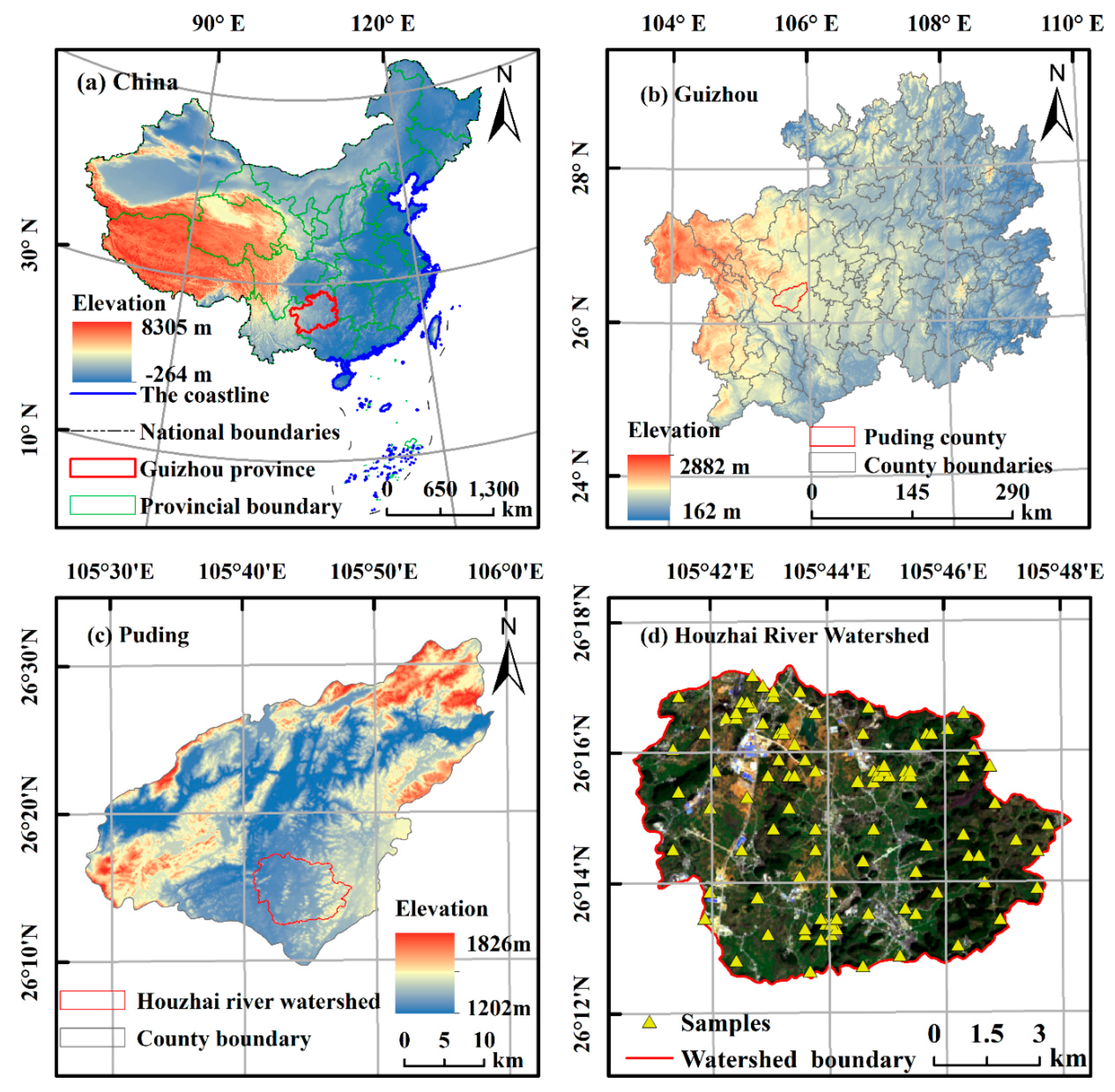
2.1. Study Area and Soil Samples

The Houzhai River Watershed, with a total area of 75 km2, is located in Puding County, Guizhou Province. The terrain is high in the southeast and low in the northwest of the watershed. The highest elevation is 1560 m, and the lowest elevation is 1220 m. Triassic carbonate rocks and karst landforms are widely distributed. The types of land use are diverse, mainly forestland in the upstream and farmland in middle and lower reaches. The spatial distribution pattern of soil is complex and includes limestone soil, paddy soil, and yellow soil.
Sample points are set in accordance with the grid method based on the ArcGIS software (10.2, Environmental Systems Research Institute, Redlands, CA, USA). In actual sampling, the sample information is recorded if samples cannot be collected, and it is replenished and collected nearby based on actual and topographical features. A total of 98 topsoil (0–20 cm) samples were collected and weighed to approximately 1 kg (Figure 1).

2.2. Measurement and Analysis of Metal Contents in Soil

After the soil samples were naturally air dried, decontaminated, ground, and passed through a 200-mesh nylon screen, each sample was divided into two parts, that is, one for chemical analysis and the other for spectral analysis.
The soil sample was subjected to microwave digestion in several steps of hydrochloric acid, nitric acid, hydrofluoric acid, and perchloric acid, and the metal content was determined by four-stage rod-type inductively-coupled plasma mass spectrometry (Q-ICP-MS, PerkinElmer, Canada). Quality control was conducted using the national standard sample GSB04-1767-2004 to ensure the quality of the analysis. Determination of soil organic matter content was performed by the potassium dichromate oxidation external heating method. Descriptive statistical analysis of conventional indicators, such as maximum (Max), minimum (Min), mean, standard deviation (Stdev), and coefficient of variation (CV), for soil metal content was performed in Excel, correlation analysis was performed in SPSS 19.0 (International Business Machines Corporation, Armonk, NY, USA), visualization of correlation coefficient (R) based on RStudio (Auckland University, New Zealand), and kriging interpolation was conducted using the spatial analysis tool of ArcGIS 10.2.

2.3. Soil Spectrometry and Data Pre-Processing

Using a UV–VIS–NIR spectrophotometer by Agilent Technologies to obtain soil sample spectra. The spectral reflectance of 98 samples was measured indoors with a band range of 500–2500 nm and a sampling interval of 1 nm. Three spectral curves were collected for each soil sample and used as the original reflectance spectra after the arithmetic mean.
In the spectral measurement process, it is easy to be affected by random factors and cause errors. The corresponding pre-processing of samples can effectively eliminate the “burr”, enhancing the effective spectral information, and reducing the computational amount to improve the prediction accuracy [40]. Common pre-processing methods include outlier removal, noise reduction, smoothing, and resampling. In this study, standard values (Z-score) and principal component analysis (PCA) were combined to remove the abnormal values and ensure the accuracy of the samples. The median filter and Savitzky–Golay smoothing were combined to reduce and smooth the noise of the spectral data. Then, the spectral data was resampled at an interval of 10 nm, which was regarded as the basis for transformation.
The original spectral reflectance can be transformed in different forms to eliminate noise, purify spectral information, and reduce error. To some extent, it can eliminate spectral translation caused by moisture absorption, amplify spectral information, improve the collimation between spectral data, prevent overfitting, and improve the stability of the model. Common transformation forms include continuum removal, spectral derivative transformation, absorbance transformation, multiple scattering correction (MSC), and standard normal variable (SNV) [41,42]. In our study, transformation included the first derivative of reflectance (RFD), the second derivative of reflectance (RSD), absorbance (AB), the first derivative of absorbance (AFD), the second derivative of absorbance (ASD), MSC, and SNV.
Z-score was performed in SPSS 19.0, and AB and derivative transformations were conducted in Matlab 2016a (MathWorks, Natick, Massachusetts, USA). Others approaches were carried out in The Unscrambler X 10.4 (Camo, Norway).

2.4. Model Establishment and Accuracy Verification

Pearson correlation analysis was performed to analyze the correlation between the variables after re-sampling (OR), RFD, RSD, AB, AFD, ASD, MSC, SNV, and metal contents. The band corresponding to the correlation coefficient with the largest absolute value was the characteristic band. The BP and the GAACA-BP models were established by determining the spectral values corresponding to the characteristic bands as input variables and the soil metal content as output variables. Correlation analysis was conducted in SPSS 19.0, and the models were established in Matlab 2016a by writing a program.

2.4.1. SPXY Sample Division Method

Samples should be divided into calibration and validation sets to verify the stability and reliability of the model. Sample set partitioning based on joint x-y distance (SPXY) sample division method is developed from the Kennard–Stone (KS) method, but the KS method considers x variables only. By contrast, the developed method simultaneously considers x and y variables, thereby effectively covering a multi-dimensional vector space and improving the predictive ability of the established model [43]. Therefore, the SPXY method was used in our study to divide samples. Among them, 69 calibration sets accounted for 75% of the total samples, and 23 validation sets corresponded to 25% of the total samples.

2.4.2. Establishment of the BP Model

A BP model is the most representative of various neural network models. It has a high fault tolerance, and has strong abilities in terms of nonlinear processing, anti-interference, and anti-noise. It is a nonlinear multivariate modelling method widely used in soil hyperspectral quantitative analysis [44,45,46,47]. A three-layer network structure was used to construct the BP model with an output node of 8, an input node of 1, a number of neurons in the hidden layer of 10, and a learning rate of 0.01.

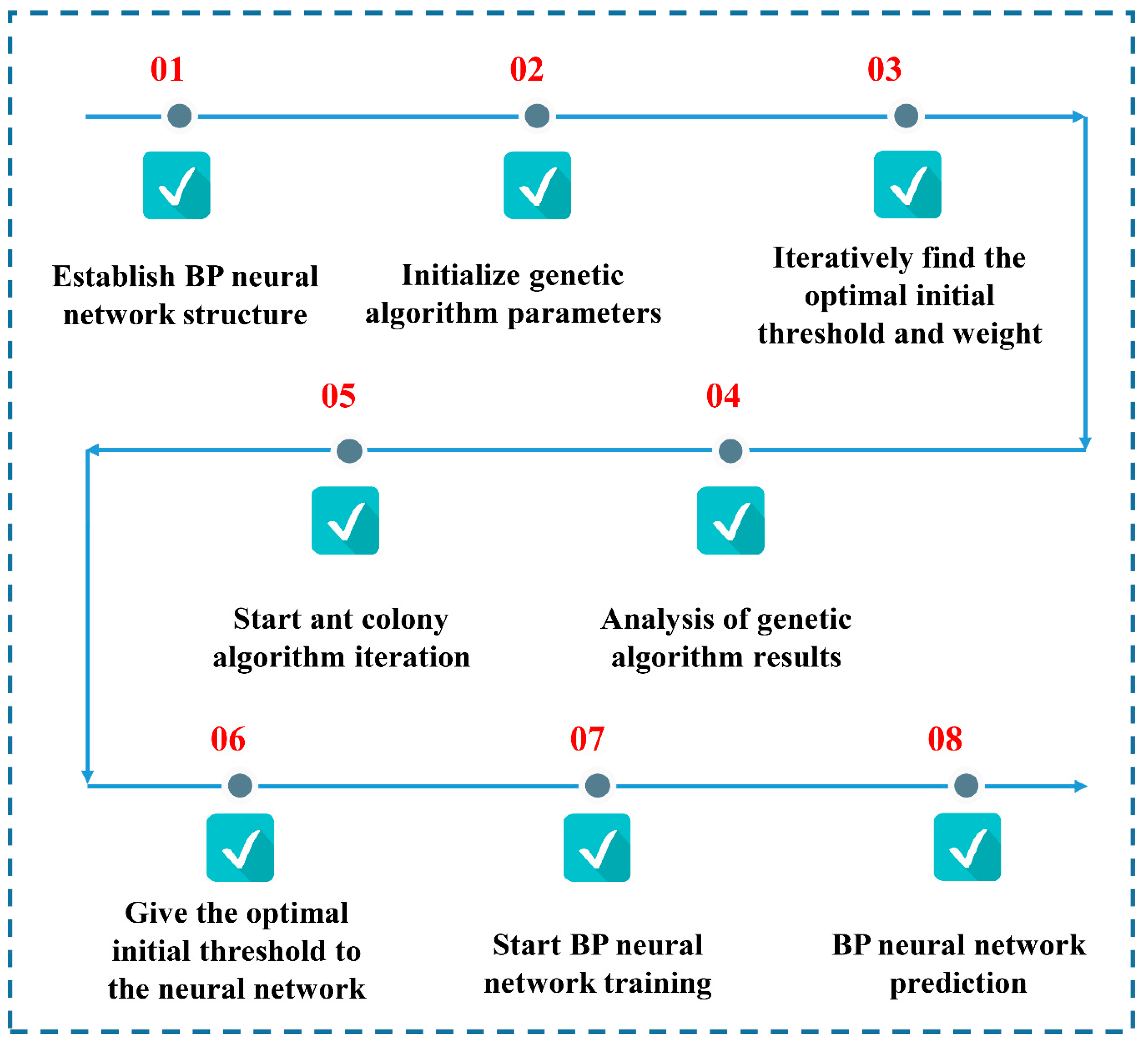
2.4.3. Establishment of the GAACA-BP Model

The ant colony algorithm (ACA) combines distributed computing, positive feedback mechanisms, and greedy search [48], resulting in a strong degree of parallelism and robustness in searching for enhanced solutions, and which is easily integrated with other optimization algorithms. However, ACA requires a long search time and is prone to prematurity and stagnation in solving large optimization problems. GA is a global optimization search method based on random iterative evolution of probabilistic significance, which has wide applicability [49]. It can be used for a global rapid search, but it fails to utilize feedback information in systems effectively, often leading to redundant iterations and low solving efficiency [50]. To overcome the defects of the two algorithms, we merged them to optimize and improve the BP model, and a GAACA-BP model is established. At the early stage, the characteristics of faster convergence and cross-variation operation of GA were used to avoid falling into a local optimum, accelerate the convergence rate of ACA, and improve the efficiency of the solution. In this way, the improved model has the advantages of GA, ACA, and neural networks [51,52]. The implementation of the GAACA-BP model is shown in Figure 2.

2.4.4. Accuracy Verification of the Model

The model results are evaluated by R and the root mean square error (RMSE) of the measured value and the predicted value. The closer R is to 1, the better the prediction effect, the smaller the RMSE, and the better the stability of the model. The prediction ability of the model is expressed by the MRE. The smaller the MRE is, the stronger the prediction ability of the model will be. Conversely, the larger the MRE is, the weaker the prediction ability of the model will be. The formula for calculating the MRE is as follows:
M R E = 1 n i = 1 n | Y m Y P Y m | × 100 %
where Yp is the predicted value, Ym is the measured value, and n is the number of samples.

3. Results

3.1. Analysis of the Metal Content of Soil

3.1.1. Analysis of the Statistical Characteristics of Soil Metal Content

The contents of the four soil metals were measured through ICP-MS, and the results are shown in Table 1. The four metal contents were more than one time higher than the background value based on the background value of the soil average of the A layer in Guizhou Province [53]. In particular, the over-standard rates of Sb and Pb reached 86% and 56%, and the accumulation degree in the soil of the study area was much faster than Cr and Co. This indicates that there is exogenous input of metal content in soil, and Sb and Pb are more affected by human activities.
The CV reflects the relative variability of each variable. Table 1 also shows that the degree of variation of the four metals in the study area from large to small is Sb > Pb > Co > Cr. Among them, Sb has the highest CV of 0.81, and Pb has a CV of 0.61, which is second only to Sb, indicating that the distribution of these two metals is uneven, and the dispersion is large, which may be controlled by human factors. The two other metals have smaller CV values than the first two, suggesting that they are relatively lightly mutated and that the spatial differentiation is relatively small. This result is consistent with the conclusion of the previous paragraph.
The R between metals can explain the similarity of source pathways. The higher R is, the stronger the dependence relationship between metals and the more similar the source will be. On the contrary, the lower R is, the weaker the dependence relationship between metals and the more diverse the source pathways will be. In Table 1, four heavy metals are significantly positively correlated at the 0.01 level, which may suggest that similar sources exist in the study area to control the content and distribution characteristics of heavy metal elements in the soil [54,55].

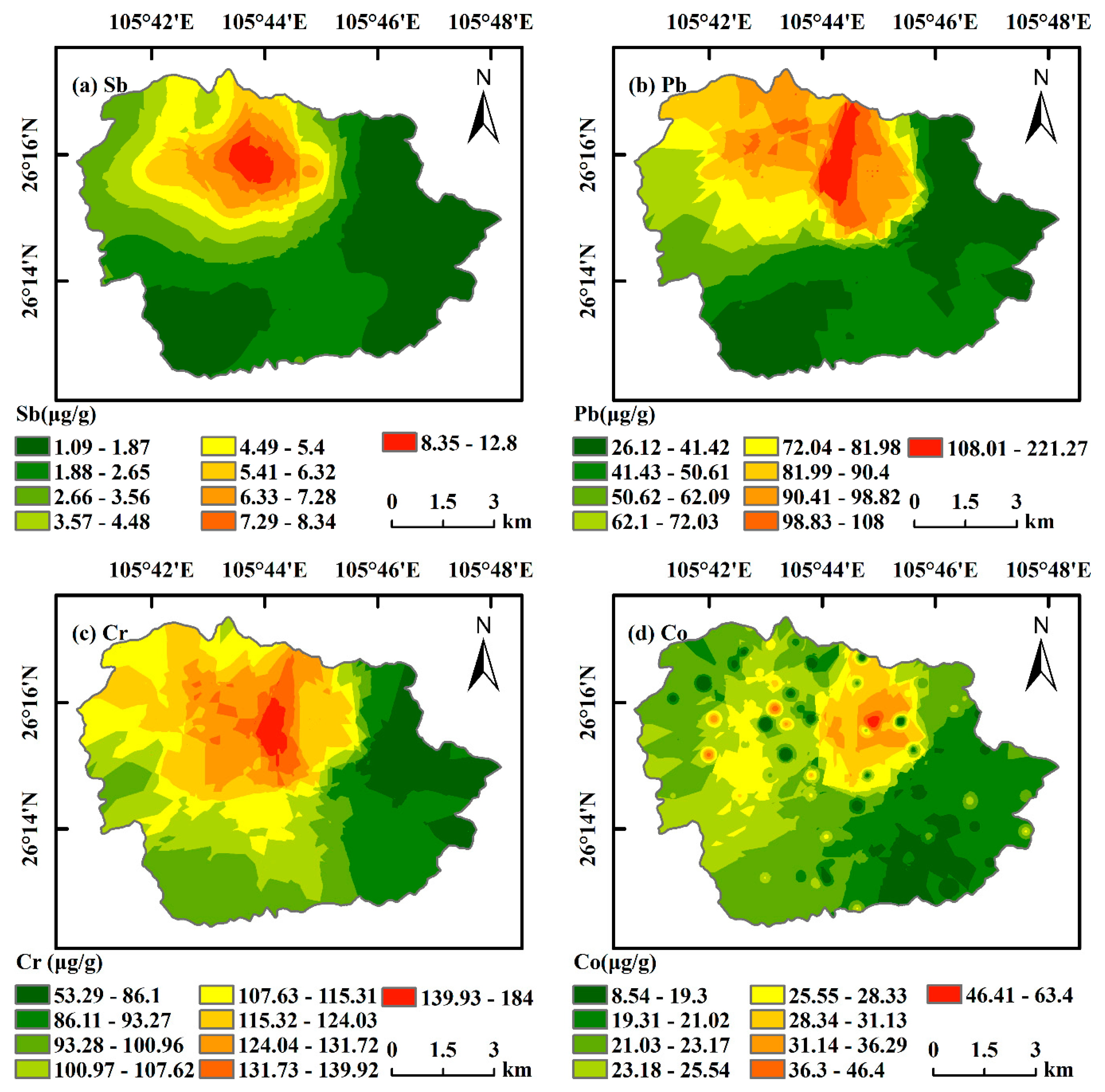
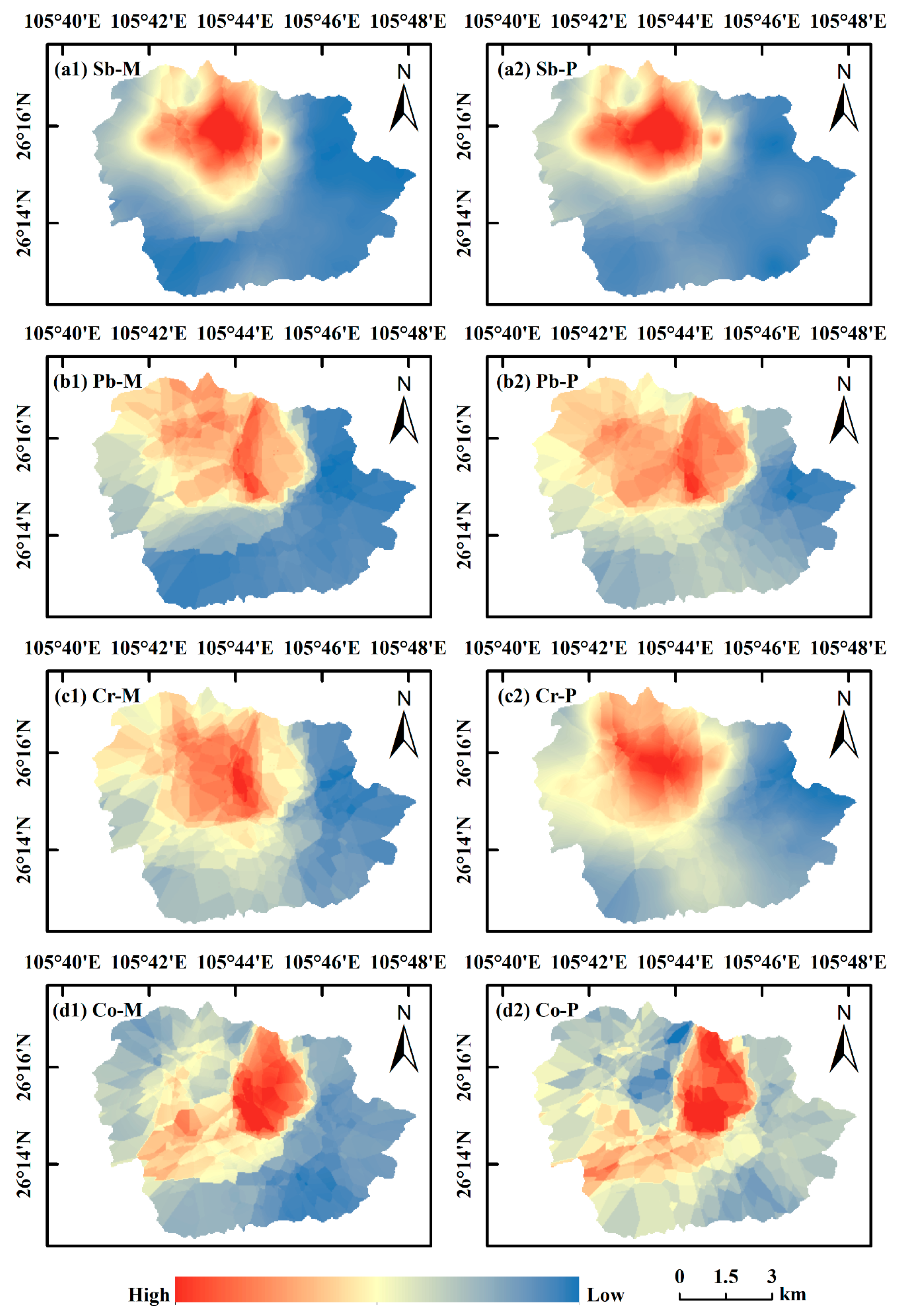
3.1.2. Analysis of the Spatial Distribution Characteristics of Soil Metal Content

The spatial distribution of the metal content in the study area was obtained by using the interpolation tool of the ArcGIS platform to perform ordinary kriging interpolation on the four metal contents (Figure 3). The contents of the four metals are high in the north and low in the south. The spatial distribution patterns of Sb, Pb, and Cr are similar, and the high-value areas are mainly concentrated near Qingshan Reservoir. Sb exhibits a high distribution in the northwest and a relatively low distribution in the southwest and the east. The Sb content decreases from the high-value center to the periphery. Pb is similar to Sb, in particular, high-value areas appear in the north, and relatively low-value areas are in the southwest and the northeast. Cr also has a high value in the north and a low value in the northeast. Different from the first three metals, the distribution of Co is relatively scattered, with multiple islands and block distributions. It may be because the local area is affected by human interference is more intense, but the interference area is small. The high-value area appears in the northeast, the value in the southeast is relatively low. The distribution area in the high-value area is relatively small, and the Co content in most areas is between 8.54 and 23.17 μg/g.

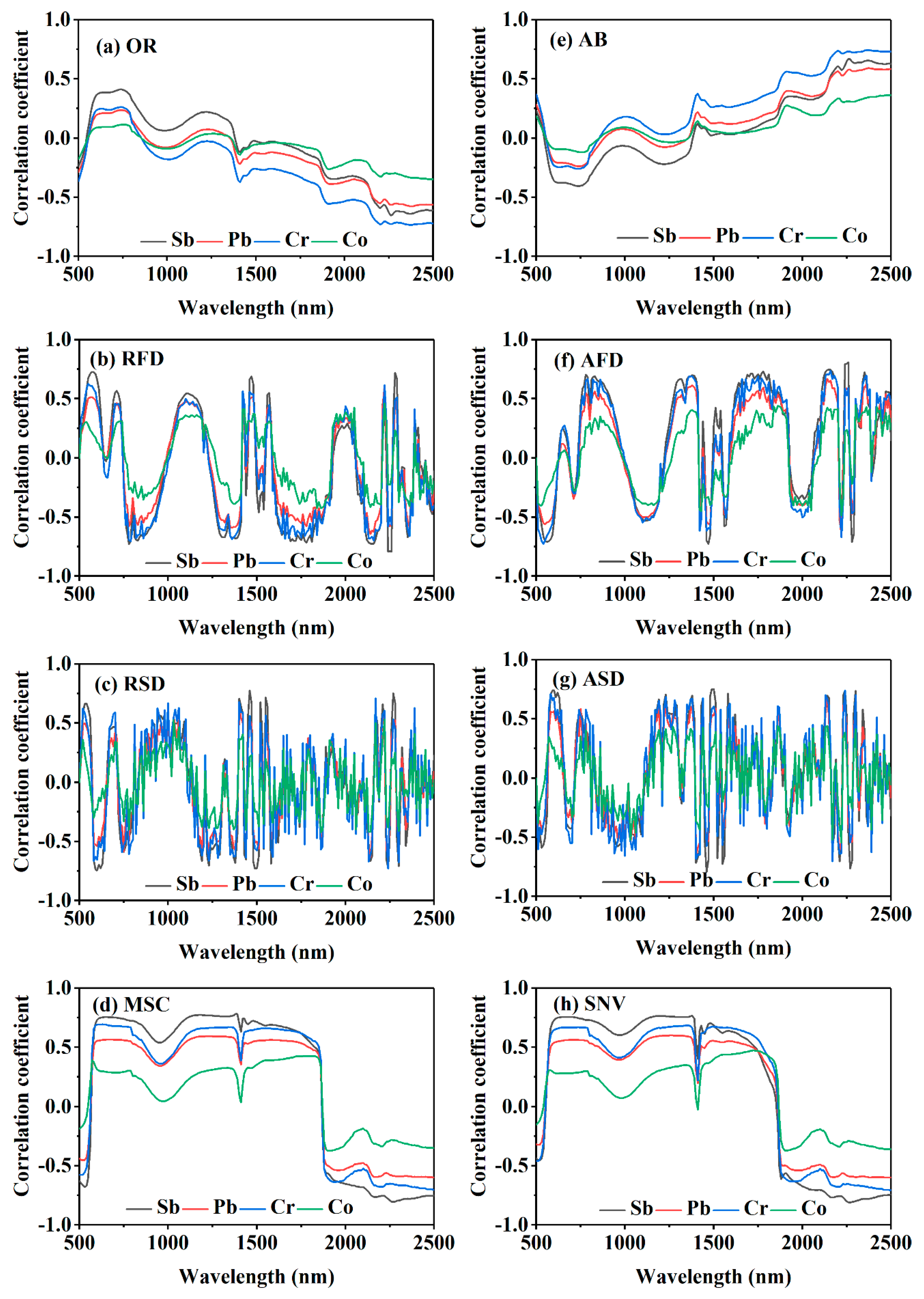
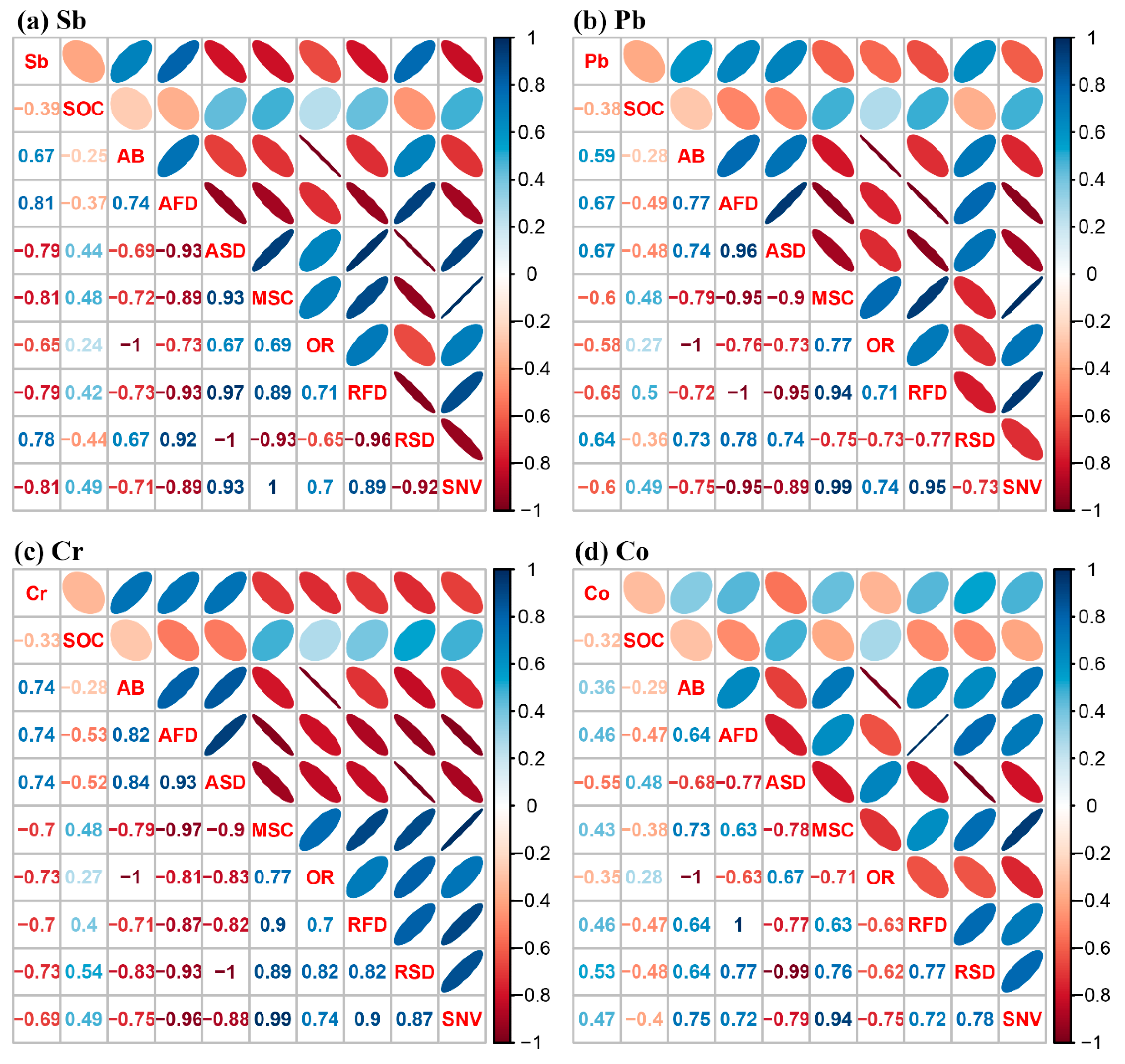
3.2. Screening of Metal Feature Bands

The contents of Sb, Pb, Co, and Cr in soils and the spectral variables were subjected to Pearson correlation analysis, and plotted correlation curves (Figure 4). The trajectories of the correlation curves between the four metals and the spectral variables are substantially the same. The correlation curves of OR and AB are opposite, and the trends of RFD and AFD, RSD and ASD, and MSC and SNV are similar. The four metals were sensitive to the response at the near-infrared band, especially at 2140, 2220, 2260, 2380, and 2500 nm. The correlation between the transformed spectral variables and the metal contents were significantly enhanced (Figure 5). At the 0.01 level, the metal content was significantly negatively correlated with OR and significantly positively correlated with AB and AFD. The correlation of Sb was more significant than that of the three other elements. After SNV transformation was performed, R of Sb reached −0.812 at 2270 nm. Cr was next, and the maximum R was 0.743 at the band of 2380 nm after AB transformation. The maximum R of Pb is 0.669 at the band of 2140 nm after AFD transformation. Co had the lowest correlation, and the maximum R was only −0.547 at the band of 2220 nm after ASD transformation. Each transform filters out an R with the largest absolute value. The corresponding band is the feature band, and the spectral value of each feature band is considered as the input data of the model.
Studies have shown that metals that enter the soil through exogenous sources can be adsorbed by clay minerals, SOC, iron oxides, etc., in the soil, and these key parameters of the soil have typical spectral characteristics. Therefore, bands with significant correlations with these parameters can better predict the metal content of the soil [56]. Pearson correlation analysis was performed between SOC and metal content and the previously selected feature bands (Figure 5). The results show that at the 0.01 level, and all three are significantly correlated, that is, the selected bands can meet the requirements for predicting heavy metal content.

3.3. Hyperspectral Prediction Model of Soil Metal Contents and Accuracy Verification

SPXY sample partition method is used to divide the 92 soil samples of four metals into calibration and validation sets (Figure 6). The calibration set accounted for 3/4 and the validation set accounted for 1/4. The BP and GAACA-BP models were established by considering spectral variables as input data and metal content as output data, respectively.

3.3.1. BP Model Establishment and Verification

In the results of the BP model (Table 2), the R of the calibration sets of the three metal contents, except Co, was greater than 0.5, satisfying the accuracy requirements. The best modelling results are observed in Sb where the R and RMSE reach the maximum and minimum, respectively. R is as high as 0.89, and RMSE is only 2.82. The worst modelling results are detected in Co, where R and RMSE were 0.44 and 28.89, respectively. On the contrary, the fitting effect of the validation set of the four metals is less than 0.5, which fails to pass the precision verification. The worst effect is still observed in Co, whose R and RMSE are 0.19 and 14.82, respectively. The validation set of Sb with the best effect on the calibration set is not as good as expected, R is 0.21, and the RMSE is 1.40. The result is only higher than that of Co. Thus, the traditional BP model is unstable, and an overfitting phenomenon exists possibly because of too much learning that causes the noise in the prediction model to obliterate useful information, resulting in poor generalization.

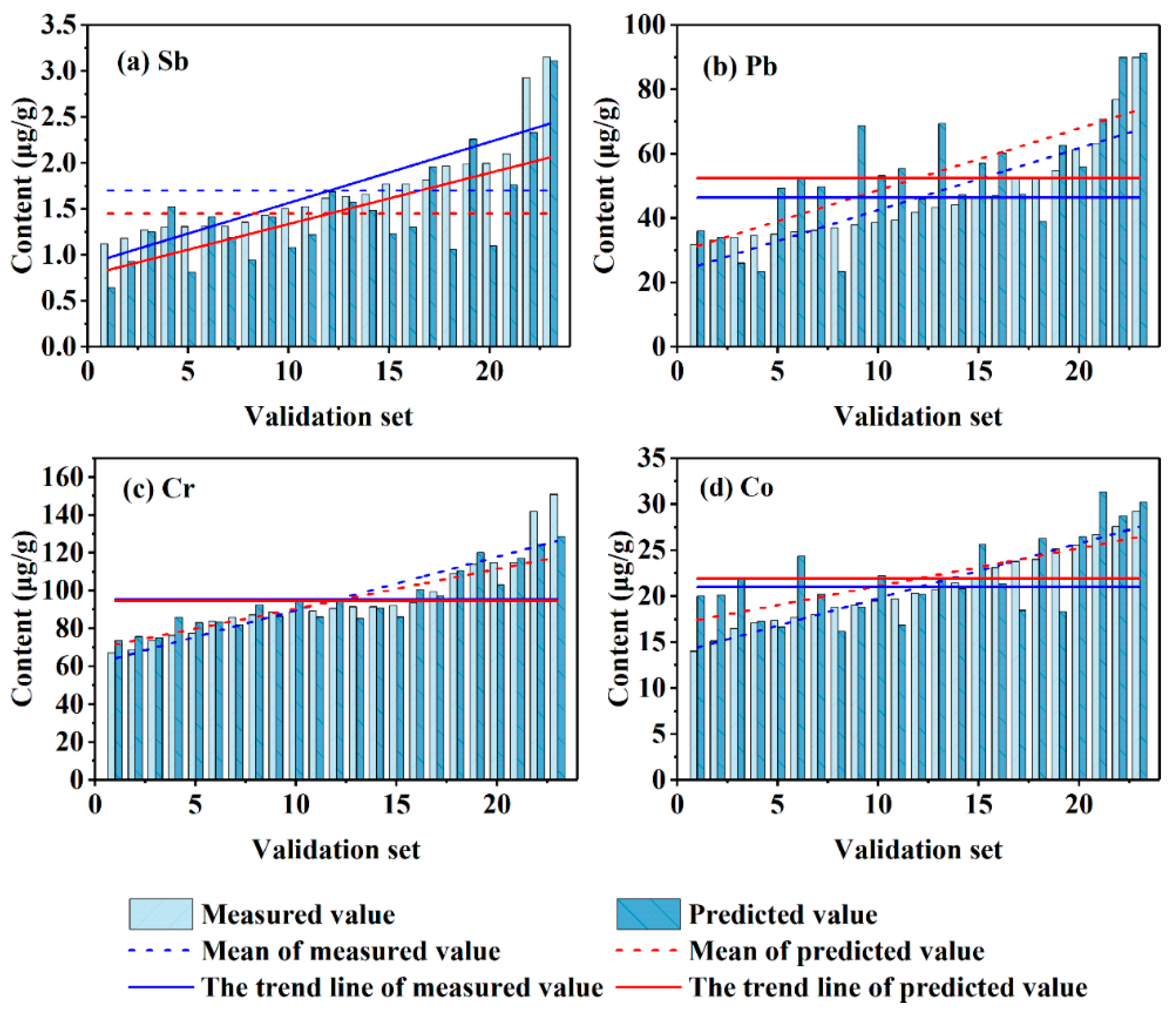
3.3.2. GAACA-BP Model Establishment and Verification

The GAACA is used to improve the BP model, and a new GAACA-BP model is established. As results show in Table 2, the R of the four metals is greater than 0.5, indicating that the model is reliable and can be used to estimate the metal content. In the calibration set, the best effect is that of Sb, with the maximum R of 0.92 and the minimum RMSE value of 0.41. Cr is also effective, with R and RMSE of 0.80 and 31.02, respectively. Pb and Co are slightly less effective, but R is also greater than 0.7. In the validation set, Cr has the best fitting effect with an R of 0.94 and RMSE of 7.91. The second is Sb, whose R is as high as 0.82 and RMSE is 2.16. Pb has the third effect, while Co is the worst. The R values of both metals is 0.76 and 0.67, respectively. The trend line and mean value are shown that the overall predicted value of Pb and Co is higher than the measured value, whereas the overall predicted value of Sb and Cr is lower than the measured value (Figure 7). In order to further verify the prediction effect of the GAACA-BP model, this paper uses the same method and parameters to interpolate the measured and predicted values based on the Arc GIS platform. As shown in Figure 8, the spatial distribution characteristics of the measured values and predicted values of the four metals are basically the same, especially in the high value region. Moreover, the larger the R, the smaller the difference in the spatial distribution of the metals. From the perspective of space, Sb and Cr are underestimated, while Pb and Co are overestimated, which is consistent with the research results in Figure 6.
The fitting effect and stability of the new GAACA-BP model are greatly improved compared with that of the BP model (Table 3). The improvement of the calibration set was relatively smaller than that of the validation set, where the most significant increase in R of Co is from 0.44 to 0.79 (34%). In contrast to the validation set, the calibration set of the prediction accuracy of the metals is greatly improved, and R is increased by more than 48% compared with that of the original BP model. The change in Sb is the most significant, and R of the validation set increases from 0.21 to 0.82, indicating an increase of 61%. In summary, the adaptability of the GAACA-BP model from large to small is Sb > Cr > Pb > Co.

4. Discussion

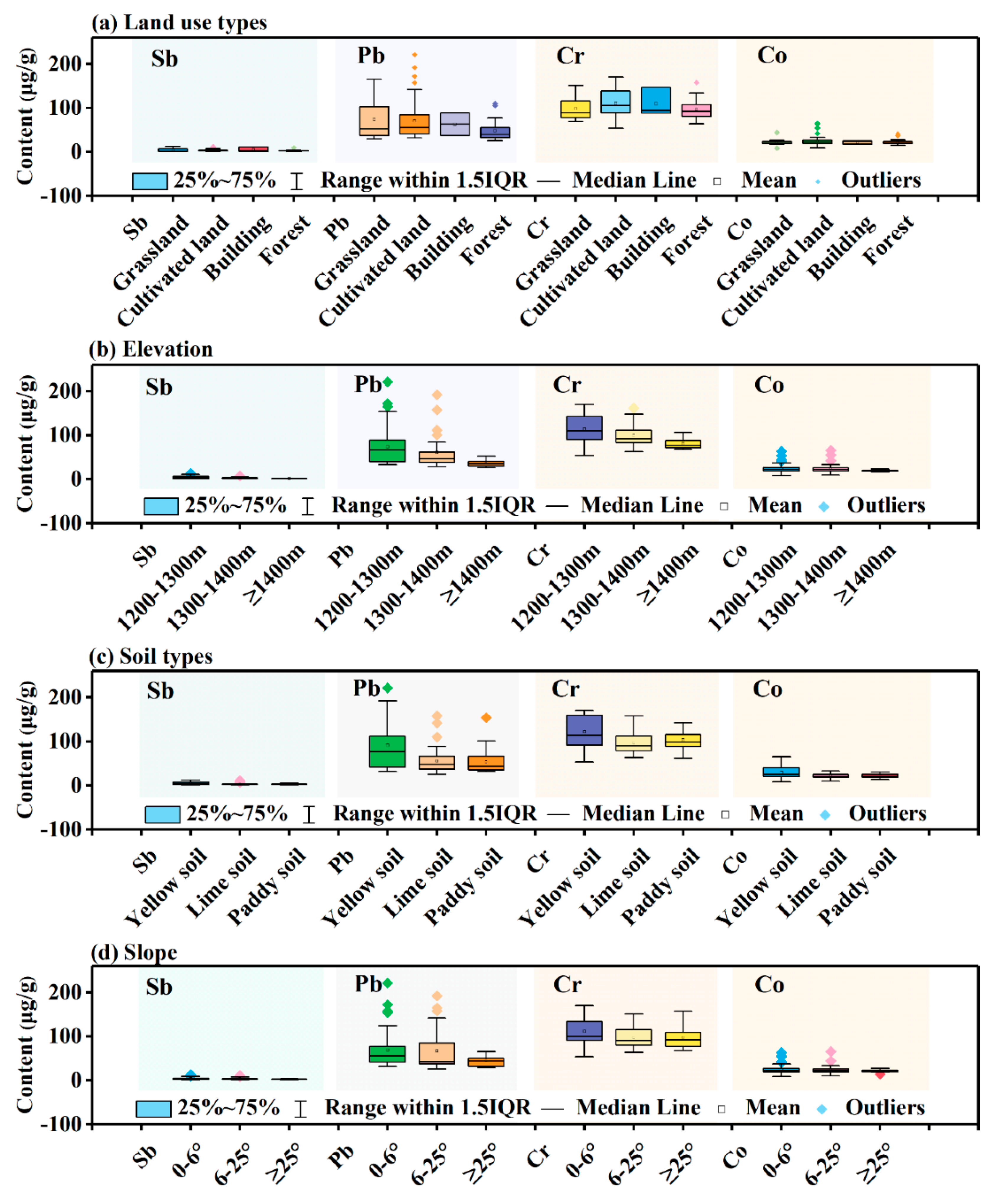
4.1. Factors Affecting the Distribution of the Metal Content

Different geographical factors, especially land use patterns, have various effects on the accumulation of metal elements [57,58,59,60,61]. The soil metals in the study area have different degrees of accumulation under various land use patterns, elevations, soil types, and slopes, but the cumulative characteristics are generally consistent (Figure 9). From the perspective of land use, the average content of Sb from high to low is building > grassland > cultivated land > forest. The average content of Pb is grassland > cultivated land > building > forest. The average content of Cr is cultivated land > building > grassland > forest. The average content of Co is cultivated land > forest > building > grassland. The four metal elements are generally higher in cultivated land and lower in forest, indicating that the accumulation of metals in soil may be caused by the application of agricultural materials, such as fertilizers, organic fertilizers, and pesticides in agricultural activities. From the elevation point of view, except for the content of Co, which is medium elevation (1300–1400 m) > low elevation (1200–1300 m) > high elevation (≥1400 m), the other three metals are higher in elevation and lower in content. This shows that the lower the elevation, the greater the possibility of metal accumulation; From the soil type, the contents of Sb and Pb are yellow soil > lime soil > paddy soil, and the contents of Cr and Co are yellow soil > paddy soil > lime soil. It can be seen that high concentrations of metals tend to accumulate in yellow soil; From the aspect of slope, except for the content of Cr being flat slope (0–6°) > steep slope (≥25°) > gentle slope (6–25°), the accumulation characteristics of the other three metals are more pronounced where the slope is smaller. Thus, the metals in soil easily accumulate in the region with small topographic fluctuations and a flat terrain.
In summary, the metals in the soil in the study area are greatly affected by human activities, especially agricultural activities, and the migration process of the metals in the soil in the study area is speculated on the basis of the following: soil metals enter the soil with the input of different types of agricultural materials, such as fertilizers and pesticides. Under the action of transportation and accumulation, it gradually accumulates in the middle and lower reaches of the watershed with a relatively low altitude, small slope, flat topography, and extensive yellow soil areas.

4.2. Prediction Capability Analysis of the GAACA-BP Model

MRE is often used to evaluate the predictive ability of the model. The smaller the MRE is, the stronger the prediction ability of the model will be [62,63,64]. In Table 4, the MRE of the original BP model of four metals (Sb, Pb, Cr, and Co) is between 21% and 79%, with Sb as the largest and Cr as the smallest. The MRE of the GAACA-BP model improved by GAACA is greatly reduced, and the range of MRE is 6%–15%. Therefore, the prediction accuracy of the model is between 85% and 94%. The error is reduced by 12–64 percentage points, that is to say, the accuracy is improved by 12–64 percentage points. The most significant improvement is observed in the Sb content predicted by the GAACA-BP model, and the accuracy is increased from 21% to 85% (64%). Although the ability of the model to predict the Cr content is the least significant, the accuracy increases from 79% to 91%, which corresponds to an increase of 12%. In summary, the prediction ability of the GAACA-BP model for different metals from high to low is Cr > Co > Sb > Pb.
In the past, a large number of surveys on soil were carried out around the world, such as the Forum of European Geological Surveys (FOREGS), The Geochemical Mapping of Agricultural and Grazing Land Soil in Europe (GEMAS), and Eurostat Land Use/Land Cover Area frame Survey (LUCAS). A large number of soil samples were collected. Based on this, many scholars have simulated the spatial distribution of soil metals and obtained reliable results [65,66]. For example, Lado et al. used the geostatistical method to simulate the distribution of eight metals including Pb and Cr in the topsoil based on the FOREGS Geochemical database. The spatial distribution map was drawn using the regression regression-kriging method, and a large number of raster maps were used to improve the prediction [67]. Although the results of this study are satisfactory, compared to hyperspectral models, this traditional method requires more cost to perform large-scale sampling, and improved prediction also requires more data support. Comparing Table 5, the prediction effect of the traditional method is not necessarily better than the hyperspectral model. The hyperspectral model is relatively simple, convenient, low-cost, and more applicable.
At present, the researches on hyperspectral variable prediction of metal content are mostly based on linear model, while the researches on nonlinear model including neural network are relatively rare. Among the four metals studied in this paper, the spectral prediction studies of Sb and Co are also rare for Pb and Cr. Therefore, this paper makes a simple comparison between the results of the prediction of Pb, Cr by linear or nonlinear models and the results of this paper. It can be seen from Table 5 that whether it is Cr or Pb, this paper can achieve a better effect than other studies, especially the prediction effect of GAACA-BP on Cr. At the same time, it can be found from the comparison that the prediction accuracy of the nonlinear model seems to be generally better than the linear model. Of course, the accumulation of heavy metals is affected by many factors. In this paper, only a small part of the literature is selected as a comparative analysis. Whether this discovery is universal or not, further research is needed in future studies.

4.3. Insufficient and Prospects of Research

The small watershed of a typical karst plateau in Guizhou is selected as the study area. The statistical and spatial distribution characteristics of four metals (Sb, Pb, Cr, and Co) in the soil are analyzed. An original BP metal content prediction model is constructed on the basis of hyperspectral data, and the model is improved on the basis of GAACA. The results confirm that the improved GAACA-BP model is more stable and reliable. This finding not only has a practical value for the monitoring of soil metal pollution in the watershed but also has a certain reference value for other similar studies. However, the research still has the following shortcomings:
Although the spatial distribution characteristics and possible influencing factors of the four soil metals in the study area are analyzed, the internal migration mechanism is not examined in depth.
The model itself has certain limitations. On the one hand, using Matlab for programming is difficult. On the other hand, the influencing factors of soil metal contents are different because of various regions. The applicability of the model in different regions or geographical backgrounds remains to be verified.
Limitations of indoor hyperspectral. Although indoor spectroscopy requires much less time and labor compared with traditional methods, a smaller amount of field sampling is necessary compared with that of satellite-borne or aircraft-mounted hyperspectral images. Indoor spectroscopy may be subject to the limitations of equipment and cause measurement errors.
In future research, the factors affecting the accumulation of metals will be further analyzed, and hyperspectral imagery carried by satellite or aircraft will be used. Combined with the characteristics of karst area, geographical factors will be used as variable factors to further improve the prediction model. Isotopes can also be used to investigate the effects of metal accumulation in soil on human health.

5. Conclusions

Sb, Pb, Cr, and Co have different degrees of accumulation in the soil in the study area. Among them, the accumulation of Pb is the most serious, followed by Sb. The spatial differentiation characteristics and dispersion of these two metals are more significant than that of Cr and Co. The four heavy metal elements show a significantly positive correlation at the 0.01 level, indicating that they may have similar source pathways, but the degree of impact is slightly different.
The spatial distribution of the four metals is generally high in the north and low in the south. The regularity of Sb, Pb, and Cr is evident and similar. The high-value area appears near the Qingshan Reservoir and decreases from the high-value center to the periphery. The east is relatively lower than the southwest. The spatial distribution of Co is relatively scattered, and it is distributed in a combination of multiple islands and blocks. Moreover, these four metals in the study area are likely interfered by human factors, especially agricultural activities, and are highly accumulated in a cultivated land with a relatively low elevation, flat terrain, and wide distribution of yellow soil.
The prediction model of soil metal content established by the BP neural network has a good modelling effect but the prediction effect is not ideal. The MRE is larger, between 21% and 79%, and the R value is less than 0.5, denoting a failed accuracy verification. Thus, the original BP model is extremely unstable, and an overfitting phenomenon exists.
The GAACA-BP model is greatly improved by the GAACA in terms of the modelling effect and prediction accuracy compared with those of the original BP models. The R and spatial distribution characteristics of measured and predicted values confirm that the model is reliable and can be used to predict the metal content of soil. The prediction accuracy of the improved model is between 85% and 94%, which is 12–64 percentage points higher than that of the original model. Among them, the improvement effect of Sb is the most evident. In general, the prediction ability of the GAACA-BP model for different elements from strong to weak is Cr > Co > Sb > Pb.

Author Contributions

Conceptualization: S.W., X.B., D.Z., and G.L.; data curation: S.T., J.W., M.W., and Q.L.; formal analysis: S.T.; funding acquisition: S.W. and X.B.; investigation: S.T., J.W., M.W., and Q.L.; methodology: S.T., S.W., X.B., D.Z., and G.L.; project administration: S.W. and X.B.; resources: S.W. and X.B.; supervision: D.Z. and G.L.; validation: S.T., Y.Y., Z.H., C.L., and Y.D.; writing—original draft: S.T.; writing—review and editing: Y.Y. and Z.H.

Funding

This research was funded by National Key Research Program of China (nos. 2016YFC0502102 and 2016YFC0502300), “Western light” Talent Training Plan (Class A), Chinese Academy of Science And Technology Services Network Program (no. KFJ-STS-ZDTP-036), the International Cooperation Agency International Partnership Program (no. 132852KYSB20170029, no. 2014-3), the Guizhou High-Level Innovative Talent Training Program “Ten” Level Talents Program (no. 2016-5648), the United Fund of Karst Science Research Center (no. U1612441), International Cooperation Research Projects of the National Natural Science Fund Committee (nos. 41571130074 and 41571130042), and the Science and Technology Plan of Guizhou Province of China (no. 2017-2966).

Conflicts of Interest

The author(s) declared no potential conflicts of interest with respect to the research, authorship, and/or publication of this article.

References

  1. Tengbing, H.E.; Lingling, D.O.N.G.; Guangzhi, L.I.; Yuansheng, L.I.U.; Yingge, S.H.U.; Haibo, L.U.O.; Fang, L.I.U. Differences of Heavy Metal Contents in Soils Derived from Different Parent Materials/Rocks in Karst Mountain Area. J. Agro Environ. Sci. 2008, 27, 188–193. [Google Scholar]
  2. Zhang, D.; Zhou, M.Z.; Xiong, K.N.; Gu, B.Q.; Yang, H. Risk Assessment of Copper and Zinc in Soils and Crops around the Ni-Mo Mining Area of Songlin, Zunyi, China. Earth Environ. 2019, 38, 356–365. [Google Scholar]
  3. Galán, E.; Romero-Baena, A.J.; Aparicio, P.; González, I. A methodological approach for the evaluation of soil pollution by potentially toxic trace elements. J. Geochem. Explor. 2019, 4, 5. [Google Scholar]
  4. Obeng-Gyasi, E. Sources of lead exposure in various countries. Rev. Environ. Health 2019, 34, 25–34. [Google Scholar] [CrossRef] [PubMed]
  5. He, M.C.; Wan, H.Y. Distribution, speciation, toxicity and bioavailability of antimony in the environment. Prog. Chem. Beijing 2004, 16, 131–135. [Google Scholar]
  6. ATSDR (Agency for Toxic Substances and Disease Registry). Toxicological Profile. Available online: https://www.atsdr.cdc.gov/toxprofiledocs/index.html (accessed on 4 January 2019).
  7. Gebel, T.; Christensen, S.; Dunkelberg, H. Comparative and environmental genotoxicity of antimony and arsenic. Anticancer Res. 1997, 17, 2603. [Google Scholar] [PubMed]
  8. Chen, X.D.; Lu, X.W.; Zhao, C.F.; Luo, D.C. The Spatial Distribution of Heavy Metals in the Urban Topsoil Collected from the Interior Area of the Second Ring Road, Xi’an. Acta Geogr. Sin. 2011, 66, 1281–1288. [Google Scholar]
  9. Jiang, Y.; Chao, S.; Liu, J.; Yang, Y.; Chen, Y.; Zhang, A.; Cao, H. Source apportionment and health risk assessment of heavy metals in soil for a township in Jiangsu Province, China. Chemosphere 2016, 168, 1658–1668. [Google Scholar] [CrossRef] [PubMed]
  10. Guan, Q.; Wang, F.; Xu, C.; Pan, N.; Lin, J.; Zhao, R.; Luo, H. Source apportionment of heavy metals in agricultural soil based on PMF: A case study in Hexi Corridor, northwest China. Chemosphere 2017, 193, 189–197. [Google Scholar] [CrossRef] [PubMed]
  11. Hu, H.; Téllez-Rojo, M.M.; Bellinger, D.; Smith, D.; Ettinger, A.S.; Lamadrid-Figueroa, H.; Hernández-Avila, M. Fetal lead exposure at each stage of pregnancy as a predictor of infant mental development. Environ. Health Perspect. 2006, 114, 1730–1735. [Google Scholar] [CrossRef] [PubMed]
  12. Reuben, A.; Caspi, A.; Belsky, D.W.; Broadbent, J.; Harrington, H.; Sugden, K.; Moffitt, T.E. Association of Childhood Blood Lead Levels With Cognitive Function and Socioeconomic Status at Age 38 Years and With IQ Change and Socioeconomic Mobility Between Childhood and Adulthood. JAMA 2017, 317, 1244–1251. [Google Scholar] [CrossRef] [PubMed]
  13. Lanphear, B.P.; Rauch, S.; Auinger, P.; Allen, R.W.; Hornung, R.W. Low-level lead exposure and mortality in US adults: A population-based cohort study. Lancet Public Health 2018, 3, e177–e184. [Google Scholar] [CrossRef]
  14. Obeng-Gyasi, E.; Armijos, R.; Weigel, M.; Filippelli, G.; Sayegh, M. Cardiovascular-Related Outcomes in US Adults Exposed to Lead. Int. J. Environ. Res. Public Health 2018, 15, 759. [Google Scholar] [CrossRef] [PubMed]
  15. Harari, F.; Sallsten, G.; Christensson, A.; Petkovic, M.; Hedblad, B.; Forsgard, N.; Barregard, L. Blood Lead Levels and Decreased Kidney Function in a Population-Based Cohort. Am. J. Kidney Dis. 2018, 72, 381–389. [Google Scholar] [CrossRef] [PubMed] [Green Version]
  16. Lin, J.L.; Lin-Tan, D.T.; Hsu, K.H.; Yu, C.C. Environmental Lead Exposure and Progression of Chronic Renal Diseases in Patients without Diabetes. N. Engl. J. Med. 2003, 348, 277–286. [Google Scholar] [CrossRef] [PubMed]
  17. Obeng-Gyasi, E.; Armijos, R.; Weigel, M.; Filippelli, G.; Sayegh, M. Hepatobiliary-Related Outcomes in US Adults Exposed to Lead. Environments 2018, 5, 46. [Google Scholar] [CrossRef]
  18. Can, S.; Bağci, C.; Ozaslan, M.; Bozkurt, A.I.; Cengiz, B.; Cakmak, E.A.; Tarakçioğlu, M. Occupational lead exposure effect on liver functions and biochemical parameters. Acta Physiol. Hung. 2008, 95, 395–403. [Google Scholar] [CrossRef]
  19. Römkens, P.F.A.M.; Guo, H.Y.; Chu, C.L.; Liu, T.S.; Chiang, C.F.; Koopmans, G.F. Enrichment characteristics and risk prediction of heavy metals for rice grains growing in paddy soils with a high geological background. J. Agro Environ. Sci. 2018, 37, 18–26. [Google Scholar]
  20. Ruan, Y.L.; Li, X.D.; Li, T.Y.; Chen, P.; Lian, B. Heavy Metal Pollution in Agricultural Soils of the Karst Areas and Its Harm to Human Health. Earth Environ. 2015, 43, 92–97. [Google Scholar]
  21. Wu, F.; Zheng, J.; Pan, X.; Li, W.; Deng, Q.; Mo, C.; Guo, J.Y. Prospect on Biogeochemical Cycle and Environmental Effect of Antimony. Adv. Earth Sci. 2008, 23, 350–356. [Google Scholar]
  22. Liu, J.; Zhang, Y.; Wang, H.; Du, Y. Study on the prediction of soil heavy metal elements content based on visible near-infrared spectroscopy. Spectrochim. Acta Part A Mol. Biomol. Spectrosc. 2018, 199, 43. [Google Scholar] [CrossRef] [PubMed]
  23. Shi, T.; Chen, Y.; Liu, Y.; Wu, G. Visible and near-infrared reflectance spectroscopy-an alternative for monitoring soil contamination by heavy metals. J. Hazard. Mater. 2014, 265, 166. [Google Scholar] [CrossRef] [PubMed]
  24. Ullah, S.; Skidmore, A.K.; Naeem, M.; Schlerf, M. An accurate retrieval of leaf water content from mid to thermal infrared spectra using continuous wavelet analysis. Sci. Total Environ. 2012, 437, 145–152. [Google Scholar] [CrossRef] [PubMed]
  25. Xu, H.; Qi, B.; Sun, T.; Fu, X.; Ying, Y. Variable selection in visible and near-infrared spectra: Application to on-line determination of sugar content in pears. J. Food Eng. 2012, 109, 142–147. [Google Scholar] [CrossRef]
  26. McCarty, G.W.; Reeves, J.B.; Reeves, V.B.; Follett, R.F.; Kimble, J.M. Mid-Infrared and Near-Infrared Diffuse Reflectance Spectroscopy for Soil Carbon Measurement. Soil Sci. Soc. Am. J. 2002, 66, 640–646. [Google Scholar]
  27. Nocita, M.; Stevens, A.; Toth, G.; van Wesemael, B.; Montanarella, L. Prediction of SOC content by Vis-NIR spectroscopy at European scale using a modified local PLS algorithm. In Proceedings of the AGU Fall Meeting Abstracts, Washington, DC, USA, 30 August 2012. [Google Scholar]
  28. Rossel, R.V.; Walvoort, D.J.J.; McBratney, A.B.; Janik, L.J.; Skjemstad, J.O. Visible, near infrared, mid infrared or combined diffuse reflectance spectroscopy for simultaneous assessment of various soil properties. Geoderma 2006, 131, 59–75. [Google Scholar] [CrossRef]
  29. Dunn, B.W.; Batten, G.D.; Beecher, H.G.; Ciavarella, S. The potential of near-infrared reflectance spectroscopy for soil analysis--a case study from the Riverine Plain of south-eastern Australia. Aust. J. Exp. Agric. 2002, 42, 607–614. [Google Scholar] [CrossRef]
  30. Chakraborty, S.; Li, B.; Deb, S.; Paul, S.; Weindorf, D.C.; Das, B.S. Predicting soil arsenic pools by visible near infrared diffuse reflectance spectroscopy. Geoderma 2017, 296, 30–37. [Google Scholar] [CrossRef]
  31. Sun, W.; Zhang, X. Estimating soil zinc concentrations using reflectance spectroscopy. Int. J. Appl. Earth Obs. Geoinf. 2017, 58, 126–133. [Google Scholar] [CrossRef]
  32. Ng, W.; Malone, B.P.; Minasny, B. Rapid assessment of petroleum-contaminated soils with infrared spectroscopy. Geoderma 2017, 289, 150–160. [Google Scholar] [CrossRef]
  33. Yu, X.; Liu, Q.; Wang, Y.; Liu, X.; Liu, X. Evaluation of MLSR and PLSR for estimating soil element contents using visible/near-infrared spectroscopy in apple orchards on the Jiaodong peninsula. Catena 2016, 137, 340–349. [Google Scholar] [CrossRef]
  34. Bak, J. Retrieving CO Concentrations from FT-IR Spectra with Nonmodeled Interferences and Fluctuating Baselines Using PCR Model Parameters. Appl. Spectrosc. 2001, 55, 591–597. [Google Scholar] [CrossRef]
  35. Pandit, C.M.; Fieippelli, G.M.; Li, L. Estimation of heavy-metal contamination in soil using reflectance spectroscopy and partial least-squares regression. Int. J. Remote Sens. 2010, 31, 4111–4123. [Google Scholar] [CrossRef]
  36. Gholizadeh, A.; Borůvka, L.; Saberioon, M.M.; Kozák, J.; Vašát, R.; Němeček, K. Comparing different data preprocessing methods for monitoring soil heavy metals based on soil spectral features. Soil Water Res. 2015, 10, 218–227. [Google Scholar] [CrossRef]
  37. Ferreira, E.C.; Milori, D.M.; Ferreira, E.J.; Da Silva, R.M.; Martin-Neto, L. Artificial neural network for Cu quantitative determination in soil using a portable Laser Induced Breakdown Spectroscopy system. Spectrochim. Acta Part B At. Spectrosc. 2008, 63, 1216–1220. [Google Scholar] [CrossRef]
  38. Luce, M.S.; Ziadi, N.; Gagnon, B.; Karam, A. Visible near infrared reflectance spectroscopy prediction of soil heavy metal concentrations in paper mill biosolid- and liming by-product-amended agricultural soils. Geoderma 2017, 288, 23–36. [Google Scholar] [CrossRef]
  39. Shi, T.; Wang, J.; Chen, Y.; Wu, G. Improving the prediction of arsenic contents in agricultural soils by combining the reflectance spectroscopy of soils and rice plants. Int. J. Appl. Earth Obs. Geoinf. 2016, 52, 95–103. [Google Scholar] [CrossRef]
  40. Song, L.; Jian, J.; Tan, D.J.; Xie, H.B.; Luo, Z.F.; Gao, B. Estimate of heavy metals in soil and streams using combined geochemistry and field spectroscopy in Wan-sheng mining area, Chongqing, China. Int. J. Appl. Earth Obs. Geoinf. 2015, 34, 1–9. [Google Scholar] [CrossRef]
  41. Chakraborty, S.; Weindorf, D.C.; Paul, S.; Ghosh, B.; Li, B.; Ali, M.N.; Majumdar, K. Diffuse reflectance spectroscopy for monitoring lead in landfill agricultural soils of India. Geoderma Reg. 2015, 5, 77–85. [Google Scholar] [CrossRef]
  42. Cambou, A.; Cardinael, R.; Kouakoua, E.; Villeneuve, M.; Durand, C.; Barthès, B.G. Prediction of soil organic carbon stock using visible and near infrared reflectance spectroscopy (VNIRS) in the field. Geoderma 2016, 261, 151–159. [Google Scholar] [CrossRef] [Green Version]
  43. Galvao, R.K.H.; Araujo, M.C.U.; Jose, G.E.; Pontes, M.J.C.; Silva, E.C.; Saldanha, T.C.B. A method for calibration and validation subset partitioning. Talanta 2005, 67, 736–740. [Google Scholar] [CrossRef] [PubMed]
  44. Zheng, L.H.; Li, M.Z.; Pan, L.; Sun, J.Y.; Tang, N. Estimation of soil organic matter and soil total nitrogen based on NIR spectroscopy and BP neural network. Spectrosc. Spectr. Anal. 2008, 28, 1160–1164. [Google Scholar]
  45. Shen, R.; Ding, G.; Wei, G.; Sun, B. Retrieval of soil organic matter content from hyper-spectrum based on ANN. Acta Pedol. Sin. 2009, 46, 391–397. [Google Scholar]
  46. Lan, Z.Y.; Liu, Y. Research on Indirect Hyperspectral Estimating Model and the Spatial Distribution Characteristics of Heavy Metal Contents in Basin Soil of Lean River. Geogr. Geo Inf. Sci. 2015, 31, 26–32. [Google Scholar]
  47. Liang-ji, X.; Qing-qing, L.; Xiao-mei, Z.; Shu-guang, L. Hyperspectral Inversion of Heavy Metal Content in Coal Gangue Filling Reclamation Land. Spectrosc. Spectr. Anal. 2017, 37, 3839–3844. [Google Scholar]
  48. Dorigo, M.; Stützle, T. Ant Colony Optimization: Overview and Recent Advances. In Handbook of Metaheuristics; Potvin, J.-Y., Gendreau, M., Eds.; Springer: Berlin, Germany, 2010; pp. 227–263. [Google Scholar] [Green Version]
  49. Li, H.M. Overview of Genetic Algorithms. Softw. Guide 2009, 1, 67–68. [Google Scholar]
  50. Cao, Q.K.; Zhao, F. Port trucks route optimization based on GA-ACO. Syst. Eng. Theory Pract. 2013, 33, 1820–1828. [Google Scholar]
  51. Dréo, J.; Siarry, P. Continuous interacting ant colony algorithm based on dense heterarchy. Future Gener. Comput. Syst. 2004, 20, 841–856. [Google Scholar] [CrossRef]
  52. Cao, M.; Huang, Y.F.; Gu, L.Z.; Hu, Z.M.; Yang, Y.X. Construction of S-boxes based on genetic and ant colony algorithm. Appl. Res. Comput. 2008, 25, 1553–1555. [Google Scholar]
  53. China national environmental monitoring Centre. Chinese Soil Element Background Value; China Environmental Science Press: Beijing, China, 1990. [Google Scholar]
  54. Wang, J.; Chen, Z.L.; Wang, C.; Ye, M.W.; Shen, J.; Nie, Z.L. Heavy metal content and ecological risk warning assessment of vegetable soils in Chongming Island, Shanghai City. Environ. Sci. 2007, 28, 647. [Google Scholar]
  55. Sun, Y.; Zhou, Q.; Xie, X.; Liu, R. Spatial, sources and risk assessment of heavy metal contamination of urban soils in typical regions of Shenyang, China. J. Hazard. Mater. 2010, 174, 455–462. [Google Scholar] [CrossRef] [PubMed]
  56. Wang, J.; Cui, L.; Gao, W.; Shi, T.; Chen, Y.; Gao, Y. Prediction of low heavy metal concentrations in agricultural soils using visible and near-infrared reflectance spectroscopy. Geoderma 2014, 216, 1–9. [Google Scholar] [CrossRef]
  57. Amini, M.; Khademi, H.; Afyuni, M.; Abbaspour, K.C. Variability of Available Cadmium in Relation to Soil Properties and Landuse in an Arid Region in Central Iran. Water Air Soil Pollut. 2005, 162, 205–218. [Google Scholar] [CrossRef]
  58. Bai, J.; Yang, Z.; Cui, B.; Gao, H.; Ding, Q. Some heavy metals distribution in wetland soils under different land use types along a typical plateau lake, China. Soil Tillage Res. 2010, 106, 344–348. [Google Scholar] [CrossRef]
  59. Luo, W.; Lu, Y.; Giesy, J.P.; Wang, T.; Shi, Y.; Wang, G.; Xing, Y. Effects of land use on concentrations of metals in surface soils and ecological risk around Guanting Reservoir, China. Environ. Geochem. Health 2007, 29, 459–471. [Google Scholar] [CrossRef] [PubMed]
  60. You, D.; Zhou, J.; Wang, J.; Ma, Z.; Pan, L. Analysis of relations of heavy metal accumulation with land utilization using the positive and negative association rule method. Math. Comput. Model. 2011, 54, 1005–1009. [Google Scholar] [CrossRef]
  61. Mahmoudabadi, E.; Sarmadian, F.; Moghaddam, R.N. Spatial distribution of soil heavy metals in different land uses of an industrial area of Tehran (Iran). Int. J. Environ. Sci. Technol. 2015, 12, 3283–3298. [Google Scholar] [CrossRef] [Green Version]
  62. Babaeian, E.; Homaee, M.; Montzka, C.; Vereecken, H.; Norouzi, A.A. Towards Retrieving Soil Hydraulic Properties by Hyperspectral Remote Sensing. Vadose Zone J. 2015, 14. [Google Scholar] [CrossRef]
  63. Zhu, Y.X.; Yu, L.; Hong, Y.S. Hyperspectral Features and Wavelength Variables Selection Methods of Soil Organic Matter. Sci. Agric. Sin. 2017, 50, 4325–4337. [Google Scholar]
  64. Yang, X.; Yu, Y. Estimating Soil Salinity Under Various Moisture Conditions: An Experimental Study. IEEE Trans. Geosci. Remote Sens. 2017, 55, 2525–2533. [Google Scholar] [CrossRef]
  65. Ballabio, C.; Panagos, P.; Lugato, E.; Huang, J.H.; Orgiazzi, A.; Jones, A.; Montanarella, L. Copper distribution in European topsoils: An assessment based on LUCAS soil survey. Sci. Total Environ. 2018, 636, 282–298. [Google Scholar] [CrossRef] [PubMed]
  66. Albanese, S.; Sadeghi, M.; Lima, A.; Cicchella, D.; Dinelli, E.; Valera, P.; Team, T.G.P. GEMAS: Cobalt, Cr, Cu and Ni distribution in agricultural and grazing land soil of Europe. J. Geochem. Exp. 2015, 154, 81–93. [Google Scholar] [CrossRef]
  67. Lado, L.R.; Hengl, T.; Reuter, H.I. Heavy metals in European soils: A geostatistical analysis of the FOREGS Geochemical database. Geoderma 2008, 148, 189–199. [Google Scholar] [CrossRef]
  68. Guan, Q.; Zhao, R.; Wang, F.; Pan, N.; Yang, L.; Song, N.; Lin, J. Prediction of heavy metals in soils of an arid area based on multi-spectral data. J. Environ. Manag. 2019, 243, 137–143. [Google Scholar] [CrossRef] [PubMed]
  69. Xia, F.; Peng, J.; Wang, Q.L.; Zhou, L.Q.; Shi, Z. Prediction of heavy metal content in soil of cultivated land: Hyperspectral technology at provincial scale. J. Infrared Millim. Waves 2015, 34, 593–598. [Google Scholar]
  70. Zhang, S.; Shen, Q.; Nie, C.; Huang, Y.; Wang, J.; Hu, Q.; Chen, Y. Hyperspectral inversion of heavy metal content in reclaimed soil from a mining wasteland based on different spectral transformation and modeling methods. Spectrochim. Acta Part A: Mol. Biomol. Spectrosc. 2011, 211, 393–400. [Google Scholar] [CrossRef] [PubMed]
  71. Hong, Y.; Shen, R.; Cheng, H.; Chen, Y.; Zhang, Y.; Liu, Y.; Liu, Y. Estimating lead and zinc concentrations in peri-urban agricultural soils through reflectance spectroscopy: Effects of fractional-order derivative and random forest. Sci. Total Environ. 2019, 651, 1969–1982. [Google Scholar] [CrossRef]
Figure 1. The study area and sampling point. (a) the location of Guizhou Province in China; (b) the location of Puding in Guizhou Province; (c) the location of the Houzhai River Watershed in Puding; and (d) the distribution of sampling points in the Houzhai River Watershed.
Sustainability 11 03197 g001
Figure 2. Algorithmic process of the GAACA-BP model for predicting content of soil metal.
Sustainability 11 03197 g002
Figure 3. Spatial distribution of soil metal elements. (a) The distribution of Sb; (b) the distribution of Pb; (c) the distribution of Cr; and (d) the distribution of Co.
Sustainability 11 03197 g003
Figure 4. Correlation coefficients between different spectral variables and metal elements. (a) OR; (b) RFD; (c) RSD; (d) MSC; (e) AB; (f) AFD; (g) ASD; and (h) SNV.
Sustainability 11 03197 g004
Figure 5. The maximal correlation coefficients between soil metal elements, SOC and spectral variables. All of the above are extremely significant at the 0.01 level (both sides). The values in the figure are correlation coefficients, the direction of the ellipse to the left represents a negative correlation, and the direction to the right represents a positive correlation.
Sustainability 11 03197 g005
Figure 6. Calibration set and validation set; 1, or the left, shows the calibration set; 2, or the right, shows the validation set.
Sustainability 11 03197 g006
Figure 7. Comparison of measured and predicted values of GAACA-BP model. (a) Sb; (b) Pb; (c) Cr; and (d) Co.
Sustainability 11 03197 g007
Figure 8. Comparison of spatial distribution between measured and predicted values. In the figure, 1 or M represents the measured value, 2 or P represents the predicted value.
Sustainability 11 03197 g008
Figure 9. Accumulation characteristics of metals under different geographical factors. (a) Land use types; (b) elevation; (c) soil types; and (d) slope. The X-axis is a classification of geographical factors; the Y-axis is the metal content.
Sustainability 11 03197 g009
Table 1. Descriptive statistics and correlation analysis of soil metal content.
Descriptive StatisticsSbPbCrCo
Max13221.317065.3
Min1.126.1253.298.54
Mean3.565.51105.4423.74
Stdev2.839.828.399.9
Kurt2.13.15−0.466.2
Skew1.71.80.682.19
Cv0.80.610.270.42
Background 2.235.295.919.2
Excessive multiples1.61.861.11.24
Over-standard rates/%56861024
R-Sb1---
R-Pb0.81--
R-Cr0.60.6121-
R-Co0.40.6940.5551
Notes: R represents the correlation coefficient between the 4 metals; all of the above are extremely significant at the 0.01 level (both sides).
Table 2. Calibration and validation results of BP and GAACA-BP models for soil metal elements content.
ModelsCalibration SetValidation SetMean
RcRMSEcRvRMSEvRRMSE
BP-Sb0.892.820.211.400.552.11
BP-Pb0.7063.500.2827.240.4945.37
BP-Cr0.7635.490.3426.030.5530.76
BP-Co0.4428.890.1914.820.3221.85
GAACA-BP-Sb0.920.410.822.160.871.285
GAACA-BP-Pb0.7649.280.7613.210.7631.25
GAACA-BP-Cr0.8031.020.947.910.8719.47
GAACA-BP-Co0.7912.520.673.510.738.016
Table 3. Comparison of precision error between BP model and GAACA-BP model.
ElementsCalibration SetValidation Set
RcRMSEcRvRMSEv
Sb0.03−2.410.610.76
Pb0.06−14.220.48−14.03
Cr0.04−4.470.60−18.12
Co0.35−16.370.48−11.32
Table 4. Comparison of precision Accuracy between BP model and GAACA-BP model.
MREAccuracy
ElementsBPGAACA-BPMRE ReductionBPGAACA-BPAccuracy Increase
Sb79%15%64%21%85%64%
Pb50%15%35%50%85%35%
Cr21%9%12%79%91%12%
Co50%6%44%50%94%44%
Table 5. Comparisons of study results with other similar studies. a
The Sampling AreaMetalsNContent Range (mg/kg)ModelPrediction AccuracyReferences
An arid area in Jiuquan, GansuCr39430.49–73.59 SLMR/PLSR (H)R = 0.481/0.479[68]
Major agricultural production areas in Zhejiang ProvinceCr64310–126PLSR (H)R2 = 0.7[69]
The middle of Gulin County, SichuanCr39103–397RBF (H)R2 = 0.73–0.86[70]
26 European countriesCr15881–2340RK(T)R2 = 0.21[67]
The Houzhai River Watershed in GuizhouCr9253.29–170GAACA-BP (H)R = 0.94This study
The southeast part of Wuhan City, HubeiPb17022.90–61.90PLSR (H)R2 = 0.56–0.77[71]
Major agricultural production areas in Zhejiang ProvincePb64314–69PLSR (H)R2 = 0.33[69]
26 European countriesPb15881.5–5200RK (T)R2 = 0.35[67]
The Houzhai River Watershed in GuizhouPb9226.12–221.3GAACA-BP (H)R = 0.76This study
a: N = Number of samples; SLMR = stepwise multiple linear regression; PLR = partial least-squares regression; RBF = Radial Basis Function Neural Network; RK = regression-kriging; H = hyperspectral model; T = traditional method.

