Article

Application of the Vector Measure Construction Method and Technique for Order Preference by Similarity Ideal Solution for the Analysis of the Dynamics of Changes in the Poverty Levels in the European Union Countries

by
Mateusz Piwowarski
1,
Danuta Miłaszewicz
2,
Małgorzata Łatuszyńska
1,*,
Mariusz Borawski
3 and
Kesra Nermend
1
1
Department of Computer Methods in Experimental Economics, University of Szczecin, Mickiewicza 64, 71-101 Szczecin, Poland
2
Department of Macroeconomics, University of Szczecin, Mickiewicza 64, 71-101 Szczecin, Poland
3
Department of Multimedia Systems, West Pomeranian University of Technology Szczecin, Żołnierska 49, 71-210 Szczecin, Poland
*
Author to whom correspondence should be addressed.
Sustainability 2018, 10(8), 2858; https://doi.org/10.3390/su10082858
Submission received: 15 July 2018 / Revised: 5 August 2018 / Accepted: 8 August 2018 / Published: 11 August 2018
(This article belongs to the Section Economic and Business Aspects of Sustainability)

Abstract

:
In the context of the development of countries, the issue of sustainability is one of the most important aspects that are currently dealt with by scientists and organizations worldwide. There are developed concepts, sustainable development objectives, as well as indicators and tools for measuring sustainability. Following the scientific approach, which aims at operationalization of the concept of sustainable development, the authors propose the application of their own Vector Measure Construction Method for evaluation of sustainable development progress. This method enables creation of aggregated measures with the use of discretionary configuration of indicators and it can be applied for establishing rankings, classifications, and for analyzing dynamics of changes. The research was conducted for European Union countries based on data related to execution of one of 17 Sustainable Development Goals (No Poverty). The results may constitute the recommendation on the selection of methodological approach for activities related to evaluation of sustainable development.

1. Introduction

The primary objective of the functioning of any country is assuring the welfare of its citizens. Currently, it is believed that such an objective should be obtained by means of stable, permanent, and self-holding sustainable development policy [1,2]. Such policy shall be structured based on a properly understood concept of sustainability. This significant, holistic, and global concept of development, referring to further evolution of human life on Earth, has become more than just a theoretical viewpoint on social development. For many years, in most of contemporary countries, it has also constituted the basis for the creation of specific structures for development and management policies with regard to the development process itself at local, regional, national, and international levels, and is today the dominant paradigm and leading matrix of development in both developed and developing countries [3].
The focal point of the concept of sustainable development is the well-being of present and future generations [2,4,5,6,7,8]; it, therefore, provides a basis for assessing the level of human development in various economies, as well as the adequacy and effectiveness of their development programs and policies. The application of the concept of sustainable development in this role has required, and continues to require, its operationalization for the purposes of characterization and research to assess progress towards sustainable development in economic reality. The part of the operationalization process that consists of defining the essence of the concept, related terms and their definitions, has been executed so well in recent years that there is some consistency in the literature on the subject regarding the general understanding of the concept of sustainable development [3,9,10], although further discussions are pending in this regard as well, and they can be understood as the result of clashes in values and worldviews [11]. However, the field of broad scientific discussions and research is to determine the most appropriate ways of implementing the concept of sustainable development into economic reality, to identify appropriate objectives and appropriate indicators for assessing achievements, which would make it possible to translate the sustainability concept into categories of measurable phenomena, the scope of research concerning the implementation of sustainable development in individual economies, and the methods and measures which should be used for such assessment and commonly used over the time for cross-sectional comparative analyses.
One of the proposals for operationalization of the concept of sustainable development regarding the identification of its objectives, the selection and definition of variables and indicators to measure its progress is the Agenda 2030 endorsed by the international forum, which defined 17 Sustainable Development Goals (SDGs). The execution of many tasks assigned to each of these objectives is measured by several indicators adapted at a national level, which makes it difficult to monitor progress towards the objectives of sustainable development and requires the aggregation of the values of these indicators.
The commonly used methodological approaches to the assessment of sustainable development (including the poverty level) are mainly based on defined indexes, including selected indicators [12,13,14,15]. However, there are situations in which additional indicators should be included or defined in their own sets. One should then look for solutions that enable such versatility. In addition, the analysis of economic phenomena (e.g., the level of poverty) requires a study of changes in time (dynamics studies). Static methods, allowing analysis of objects at a given moment of time, omit changes in their various forms and dimensions over time. Therefore, it is necessary to search for such methodical solutions, which on the one hand would give a certain universality in the construction of indexes for assessing sustainable development, and on the other, the possibility of studying the dynamics of change. One of the direction of the search are the areas of multidimensional comparative analysis [16,17,18] and multi-criteria decision-making analysis [19,20,21,22,23]. The methods from these areas enable the construction of aggregate measures using any configuration of indicators. They allow creation of the classification of objects and the construction of rankings due to different evaluation criteria. The problem to be investigated, however, may be effectiveness in studying the dynamics of change. In the case of the reference methods, there may be a restriction related to the location of the tested object in the considered multidimensional space (outside its area). It is then necessary to rebuild the pattern, what causes difficulties in studying the dynamics of change.
The aim of the article is to present fitness and usefulness of the Vector Measure Construction Method (VMCM) for assessment of sustainable development in the context of poverty level study. To accomplish this objective, the dynamics of sustainable development in the European Union (EU) countries was assessed with regard to the first “End poverty in all its forms everywhere” of 17 SGDs formulated in the Transforming Our World document: The 2030 Agenda For Sustainable Development) [24]. The usefulness of the VMCM method for such analyzes was further underlined by comparing results obtained by its application with those obtained with the use of the Technique for Order Preference by Similarity Ideal Solution (TOPSIS). These two methodologically similar methods are successfully implemented, among others, to rank and classify the analyzed objects, giving good, similar results. The article indicates, however, differences in their usefulness for determining the dynamics of phenomena (in this case, the poverty level), indicating consequently greater usefulness of the VMCM method.

2. Literature Review

2.1. The Aims of Sustainable Development

The literature treats sustainable development as a “bridge” concept that can bring together seemingly distinct policy areas and bring together often conflicting views and interests of social stakeholders with regard to a common goal [25], as the concept allows different views to co-exist, and in this case offers great “flexibility in interpretation” [11]. At the same time, it constitutes a leading institutional principle and a specific political objective [11] and the basis for intervention in social life which, in order to be effective, should trigger appropriate behavioral changes [26]. It is also seen as a decision-making strategy in which sustainability assessment and sustainable development indicators are decision-making tools that can play an important role in such a strategy by addressing three challenges: interpretation, information structure and impact [3,27].
In the normative approach to economic policy, the multifaceted concept of sustainable development should be understood as a set of objectives and, at the same time, as a means of achieving overarching objective of gaining high prosperity and quality of life in the long-term perspective, based on respect for environmental resources. This set of objectives may be established at lower decision-making levels (local, national) due to their specific development problems. However, sustainable development is a global issue and this set of objectives should therefore be agreed jointly at international level and then endorsed and accepted for implementation by lower decision-making levels. This second method of defining sustainable development objectives which are important for all societies was visible internationally within the framework of the Millennium Development Goals (MDGs). These objectives, adopted in September 2000 as part of the Millennium Declaration, were applied in years 2000–2015. During this period, developing countries made significant progress towards achieving MDGs, although progress has proven to be considerably variable depending on objectives, countries and regions [28,29].
The Millennium Goals have been replaced by SDGs with goals formulated in the document Transforming Our World: The 2030 Agenda for Sustainable Development (2030 Agenda) [24]. SDGs and their respective tasks are a continuation of the MDGs and an expression of the pursuit of unfulfilled goals. However, they are more comprehensive and ambitious than MDGs and promote better integration of the environmental, economic and social pillars of sustainable development [30]. Basic information on MDGs and SDGs has been presented in Table 1.
Using the definition from the Bruntland Commission’s report [31] sustainable development in 2030 Agenda is understood as intergenerational solidarity based on finding solutions that guarantee further growth and allow for active inclusion of all social groups in development processes, at the same time enabling them to benefit from economic growth. To achieve sustainable development, it is, therefore, necessary to ensure coherence between three key elements: economic growth, social inclusion and environmental protection which are interconnected and vital for the well-being of individuals and the society as a whole [32,33].
SDGs presented in 2030 Agenda are the result of three years of negotiations and were formally adopted on 25 September 2015 when representatives of the governments of 193 UN member states met in New York and reached unprecedented agreement on a set of SDGs. SDGs are called global targets and they are considered as binding until 2030 guidelines leading all operators (including business ones) to a more prosperous, equitable and peaceful world. They are universal, transformative, and inclusive, describing the main global development challenges that are essential for the survival of humanity. Their achievement is expected to ensure a balanced, peaceful, prosperous, and equitable life on Earth for all, now and in the future. These objectives set environmental limits and critical thresholds for the use of natural resources and provide that the elimination of “poverty must go hand in hand with strategies that build economic development. SDGs address key systemic barriers to sustainable development such as inequality, unsustainable consumption patterns, weak institutional capacity and environmental degradation” [34].
SDGs as universal objectives apply to all countries—the poor, the rich and the middle-income ones—as well as to all social groups. None of 17 SDGs is separated from others and all of them require comprehensive and participatory approaches. Although each of them focuses on a different thematic area and has a clear starting point in one of the three pillars of sustainable development, they are to be integrated, indivisible and jointly supportive for the development agenda that balances economic, social, and environmental dimensions of sustainable development. Although not legally binding, SDGs provide a global normative framework for development [33,35]. SDGs are expected to lead governments in addressing the most pressing challenges faced by humankind. Governments and other stakeholders should therefore develop national and regional implementation plans based on SDGs [34,35].
2030 Agenda, which defines SDGs, is neither a plan of concrete actions nor navigating through complexities and compromises that will undoubtedly emerge during its implementation. This is a proposal for a new global development plan setting out objectives and targets to help guide development policies at global, country, and regional levels, and basing them on facts and evidence as well as progress monitoring with the need to adjust sets of sustainable development indicators in countries adopting them.
Sustainable development is firmly anchored in the European Treaties and has long been at the heart of European policy. The EU countries adjusted, endorsed in May 2017, indicators monitoring progress of development to 17 SDGs objectives. Based on these indicators, a report was prepared in October 2017 marking the start of regular monitoring by Eurostat of progress towards the EU’s sustainable development objectives. The analysis therein contained is based on a set of EU SDGs indicators, developed in cooperation with a wide range of stakeholders. The set of indicators comprises 100 indicators organized according to 17 objectives of sustainable development, but for each SDG the focus is on aspects relevant from the EU perspective [36].
The first of 17 SDGs objectives was focused on elimination. MDGs in force until 2015 aimed at eliminating extreme poverty, while SDGs aimed at eliminating poverty in all its forms throughout the world. The Bruntland report [31] indicates that “poverty is a major cause and effect of global environmental problems. It is, therefore, futile to attempt to deal with environmental problems without a broader perspective that encompasses the factors underlying world poverty and international inequality”. This objective clearly demonstrates the need to ensure equal access to and control of natural resources for all, as well as to reduce the vulnerability of poor people to climate and environmental risks. This objective underlines the growing recognition that a holistic understanding of poverty in all its dimensions requires an understanding of the significance of nature and ecosystem services [2].
On SDGs 1 (End poverty in all its forms everywhere), “the role of the European Union internally, in line with the subsidiarity principle, is mainly to support member states in the fight against poverty to help them reach the headline target on poverty set by the Europe 2020 strategy in a context where the crisis has affected progress towards the target” [37].

2.2. Poverty and Its Measure

There are many definitions of poverty in the literature, but there is also a view that the current definitions prevailing in social sciences do not contribute to a proper understanding of poverty [38]. The term “poverty” can be considered to have a cluster of different overlapping meanings depending on the subject area or discourse [39]. Hagenaars and de Vos [40], Foster [41] and Lok-Dessallien [42] report that three types of poverty can be distinguished [43]:
  • absolute (poverty entails having less than an objectively defined, absolute minimum),
  • relative (poverty entails having less than others in society),
  • self-assessed (poverty is a feeling that you do not have enough to get along).
Depending on the type of definition, different poverty measures (indices) can be used. The most common indices are as follows [12,13,14,15]: Headcount Ratio, Poverty Gap Measure, Watts Index, Sen-Shorrocks-Thon Index, Squared Gap Measure, Foster-Greer-Thorbecke (FGT) Family of Indices, Mean Gap Measure, Clark-Hemming-Ulph-Chakravarty (CHUC) Family of Indices. These are measures based primarily on the income criterion. However in recent years there has been a growing consensus regarding the insufficiency of income poverty measures [44,45]. There are numerous proponents of multidimensional approach, including for instance [45,46,47,48,49,50,51,52,53,54,55,56,57,58]. In many of studies, not only does the concept of poverty have numerous dimensions but its measurement instrument comprises monetary and non-monetary indices [43].
Considering the multiple dimensions of poverty has become increasingly important for understanding development over the recent years [59]. So several methodologies for multidimensional poverty measurement have been proposed, which can be broadly grouped into [46]: axiomatic [60,61,62,63,64] and information theory approaches [65], fuzzy set theories [66], and latent variable methods [67,68].
The most commonly used multidimensional measures of poverty in recent years are Human Poverty Index (HPI) and Multidimensional Poverty Index (MPI) which substituted in 2010 the HPI [69].
The HPI was developed in 1997 by the UN to supplement the human development index. It served as an additional measure of the standard of living in a country. Before 2010, the HPI was calculated separately for developing countries (HPI-1) and developed countries (HPI-2). The HPI-1 is defined as “a composite index measuring deprivations in the three basic dimensions captured in the human development index—a long and healthy life, knowledge and a decent standard of living” and the HPI-2 as “a composite index measuring deprivations in the four basic dimensions captured in the human development index—a long and healthy life, knowledge and a decent standard of living—and also capturing social exclusion” [70].
The MPI was developed at the Oxford Poverty and Human Development Initiative in collaboration with the Human Development Report Office. It refers to three dimensions (health, education and living standards) and uses ten indicators: nutrition and child mortality, school attendance and years of education, access to drinking water, improved sanitation, electricity, clean cooking fuel, non-dirt floor and two small assets or a big one. The MPI gives more importance to deprivation in multiple dimensions than the HPI, which is neutral to the incidence of multiple deprivation [58]. The MPI was designed to “reflect acute multidimensional poverty in a cross-country comparable way and has been tested for robustness to changes in weights, deprivation cutoffs, poverty cutoffs and sample variability” [71,72]. Like any poverty measure, particular implementations of a methodology, such as the MPI, are limited by the quality, content, and frequency of data available [72,73].
The above methods of measuring poverty, even if they take into account the multidimensionality of social and economic problems, do not take into account all its dimensions and tasks arising from the 2030 Agenda aimed at achieving the first of its objectives. In addition, they measure poverty in a static way, at a given moment in time, ignoring changes of its various forms and dimensions over time. Poverty is a negative phenomenon that needs to be well understood and combated. Therefore, the study on it cannot be based solely on static methods and examination of the dynamics of poverty, its changes over time in various dimensions should be the standard in assessing the effects of social and economic policies aimed at reducing poverty. A proposal for the assessment of poverty is set out below, taking into account its dynamics. The analysis was based on a set of 1 SDGs indicators tailored to EU needs.

3. Materials and Methods

The SDGs indicator group (derived from the Eurostat database [66]), covering the time horizon 2005–2016, was analyzed. These are related to the first objective of SDGs in the EU context. This group (one of seventeen) marked “NO POVERTY” includes the following indicators [36]:
  • People at risk of poverty or social exclusion (sdg_01_10);
  • People at risk of income poverty after social transfers (sdg_01_20);
  • Severely materially deprived people (sdg_01_30);
  • People living in households with very low work intensity (sdg_01_40);
  • Housing cost overburden rate by poverty status (sdg_01_50);
  • Population living in a dwelling with a leaking roof, damp walls, floors or foundation or rot in window frames of floor by poverty status (sdg_01_60);
  • Self-reported unmet need for medical care by detailed reason (sdg_03_60);
  • Population having neither a bath, nor a shower, nor indoor flushing toilet in their household by poverty status (sdg_06_10);
  • Population unable to keep home adequately warm by poverty status (sdg_07_60);
  • Overcrowding rate by poverty status (sdg_11_10).
The survey covered 25 EU countries out of 28 countries in total. Three EU countries (Croatia, Denmark, Sweden) were eliminated from the survey due to lack of complete data for the period 2005-2016. SDGs-1 (or other) indicators can be used to create aggregate measures that allow determination of poverty levels. In the world literature there are many such measures (indices), as e.g., Headcount Ratio, Poverty Gap Measure, FGT, etc. (they have been described in previous paragraphs). They are constructed based on specific indicators, creating a closed set of indicators, i.e., in principle, they do not allow addition of additional variables to the measure. Another approach that can be applied to the poverty analysis is the use of methods within MCA—Multidimensional Comparative Analysis (e.g., HELLWIG [16], Generalized Distance Measure (GDM) [18,74], Taxonomic Measure Attractiveness of Investment (TMAI) [75], etc.) and within Multiple Criteria Decision Making (MCDM) analysis (e.g., TOPSIS [19], VIsekrzterijumska Optimizacija iKompromisno Resenje (VIKOR) [22,76], ELimination Et Choix Traduisant la REalité III (ELECTRE III) [23], etc.). These methods make it possible to create aggregate measures with the implementation of any indicator configurations. Such an approach is more universal and, at the same time, provides an opportunity to study complex economic phenomena described by many factors. These methods make it possible, for example, to classify objects and to rank them according to different evaluation criteria. Each method uses different calculation algorithms, different procedures and may also offer additional options, such as studying the dynamics of changes. The world literature presents a wide range of applications of MCDM methods in the field of sustainable development [20,77,78,79,80,81,82,83,84].
The authors of the article carried out a study (case study) aimed at verifying the usefulness of two methods (TOPSIS, VMCM) for classification, ranking and studying the dynamics of changes in poverty levels in the EU member states. These methods have been chosen because of a similar mode of operation (calculation algorithms).

3.1. TOPSIS Method

The TOPSIS method (Technique for Order Preference by Similarity to Ideal Solution) has been developed to organize (sort) decision variants according to their similarity to the matrix, i.e., the most desired variant. This is achieved by minimizing the distance to the matrix, the so-called ideal reference solution, and maximizing this distance to the negative matrix called negative ideal reference solution. Between each variant and the ideal and negative ideal matrix, distances are calculated based on which measure value is determined. It allows creation of the final sequence [19]. The data types taken into account determine different versions of the TOPSIS method: classic, interval or fuzzy. In the classic version, the characteristics of the objects analyzed are described by means of known actual values [19]. The interval variant of the TOPSIS method assumes that the values of the object characteristics are interval numbers, i.e., the beginning of the interval determines the minimum value of the feature and its end, the maximum value [85]. In case of a fuzzy version of the method, the values of the object characteristics are not precisely defined, they can be described by means of a linguistic variable covering one of three levels of assessment: negative (pessimistic), indirect (most probable) or positive (optimistic) [86]. The TOPSIS method is generally known worldwide and widely used in various areas of social and economic life [17,19,22,85,86,87], also in the field of sustainable development [21,88,89,90,91,92,93]. For this reason, this article will not describe this aspect more thoroughly.

3.2. VMCM Method

VMCM is the relatively new method (methodological bases have been developed in 2009 [94]), thus it will be presented in details. The method utilizes the vector calculus properties to build vector synthetic measure (based on the definition of the scalar product). Such an approach allows for making ranking classification of objects and study of change dynamics.
The procedure of VMCM comprises 8 stages:
  • Stage 1. Selection of variables.
  • Stage 2. Elimination of variables.
  • Stage 3. Defining the diagnostic variables character.
  • Stage 4. Assigning weights to diagnostic variables.
  • Stage 5. Normalization of variables.
  • Stage 6. Determination of the pattern and anti-pattern.
  • Stage 7. Building the synthetic measure.
  • Stage 8. Classification of objects.

3.2.1. Stage 1. Selection of Variables

The selection can be implemented in two ways, namely using the approach related to substantive and logical selection and the approach related to the elimination of variables such as those characterized by a high degree of collinearity. Criteria for the selection of diagnostic variables are described in detail in the literature, e.g., [17]. They define the characters of such variables, e.g., they should include the most important properties of considered phenomena, should be precisely defined, logically connected with each other, they should be measurable (directly or indirectly) and expressed in natural units (in the form of intensity indicators). In addition, they should contain a large load of information, have high spatial variability, should be highly correlated with non-diagnostic variables and a synthetic variable, and should not be highly correlated, etc. The procedure for the selection of diagnostic variables is related to a variety of statistical analyzes, during which many of different criteria are considered.
Based on collected data the observation matrix O [ n × m ] where rows represent objects and columns represent variables is created. When making calculations in the vector space rows in the matrix are considered as vectors (objects) and columns as coordinates for these vectors ( x i j   ).
The amount x i j   represents the value of i-th variable for j-th object, n is the number of objects, and m—number of variables.

3.2.2. Stage 2. Elimination of Variables

Elimination of variables is carried out by using significance coefficient of features [95]:
V x i = σ i x ¯ i ,
where:
x i i-th variable,
σ i —standard deviation of the i-th variable,
x ¯ i —mean value of the i-th variable,
whereas:
x ¯ i = j = 1 n x i j   n ,
and:
σ i = j = 1 n ( x i j   x ¯ i ) 2 n 1 .
Variables, for which significance coefficient values are within the range 0 ;   0 , 1 , are quasi-constant and such variables should be eliminated from the set of variables under consideration [95,96].

3.2.3. Stage 3. Defining the Diagnostic Variables Character

Definition of the diagnostic variables character refers to assigning diagnostic variables to the one of three groups, namely stimulants, destimulants and nominants. Stimulants are such variables, which greater values mean the higher level of development of studied phenomena, e.g., considering the quality of life there will be: number of general practitioners, cars, residential area per person, etc. Destimulants are such variables which smaller values mean the higher level of development, for instance, considering the standard of living there will be: inflation, unemployment, etc. While nominants are such variables, which desired values are within a specific range (e.g., natural growth, lending rate, etc.).

3.2.4. Stage 4. Assigning Weights to Diagnostic Variables

To take into account the different impact of diagnostic variables on aggregate measures, weight systems are constructed. Two approaches apply when determining variable weights. The first uses non-statistical information, in which the weights are usually determined by the expert assessment method, they are so-called substantive weights. The second approach is related to the use of information from various types of statistical materials. In this case, we are talking about statistical weights. In practice, we often set weights using the second approach, which is based on statistical resources.
Weighing variables can be carried out for example with the use of a relative information value meter [94] (other measures may also be used):
w i = V x i k = 1 m V x k ,
where: w i means variable’s weight.
The variable will have the greater impact on the value of the measure, the higher the w i value will be, what means the greater variability for the analyzed set of objects the given variable will have. However, it should be remembered that the weights are to be positive and meet the following condition:
i = 1 m w i = 1 .
Nevertheless, regardless of the system adopted the weights should be normalized.

3.2.5. Stage 5. Normalization of Variables

The variables used in studies are heterogeneous, because they describe the various properties of objects. They can occur in different units of measure, which additionally hinder any arithmetic operations. Therefore, the next stage in the construction of the measure of development that must be carried out consists of normalizing variables. This process leads not only to the elimination of units of measurement, but also to equalize the values of variables. Standardization is the most commonly used normalization techniques:
x i j     = a i σ i ,
where nominator a i can be defined in any way, e.g.:
a i = x i j     x ¯ i ,
where x i j     is normalized value of the i-th variable for the j-th object.

3.2.6. Stage 6. Determination of Pattern and Anti-Pattern

Pattern and anti-pattern can be selected as real-life objects. It is also possible to automatically determine the pattern and anti-pattern based on the first and third quartiles [94]. Where for stimulants values of the third quartile and for destimulants values of the first quartile are taken as coordinates of the pattern accordingly:
x i w     = { x i q III for   stimulants x i q I for   destimulants ,
where x i w     is the value of the i-th normalized variable for the pattern, x i q I     —the value of the i-th the normalized variable for the first quartile, and x i q III     — the value of the i-th normalized variable for the third quartile.
In case of anti-pattern, the procedure is inversed, values in the first quartile are anti-pattern coordinates for stimulants and values in the third quartile for destimulants:
x i a w = { x i q I for   stimulants x i q III for   destimulants ,
where x i a w means the value of the i-th normalized variable for anti-pattern.
The first quartile is determined following the formulas [97]:
  • for n divided by 4:
    q I = x i , n 4 + x i , n 4 + 1 2 ,
  • for n+1 divided by 4:
    q I = x i , n + 1 4   ,
  • for n+2 divided by 4:
    q I = x i , n 4 + 0 , 5 ,
  • for n+3 divided by 4:
    q I = x i , n + 1 4 0 , 5 + x i , n + 1 4 + 0 , 5 2 .
While the third quartile is determined following the formulas:
  • for n divided by 4:
    q I I I = x i , 3 n 4 + x i , 3 n 4 + 1 2 ,
  • for n+1 divided by 4:
    q I I I = x i , 3 ( n + 1 ) 4 ,
  • for n+2 divided by 4:
    q I I I = x i , 3 n 4 + 0 , 5 ,
  • for n+3 divided by 4:
    q I I I = x i , 3 ( n + 1 ) 4 0 , 5 + x i , 3 ( n + 1 ) 4 + 0 , 5 2   ,
    where:
    q I , q I I I —the first, the third quartile;
    n—number of objects.

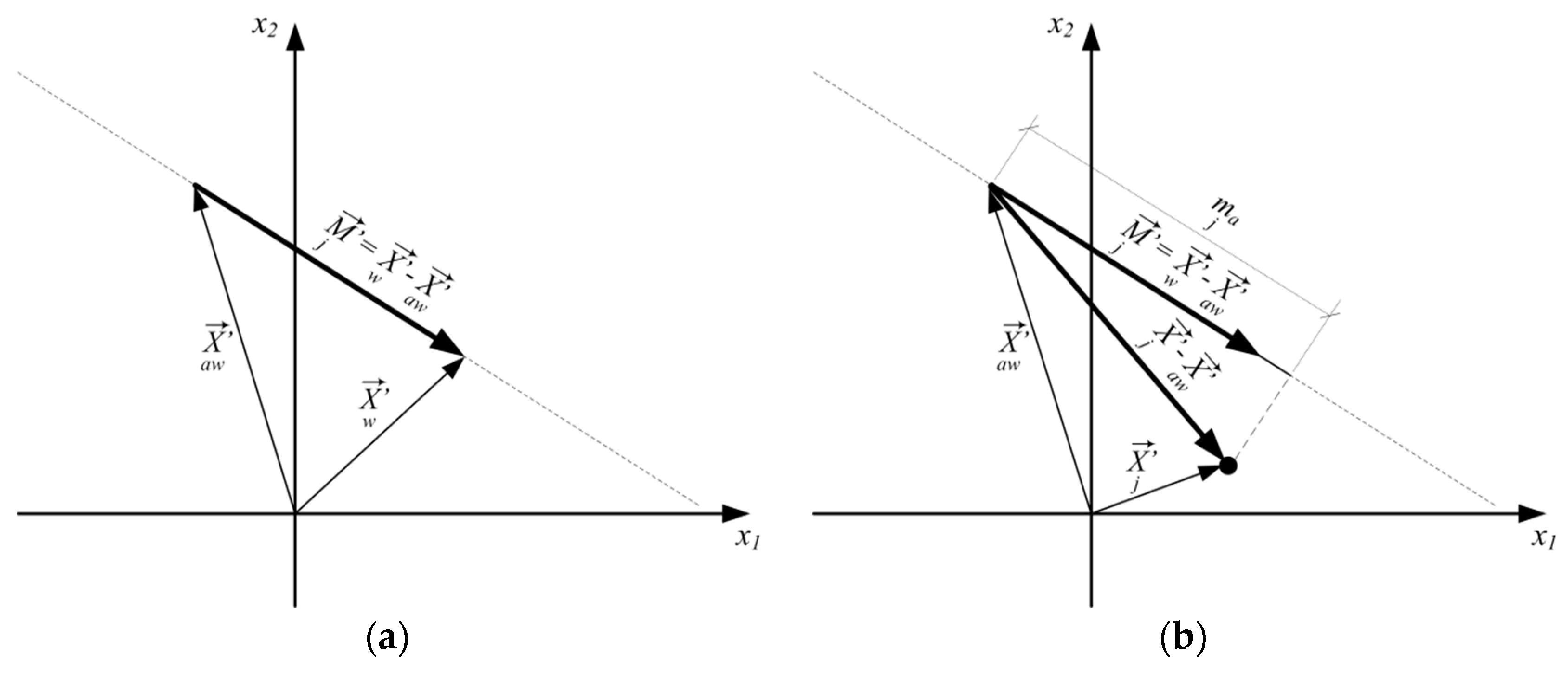
3.2.7. Stage 7. Construction of the Synthetic Measure

The values of the variables of the examined objects in the vector space are interpreted as vector coordinates. Each object therefore determines a specific direction in space. The pattern and anti-pattern difference is also a vector which determines a certain direction in space. Along this direction, the aggregate measure value for each object is calculated. This difference can be treated as a monodimensional coordinate system, in which the coordinates are calculated based on the formula [96,98]:
c = ( A , B ) ( B , B ) .
In turn, A and B are vectors, and ( A , B ) is the scalar product, which can be defined as follows:
( A , B ) = k = 1 n a k b k ,
where:
a k , b k —coordinates of the appropriate vector A and B .
We consider the B vector as the monodimensional coordinates system, thus it represents a difference between the pattern and anti-pattern. By entering coordinates of the pattern and anti-pattern as well as the object into the formula (18) the result is as follows [96,98]:
m a j     = i = 1 m ( x i j x i a w ) ( x i w x i a w ) i = 1 m ( x i w x i a w ) 2 .
For a synthetic measure so constructed, all objects that are better than the anti-pattern and worse than the pattern will have the measure value in the range from zero to one. The pattern will have the value equal to one and anti-pattern equal to zero. It is also possible to specify the value of the objects’ measure better than the pattern. They will have values greater than one. Objects that are worse than the anti-pattern will have a negative value of measure. Thanks to this, the position of the object in the ranking in relation to the pattern and anti-pattern will be easy to determinate.
In VMCM method a measuring vector M j is a difference between the vector of the pattern X w and the vector of the anti-pattern X a w (Figure 1a). The vector M j determines a monodimensional coordinates system having the origin in the point determined by the end of the vector of anti-pattern X a w . Aggregate measure m a j is the component (value of projection) of the vector X j X a w on the vector M j (Figure 1b).

3.2.8. Stage 8. Classification of Objects

The values of the aggregate measure allow for ranking objects; thus, it is possible to determine which of them are “better” and which are “worse”. They also allow the determination of which are similar to each other in terms of adopted criteria. To better visualize the results of calculations, objects can be divided into classes with similar measurement values. This is particularly important in the case of spatial objects. Such a ranking can be presented in the form of a map, where individual objects are visualized using the colors assigned to individual classes. In the simplest case objects can be classified based on mean value m ¯ m a 0 and standard deviation of the synthetic measure σ m a 0 . Objects are classified into four classes [94]:
{ 1   for   m a j     m ¯ m a 0 + σ m a 0 ;   )   ,   2   for   m a j     m ¯ m a 0 ; m ¯ m a 0 +   σ m a 0 )   , 3   for   m a j     m ¯ m a 0 σ m a 0 ;   m ¯ m a 0 )   ,   4   for   m a j     ( ; m ¯ m a 0 σ m a 0 ) .
It is also possible to classify objects into any number of classess by using quantiles:
{ 1   for   m a j     Q 0 n c ;   Q 1 n c ) , 2   for   m a j     Q 1 n c ;   Q 2 n c ) ,   n c   for   m a j     Q n c 1 n c   ;   Q n c n c ,
where:
Q k —quantile of the k-th order;
n c —number of classes.

3.3. The Course of the Research Experiment

The studies, both with the use of the TOPSIS and VMCM methods, were carried out based on the same data (SDGs-1 implementation indicators) and in the same period 2005–2016. The ranking of EU countries and their classification according to the poverty level (assignment to one of four groups according to the value of the aggregate measure) was made for two years, i.e., 2006 and 2016. To show differences in the usefulness of both methods for examining the dynamics of changes, two periods were considered for each of these years, based on which the matrix was created. Thus, for 2006 the matrix was created based on data from 2005–2009 and 2005–2016. However, for 2016 these were the following timeframes: 2005–2016 and 2010–2016. Such research assumptions made it possible, apart from obtaining a ranking of countries and their classification, to verify the applicability of the TOPSIS and VMCM methods for studying the dynamics of poverty level changes.

4. Results

First, poverty level analysis was carried out with the use of the TOPSIS method. The obtained results of the aggregate measure and the determined classification are presented in the tables below. To visualize better the results of the EU country classification, maps have been generated. Similar calculations were made with the other method (VMCM) and the results were presented in the same way as in case of the TOPSIS method. The final stage of the study was to examine the applicability of both methods for studying the dynamics of poverty, as shown in the charts.

4.1. TOPSIS Method

Calculations made with the use of the TOPSIS method, showing the classification of countries by poverty level in 2006 are presented in Table 2 and in Figure 2. Two timeframes for which matrices were created were analyzed (2005–2016 and 2005–2009).
Figure 2a shows the classification of the analyzed countries in relation to the matrix created based on data from 2005–2016 and Figure 2b in relation to the matrix created based on data from 2005–2009. Two differences can be observed in the classification (between Figure 2a,b). Due to a change in ranking (Table 2), which in this case had a direct impact on the classification (1 to 4), Ireland moved from Class 1 to Class 2, while Spain moved from Class 2 to Class 1. The results of the analyzes show that the poverty levels in these countries varied depending on the analytical period adopted for determining the matrix (2005–2016 or 2005–2009). This should not be the case, of course, and there should be no change in the ranking of countries, regardless of the period taken into account while creating the matrix. Moreover, it can be seen in Figure 2 (which should not be surprising) that the worst situation in terms of poverty level was recorded in countries newly acceded to the EU (Class 4), i.e., Hungary, Poland, Lithuania, Latvia, Romania, and Bulgaria. The worst result was achieved by Bulgaria. It is a group of so-called new EU member states, which joined the EU in 2004 and 2007.
Similar studies (conducted with the TOPSIS method) were carried out for the year 2016. Two timeframes (covering the year 2016) were analyzed, namely 2005-2016 and 2010-2016. Based on these periods, two matrices were created (reference points). The obtained ranking of the EU countries is presented in Table 3, while visualization of their classification is presented in Figure 3.
The classification of EU countries for 2016 based on the 2005–2016 matrix changed partly because of the creating the matrix taking into account the years 2010–2016. Slovakia, which was assigned to Class 2 (Figure 3a), moved to Class 3 (Figure 3b), Ireland moved from Class 3 to Class 2, Estonia moved from Class 3 to Class 4 and Italy moved from Class 4 to Class 3. As in the previous case study (2006), also in 2016, different ranking and classification results were obtained for some countries. Comparing the results obtained for 2016 (Table 3) and 2006 (Table 2), it can be seen that the situation in Poland and Hungary has improved. These countries have clearly benefited from the accession to the European Union, which is, moreover, in line with the EU’s support policy in this respect.

4.2. VMCM Method

Similar studies were carried out with the use of the VMCM method. They covered the same years (2006 and 2016) for rankings and different periods for creating the matrix (as with the TOPSIS method.) The obtained calculation results are presented in Table 4 and the visualization of the classification is presented in Figure 4.
Figure 4 shows the results of the 2006 and 2016 surveys classifying EU countries by level of poverty. The research conducted for 2006 for the adopted matrix from the periods 2005-2016 and 2005-2009 provided the same results (Figure 4a). The ranking of countries (Table 4), and consequently their classification (Class 1–4), is the same in both cases. A similar situation (the same results) is observed for the studies carried out for the year 2016 and two timeframes for the matrix creation (2005-2016 and 2010-2016), which is presented in Figure 4b.
The VMCM method (as well as the TOPSIS method) indicated that in 2006 the worst situation in terms of poverty (Class 4) occurred in Greece and in some of the new member states (Romania, Hungary, Bulgaria, Lithuania, Poland, and Latvia). In 2016, the situation of Poland and Hungary improved (from Class 4 to 3), while it deteriorated in Italy (from Class 3 to 4) and Greece dropped to the last place in the ranking.

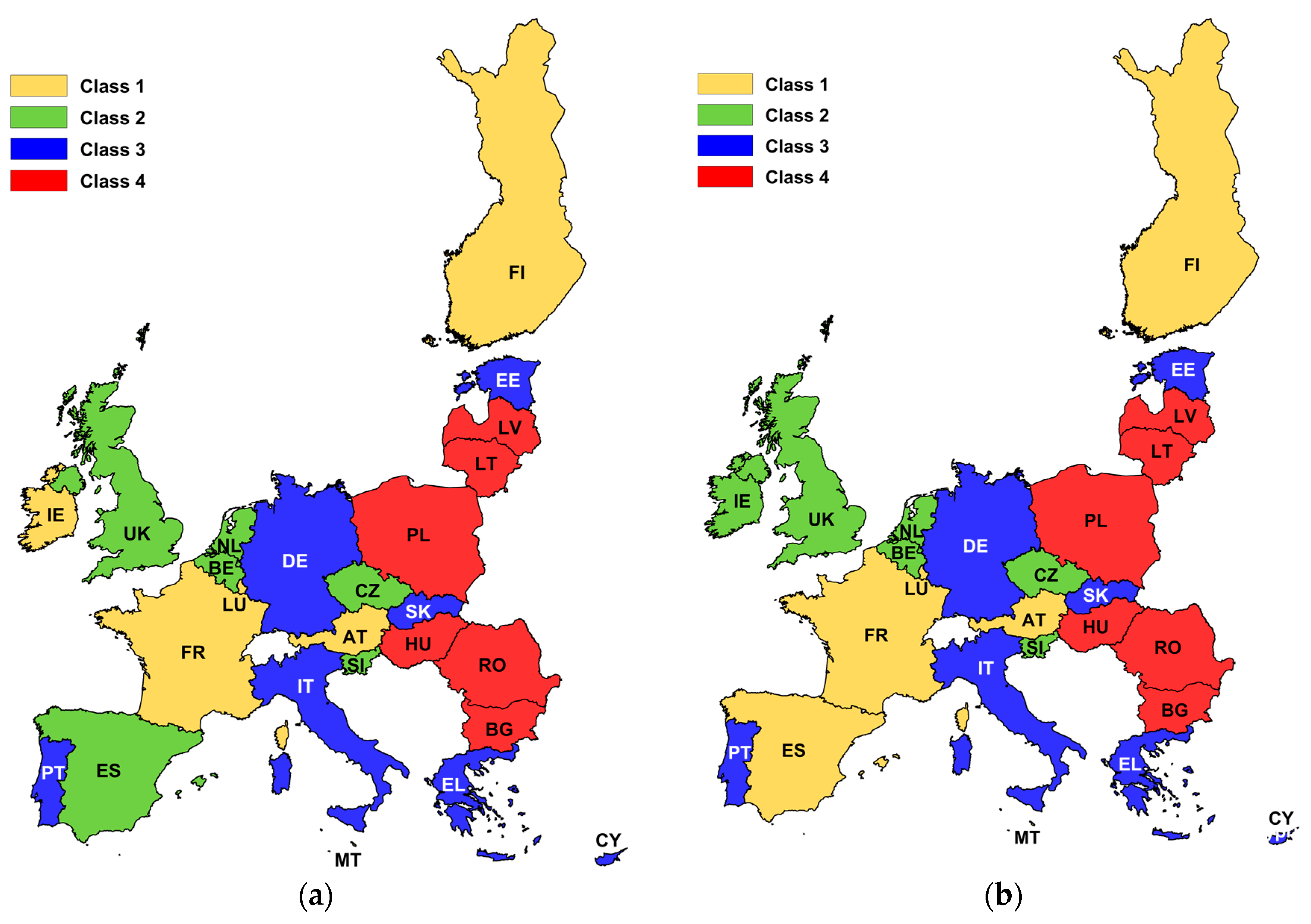
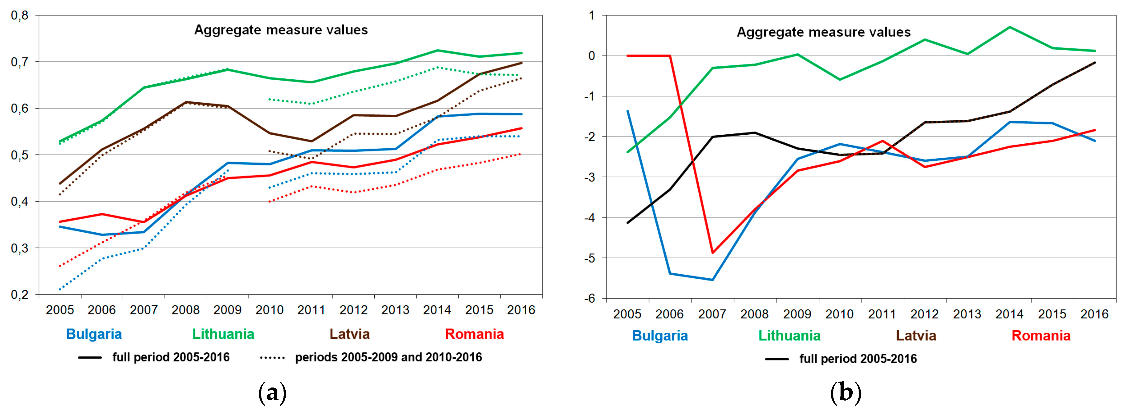
4.3. Analysis of the Dynamics of Changes: TOPSIS and VMCM

Following a study on the ranking and classification of the EU countries in the context of poverty, the applicability of the TOPSIS and VMCM methods for measuring the dynamics of changes was analyzed. The period 2005–2016 and its two sub-periods, namely 2005–2009 and 2010–2016, were analyzed (as in the previous surveys). 4 EU countries (Bulgaria, Latvia, Lithuania, and Romania) were selected for the survey, i.e., those with the highest differences in the aggregate measure value obtained for the two extreme years (2009 from the first sub-period in question and 2010 from the second sub-period). Figure 5a presents the results of the TOPSIS analysis of poverty dynamics, and Figure 5b presents the results of the VMCM analysis.
As can be seen in Figure 5a, segments of the charts for the years 2005–2009 and beyond 2010–2016 (dotted lines) do not coincide with the charts for the full period 2005–2016 (continuous lines). For example, for Romania (full period 2005–2016), the chart shows a slight increase in the aggregate poverty measure between 2009 and 2010. However, considering two time sections from the entire analysis period, i.e., the periods 2005–2009 and 2010–2016, a clear shift can be seen between the charts regarding these periods (a decrease in the aggregate measure value in 2010 in relation to 2009). Comparing the results for the period 2010–2016 with the results for the period 2005–2016, it should be noted that the chart of the aggregate measure value (2010–2016) is shifted downwards by approximately the same value. Moreover, charts for the years 2005–2009 and 2005–2016 are diverging in their initial phase (most for 2005). The above-mentioned takes place particularly in case of Bulgaria and Romania. In case of Lithuania, the difference is small and in case of Latvia, the two charts are practically the same (the fluctuations in the poverty level are minimal). The differences (shifts) visible in the chart between the full analyzed period (2005–2016) and its sections (2005–2009 and 2010–2016) are consequently of significant importance. Different aggregate measure values (for the same countries) mean that countries can change their position in the ranking and thus be assigned to different classes. Thus, for the first timeframes (2005–2009), changes in the aggregate measure value in relation to the period 2005–2016 had very little impact on the final ranking of the Warsaw Pact countries in terms of poverty levels. Out of 25 EU countries, 6 (representing 24% of the total sample) have changed their ranking position, with the changes in their ranking by one position. For the last analyzed year (2016), 9 countries (36%) changed their ranking by one position, and 3 countries (12%) changed their ranking by two positions.
Figure 5b illustrates the dynamics of poverty levels measured with the use of the VMCM method. The studies were carried out for the same timeframes (2005–2009, 2010-2016 and 2005–2016) as for the TOPSIS method. For the VMCM method, the charts for the period 2005–2009 and for the period 2010–2016 correspond exactly to the chart for the full period 2005–2016.
Comparing the results obtained with the use of the VMCM method with the results of the TOPSIS method, it can be seen that the VMCM method proved to be more sensitive to fluctuations and changes in the value of indicators. For Bulgaria, for example, the VMCM method showed a large decrease in the measure value between 2006 and 2007, while the TOPSIS method showed a small change in the measure value. When analyzing the source data, it can be seen that in these years (2006–2007) some indicators for Bulgaria demonstrated a sharp decrease. In the following year (2008) they were already higher than in 2007 and so the indicator sdg_01_40 increased by about 50%, the indicator sdg_01_50 increased by 40%, while the indicator sdg_01_30 increased by 30% and the indicator sdg_01_10 by 25%
Analyzing the values of the aggregate measure (Figure 5a,b) in the poverty level study (for the whole period 2005–2016), both methods (VMCM and TOPSIS) gave similar results in the ranking. In the context of the study on poverty dynamics, charts show significant differences between the two methods, showing that the VMCM method is more appropriate for studying the dynamics of changes.

5. Discussion

Research has shown that both the TOPSIS and the VMCM methods can be used to study poverty levels. Both methods enable the ranking and classification to be drawn up. However, the obtained results show that the VMCM method is more sensitive to changes in the data values taking into account in the calculations and it is more effective in case of new data which must be taken into account in the calculations (recreating of the matrix). In addition, the VMCM method allows the dynamics of changes to be studied and the TOPSIS method does not offer the possibility of obtaining reliable results in this case. Differences in the two methods are mainly due to the different methodological approaches used for the creation of the matrix. In the TOPSIS method the matrix should be the “best“ object for the whole analyzed period. Modifying this period in any way requires the matrix to be recreated from scratch. It also does not allow the use of actual or non-sample matrices. Figure 6a shows how the aggregate measure is determined by the TOPSIS method and explains its limitations.
In the TOPSIS method each object X j in the multidimensional space is between two objects v i + (ideal object, matrix) and object v i (negative ideal, negative matrix). Aggregate measure value Sj is the value given by the formula:
S j = d j d j + + d j ,
and it may be between 0 and 1. From the above formula and graphic illustration (Figure 6a) it follows that every new object requires a new identification of the ideal object v i + and negative ideal object v i . This is due to the risk that such an object may be located outside the limited area v i + and v i .
The VMCM method, on the other hand, eliminates the limitations of the TOPSIS method. The measure is not limited either from the bottom or from the top, which allows for better than the matrix objects, allows attachment of non-sample objects without the need of creating a new matrix and is more sensitive to the dynamics of changes (it allows examination of the dynamics). In the VMCM method the location of any object X j     in the multidimensional space (fig 6b) may be at any location in that space (and not as in the TOPSIS method within the area between limitations v i + and v i ). The aggregate measure m a j     constitutes in this method a vector component X j     X a w to a measuring vector M j = X w X a w . The measuring vector can be any object created based on sample data (with the use of I or III quartiles) or from outside the sample (any real object) and is not required that it needs to be an ideal object. Therefore, it is acceptable to consider objects better than the matrix. Then the aggregate measure value m a j     may be bigger than the unit. The aggregate measure values belong to one of the following groups (Figure 6b): m a j     > 0 (objects better than the matrix), m a j     0 ; 1 (the most common value, objects better than the negative matrix and worse than the matrix) or m a j     < 0 (objects worse than the negative matrix).
When comparing the TOPSIS and VMCM methods regarding the matrix determination, it can be seen (Figure 6) that in the TOPSIS method the object cannot be placed outside the area limited by an ideal and negative ideal object. Taking into account two different timeframes in the study, two different matrices must be created, where in each of them the ideal object and the negative ideal object can have different values. Therefore, in each such case the matrix should be recreated, and this makes it difficult to examine the dynamics of changes.
A proper study on economic phenomena, which, as with poverty, are usually multidimensional in nature, analyzing their dynamics of changes, or classifying analyzed objects (e.g., countries, regions) is of importance not only from the scientific point of view. The empirical and application qualities are also important. Sound empirical research, based on well-chosen methods of analysis, provides not only a good understanding of the nature and complexity of social and economic phenomena, but also of their results, which are typically used to guide policy-makers in their political and social activities [99]. This in turn should, from an economic point of view, lead to an increase in the effectiveness of spending funds on adequate public policies [100].

6. Conclusions

The article presents an original approach to the assessment of sustainable development in the context of analyzing the dynamics of changes in poverty levels (as one of the 17 objectives of the SDGs). The author’s VMCM dedicated to the study of complex economic phenomena described by many factors over time was applied. In contrast to commonly used approaches and techniques for assessing sustainable development (including poverty levels) based on ready-made indices or sets of indicators, a methodological solution is proposed that allows the creation of aggregate measurements with the use of any configuration of indicators. This approach is more universal and offers the possibility of creating aggregated measurements based on selected sets of indicators independently of the analyzed economic issues (e.g., in the areas of poverty, education, economic growth, etc., or sustainable development in general). The measures developed in this way can be freely modified (extended or narrowed down) and sets of diagnostic variables used can be altered. The proposed methodological approach (VMCM) is compared in the article with the TOPSIS (similar methodically) and verified based on actual SDGs (Eurostat) data from the same timeframes (2015–2016). In the context of creating rankings and classifications of EU countries in terms of poverty levels, both methods have proved their worth. However, the VMCM has proved to be more sensitive to changes in data values and more effective in situations where new variables are emerging that need to be included in the analyzes.
The issue of sustainable development analysis, including the level of poverty, requires constant monitoring in time and space. The commonly used indices allow for the analysis of a given phenomenon in a given year, but they do not allow for a direct analysis of its changes over time. Although it is possible to use the values of these indices (from given years) to examine tendencies of changes, they do not thoroughly explain changes in the analyzed phenomena over time, because there is no fixed point of reference in this case, and such a reference should be made to the same base year. The VMCM, using a unique methodical approach to the matrix creation, gives an opportunity to study the dynamics of changes over time. This is because the aggregate measure used in the calculations is not limited in multidimensional space, either from the bottom or from the top, so that objects which may be better than the accepted matrix may occur. The TOPSIS has a considerable limitation in this respect, namely, the location of the tested object must not be outside the area of the multidimensional space analyzed. This limitation means that the TOPSIS should not be used to analyze the dynamics of economic phenomena. As it is presented in the article, it did not prove useful in the analysis of poverty level changes, and thus, it will not prove useful in the examination of sustainable development progress (also regarding its other dimensions and aspects). On the other hand, the VMCM makes it possible to refer to an earlier established reference point (base year). It does not require the recreation of the matrix even if the object analyzed is better than the fixed matrix. This feature of the VMCM makes it ideal for studying economic phenomena which require analysis of their development over time. The presented analyzes of changes in poverty levels are an excellent example of the above-mentioned. Similarly, the VMCM can be used to explore other aspects of sustainable development.
In the light of the economic processes, the focus on the level of sustainable development in individual countries alone is insufficient. Indicators describing countries in terms of sustainable development are characterized by fluctuations over time, which is a result of changes taking place in these countries over the years and resulting from their functioning and development. The next step in the analysis may therefore be to examine time homogeneity, which allows us to see how these changes took place and to demonstrate the uniformity of their occurrence over time, which will make it possible to determine the degree of homogeneity of the country. Changes in the level of social and economic development of countries in time and space from the point of view of homogeneity may have a significant impact on their positions in rankings created according to various criteria. Therefore, the classification of countries according to their homogeneity is becoming an important issue, and its scope of use can be very helpful in the process of managing a given country or a group of countries, i.e., the EU. Measurement tools should therefore be used to take a broader view of the structure of countries. In this respect, among others, methods of studying time and spatial homogeneity may be applied. Therefore, another direction of research may be to adapt an appropriate methodological apparatus which would enable the analysis of time and spatial homogeneity of social and economic objects to the VMCM and the development of a fuzzy version of the VMCM for data expressed in a fuzzy form.

Author Contributions

Conceptualization, M.P., D.M., M.Ł., M.B. and K.N.; Data curation, M.P., M.B. and K.N.; Formal analysis, D.M. and M.Ł.; Methodology, M.P., M.B. and K.N.; Project administration, K.N.; Resources, D.M. and M.Ł.; Software, M.B.; Writing—original draft, M.P. and D.M.; Writing—review & editing, M.Ł.

Funding

This research received no external funding.

Conflicts of Interest

The authors declare no conflict of interest.

References

  1. Helne, T.; Hirvilammi, T. Wellbeing and Sustainability: A Relational Approach: Wellbeing and Sustainability. Sustain. Dev. 2015, 23, 167–175. [Google Scholar] [CrossRef]
  2. Schleicher, J.; Schaafsma, M.; Burgess, N.D.; Sandbrook, C.; Danks, F.; Cowie, C.; Vira, B. Poorer without It? The Neglected Role of the Natural Environment in Poverty and Wellbeing: The neglected role of the natural environment in poverty and wellbeing. Sustain. Dev. 2018, 26, 83–98. [Google Scholar] [CrossRef]
  3. Waas, T.; Hugé, J.; Block, T.; Wright, T.; Benitez-Capistros, F.; Verbruggen, A. Sustainability Assessment and Indicators: Tools in a Decision-Making Strategy for Sustainable Development. Sustainability 2014, 6, 5512–5534. [Google Scholar] [CrossRef] [Green Version]
  4. Arrow, K.J.; Dasgupta, P.; Goulder, L.H.; Mumford, K.J.; Oleson, K. Sustainability and the measurement of wealth: further reflections. Environ. Dev. Econ. 2013, 18, 504–516. [Google Scholar] [CrossRef]
  5. Bleys, B. The Regional Index of Sustainable Economic Welfare for Flanders, Belgium. Sustainability 2013, 5, 496–523. [Google Scholar] [CrossRef] [Green Version]
  6. Fleurbaey, M.; Blanchet, D. Beyond GDP: Measuring Welfare and Assessing Sustainability; Oxford University Press: Oxford, UK, 2013. [Google Scholar]
  7. Costanza, R.; Kubiszewski, I.; Giovannini, E.; Lovins, H.; McGlade, J.; Pickett, KE.; Ragnarsdóttir, K.V.; Roberts, D.; De Vogli, R.; Wilkinson, R. Development: Time to leave GDP behind. Nature 2014, 505, 283–285. [Google Scholar] [CrossRef] [PubMed] [Green Version]
  8. Fleurbaey, M. On sustainability and social welfare. J. Environ. Econ. Manag. 2015, 71, 34–53. [Google Scholar] [CrossRef]
  9. Dresner, S. The Principles of Sustainability, 2nd ed.; Routledge: Abingdon, UK, 2008. [Google Scholar]
  10. Ciegis, R.; Ramanauskiene, J.; Martinkus, B. The Concept of Sustainable Development and its Use for Sustainability Scenarios. Eng. Econ. 2009, 62, 2. [Google Scholar]
  11. Hedlund-de Witt, A. Rethinking Sustainable Development: Considering How Different Worldviews Envision “Development” and “Quality of Life”. Sustainability 2014, 6, 8310–8328. [Google Scholar] [CrossRef] [Green Version]
  12. Adler, M.D.; Fleurbaey, M.; Cowell, F. Inequality and Poverty Measures. In Oxford Handbook of Well-Being and Public Policy; Matthew, D.A., Marc, F., Eds.; Oxford University Press: Oxford, UK, 2016. [Google Scholar]
  13. Zheng, B. Aggregate Poverty Measures. J. Econ. Surv. 2002, 11, 123–162. [Google Scholar] [CrossRef] [Green Version]
  14. Haughton, J.H.; Khandker, S.R. Handbook on Poverty and Inequality; World Bank: Washington, DC, USA, 2009. [Google Scholar]
  15. Foster, J.; Seth, S.; Lokshin, M.; Sajaia, Z. A Unified Approach to Measuring Poverty and Inequality: Theory and Practice; The World Bank: Washington, DC, USA, 2013. [Google Scholar]
  16. Hellwig, Z. Application of the Taxonomic Method to the Countries Typology According to their Level of Development and the Structure of Resources and Qualified Staff. Przegląd Statystyczny 1968, 4, 307–326. (In Polish) [Google Scholar]
  17. Nermend, K. Metody Analizy Wielokryterialnej i Wielowymiarowej we Wspomaganiu Decyzji, 1st ed.; Wydawnictwo Naukowe PWN: Warszawa, Poland, 2017. [Google Scholar]
  18. Jajuga, K.; Marek, W.; Andrzej, B. On The General Distance Measure. In Exploratory Data Analysis in Empirical Research; Schwaiger, M., Opitz, O., Eds.; Springer: Berlin, Germany, 2003; pp. 104–109. [Google Scholar] [Green Version]
  19. Hwang, C.-L.; Yoon, K. Multiple Attribute Decision Making. In Lecture Notes in Economics and Mathematical Systems; Springer Nature Switzerland AG: Basel, Switzerland, 1981; Volume 186. [Google Scholar]
  20. Shen, K.Y.; Tzeng, G.H. Advances in Multiple Criteria Decision Making for Sustainability: Modeling and Applications. Sustainability 2018, 10, 1600. [Google Scholar] [CrossRef]
  21. Balcerzak, A.; Pietrzak, M. Application of TOPSIS Method for Analysis of Sustainable Development in European Union Countries. In Proceedings of the 10th International Days of Statistics and Economics, Prague, Czech Republic, 8–10 September 2016. [Google Scholar]
  22. Opricovic, S.; Tzeng, G.H. Compromise solution by MCDM methods: A comparative analysis of VIKOR and TOPSIS. Eur. J. Oper. Res. 2004, 156, 445–455. [Google Scholar] [CrossRef]
  23. Roy, B. ELECTRE III: Un algorithme de rangement fonde sur une representation floue des preferences en presence de criteres multiples. Cahiers du Centre d’etudes de recherche operationnelle. 1978, 20, 3–24. [Google Scholar]
  24. United Nations. Transforming our world: the 2030 Agenda for Sustainable Development. Available online: www.naturalcapital.vn/wp-content/uploads/2017/02/UNDP-Viet-Nam.pdf. (accessed on 15 April 2018).
  25. Waas, T.; Hugé, J.; Verbruggen, A.; Wright, T. Sustainable Development: A Bird’s Eye View. Sustainability 2011, 3, 1637–1661. [Google Scholar] [CrossRef] [Green Version]
  26. Strengers, Y.; Maller, C. (Eds.) Social Practices, Intervention and Sustainability: Beyond Behaviour Change (Routledge Studies in Sustainability); Routledge: Los Angeles, LA, USA, 2016. [Google Scholar]
  27. Hugé, J.; Waas, T.; Eggermont, G.; Verbruggen, A. Impact assessment for a sustainable energy future—Reflections and practical experiences. Energ. Pol. 2011, 39, 6243–6253. [Google Scholar] [CrossRef]
  28. Sachs, J.D. From Millennium Development Goals to Sustainable Development Goals. Lancet 2012, 379, 2206–2211. [Google Scholar] [CrossRef]
  29. UTCTAD. Development and Globalization: Facts and Figures. Available online: http://stats.unctad.org/Dgff2016/DGFF2016.pdf (accessed on 15 April 2018).
  30. Le Blanc, D. Towards Integration at Last? The Sustainable Development Goals as a Network of Targets: The sustainable development goals as a network of targets. Sustain. Dev. 2015, 23, 176–187. [Google Scholar] [CrossRef]
  31. World Commission on Environment and Development. Our Common Future. World Commission on Environment and Development; Oxford University Press: Oxford, UK, 1987. [Google Scholar]
  32. Beisheim, M.; Løkken, H.; Aus, D.M.N.; Pintér, L.; Rickels, W. Measuring Sustainable Development: How Can Science Contribute to Realizing the SDGs? SWP Berlin: Berlin, Germany, 2015; Volume 8, pp. 1–32. [Google Scholar]
  33. MacFeely, S. Measuring the Sustainable Development Goals: What does it mean for Ireland? Administration 2017, 65, 41–71. [Google Scholar] [CrossRef]
  34. Rieckmann, M. Education for Sustainable Development Goals: Learning Objectives; UNESCO: Paris, France, 2017. [Google Scholar]
  35. International Council for Science. A Guide to SDG Interactions: From Science to Implementation; International Council for Science: Paris, France, 2017. [Google Scholar]
  36. Eurostat. Sustainable Development in the European Union: Monitoring Report on Progress towards the SDGs in an EU Context; Publications office of the European Union: Luxemburg, 2017. [Google Scholar]
  37. European Commission. Communication from the Commission to the European Parliament, the Council, the European Economic and Social Committee and the Committee of the Regions Next Steps for A Sustainable European Future—European Action for Sustainability. Available online: https://ec.europa.eu/europeaid/sites/devco/files/communication-next-steps-sustainable-europe-20161122_en.pdf (accessed on 15 April 2018).
  38. Barkin, D.; Lemus, B. Understanding Progress: A Heterodox Approach. Sustainability 2013, 5, 417–431. [Google Scholar] [CrossRef] [Green Version]
  39. Spicker, P.; Álvarez Leguizamón, S.; Gordon, D. Comparative Research Programme on Poverty; Zed Books: London, UK, 2007. [Google Scholar]
  40. Hagenaars, A.; de Vos, K. The Definition and Measurement of Poverty. J. Hum. Resource. Manag. 1988, 23, 211–221. [Google Scholar] [CrossRef]
  41. Foster, J.E. Absolute versus Relative Poverty. Am. Econ. Rev. 1998, 88, 335–341. [Google Scholar]
  42. Lok-Dessallien, R. Review of Poverty Concepts and Indicators. Available online: https://pdfs.semanticscholar.org/a358/eb2139bf8c50b338863d0ecb63d4c6dedb21.pdf (accessed on 15 June 2018).
  43. Weziak-Bialowolska, D.; Dijkstra, L. Regional Human Poverty Index: Poverty in the Regions of the European; Publications office of the European Union: Luxemburg, 2014. [Google Scholar]
  44. Sen, A. Inequality Reexamined; Oxford University Press: New York, NY, USA, 2004. [Google Scholar]
  45. Alkire, S.; Santos, M.E. A Multidimensional Approach: Poverty Measurement & Beyond. Soc. Indicat. Res. 2013, 112, 239–257. [Google Scholar] [Green Version]
  46. Alkire, S.; Foster, J. Counting and multidimensional poverty measurement. J. Publ. Econ. 2011, 95, 476–487. [Google Scholar] [CrossRef]
  47. Alkire, S.; Foster, J. Understandings and misunderstandings of multidimensional poverty measurement. J. Econ. Inequal. 2011, 9, 289–314. [Google Scholar] [CrossRef] [Green Version]
  48. Antony, G.M.; Visweswara Rao, K. A composite index to explain variations in poverty, health, nutritional status and standard of living: Use of multivariate statistical methods. Publ. Health. 2007, 121, 578–587. [Google Scholar] [CrossRef] [PubMed]
  49. Bellani, L. Multidimensional indices of deprivation: The introduction of reference groups weights. J. Econ. Inequal. 2013, 11, 495–515. [Google Scholar] [CrossRef]
  50. Betti, G.; Gagliardi, F.; Lemmi, A.; Verma, V. Subnational indicators of poverty and deprivation in Europe: Methodology and applications. Camb. J. Regions. Econ. Soc. 2012, 5, 129–147. [Google Scholar] [CrossRef]
  51. Ravallion, M. On multidimensional indices of poverty. J. Econ. Inequal. 2011, 9, 235–248. [Google Scholar] [CrossRef]
  52. Wagle, U. Multidimensional Poverty Measurement; Springer US: New York, NY, USA, 2008; ISBN 978-0-387-75874-9. [Google Scholar]
  53. Sen, A. Poor, Relatively Speaking. Oxf. Econ. Paper. 1983, 35, 153–169. [Google Scholar] [CrossRef]
  54. Sen, A. Commodities and Capabilities; Oxford University Press: Oxford, UK, 1986. [Google Scholar]
  55. Tsui, K. Multidimensional poverty indices. Soc. Choice. Welfare. 2002, 19, 69–93. [Google Scholar] [CrossRef] [Green Version]
  56. Atkinson, A.B. Multidimensional Deprivation: Contrasting Social Welfare and Counting Approaches. J. Econ. Inequal. 2003, 1, 51–65. [Google Scholar] [CrossRef]
  57. Bourguignon, F.; Chakravarty, S.R. Multidimensional Poverty Orderings: Theory and Applications. In Arguments for a Better World: Essays in Honor of Amartya Sen; Oxford University Press: Oxford, UK, 2008. [Google Scholar]
  58. Duclos, J.-Y.; Luca Tiberti, L. Multidimensional Poverty Indices: A Critical Assessment. In the Oxford Handbook of Well-Being and Public Policy; Adler, M.D., Fleurbaey, M., Eds.; Oxford University Press: New York, NY, USA, 2016. [Google Scholar]
  59. Alkire, S. The Capability Approach and Well-Being Measurement for Public Policy. Available online: https://www.ophi.org.uk/wp-content/uploads/OPHIWP094.pdf. (accessed on 15 June 2018).
  60. Chakravarty, S.R.; Mukherjee, D.; Ranade, R.R. On the family of subgroup and factor decomposable measures of multidimensional poverty. Res. Econ. Inequal. Res. Annu. 1998, 8, 175–194. [Google Scholar]
  61. Bourguignon, F.; Chakravarty, S. The Measurement of Multidimensional Poverty. J. Econ. Inequal. 2003, 1, 25–49. [Google Scholar] [CrossRef]
  62. Chakravarty, S.R.; D’Ambrosio, C. The Measurement of Social Exclusion. Rev. Income Wealth 2006, 52, 377–398. [Google Scholar] [CrossRef]
  63. Chakravarty, S.R.; Silber, J. Measuring Multidimensional Poverty: The Axiomatic Approach. In Quantitative Approaches to Multidimensional Poverty Measurement; Kakwani, N., Silber, J., Eds.; Palgrave Macmillan: London, UK, 2008; pp. 192–209. [Google Scholar]
  64. Bossert, W.; Chakravarty, S.R.; D’Ambrosio, C. Multidimensional Poverty and Material Deprivation with Discrete Data. Rev. Income Wealth 2013, 59, 29–43. [Google Scholar] [CrossRef]
  65. Maasoumi, E.; Lugo Maria, A. The Information Basis of Multivariate Poverty Assessments. In Quantitative Approaches to Multidimensional Poverty Measurement; Kakwani, N., Silber, J., Eds.; Palgrave Macmillan: London, UK, 2008; pp. 1–29. [Google Scholar]
  66. Silber, J. Economic Studies in Inequality, Social Exclusion and Well-Being. In Fuzzy Set Approach to Multidimensional Poverty Measurement; Lemmi, A., Betti, G., Eds.; Springer: New York, NY, USA, 2006; Volume 3. [Google Scholar]
  67. Kakwani, N.C.; Silber, J. Quantitative Approaches to Multidimensional Poverty Measurement; Palgrave Macmillan: Basingstoke, UK, 2008. [Google Scholar]
  68. Asselin, L.-M. Analysis of Multidimensional Poverty: Theory and Case Studies; Springer New York: New York, NY, USA, 2009. [Google Scholar]
  69. UN Development Programme (UNDP). The Rise of the South: Human Progress in a Diverse World; United Nations Development Programme: New York, NY, USA, 2013. [Google Scholar]
  70. Kevin, W. Human Development Report 2007/2008. Available online: http://hdr.undp.org/sites/default/files/hdr_20072008_summary_english.pdf (accessed on 17 June 2018).
  71. Sabina, A.; Maria, E.S. Measuring Acute Poverty in the Developing World: Robustness and Scope of the Multidimensional Poverty Index. World Dev. 2013, 59, 251–274. [Google Scholar]
  72. Alkire, S.; Santos, M.E.; Seth, S.; Gaston, Y. Is the Multidimensional Poverty Index Robust to Different Weights? Available online: https://ophi.org.uk/ophi-research-in-progress-22a/ (accessed on 17 June 2018).
  73. Cornford, A. Multidimensional Poverty and its Measurement. In Guide on Poverty Measurement; United Nations Economic Commission for Europe: Geneva, The Switzerland, 2016. [Google Scholar]
  74. Walesiak, M. Multivariate Statistical Analysis in Marketing Research. Available online: http://keii.ue.wroc.pl/pracownicy/mw/1993_Walesiak_SAW_w_badaniach_marketingowych_OCR.pdf (accessed on 20 February 2018). (In Polish).
  75. Tarczyński, W. A Taxonomic Measure of the Attraction of Investments in Securities. Przegląd Statystyczny 1994, 41, 275–300. (In Polish) [Google Scholar]
  76. Opricovic, S. Multicriteria Optimization of Civil Engineering Systems. Fac. Civ. Eng. Belgrad. 1998, 2, 5–21. [Google Scholar]
  77. Mardani, A.; Zavadskas, E.K.; Khalifah, Z.; Zakuan, N.; Jusoh, A.; Nor, K.M.; Khoshnoudi, M. A review of multi-criteria decision-making applications to solve energy management problems: Two decades from 1995 to 2015. Renew. Sustain. Energ. Rev. 2017, 71, 216–256. [Google Scholar] [CrossRef]
  78. Wątróbski, J.; Małecki, K.; Kijewska, K.; Iwan, S.; Karczmarczyk, A.; Thompson, R. Multi-Criteria Analysis of Electric Vans for City Logistics. Sustainability 2017, 9, 1453. [Google Scholar] [CrossRef]
  79. Mardani, A.; Zavadskas, E.K.; Govindan, K.; Amat Senin, A.; Jusoh, A. VIKOR Technique: A Systematic Review of the State of the Art Literature on Methodologies and Applications. Sustainability 2016, 8, 37. [Google Scholar] [CrossRef] [Green Version]
  80. Jankowski, J.; Zioło, M.; Karczmarczyk, A.; Wątróbski, J. Towards Sustainability in Viral Marketing with User Engaging Supporting Campaigns. Sustainability 2017, 10, 15. [Google Scholar] [CrossRef]
  81. Wu, D.; Yang, Z.; Wang, N.; Li, C.; Yang, Y. An Integrated Multi-Criteria Decision Making Model and AHP Weighting Uncertainty Analysis for Sustainability Assessment of Coal-Fired Power Units. Sustainability 2018, 10, 1700. [Google Scholar] [CrossRef]
  82. Erdogan, S.; Sayin, C. Selection of the Most Suitable Alternative Fuel Depending on the Fuel Characteristics and Price by the Hybrid MCDM Method. Sustainability 2018, 10, 1583. [Google Scholar] [CrossRef]
  83. Wątróbski, J.; Ziemba, P.; Jankowski, J.; Zioło, M. Green Energy for a Green City—A Multi-Perspective Model Approach. Sustainability 2016, 8, 702. [Google Scholar] [CrossRef]
  84. Kumar, A.; Sah, B.; Singh, A.R.; Deng, Y.; He, X.; Kumar, P.; Bansal, R.C. A review of multi criteria decision making (MCDM) towards sustainable renewable energy development. Renew. Sustain. Energ. Rev. 2017, 69, 596–609. [Google Scholar] [CrossRef]
  85. Jahanshahloo, G.R.; Lotfi, F.H.; Izadikhah, M. An algorithmic method to extend TOPSIS for decision-making problems with interval data. Appl. Math. Comput. 2006, 175, 1375–1384. [Google Scholar] [CrossRef]
  86. Jahanshahloo, G.R.; Lotfi, F.H.; Davoodi, A.R. Extension of TOPSIS for decision-making problems with interval data: Interval efficiency. Math. Comput. Model. 2009, 49, 1137–1142. [Google Scholar] [CrossRef]
  87. Zavadskas, E.K.; Mardani, A.; Turskis, Z.; Jusoh, A.; Nor, K.M. Development of TOPSIS method to solve complicated decision-making problems: An overview on developments from 2000 to 2015. Int. J. Inform. Tech. Decis. 2016, 15, 645–682. [Google Scholar] [CrossRef]
  88. Liu, C.; Zhang, R.; Wang, M.; Xu, J. Measurement and Prediction of Regional Tourism Sustainability: An Analysis of the Yangtze River Economic Zone, China. Sustainability 2018, 10, 1321. [Google Scholar] [CrossRef]
  89. Niu, D.; Li, Y.; Dai, S.; Kang, H.; Xue, Z.; Jin, X.; Song, Y. Sustainability Evaluation of Power Grid Construction Projects Using Improved TOPSIS and Least Square Support Vector Machine with Modified Fly Optimization Algorithm. Sustainability 2018, 10, 231. [Google Scholar] [CrossRef]
  90. Yang, W.; Liu, L.; Yu, X. Evaluating the Comprehensive Benefit of Group-Affiliated New Energy Power Generation Enterprises for Sustainability: Based on a Combined Technique of STBI and TOPSIS. Sustainability 2017, 10, 24. [Google Scholar] [CrossRef]
  91. You, P.; Guo, S.; Zhao, H.; Zhao, H. Operation Performance Evaluation of Power Grid Enterprise Using a Hybrid BWM-TOPSIS Method. Sustainability 2017, 9, 2329. [Google Scholar] [CrossRef]
  92. Lu, C.; Xue, B.; Lu, C.; Wang, T.; Jiang, L.; Zhang, Z.; Ren, W. Sustainability Investigation of Resource-Based Cities in Northeastern China. Sustainability 2016, 8, 1058. [Google Scholar] [CrossRef]
  93. Zhao, H.; Li, N. Performance Evaluation for Sustainability of Strong Smart Grid by Using Stochastic AHP and Fuzzy TOPSIS Methods. Sustainability 2016, 8, 129. [Google Scholar] [CrossRef]
  94. Nermend, K. Vector Calculus in Regional Development Analysis: Comparative Regional Analysis Using the Example of Poland (Contributions to economics); Physica-Verlag: Verlag, Germany, 2009. [Google Scholar]
  95. Kukuła, K. Metoda Unitaryzacji Zerowanej; Wydaw. Naukowe PWN: Warszawa, Poland, 2000; ISBN 978-83-01-13097-8. (In Polish) [Google Scholar]
  96. Nermend, K. Taxonomic Vector Measure of Region Development (TWMRR). Pol. J. Environ. Stud. 2007, 16, 195–198. [Google Scholar]
  97. Dodge, Y. The Concise Encyclopedia of Statistics, 1st ed.; Springer: New York, NY, USA, 2008. [Google Scholar]
  98. Nermend, K. A synthetic measure of sea environment pollution. Pol. J. Environ. Stud. 2006, 15, 127–129. [Google Scholar]
  99. Boţa-Avram, C.; Groşanu, A.; Răchişan, P.-R.; Gavriletea, M. The Bidirectional Causality between Country-Level Governance, Economic Growth and Sustainable Development: A Cross-Country Data Analysis. Sustainability 2018, 10, 502. [Google Scholar] [CrossRef]
  100. Gruber, J. Public Finance and Public Policy, 5th ed.; Worth Publishers: New York, NY, USA, 2005. [Google Scholar]
Figure 1. Measure value depending on the object’s position (a) measuring vector M j ; (b) aggregate measure m a j .
Sustainability 10 02858 g001
Figure 2. Results of the classification (TOPSIS) of the EU countries in 2006 regarding the poverty level for the reference period covering years: (a) 2005—2016; (b) 2005—2009.
Sustainability 10 02858 g002
Figure 3. Results of the classification (TOPSIS) of the EU countries in 2016 regarding the poverty level for the reference period covering years: (a) 2005–2016; (b) 2010–2016.
Sustainability 10 02858 g003
Figure 4. Results of the classification (VMCM) of the EU countries by poverty level for year: (a) 2006 (matrix for the years 2005-2016 and 2005–2009); (b) 2016 (2005–2016 and 2010–2016).
Sustainability 10 02858 g004
Figure 5. Comparison of results regarding analyzes of the dynamics of poverty changes (aggregate measure values) in years 2005–2016 and 2005–2009, 2010–2016, with the use of methods: (a) TOPSIS; (b) VMCM.
Sustainability 10 02858 g005
Figure 6. Determination of the aggregate measure value for the analyzed object in multidimensional space in relation to the matrix and the negative matrix: (a) TOPSIS; (b) VMCM.
Sustainability 10 02858 g006
Table 1. Comparison of Millennium Development Goals and Sustainable Development Goals–basic information [24,28].
MDGsSDGs
They were meant to be an effective method of global mobilization to achieve a set of important social priorities worldwide, but they were mainly addressed to developing countries.They are intended to be a universal development plan, adapted to different contexts, suitable for all nations (poor and rich, developed and developing) and organizations (of public, private and third sector) that work together.
8 isolated objectives with 21 tasks, limited focus on sustainable development.17 objectives and 169 related tasks, interdependent and indivisible, ensuring a balance between three aspects of sustainable development: economic, social, and environmental.
Goals:
  • Eradicate extreme poverty and hunger
  • Achieve universal primary education
  • Promote gender equality and empower women
  • Reduce child mortality
  • Improve maternal health
  • Combat HIV/AIDS, malaria, and other diseases
  • Ensure environmental sustainability
  • Develop a global partnership for development
Goals:
  • No poverty
  • Zero hunger
  • Good health and well-being
  • Quality education
  • Gender equality
  • Clean water and sanitation
  • Affordable and clean Energy
  • Decent work and economic growth
  • Industry, innovation, and infrastructure
  • Reduced inequalities
  • Sustainable cities and communities
  • Responsible consumption and production
  • Climate action
  • Life below water
  • Life on land
  • Peace, justice, and strong institutions
  • Partnership for the goals
Coordinated by the UN Secretariat.Negotiated by UN member states over a three-year period, in the framework of a broad multi-stakeholder consultation.
Implementation measures are limited to North-South financial flows; poor reporting, follow-up, and review (assessment).Implementation measures include market access, technology transfer, production capacity, development, and policy support; a robust global architecture for monitoring, and review (assessment).
Table 2. Ranking of EU countries in 2006 (TOPSIS) for two reference timeframes.
CountryAggregate Measure ValueClassCountryAggregate Measure ValueClass
Matrix 2005—2016Matrix 2005—2009
Luxembourg (LU)0.9191881Luxembourg (LU)0.91953121
Finland (FI)0.90877911Finland (FI)0.9098131
Austria (AT)0.90601521Austria (AT)0.90464561
Malta (MT)0.89412681Malta (MT)0.89102491
France (FR)0.89192191France (FR)0.89009521
Ireland (IE)0.86309271Spain0.85637461
Spain (ES)0.86046332Ireland (IE)0.8520282
Slovenia (SI)0.83433862Slovenia (SI)0.83482772
Belgium (BE)0.83058242Belgium (BE)0.81902732
Netherlands (NL)0.81952082Czech Republic0.80943222
United Kingdom (UK)0.81606912Netherlands (NL)0.80896582
Czech Republic (CZ)0.81096512United Kingdom (UK)0.80555872
Germany (DE)0.80119313Germany (DE)0.79408883
Italy (IT)0.7810043Italy (IT)0.77643963
Slovakia (SK)0.75326663Slovakia (SK)0.75350743
Cyprus (CY)0.75090633Cyprus (CY)0.75016833
Portugal (PT)0.73592363Portugal (PT)0.73672523
Estonia (EE)0.72090043Estonia (EE)0.72472063
Greece (EL)0.70969233Greece0.70481033
Hungary (HU)0.698364Hungary (HU)0.69386934
Poland (PL)0.58276574Poland (PL)0.57375774
Lithuania (LT)0.57353864Lithuania (LT)0.57096374
Latvia (LV)0.51198764Latvia (LV)0.49876534
Romania (RO)0.37308334Romania (RO)0.31180624
Bulgaria (BG)0.32860864Bulgaria (BG)0.27724994
Table 3. Ranking of EU countries in 2016 (TOPSIS) for two reference timeframes.
CountryAggregate Measure ValueClassCountryAggregate Measure ValueClass
Matrix 2005–2016Matrix 2010–2016
Malta (MT)0.91389411Malta (MT)0.91479671
Austria (AT)0.89731681Austria (AT)0.89368521
France (FR)0.88903681France (FR)0.89222091
Czech Republic (CZ)0.88887291Finland (FI)0.88672951
Finland (FI)0.87950071Czech Republic (CZ)0.88385271
Netherlands (NL)0.87545921Netherlands (NL)0.87421721
Luxembourg (LU)0.87422122Luxembourg (LU)0.86859152
Slovenia (SI)0.86769482Slovenia (SI)0.85677462
Germany (DE)0.84438962United Kingdom (UK)0.8389132
United Kingdom (UK)0.84218192Germany (DE)0.83804222
Slovakia (SK)0.83653262Belgium (BE)0.83057742
Belgium (BE)0.83068652Ireland (IE)0.82188812
Ireland (IE)0.81992873Spain (ES)0.81214883
Spain (ES)0.81606133Slovakia (SK)0.80636533
Portugal (PT)0.7814453Cyprus (CY)0.76175563
Cyprus (CY)0.77465193Poland (PL)0.755653
Poland (PL)0.7733163Portugal (PT)0.75284913
Estonia (EE)0.76835463Hungary (HU)0.73784583
Hungary (HU)0.76369773Italy (IT)0.71686313
Italy (IT)0.73793074Estonia (EE)0.71674424
Lithuania (LT)0.71871714Lithuania (LT)0.67133094
Latvia (LV)0.69743774Latvia (LV)0.66486964
Bulgaria (BG)0.58724424Bulgaria (BG)0.53959874
Romania (RO)0.55738894Greece (EL)0.5225154
Greece (EL)0.555324Romania (RO)0.50192614
Table 4. Ranking of EU countries in 2006 and 2016 (VMCM) for two reference timeframes.
CountryAggregate Measure ValueClassCountryAggregate Measure ValueClass
Year 2006, Matrix 2005—2016 and 2005—2009Year 2016, Matrix 2005—2016 and 2010—2016
Finland (FI)4.3484071Finland (FI)4.1749761
Luxembourg (LU)4.0048481Czech Republic (CZ)3.8015521
Austria (AT)3.8530231Malta (MT)3.6910671
Malta (MT)4.0238141Austria (AT)3.4856771
France (FR)3.5708471France (FR)3.3538171
Slovenia (SI)3.0045492Netherlands (NL)3.0154862
Netherlands (NL)2.8197452Slovenia (SI)2.6866042
Ireland (IE)2.7008682Slovakia (SK)2.5566052
Belgium (BE)2.4867022Luxembourg (LU)2.5383982
Spain (ES)2.2898932Ireland (IE)2.2383622
Czech Republic (CZ)2.3805582United Kingdom (UK)2.2307182
Germany (DE)2.1157423Belgium (BE)2.2248042
United Kingdom (UK)1.5355273Estonia (EE)2.1134013
Cyprus (CY)2.0395383Germany (DE)2.0441793
Portugal (PT)1.5173063Poland (PL)1.7985743
Slovakia (SK)1.6790373Cyprus (CY)1.7274533
Italy (IT)0.59703573Spain (ES)1.2068373
Estonia (EE)0.63938453Hungary (HU)1.035743
Romania (RO)04Portugal (PT)0.90273413
Greece (EL)−0.76347194Italy (IT)0.16223124
Hungary (HU)−0.51042984Lithuania (LT)0.11790274
Bulgaria (BG)−5.3866814Latvia (LV)−0.17515124
Lithuania (LT)−1.530164Romania (RO)−1.8405484
Poland (PL)−2.8075854Bulgaria (BG)−2.1006714
Latvia (LV)−3.3045774Greece (EL)−3.1463094

