Article

Short and Long-Term Temporal Changes in Air Quality in a Seoul Urban Area: The Weekday/Sunday Effect

1
Department of Civil and Environmental Engineering, Hanyang University, 222 Wangsimni-Ro, Seoul 04763, Korea
2
Department of Marine Science and Technology, The Federal University of Technology, P.M.B. 704, Akure, Nigeria
3
Environmental and Water Resources Engineering Division, Department of Civil Engineering, IIT Madras, Chennai 600 036, India
4
Department of Environment & Energy, Sejong University, Seoul 05006, Korea
5
College of Pharmacy, Kyung Hee University, Seoul 02447, Korea
6
Chemical, Medical and Environmental Science Department, National Physical Laboratory, Teddington, Middlesex TW11 0LW, UK
*
Author to whom correspondence should be addressed.
Sustainability 2018, 10(4), 1248; https://doi.org/10.3390/su10041248
Submission received: 15 March 2018 / Revised: 15 April 2018 / Accepted: 17 April 2018 / Published: 19 April 2018

Abstract

:
We present evidence on the short-term differences in airborne pollution levels in terms of weekday/weekend (WD/WN) and weekday/Sunday (WD/Sun) intervals. To this end, we analyzed the hourly data of important pollutants (nitric oxide (NO), nitrogen dioxide (NO2), ozone (O3) and carbon monoxide (CO)) using the data acquired in the Yong-San district of Seoul, Korea from 2009 to 2013. For each week, the pollutant ratio (Rw) was estimated through either WD/WN or WD/Sun. Here, a week is defined as Sunday through Saturday, WD as Monday through Friday and WN as Sunday and Saturday. The WD/Sun Rw geometric means (and range) were 2.02 (0.27–15.5) for NO, 1.29 (0.49–5.7) for NO2 and 0.89 (0.17–7.2) for O3 while the fraction of Rw (WD/Sun) > 1 were 81, 71 and 38%, respectively. NO and CO levels were much higher in October through March (during Autumn and Winter) than April through September (during Spring and Summer), reflecting the potential effect of fuel consumption (e.g., in terms of use patterns of nationwide city natural gas). Thus, we provide a broader interpretation on the occurrence patterns of the major pollutants (e.g., NO, NO2, O3 and CO) in relation to temporal changes in man-made activities.

1. Introduction

The combustion of fossil fuels, especially for power generation, domestic heating and transportation purposes and so forth, is the main source of air pollution. Of these, transportation-related air pollutants (TRAPs) are most difficult to control because of the increasing vehicle usage in growing economies, especially in developing countries.
A number of natural processes (such as lightning, volcanic eruptions, bacterial activity in soil, forest fires, production of biogenic compounds and photochemical degradation of nitrogen compounds in the upper atmosphere) release considerable amounts of NOx into the troposphere. Nonetheless, TRAP-derived NOx (a mixture of NO and NO2) account for most of the elevated NOx levels observed in major cities [1]. The levels of roadside NOx increase with traffic density, especially during ‘rush hours’; hence, NOx is a reliable marker of road-traffic emissions [2]. The higher pressures and temperatures found in internal combustion engines (especially diesels compared to natural gas furnaces for heating) favor the formation of NO from N2 and O2 precursors in the endothermic reaction (NIST Chemistry Webbook) [3,4,5,6].
Besides being noxious to humans, NOx also leads to secondary atmospheric pollution, for example, the formation of aerosols and acid rain [7]. From an agricultural perspective, such secondary pollution could reduce soil and water quality, thereby hindering plant growth [8]. About 90% of the tropospheric NOx is estimated to be from primary NO emissions whereas NO2 is an oxidation product of NO by O3 [9]. For the interested reader, atmospheric chemistry and physics has been comprehensively reviewed [10].
Ozone in the stratosphere is generally found at higher concentrations (e.g., at low ppm levels) than those at ground level (e.g., at ppb levels) and is important for absorbing solar UV radiation (http://www.ozonelayer.noaa.gov/science/basics.htm). However, tropospheric O3 is a pollutant, a product of both natural and anthropogenic processes, mainly formed through the photochemical oxidation of NO, methane (CH4), non-methane hydrocarbons (NMHCs) and carbon monoxide (CO) [11,12,13]. More specifically, the combined effects of volatile organic compounds (VOCs) and NOx control on the formation of O3 near the Earth’s surface. Given the complex non-linear route of O3 formation, its formation-removal varies day-by-day and from site-to-site depending on many factors (e.g., sunlight and VOC levels). Changes in the spatial and temporal distribution of O3 can also be affected sensitively by meteorological factors such as ultraviolet (UV) radiation intensity, temperature (T), solar radiance (SR), wind speed (V) and relative humidity (RH). The combined effect of these natural factors can facilitate the production, loss, conversion and dispersion of atmospheric oxidants (such as O3).
The influence of human activities on local (e.g., urban) and regional (urban plus rural) air pollution has previously been investigated on a weekly basis [14,15,16,17,18,19,20,21]. Masiol et al. [22] reported 13-year trends in NOx and O3 levels, along with those of CO, SO2 and PM10 (particulate matter of sizes < 10 µm). It has been suggested that the differences in pollution between weekday (WD: Monday through Friday) and weekend (WN: Saturday and Sunday) periods can influence the local climate in the coastal NW Atlantic region of the USA as rainfall is higher on weekends [23]. On the other hand, rainfall was reported to be higher during midweek in south east USA due in part to higher anthropogenic air pollution [24]. In an area east of the Mississippi River in the USA, the higher summer precipitation on Tuesday through Friday relative to other days were correlated with the weekly pollution cycles [25]. Also, the impact of the aforementioned meteorological factors (UV, T, SR, V and RD) on air quality was assessed in seasonal, weekly and diurnal cycles [22]. Elsewhere, Henschel et al. investigated NOx levels in the ambient air of nine European cities between 1999 and 2010. They reported that the diurnal patterns were consistently and strongly reflected by differences in traffic densities between morning and evening; however, lower concentrations of NOx were noticed during weekends [26]. Similar data collected from aircraft over the entire South Coast Air Basin between 1996 and 2014 also showed relative reduction in O3 levels on weekends [27]. The airborne NO workday/Sunday effect (Rw > ~2) in New Jersey, USA was first assessed using quantile: quantile plots in 1974 [28].
Generally, industrial and transportation activities decrease during weekends (especially on Sundays in South Korea), as reflected by lower emissions. Meanwhile, PM10 emissions from other sources (such as households and power generation) are relatively steady irrespective of the day of the week [29]. To learn more about the weekday/weekend (WD/WN) and weekday/Sun effects on air quality in urban areas, we analyzed the concentration data of NO, NO2, O3 and CO, measured from 2009 through 2013 at Yong-san. Yong-san was chosen because of its central location in Seoul; Seoul has ~3,000,000 vehicles for a population of ~10.5 million people. In addition, Yong-san contains a US military base, the Itaewon commercial district, the Ministry of National Defense headquarters, the Hyundai Development Company and many other businesses (https://en.wikipedia.org/wiki/Yongsan_District). As continuation of our previous work [30], we sought for evident WD/WN effects based on the near-ground-level concentrations of airborne CO, NO, NO2, O3, PM10 and Hg in Yong-San.
The study period (2009–2013) in this work is after most of the air quality control legislation had been enacted in Korea. Carbon monoxide and sulfur dioxide levels in Seoul have remained low with a slow decline post 2007 compared to earlier years (1989–2007) when the levels were much higher with rapid decline. This study explores the weekday/weekend effect when pollution levels have remained fairly constant since 2007 [31].
Since 1985, the use of solid fuels for heating purposes (e.g., coal briquettes) has been increasingly banned and from 1999 banned in 20 regions including Seoul [31]. The “Clean Air Conservation Act,” enacted in 1990, designates gaseous or granular materials that cause air pollution as “air pollutants” and requires them to be managed through monitoring and emission controls. Since then, permissible emission levels have been progressively tightened in 1999, 2005 and 2010. The tightened permissible emission levels applicable from 1 January 2015 were again announced on 31 December 2012 (http://eng.me.go.kr/eng/web/main.do).

2. Materials and Methods

2.1. Study Site Description

The concentrations of NO, NO2 and O3 at a site (YS) in Yong-San, Seoul, Korea (37.540041 N and 127.004820 E) were monitored from 2009 through 2013. The YS site is located east of a busy north-south main road and north of the east-west Han River. The YS site is classified as an urban air monitoring station (and operated) by the Korean Ministry of the Environment (KMOE). Yong-San has a land area of 21.87 km2 and a population density of approximately 10,000 km−2. The urban air-quality monitoring station in Yong-San is located near Yongsan-gu Hanam-dong Road 136 on the roof of a building. For the entire 260-week study period, the average, highest and lowest daily temperatures were 12.7, 31.2 and −13.7 °C, respectively.
A Seoul Metropolitan City traffic survey revealed there were ca. 3,000,000 registered cars and a human population of approximately 10,000,000 in the Seoul metropolitan area (SMA) [32]. In 2011, there were approximately 7,500,000 person.car movements per year (i.e., an occupancy of approximately 2.5 persons per car per movement and the average car traveled 37 km·day−1 [33]. The estimated number of cars in Yong-San in 2016 is approximately 65,000 (per capita basis—SMA). In Yong-San, NOx emissions in 2009 and 2013 were 1688 and 1433 tons·y−1, respectively (URL: http://airemiss.nier.go.kr/mbshome/mbs/airemiss/index.do (in Korean)). Based on such facts, the South Korean Government has been actively implementing the advanced policies to monitor pollutant emissions (including NO, NO2 and O3) from traffic-related sources since 2000 via the National Air Quality Management Network (NAQMN).

2.2. Experimental Methods

The average hourly NO and NO2 levels were monitored using chemiluminescence [30], while the O3 levels were measured using ultraviolet (UV) photometry at 254 nm (Table S1). These techniques have a detection limit of approximately 1 ppb. The objective of the NAQMN policy is to reduce the total anthropogenic NO emissions in Seoul by 53% from 2001 (309,387 ton yr−1) to 2014 (145,412 ton yr−1) [34]. Hence, human activities that can contribute to the formation and distribution patterns of NO, NO2 and O3 have been routinely monitored. In addition, relevant meteorological parameters (e.g., including wind speed (WS), humidity (HUM), ultraviolet radiation (UV) and solar radiation (SR)) that could influence the formation of tropospheric NOx were also monitored concurrently. Details on the analytical instrumentation are given in Table S1.

2.3. Calculation of the WD/WN or WD/Sun Effect

The average hourly concentration of a given pollutant (X) can be expressed as [X]wdh, where w is the week number, d is the day number (i.e., Sunday = 1, Monday = 2, … Saturday = 7) and h is time (e.g., 01:00 h to 24:00 h). The first week (w = 1) starts at 01:00 h, Sunday, 4 January 2009. For a given week w, the WD/WN or the WD/Sun ratio, Rw can be defined by Equations (1a) and (1b), respectively:
R w = ( 1 5 ) × ( d = 2 6 [ X ] w d ) / 0.5 × ( [ X ] w 1 + [ X ] w 7 )
R w = ( 1 5 ) × ( d = 2 6 [ X ] w d ) / ( [ X ] w 1 )
where [X]wd is the daily average of the hourly data [X]wdh for a given day (d) in a given week (w). Hourly data coverage over the 5-year study period was, for example, 99.1% for NO. Daily averages ([X]wd) were only calculated if there were 15 or more hourly data points per day.
The derived Rw values can be grouped into periods, such as yearly (i.e., w = 1–52 for 2009, w = 53–104 for 2010 and so forth where w is the week number) or by seasons, to calculate various descriptive metrics (such as the arithmetic mean (AM) (average), geometric mean (GM), the maximum and minimum, the standard deviation and etc.). Plots of the WD/WN (Equation (1a)) Rw values are shown in Figure 1 and summarized in Table S2.
The Rw values for each species were sorted into two categories (P = 1/Rw or R = Rw) whether Rw is <1 or >1, respectively. The definition of Rw is arbitrary; its reciprocal is also equally probable. To calculate the mean value of Rw, the GM is preferred over the AM. For example, if the AM and GM of these 3 Rw values (0.2, 1.0 and 5.0) are compared, the AM = 2.07 may imply a WD/WN effect when in fact there is none as the GM = 1.00. Generally, the GM is less sensitive to very large Rw values than an AM. The frequency count of Rw values greater or less than a selected criterion was determined (see Table S2 and Figure 2). If there is a significant WD/Sun effect, then the Rw frequency count plots of Rw > 1 (in Figure 2) versus 1/Rw (Rw < 1 in Figure 2) will be very different (e.g., NO) and if there is only a weak WD/WN or WD/Sun effect, the two distributions will be very similar (e.g., Hg). In essence, Figure 2 is transformation of Figure 1 into a frequency count plot for easier visualization of the WD/WN or WD/Sun effect. In addition, a Pearson correlation and T-test analyses were performed to find strong correlations between important variables.

3. Results and Discussion

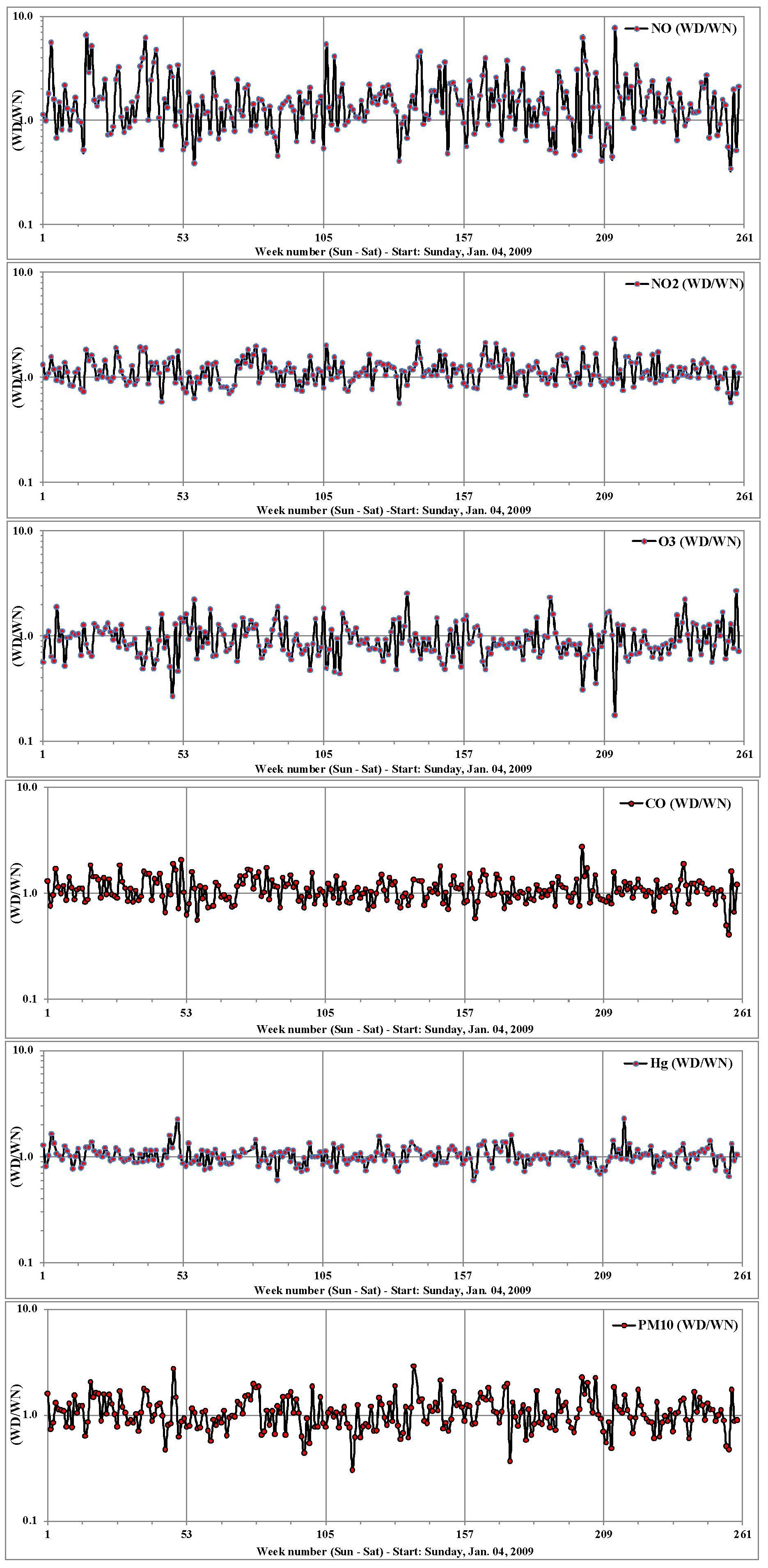
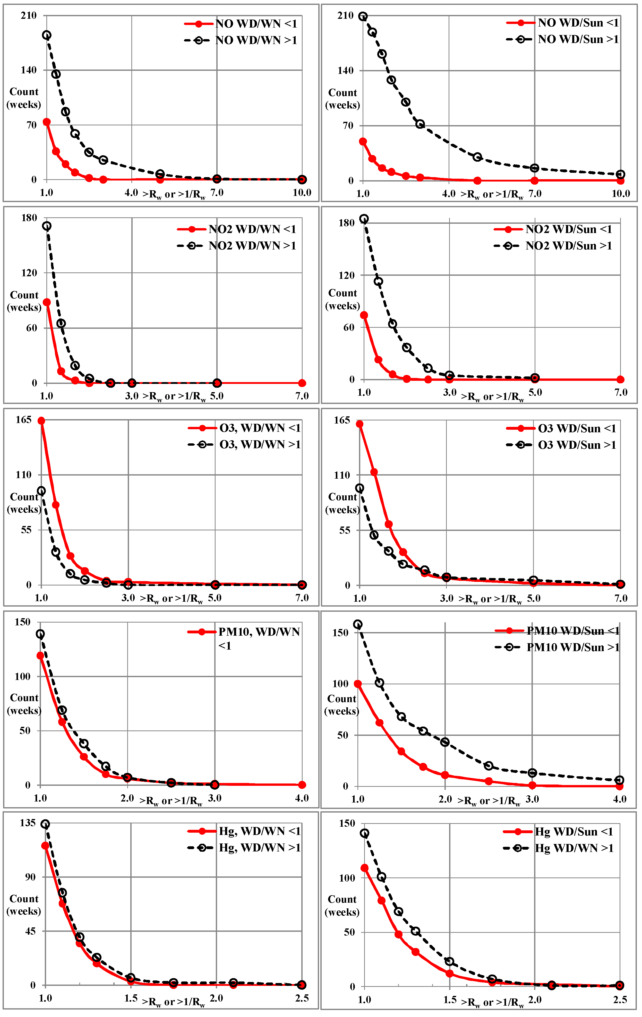
3.1. The Weekday to Weekend (WN/WD and Weekday to Sunday (WD/Sun)) Concentration Ratios (Rw) of NO, NO2 and O3

The WD/WN (or WD/Sun) ratios (Rw) can provide insights on the temporal distribution of air pollutants which may lead to more reliable forecasting of pollutant levels [19,21,35]. Various factors, such as the seasons, traffic density, fuel type and usage and waste disposal activities (specifically, landfills and incineration), may give rise to differences in the WD and WN pollutant levels [21].
To learn more about the WD/WN effects, the results of NO, NO2 and O3 analysis were assessed on multiple temporal scales. In Figure 2, we show the WD/WN trend over the 5-year study period (note that the y-axis scale is logarithmic). The AM (and range) of the WD/WN data for NO, NO2 and O3 were 1.65 (0.34–7.7), 1.17 (0.57–2.31) and 0.96 (0.18–4.12), respectively. The corresponding GM for the WD/WN effect for NO, NO2 and O3 were, 1.38, 1.13 and 0.89, respectively. Out of the Rw values, a large fraction was greater than 1.0 (i.e., NO (71%), NO2 (66%) and O3 (36%)) for the entire 260-week study period. The WD/WN effect (where Rw > 1) was thus clearly distinguished between the pollutant species in a relative order of magnitude as NO > NO2 > O3.
For the entire study period, the average hourly Saturday and Sunday pollution levels were significantly different, for example, NO: 20.5 and 14.3 ppb, respectively (p = 1.77 × 10⁻⁴, two-tailed) and O3: 18.9 and 22.5 ppb, respectively (p = 6.12 × 10⁻⁴, two-tailed). On the other hand, the average WD and Saturday pollution levels were more similar (Table 1). Similar behavior was reported in a study covering the period 1986–2007 in the Mexico City metropolitan area; the peak 3-h NOx levels were 80 (Sun), 137 (WD) and 115 ppb (Sat). Thus, there was a strong WD/Sun effect of 1.72. and the corresponding CO WD/Sun value was 1.61. Both NOx and CO levels peaked around 8–11 a.m. Therein, PM10 and O3 showed smaller WD/Sat or WD/Sun effects [36].
The corresponding AM and GM of the WD/Sun Rw values were respectively, NO (2.73 and 2.01), NO2 (1.41 and 1.29), O3 (1.08 and 0.88), CO (1.22 and 1.15), PM10 (1.35 and 1.07) and Hg (1.08 and 1.04). The ratio of the hourly averaged WD and Sunday pollution data for the entire study period is in better agreement with the GM but not the AM of the WD/Sun Rw values, for example, NO (1.58 vs. 2.01 vs. 2.73), respectively. The presents work’s YS urban site WD/Sun effect GM of 2.01 is comparable to the quantile:quantile analysis estimate of ~2.7 during the photochemical season of May through September of 1972 and 1973 at Elizabeth (an urban area), NJ, USA [28].
The influence of high road traffic density, as well as other transportation and industrial activities, on WD pollutant levels is more pronounced than the mere natural fluctuations at the road curbside [37,38]. From year to year, the NO and NO2 WD/WN effect had shown negligible variation. Since the NO WD/WN pattern for each year is similar to that of NO2, it may imply that O3 plays a key role in the formation of NO2; the most likely pathway is oxidation [15], as shown in Equation (2):
NO + O3 → NO2 + O2
In the presence of UV light (hυ), NO and O3 can be regenerated as shown in Equation (3):
NO2 + O2 + hυ → NO + O3
Several hypotheses for the O3 weekend effect and modeling including the role of volatile organic compounds in NO2 and O3 formation have been discussed in detail elsewhere [36]. According to plots of hourly [NO2] versus hourly [O3] for weeks #73 (starting 23 May 2010) and #212 (starting 20 January 2013), [O3] is the highest at low [NO2] but very low at high [NO2] (Figure S2). A Pearson correlation analysis gave large negative results, viz., −0.800 for week #73 and −0.905 for week # 212. Also shown in Figure S2 are plots of (a) [NO], (b) [NO2], (c) [O3], or (d) [NO2] + [O3] at hourly intervals. Although [NO2] and [O3] individually showed large temporal variations over the two 168 h periods, the sum of [NO2] + [O3] showed much reduced hourly variation; this observation is suspected to reflect an essentially a constant mass scenario in which NO2 and O3 are merely interconverted from one species to the other. These explanations indeed conform to already well-known O3-NOX atmospheric chemistry processes. It would have been of interest to study the effect of ozone precursors, especially volatile organic compounds (VOC), on ozone concentration. Unfortunately, there is not enough detailed information about VOC concentrations (i.e., a photochemical assessment monitoring station (PAMS)) near the monitoring station to allow this analysis. It is worth noting that at another site in Seoul (Jong-ro) equipped with PAMS, both [toluene] and [NO] were a factor up to ~3 higher on WDs compared to Sundays for most weeks [39]. A detailed kinetics study is also beyond the scope of this study.
A large fraction of the NO WD/WN and WD/Sun Rw ratios were >1, contrary to those of the O3; an indication of the influence of parameters other than emissions from vehicles and natural gas heating system. It is commonly believed that the major source of curbside NO is from internal combustion engines and this may be true for April through October (Figure S1) as natural gas use (mainly for building heating purposes) is at its lowest in the warmer months. Nationally, between December 2011 and December 2013, city gas demand ranged from a high of 2924 k·ton in January 2013 (average monthly temperature = −3.2 °C) to a low of 917 k·ton in September 2013 (average monthly temperature = 21.5 °C (http://www.kesis.net/). The per-capita city gas demand in Yong-san or Seoul is assumed to be very similar to the national per-capita demand. For monthly temperatures between 21–28 °C, the national city gas demand was 949 ± 33 k·ton·month−1; for monthly temperatures below 21 °C, national demand followed this relationship: =6.08 × 10⁶/(273 + T) − 19,800 k·ton·month−1 (p = 0.991) where T (−3.8 to 20.6 °C) is the monthly temperature in Yong-san). The high NO WD/WN and WD/Sunday effect indicates the possibility that traffic density and industrial activities were at their lowest on weekends and Sundays. However, the estimated NOx emissions from 65,000 cars in Yong-san Gu (assuming 0.08 g·NOx·km−1 (Euro-4 standard, gasoline) and 37 km·day−1) is only 70 ton·yr−1 compared to total NOx emissions of ~1500 ton·yr−1 in Yong-san Gu (URL: http://airemiss.nier.go.kr/mbshome/mbs/airemiss/index.do (in Korean)). In South Korea, the monthly consumption of gasoline (~1000 k·ton·month−1) and diesel (~2000 k·ton·month−1) has been very stable over the period May 2011 to April 2017 unlike city gas demand (KESIS, URL: http://www.kesis.net/). Thus, the major NO and CO emission sources are suspected to be from the combustion of city natural gas in the colder months of the year.

3.2. Influence of Meteorological Parameters on Weekday/Sunday Effect (Rw) for NO, NO2, O3 and CO

Based on our previous work [30], we attempted to identify whether one or more meteorological parameters are correlated with the observed WD/Sunday profiles. Table S2 summarizes the Pearson correlation analysis data for selected pollutants versus Sunday temperature, UV, wind speed, relative humidity and solar irradiance data. In general, the meteorological parameters had very little positive influence on Rw values, for example, for NO, the Rw:temperature, r = −0.08. and O3, the Rw:temperature, r = −0.04. The strongest positive influence was seen for wind speed, NO2:Wind (r = 0.45), NO:Wind (r = 0.34) and CO:Wind (r = 0.35) and that for O3:Wind was negative (r = −0.35). This is possibly because higher wind speed ensures better dispersal mixing of the air in the tropopause. There was, however, some modest negative influence; for example, O3 (Rw):UV, r = −0.29 unlike the daily concentration data where the correlation is strongly positive, [O3]:UV, r = 0.65 thus some apparent inconsistencies exist for unknown reasons.

3.3. PM10 and Hg WD/WN Effect

Airborne mercury is also of interest because it has different source to many of the other pollutants examined. Because no weekday/weekend effect was observed, we can conclude that the sources are not the same as the other pollutants for which a weekday/weekend effect. This indicates that in this location in Seoul, mercury is mostly a background pollutant with most contributions from background levels and long-term transport and not heavily influenced by local emissions. PM10 shows minimal WD/WN or WD/Sun effect again suggesting the NO and PM10 emissions are from different and unrelated sources.

3.4. Other Studies on the WD/WN Effect

Although 16 similar studies on the WD/WN effect were published from 1995 to 2014 [15,16,17,18,19,20,21,35,36,40,41,42,43,44,45], our current work has identified a strong relationship (and interdependence) between the NO, NO2, O3 and CO WD/WN and WD/Sun effect and the meteorological parameters. Of the aforementioned 16 references, it was noted that the concentrations of specific air pollutants (i.e., SO2, NOx and PM10) are nearly constant on weekdays (WD) but were approximately 40–60% lower on weekends (WN) in southwestern Germany [46]. Prior to this, Mayer had established the differences between weekday and weekend levels of NO, NO2 and O3, as well as other air pollutants that were routinely monitored for temporal variability, at an official air-quality monitoring station in the Bad Cannstatt district of Stuttgart between 1981 and 1993 [47]. The WD/WN effect was strongly influenced by motor traffic in Stuttgart, a large city in southern Germany with a population of approximately 500,000. More recently, the diurnal NOx levels were found to exhibit two peaks during weekdays at 6–8 am and 4–8 pm, which were attributed to rush-hour traffic [17]. During weekends, only a single, afternoon peak was observed, which can be attributed to higher rates of leisure activities.

4. Conclusions

We investigated for evidence of the weekday/weekend (WD/WN) and weekday/Sunday (WD/Sun) effects of pollution levels based on the temporal distribution of NO, NO2, O3 and CO at an urban (Yong-San) air-quality monitoring station in the Seoul megalopolis. The data strongly indicate that the NO WD/WN and WD/Sunday ratios may be due in part of lower NO emissions (reduced diesel vehicle movements and natural gas use) on Saturdays and Sundays relative to weekdays. The weekly NO and O3 levels have a poor Pearson correlation (r = −0.60) and there is a ~6-month phase difference between NO and O3 minima and maxima. On the other hand, the NO:City gas use pair has the highest Pearson correlation of r = 0.82 of all such studied pairs. There were no unexpected observations with regard to the intra- or inter-year level, WD/WN or WD·Sun (Rw) ratio for each pollutant. The geometric mean of the WD/Sun (or WD/WN) weekly effect and the hourly averaged pollution data (weekday, Saturday and Sunday) is the most reliable means to determine the existence of any WD/Sun or WD/WN effect; the arithmetic mean is the least reliable and therefore strongly discouraged. We plan to examine other sites throughout South Korea for the spatial distribution of oxides of nitrogen, ozone and particulate matters in the future, over a decade. Based on our study, it is recommended that the political decision makers should implement policies to reduce pollutant emissions more effectively during weekdays from major man-made sources in the Republic of Korea. If total NO emissions are reduced, then airborne [NO], [NO2] and [O3] should all decrease as they are coupled through chemical reactions.

Supplementary Materials

The following are available online at https://www.mdpi.com/2071-1050/10/4/1248/s1. Table S1. Basic information regarding instrumentation used for measuring three target pollutants (NO, NO2 and O3) and meteorological data; Table S2. Number of weeks that the Weekday/Sunday effect ratio (Rw or >1/Rw) is greater than a selected value (always ≥1) for NO, NO2, O3, Hg and PM10 using the Microsoft Excel COUNTIF facility; Table S3. Pearson correlation analysis of the daily mean data, Weekday/Sunday effect (Rw) for NO, NO2, O3 and CO with selected meteorological data and monthly data (NO, CO, temperature and city gas demand; Figure S1. The mean weekday (Monday through Friday) [NO] (top panel) versus mean Sunday [NO] levels (middle panel) for each week. The bottom panel shows the weekday/Sun effect (Rw) of NO for each week; Figure S2. Plots of [NO2] versus [O3] and [NO], [NO2], [O3] or [NO2] + [O3] at every hour for weeks #73 (WD/Sunday effect = 12.0) and #212 (WD/Sunday effect = 0.27).

Acknowledgments

The authors acknowledge support from a National Research Foundation of Korea (NRF) grant funded by the Ministry of Science, ICT and Future Planning (No. 2016R1E1A1A01940995). K.-H.K. also acknowledges support made by the Korea Ministry of Environment (MOE) (2015001950001) as part of “The Chemical Accident Prevention Technology Development Project.”

Author Contributions

Initially, A.A.A. analyzed the data, conducted the literature survey, drafted the main manuscript text and prepared the Tables and Figures. Later, J.E.S. re-analyzed the data, conducted a literature survey and made major revisions to the manuscript text, Tables and Figures. J.E.S. (assistant principal investigator) and K.-H.K. (principal investigator) reviewed and edited the draft manuscript for scientific content. In addition, J.E.S. and K.-H.K. performed the overall internal review (with assistance from the other authors, viz., J.W.S., K.V., E.-C.J., J.H. and R.J.C.B.).

Conflicts of Interest

The authors declare no conflict of interest.

References

  1. USEPA. National Emissions Inventory. Available online: https://www.epa.gov/air-emissions-inventories (accessed on 18 March 2017).
  2. Lewne, M.; Cyrys, J.; Meliefste, K.; Hoek, G.; Brauer, M.; Fischer, P.; Gehring, U.; Heinrich, J.; Brunekreef, B.; Bellander, T. Spatial variation in nitrogen dioxide in three European areas. Sci. Total Environ. 2004, 332, 217–230. [Google Scholar] [CrossRef] [PubMed]
  3. Barck, C.; Lundahl, J.; Hallden, G.; Bylin, G. Brief exposures to NO2 augment the allergic inflammation in asthmatics. Environ. Res. 2005, 97, 58–66. [Google Scholar] [CrossRef] [PubMed]
  4. Carslaw, D.C. Evidence of an increasing NO2/NOx emissions ratio from road traffic emissions. Atmos. Environ. 2005, 39, 4793–4802. [Google Scholar] [CrossRef]
  5. Carslaw, D.C.; Beevers, S.D. Investigating the potential importance of primary NO2 emissions in a street canyon. Atmos. Environ. 2004, 38, 3585–3594. [Google Scholar] [CrossRef]
  6. Carslaw, D.C.; Beevers, S.D. New Directions: Should road vehicle emissions legislation consider primary NO2? Atmos. Environ. 2004, 38, 1233–1234. [Google Scholar] [CrossRef]
  7. Chai, F.H.; Gao, J.; Chen, Z.X.; Wang, S.L.; Zhang, Y.C.; Zhang, J.Q.; Zhang, H.F.; Yun, Y.R.; Ren, C. Spatial and temporal variation of particulate matter and gaseous pollutants in 26 cities in China. J. Environ. Sci.-China 2014, 26, 75–82. [Google Scholar] [CrossRef]
  8. Bytnerowicz, A.; Omasa, K.; Paoletti, E. Integrated effects of air pollution and climate change on forests: A northern hemisphere perspective. Environ. Pollut. 2007, 147, 438–445. [Google Scholar] [CrossRef] [PubMed]
  9. Derwent, R.G.; Hertel, O. Transformation of Air Pollutants (Urban Air Pollution-European Aspects); Kluwer Academic Publishers: Dordrecht, The Netherlands, 1998. [Google Scholar]
  10. Seinfeld, J.H.; Pandis, S.N. Atmospheric Chemistry And Physics—From Air Pollution to Climate Change, 2nd ed.; John Wiley & Sons, Inc.: Hoboken, NJ, USA, 2006. [Google Scholar]
  11. Nishanth, T.; Praseed, K.M.; Kumar, M.K.S.; Valsaraj, K.T. Observational Study of Surface O3, NOx, CH4 and Total NMHCs at Kannur, India. Aerosol Air Qual. Res. 2014, 14, 1074–1088. [Google Scholar] [CrossRef]
  12. Sahu, L.K.; Saxena, P. High time and mass resolved PTR-TOF-MS measurements of VOCs at an urban site of India during winter: Role of anthropogenic, biomass burning, biogenic and photochemical sources. Atmos. Res. 2015, 164, 84–94. [Google Scholar] [CrossRef]
  13. Sahu, L.K.; Yadav, R.; Pal, D. Source identification of VOCs at an urban site of western India: Effect of marathon events and anthropogenic emissions. J. Geophys. Res.-Atmos. 2016, 121, 2416–2433. [Google Scholar] [CrossRef]
  14. Alghamdi, M.A.; Khoder, M.; Harrison, R.M.; Hyvarinen, A.P.; Hussein, T.; Al-Jeelani, H.; Abdelmaksoud, A.S.; Goknil, M.H.; Shabbaj, I.I.; Almehmadi, F.M.; et al. Temporal variations of O3 and NOx in the urban background atmosphere of the coastal city Jeddah, Saudi Arabia. Atmos. Environ. 2014, 94, 205–214. [Google Scholar] [CrossRef]
  15. Huryn, S.M.; Gough, W.A. Impact of urbanization on the ozone weekday/weekend effect in Southern Ontario, Canada. Urban Clim. 2014, 8, 11–20. [Google Scholar] [CrossRef]
  16. Kim, B.G.; Choi, M.H.; Ho, C.H. Weekly periodicities of meteorological variables and their possible association with aerosols in Korea. Atmos. Environ. 2009, 43, 6058–6065. [Google Scholar] [CrossRef]
  17. Melkonyan, A.; Kuttler, W. Long-term analysis of NO, NO2 and O3 concentrations in North Rhine-Westphalia, Germany. Atmos. Environ. 2012, 60, 316–326. [Google Scholar] [CrossRef]
  18. Porter, W.C.; Khalil, M.A.K.; Butenhoff, C.L.; Almazroui, M.; Al-Khalaf, A.K.; Al-Sahafi, M.S. Annual and weekly patterns of ozone and particulate matter in Jeddah, Saudi Arabia. J. Air Waste Manag. 2014, 64, 817–826. [Google Scholar] [CrossRef]
  19. Sadanaga, Y.; Shibata, S.; Hamana, M.; Takenaka, N.; Bandow, H. Weekday/weekend difference of ozone and its precursors in urban areas of Japan, focusing on nitrogen oxides and hydrocarbons. Atmos. Environ. 2008, 42, 4708–4723. [Google Scholar] [CrossRef]
  20. Wang, Y.H.; Hu, B.; Ji, D.S.; Liu, Z.R.; Tang, G.Q.; Xin, J.Y.; Zhang, H.X.; Song, T.; Wang, L.L.; Gao, W.K.; et al. Ozone weekend effects in the Beijing-Tianjin-Hebei metropolitan area, China. Atmos. Chem. Phys. 2014, 14, 2419–2429. [Google Scholar] [CrossRef]
  21. Wolff, G.T.; Kahlbaum, D.F.; Heuss, J.M. The vanishing ozone weekday/weekend effect. J. Air Waste Manag. 2013, 63, 292–299. [Google Scholar] [CrossRef]
  22. Masiol, M.; Agostinelli, C.; Formenton, G.; Tarabotti, E.; Pavoni, B. Thirteen years of air pollution hourly monitoring in a large city: Potential sources, trends, cycles and effects of car-free days. Sci. Total Environ. 2014, 494, 84–96. [Google Scholar] [CrossRef] [PubMed]
  23. Cerveny, R.S.; Balling, R.C. Weekly cycles of air pollutants, precipitation and tropical cyclones in the coastal NW Atlantic region. Nature 1998, 394, 561–563. [Google Scholar] [CrossRef]
  24. Bell, T.L.; Rosenfeld, D.; Kim, K.M.; Yoo, J.M.; Lee, M.I.; Hahnenberger, M. Midweek increase in US summer rain and storm heights suggests air pollution invigorates rainstorms. J. Geophys. Res.-Atmos. 2008. [Google Scholar] [CrossRef]
  25. Tuttle, J.D.; Carbone, R.E. Inferences of weekly cycles in summertime rainfall. J. Geophys. Res.-Atmos. 2011. [Google Scholar] [CrossRef]
  26. Henschel, S.; Le Tertre, A.; Atkinson, R.W.; Querol, X.; Pandolfi, M.; Zeka, A.; Haluza, D.; Analitis, A.; Katsouyanni, K.; Bouland, C.; et al. Trends of nitrogen oxides in ambient air in nine European cities between 1999 and 2010. Atmos. Environ. 2015, 117, 234–241. [Google Scholar] [CrossRef]
  27. Baidar, S.; Hardesty, R.M.; Kim, S.W.; Langford, A.O.; Oetjen, H.; Senff, C.J.; Trainer, M.; Volkamer, R. Weakening of the weekend ozone effect over California’s South Coast Air Basin. Geophys. Res. Lett. 2015, 42, 9457–9464. [Google Scholar] [CrossRef]
  28. Cleveland, W.S.; Graedel, T.E.; Kleiner, B.; Warner, J.L. Sunday and Workday Variations in Photochemical Air-Pollutants in New-Jersey and New-York. Science 1974, 186, 1037–1038. [Google Scholar] [CrossRef] [PubMed]
  29. Gong, D.Y.; Ho, C.H.; Chen, D.L.; Qian, Y.; Choi, Y.S.; Kim, J.W. Weekly cycle of aerosol-meteorology interaction over China. J. Geophys. Res.-Atmos. 2007. [Google Scholar] [CrossRef]
  30. Vellingiri, K.; Kim, K.H.; Jeon, J.Y.; Brown, R.J.C.; Jung, M.C. Changes in NOx and O3 concentrations over a decade at a central urban area of Seoul, Korea. Atmos. Environ. 2015, 112, 116–125. [Google Scholar] [CrossRef]
  31. Kim, K.-H.; Sul, K.-H.; Szulejko, J.E.; Chambers, S.D.; Feng, X.; Lee, M.-H. Progress in the reduction of carbon monoxide levels in major urban areas in Korea. Environ. Pollut. 2015, 207, 420–428. [Google Scholar] [CrossRef] [PubMed]
  32. SODP. Seoul Data Open Plaza. Available online: http://stat.seoul.go.kr/octagonweb/jsp/WWS7/WWSDS7100.jsp (accessed on 18 March 2017).
  33. SMG. Seoul Metropolitan Government. Major traffic statistics. Available online: http://english.seoul.go.kr/policy-information/traffic/major-traffic-statistics/ (accessed on 18 March 2017).
  34. Kim, N.K.; Kim, Y.P.; Morino, Y.; Kurokawa, J.; Ohara, T. Verification of NOx emission inventory over South Korea using sectoral activity data and satellite observation of NO2 vertical column densities. Atmos. Environ. 2013, 77, 496–508. [Google Scholar] [CrossRef]
  35. Qin, Y.; Tonnesen, G.S.; Wang, Z. Weekend/weekday differences of ozone, NOx, CO, VOCs, PM10 and the light scatter during ozone season in southern California. Atmos. Environ. 2004, 38, 3069–3087. [Google Scholar] [CrossRef]
  36. Stephens, S.; Madronich, S.; Wu, F.; Olson, J.B.; Ramos, R.; Retama, A.; Munoz, R. Weekly patterns of Mexico City’s surface concentrations of CO, NOx, PM10 and O3 during 1986–2007. Atmos. Chem. Phys. 2008, 8, 5313–5325. [Google Scholar] [CrossRef]
  37. Tang, G.; Wang, Y.; Li, X.; Ji, D.; Hsu, S.; Gao, X. Spatial-temporal variations in surface ozone in Northern China as observed during 2009–2010 and possible implications for future air quality control strategies. Atmos. Chem. Phys. 2012, 12, 2757–2776. [Google Scholar] [CrossRef]
  38. Wang, T.; Nie, W.; Gao, J.; Xue, L.K.; Gao, X.M.; Wang, X.F.; Qiu, J.; Poon, C.N.; Meinardi, S.; Blake, D.; et al. Air quality during the 2008 Beijing Olympics: Secondary pollutants and regional impact. Atmos. Chem. Phys. 2010, 10, 7603–7615. [Google Scholar] [CrossRef]
  39. Khan, A.; Szulejko, J.E.; Kim, K.-H.; Brown, R.J.C. Airborne volatile aromatic hydrocarbons at an urban monitoring station in Korea from 2013 to 2015. J. Environ. Manag. 2018, 209, 525–538. [Google Scholar] [CrossRef] [PubMed]
  40. Altshuler, S.L.; Arcado, T.D.; Lawson, D.R. Weekday vs. Weekend Ambient Ozone Concentrations—Discussion and Hypotheses with Focus on Northern California. J. Air Waste Manag. 1995, 45, 967–972. [Google Scholar] [CrossRef]
  41. Baumer, D.; Vogel, B. An unexpected pattern of distinct weekly periodicities in climatological variables in Germany. Geophys. Res. Lett. 2007, 34, L03819. [Google Scholar] [CrossRef]
  42. Henschel, S.; Querol, X.; Atkinson, R.; Pandolfi, M.; Zeka, A.; Le Tertre, A.; Analitis, A.; Katsouyanni, K.; Chanel, O.; Pascal, M.; et al. Ambient air SO2 patterns in 6 European cities. Atmos. Environ. 2013, 79, 236–247. [Google Scholar] [CrossRef]
  43. Heuss, J.M.; Kahlbaum, D.F.; Wolff, G.T. Weekday/weekend ozone differences: What can we learn from them? J. Air Waste Manag. 2003, 53, 772–788. [Google Scholar] [CrossRef]
  44. Marr, L.C.; Harley, R.A. Spectral analysis of weekday-weekend differences in ambient ozone, nitrogen oxide, and non-methane hydrocarbon time series in California. Atmos. Environ. 2002, 36, 2327–2335. [Google Scholar] [CrossRef]
  45. Shutters, S.T.; Balling, R.C. Weekly periodicity of environmental variables in Phoenix, Arizona. Atmos. Environ. 2006, 40, 304–310. [Google Scholar] [CrossRef]
  46. Baumer, D.; Rinke, R.; Vogel, B. Weekly periodicities of Aerosol Optical Thickness over Central Europe—Evidence of an anthropogenic direct aerosol effect. Atmos. Chem. Phys. 2008, 8, 83–90. [Google Scholar] [CrossRef]
  47. Mayer, H. Air pollution in cities. Atmos. Environ. 1999, 33, 4029–4037. [Google Scholar] [CrossRef]
Figure 1. Comparison of the weekday-weekend ratio (Rw) plots (at weekly intervals) of NO, NO2, O3, CO, Hg and PM10 from 2009 to 2013. Note: The y-axis scale is logarithmic to gauge whether the distribution is symmetrical with respect to the y = 1 line.
Sustainability 10 01248 g001
Figure 2. Number of weeks that the Weekday/Weekend or Weekday/Sunday effect ratio (Rw or 1/Rw) is greater than a selected value (always ≥1) for NO, NO2, O3, Hg and PM10.
Sustainability 10 01248 g002
Table 1. Summary of airborne pollutant WD/WN and WD/Sun effect and meteorological data at Yong-San, Seoul, Korea (2009–2013): (a) air pollutant (WD/WN) effect, (b) air pollutant (WD/Sun) effect) and (c) meteorological (WD–WN) effect.
ItemSpeciesAll Hourly Data AverageWeekdays aWeekend a(WD–WN)UnitsWD/WNWD/WNWD/WN%t-TestHourly Data Coverage (%)Strength of
(MTWTF)(Sat, Sun)Difference RwRwppb Ratioof Rwp ValueWD/Sun Effect
WDWN (AM) b(GM) c >1.00WD:WN
(a)NO21.1 ± 21.422.6 ± 16.817.3 ± 14.75.3(ppb)1.651.381.3071.41.83 × 10−499.1Strong
NO236.1 ± 13.537.3 ± 10.033.4 ± 10.13.9(ppb)1.171.131.1266.01.16 × 10−599.1Moderate
O319.1 ± 11.118.4 ± 8.720.7 ± 9.9−2.3(ppb)0.960.890.8936.34.70 × 10−399.0Moderate inverse
CO527 ± 279534 ± 241504 ± 23430(ppb)1.101.061.0659.00.16199.0Weak
PM1047.7 ± 30.347.9 ± 21.447.3 ± 24.00.6(µg·m−3)1.091.031.0153.70.77999.0Very weak
Hg3.1 ± 1.33.1 ± 1.23.0 ± 1.00.1(ng·m−3)1.031.011.0251.40.47198.8No evidence
(b) SunWDSatWD-Sun WD/SunWD/SunWD/Sun Sat:Sun
(AM)(GM)ppb ratio t-test
NO14.3 ± 16.622.6 ± 16.820.5 ± 20.88.3(ppb)2.732.011.5880.71.77 × 10−4-Strong
NO230.6 ± 12.737.3 ± 10.036.2 ± 12.76.7(ppb)1.411.291.2271.41.15 × 10−6-Moderate
O322.5 ± 12.618.4 ± 8.718.9 ± 10.9−4.1(ppb)1.080.880.8237.66.12 × 10−4-Moderate inverse
CO488 ± 276534 ± 241520 ± 27446(ppm)1.221.151.0968.40.185-Weak-moderate
PM1044.9 ± 28.647.9 ± 21.449.7 ± 33.53.0(µg·m−3)1.351.071.0761.20.085-Weak
Hg3.0 ± 1.23.1 ± 1.33.0 ± 1.20.1(ng·m−3)1.081.041.0356.40.871-No evidence
ParameterAll hourlyWeekdaysWeekend(WD–WN)Units % of Strength of
data(MTWTF)(Sat, Sun)difference (WD-Sun) WD/Sun effect
averageWDWN >0.0
(c)Wind speed2.5 ± 0.62.5 ± 0.42.5 ± 0.40.0(m·s−1)---54.1-99.4No evidence
Temperature12.6 ± 10.812.6 ± 10.612.7 ± 10.5−0.1(°C)---49.4-99.8No evidence
Relative humidity58.6 ± 1458.5 ± 1159.1 ± 11−0.6(%)---45.6-99.8No evidence
UV3.8 ± 2.03.8 ± 1.63.8 ± 1.70.0(W·m−2)---47.5-99.4No evidence
Solar radiance143.6 ± 78143.8 ± 54143.4 ± 610.4(W·m−2)---50.6-99.4No evidence
a A week is defined as Sunday through Saturday. For each week, weekdays (WD) are defined as Monday through Friday and the weekend (WN) is defined as Sunday (first day) and Saturday (last day); b AM—arithmetic mean; c GM—geometric mean.

