Coseismic Fault Model of Mw 8.3 2015 Illapel Earthquake (Chile) Retrieved from Multi-Orbit Sentinel1-A DInSAR Measurements

Abstract

On 16 September 2015, a Mw 8.3 interplate thrust earthquake ruptured offshore the Illapel region (Chile). Here, we perform coseismic slip fault modeling based on multi-orbit Sentinel 1-A (S1A) data. To do this, we generate ascending and descending S1A interferograms, whose combination allows us to retrieve the EW and vertical components of deformation. In particular, the EW displacement map highlights a westward displacement of about 210 cm, while the vertical map shows an uplift of about 25 cm along the coast, surrounded by a subsidence of about 20 cm. Following this analysis, we jointly invert the multi-orbit S1A interferograms by using an analytical approach to search for the coseismic fault parameters and related slip values. Most of the slip occurs northwest of the epicenter, with a maximum located in the shallowest 20 km. Finally, we refine our modeling approach by exploiting the Finite Element method, which allows us to take geological and structural complexities into account to simulate the slip along the slab curvature, the von Mises stress distribution, and the principal stress axes orientation. The von Mises stress distribution shows a close similarity to the depth distribution of the aftershock hypocenters. Likewise, the maximum principal stress orientation highlights a compressive regime in correspondence of the deeper portion of the slab and an extensional regime at its shallower segment; these findings are supported by seismological data.

1. Introduction

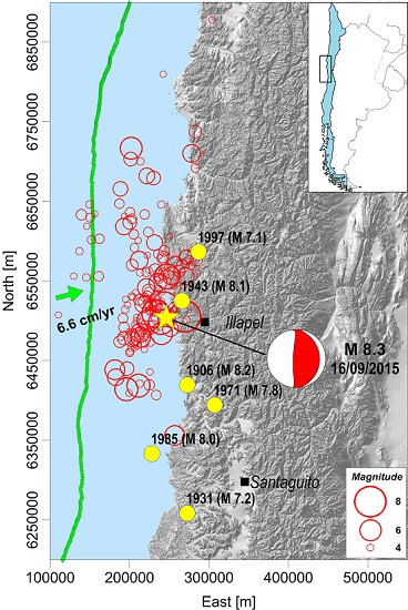
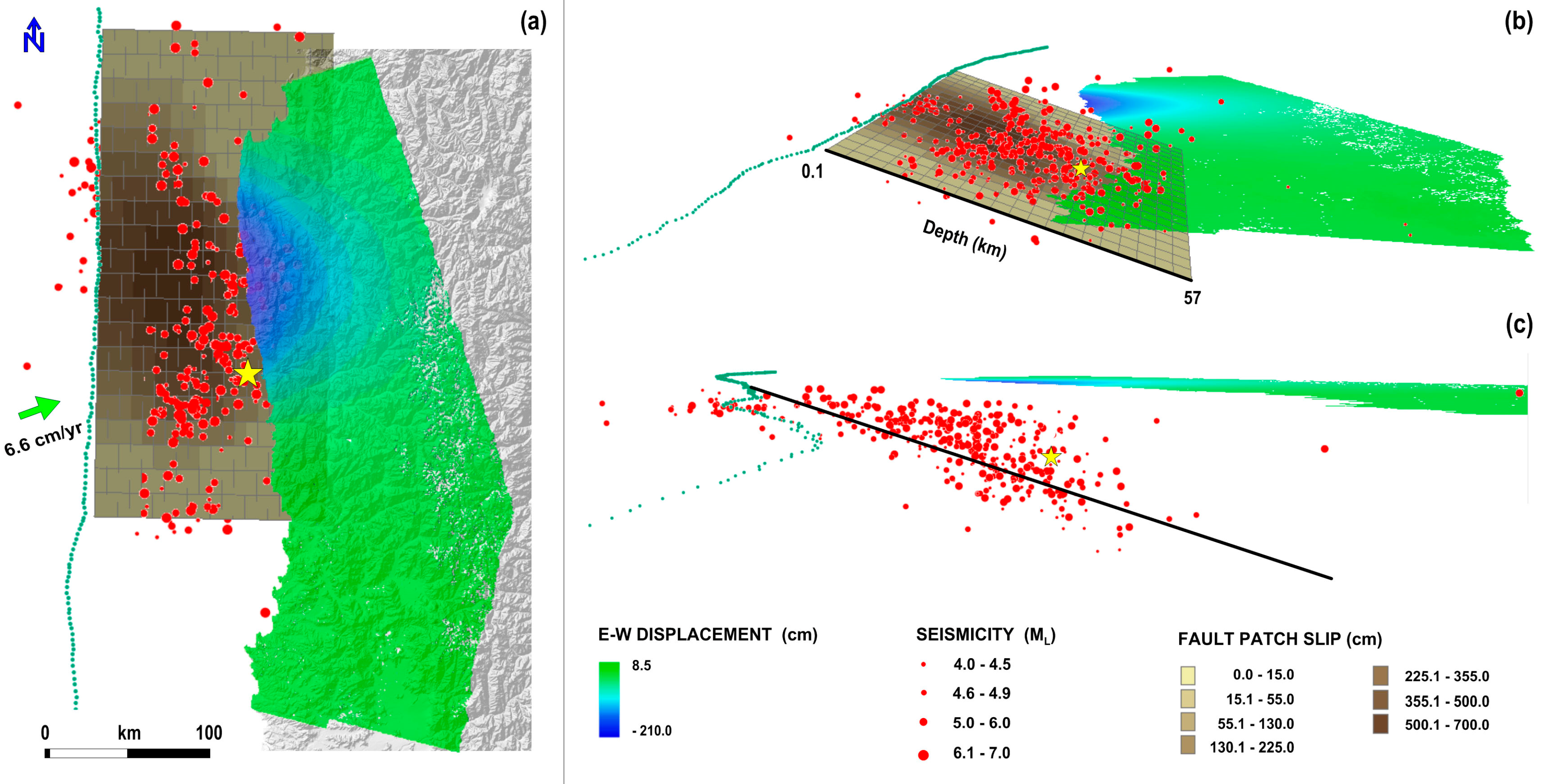
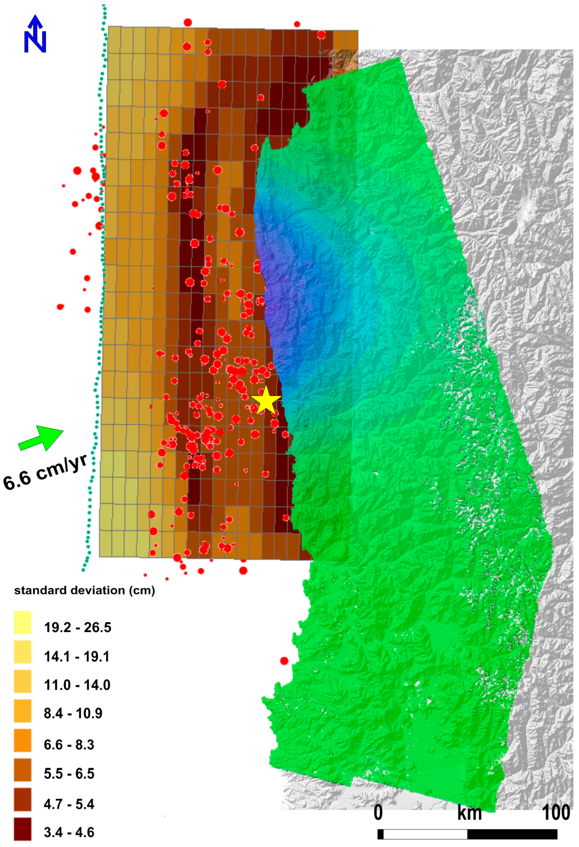
On 16 September 2015, at 22:54 UTC, an earthquake of Mw 8.3, at a depth of 25 km, occurred off the coast of Central Chile in Coquimbo area. The epicenter, located 46 km west of Illapel city (Figure 1), shook buildings in the capital city of Santiago and generated a tsunami that caused flooding in some coastal areas, such as the coastal town of Coquimbo, NW of Illapel, which were hit by waves up to 11 m high after the earthquake [1]. It has been estimated that more than 27,000 people were exposed to severe shaking from this earthquake [USGS PAGER].

The focal mechanism relevant to the main shock, calculated by USGS [2], indicates a N 4° striking sub-horizontal thrust fault. This rupture mechanism is in accordance with the convergence of the Nazca plate toward South American plate at an overall rate of about 6.6 cm/yr [1] (Figure 1). In the first hours, after the main shock event, there were 17 aftershocks in the same area with the strongest one having Mw 7.2 (16 September, 23:18 UTC); most of these aftershocks reveal the same rupture mechanism.

The main event is categorized as an interplate subduction earthquake, localized at the interface between the subducting Nazca and overriding South American plates, supported also by a shallow depth (<50 km) and a nodal plane dipping with a low angle to the East. The South American subduction zone hosted a significant number of large earthquakes that provide details on strain accumulation and release during the earthquake cycle; another key feature of this tectonic setting is the trench-parallel variation in overriding plate shortening, which is maximum in the center and progressively decreases to the North and South [3]. Since 1900, numerous M 7 or larger earthquakes have occurred in this subduction zone (see Figure 1).

We remark that the 2015 Illapel earthquake occurs within the rupture zone of the 1943 M 8.1 seismic event. Since then, after many years of quiescence, the seismic activity of this plate interface suddenly increased in 1997; indeed, 7 events with M > 6 occurred between July 1997 and January 1998 along this shallow dipping subduction zone [4]. During this period, the rupture zone followed a cascade pattern propagating toward the location of the 15 October 1997 M 7.1 earthquake, which occurred at a depth of 68 km [5].

Recently, based on teleseismic data, Ye et al. [6] found that the Illapel earthquake occurred on a bilateral along-strike rupture zone with a larger slip north-northwest of the epicenter, with a peak slip of 7–10 m [6]; Tilmann et al. [7] determined a comprehensive rupture model through the inversion of seismic, GPS, and Sentinel 1-A (S1A) descending data; Melgar et al. [1] resolved a kinematic slip model by using GPS, strong motion and S1A descending and ascending data and jointly analyzed them with teleseismic backprojection. Grandin et al. [8] retrieved the full 3D displacement field by using S1A ascending and descending data, by jointly exploiting the surface deformation measurements components in the across image and the along-track satellite direction, retrieved through the DInSAR and Multiple Aperture Insar (MAI) techniques, respectively.

In this work, a detailed coseismic slip fault model is presented, obtained by taking advantage of the wide spatial coverage and reduced revisit time offered by multi-orbit S1A data, as well as of the high-accuracy measurement capability of the DInSAR technique. In particular, we proceed taking the following three steps: (1) we generate two S1A interferograms for both ascending and descending orbits, respectively, encompassing the main shock, in order to combine the displacements along the satellite Line Of Sight (LOS) for retrieving the EW and vertical components of deformation; (2) we jointly invert multi-orbit S1A deformation LOS measurements by using an analytical approach to search for the coseismic fault parameters; (3) we refine our modeling approach by exploiting the Finite Element (FE) method, which allows us to take into account geological and structural complexities of the region, and to simulate the slip along the subducted slab, the stress distribution, and the principal stress axes orientation.

2. Satellite Data

The used dataset consists of four SAR acquisitions that were taken on 26 August 2015 and 19 September 2015 along ascending orbits (Track 18), and 31 July 2015 and 17 September 2015 over descending ones (Track 156), by the C-Band S1A sensor acquiring data with the Terrain Observation with Progressive Scans (TOPS) mode, which is specifically designed for interferometric application and guarantees a very large spatial coverage [9]. Note that, similar to the ScanSAR, TOPS mode is burst-based; indeed, during the acquisition time, the antenna beam is switched cyclically among different sub-swaths, allowing a significant improvement of the range coverage, but with the detriment of the azimuth resolution. In particular, our SAR data are acquired through the Interferometric Wide Swath (IWS) TOPS mode configuration which is characterized by a swath extension of about 250 km [10]. Such an acquisition mode happens to be particularly effective in the framework of a very large area deformation analysis, as in the case of the Illapel earthquake, at the expense of a coarse spatial resolution (about 15 m and 4 m along azimuth and range, respectively). In our analysis, we jointly process 4 and 3 S1A slices for ascending and descending tracks, respectively, which correspond to an area of ~130,000 km².

By exploiting the available S1A Single Look Complex (SLC) images, we generate two DInSAR interferograms (characterized by a spatial baseline of 75 m and 7 m for ascending and descending orbits, respectively), following a burst-by-burst processing approach and working in radar coordinates (see Figure A1). In particular, we first co-register the SLC bursts through the use of precise orbits information and a 3-arcsec Shuttle Radar Topography Mission (SRTM) DEM of the investigated area [11]. Then, we calculate the DInSAR interferograms for each burst, by using the same DEM for the topographic residue component removal, with a multilook factor of 2 and 10 pixels along the azimuth direction and range, respectively. Subsequently, we compensate for the residual azimuth phase ramp due to possible azimuth mis-registration, through the Enhanced Spectral Diversity method [12] applied to the overlapping areas across consecutive bursts, both on azimuth and range directions. Finally, the compensated wrapped phases of each burst are combined into a single DInSAR interferogram to which the phase unwrapping [13], and the geocoding steps are then applied. Note that, for what concerns the phase unwrapping operation, which permits the retrieval of the interferometric phase (unwrapped interferogram) from its restriction to the [−π, π] interval (wrapped interferogram), it is generally carried out by properly integrating the interferometric phase gradient directly estimated from the wrapped interferogram [14]. Because of the above mentioned integration step, the unwrapped interferogram is available only for the phase of one pixel. This pixel, usually referred to as a reference point, is typically located in a stable area, and its interferometric phase is set to zero (corresponding to the absence of deformation).

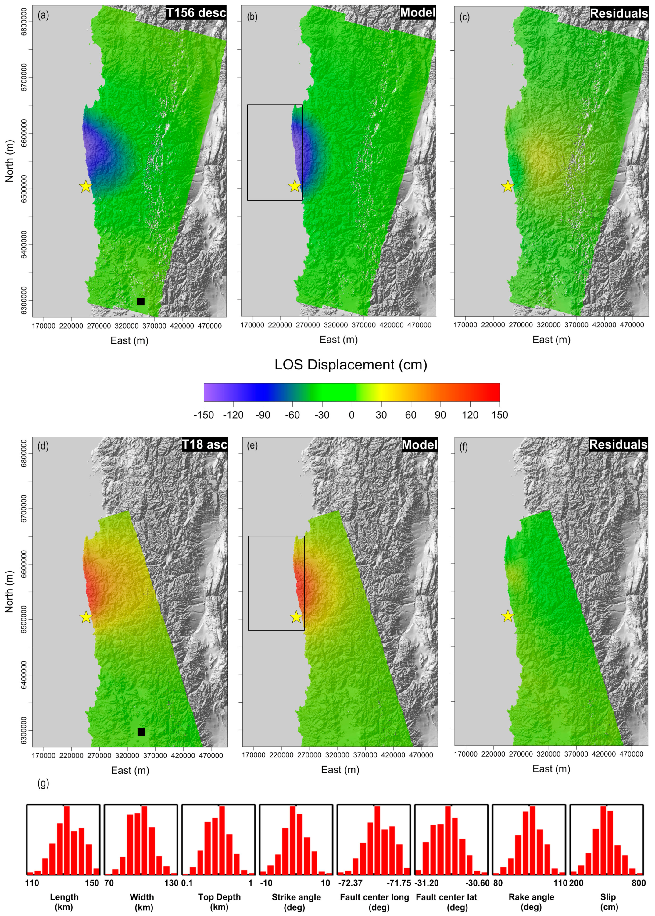
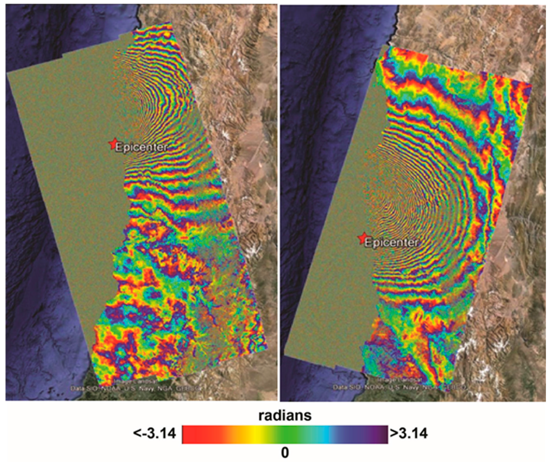
The so-generated coseismic DInSAR deformation maps are presented in Figure 2a,b and exhibit in both cases one main deformation lobe. Moreover, as clearly shown in Figure 2a,b, no phase ramps are present in the resulting interferograms. Such a result is also evident from the analysis of wrapped interferograms, provided in the Appendix (see Figure A1).

In particular, the descending track shows negative LOS displacement values down to −146 cm, corresponding to a sensor-target range increase, while the ascending is characterized by positive values up to ~150 cm, indicating a decrease of the sensor-target distance; the ascending and descending LOS deformation maps reveal that the displacement is almost equal in magnitude and opposite in sign. 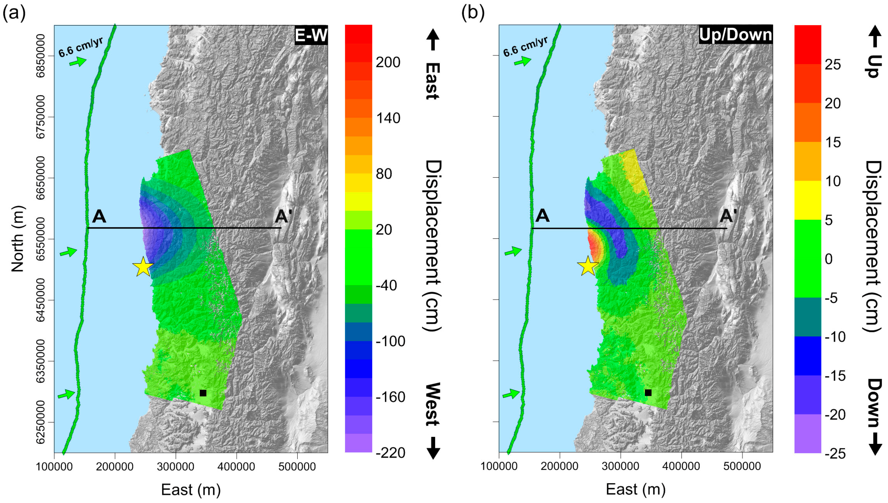These displacement values are in agreement with other works carried out with S1A data to study the Illapel earthquake [8], so phase unwrapping errors can be neglected. Accordingly, the main source of displacement uncertainty is mostly related to atmospheric artefacts, which can be considered in the order of a few phase fringes with a local extension, thus not significantly impacting the retrieved deformation signal induced by the main shock. The availability of both ascending and descending SAR data set allows us not only to detect the ground deformation in the corresponding LOS, but also to discriminate the vertical and east–west components of the displacement [15]. To achieve this task, we properly combine the geocoded displacement maps computed from the ascending and descending orbits on pixels common to both maps, taking into account the different acquisition geometries at each pixel [15,16]. Following the previous discussion, we present in Figure 3a,b the achieved east–west and vertical displacement maps, respectively, evaluated with respect to a pixel identified with a black square in Figure 3a. The east–west displacement map, shown in Figure 3a, clearly highlights a huge displacement to the west of more than 210 cm, while the vertical displacement map (Figure 3b) shows an uplift of about 25 cm along the coast, surrounded by an annular shaped subsidence of about 20 cm; these findings are consistent with GPS measurements reported in Tilmann et al. [7], which indicate an uplift of the coastline and a westward motion approximately radially towards a point offshore near 31.2° S, and with Grandin et al. [8], which highlight a shift from a coastal subsidence to a coastal uplift at 31.1° S.

3. Analytical Modeling

In order to retrieve the seismogenic fault parameters, we now jointly invert S1A DInSAR ascending and descending data following two main steps: a nonlinear inversion to constrain the fault geometries with uniform slip, followed by a linear inversion to retrieve the slip distribution on the fault plane. The observed data is modeled with a finite dislocation fault in an elastic and homogeneous half-space [17]. We search for 8 fault parameters by using a nonlinear inversion algorithm which is based on the Levenberg-Marquardt (LM) least-squares approach, a combination of a gradient descent and Gauss-Newton iteration [18]. Our implementation of the LM is modified with multiple random restarts to guarantee the catching of the global minimum in the optimization process. The dip angle is fixed at 22°, constrained by the aftershock spatial distribution and CGMT fault solution. The cost function is a weighted mean of the residuals, expressed as:

$$CF=\sqrt{\frac{1}{N}{\displaystyle \sum }_i^N\frac{{\left(d_{i,obs}-d_{i,mod}\right)}^2}{{\sigma }_i}}$$

where d_i,obs and d_i,mod are the observed and modeled displacement of the i-th point, and σ_i is the standard deviation for the N points. The DInSAR data is sub-sampled through a QuadTree algorithm [19] over a mesh of about 17,200 points for the descending pass and 25,000 points for the ascending one.

The best fit solution consists of a reverse fault, whose parameters are summarized in

Table 1. Analytical fault model parameters retrieved through non-linear inversion, with the relative standard deviation in parentheses.

Length (km)	Width (km)	Top Depth (km)	Strike (deg)	Dip (deg)	Rake (deg)	Lat (°)	Lon (°)	Average Slip (cm)
170 (0.4)	100 (0.7)	0.1 (0.1)	1 (2)	22 (1)	92 (2)	31.015S (0.01)	72.033W (0.01)	400 (15)

.

The modeled displacement maps (Figure 2c,d) show a good fit with the measured DInSAR data (Figure 2a,b), as highlighted by the residual maps in Figure 2e,f, where the residuals are generally below 25 cm. Figure 2g reports the uncertainty analysis for this non-linear inversion. Some residual deformation is still observed near the main rupture area, which perhaps mainly relates to some local deformation or a more complex geometry of the rupture plane. In order to have a more accurate estimate of the slip along the fault plane, a distributed slip on 20 × 20 patches (with dimensions of 15 × 7.5 km²) is calculated. To this aim, a linear inversion is performed by fixing the parameters of the non-linear inversion (Table 1) and inverting the following system:

$$\left[\begin{array}{c}{d}_{InSAR}\\ 0\end{array}\right]=\left[\begin{array}{c}G\\ k•{\nabla }^2\end{array}\right]•\left[\begin{array}{c}m\\ 0\end{array}\right]$$

where d_InSAR is the InSAR data vector, m is the vector of slip values, G is the Green’s matrix with the point-source functions, and ${\nabla }^2$ is a smoothing Laplacian operator weighted by an empirical coefficient k. The system solution is obtained by means of the Singular Value Decomposition technique of the kernel matrix. In this case, we find a maximum slip of about 7 m in the shallowest 20 km (Figure 4a,b); the RMS for this solution is about 4.6 cm. The standard deviation slip for each patch is reported in Figure A2. The fault length and width are extended to consider the border effects as negligible. Note that most of the aftershocks do not take place close to the areas with a larger slip, but they occur in their surroundings; this finding is very similar to what was found by USGS [20].

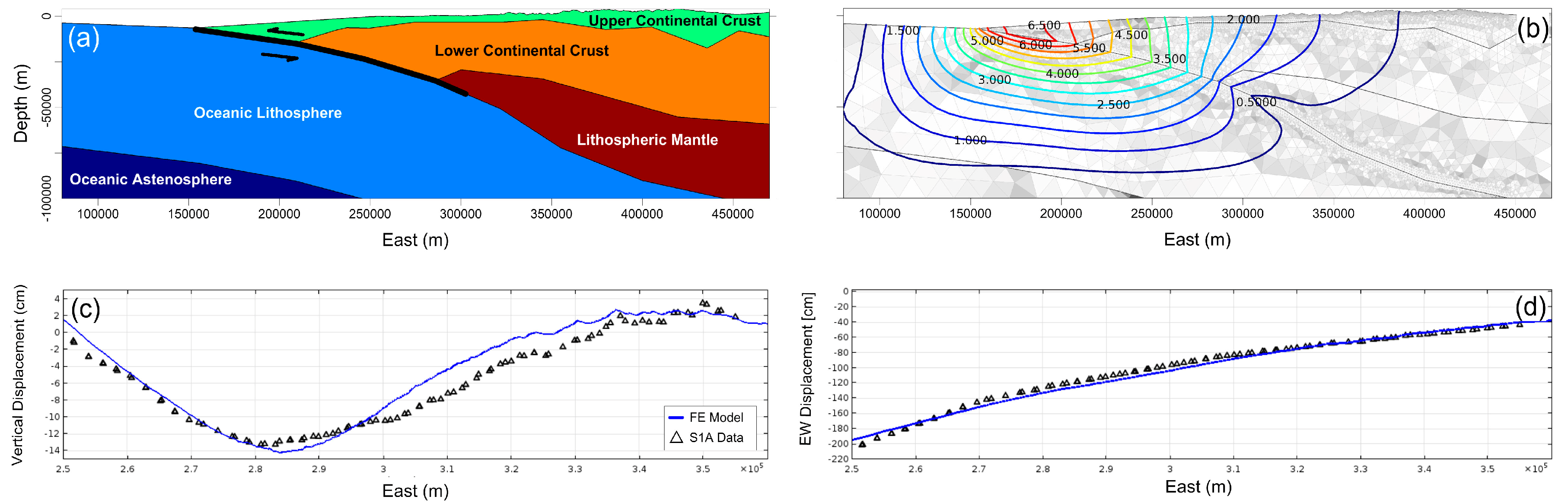
4. Finite Element Modeling

We extend our analysis by performing a 2D numerical modeling of the ground deformation pattern retrieved by the DInSAR measurements; our solution is based on the FE approach and allows us to account for the geological and structural information available over the considered area, as well as the seismicity distribution. More specifically, taking into account the geometric features of the active seismogenic slab and the mechanical heterogeneities, we apply a loading along the shallow segment of the slab (see black line in Figure 5a) in order to simulate the ground deformation pattern. We reproduce the retrieved displacements within a 2D structural mechanical context, under the linear elastic material approximation and by constraining the sub-domain setting with the geological and structural information reported in Tassara and Echaurren [21].

We define a simplified geometry of the study region, which extends 390 km and 100 km deep; such a very large area allows us to neglect the possible edge effects. Concerning the geological setting, we develop a heterogeneous model by considering five geological units having isotropic mechanical properties: (i) upper continental crust; (ii) lower continental crust; (iii) continental mantle; (iv) oceanic lithosphere; and (v) oceanic asthenosphere (Figure 5a). The elastic parameters values are reported in

Table 2. Parameters for each layer defined in the model: Density (kg/m³), Young’s Modulus (GPa) and Poisson Ratio. Modified from [7,21].

Parameters	Upper Crust	Lower Crust	Lithospheric Mantle	Ocean Lithospheric	Ocean Asthenosphere
Density	2700	3100	3300	3300	3400
Young’s Modulus	100	110	150	150	160
Poisson’s Ratio	0.25	0.26	0.26	0.25	0.26

.

As boundary conditions, we apply a free constraint at the upper boundary domain, which corresponds to the topography of the considered area. The bottom boundary is fixed, while a roller condition at the two sides of the numerical domain is applied. The entire numerical domain is discretized in 17,712 tetrahedral elements with a higher refinement along the slab (Figure 5b).

In order to reproduce the coseismic displacement along the fault, we assume the stationarity and linear elasticity of the involved materials by considering the solution of the equilibrium mechanical equations [22]. The earthquake simulation is developed through two stages: During the first one (pre-seismic), the initial stress field was reproduced by applying gravity acceleration under elastic condition; note that this condition permits the model to compact under the weight of the rock successions (gravity loading) until it reached a stable equilibrium [23]. At the second stage, (coseismic), where the stresses are released through a non-uniform slip along the fault, we use an iterative analysis based on a trial-and-error approach [24,25]; it is performed by fixing the location and geometry of the dipping plane constrained by the available structural information and the hypocentral distribution and searching for the loading along the slab. In particular, to evaluate this parameter, we generate several forward structural mechanical models (up to 200) and compare the achieved model results with the EW and vertical component selected along the AA’ profile shown in Figure 3a,b. This profile is selected as it passes through the area of maximum EW displacement.

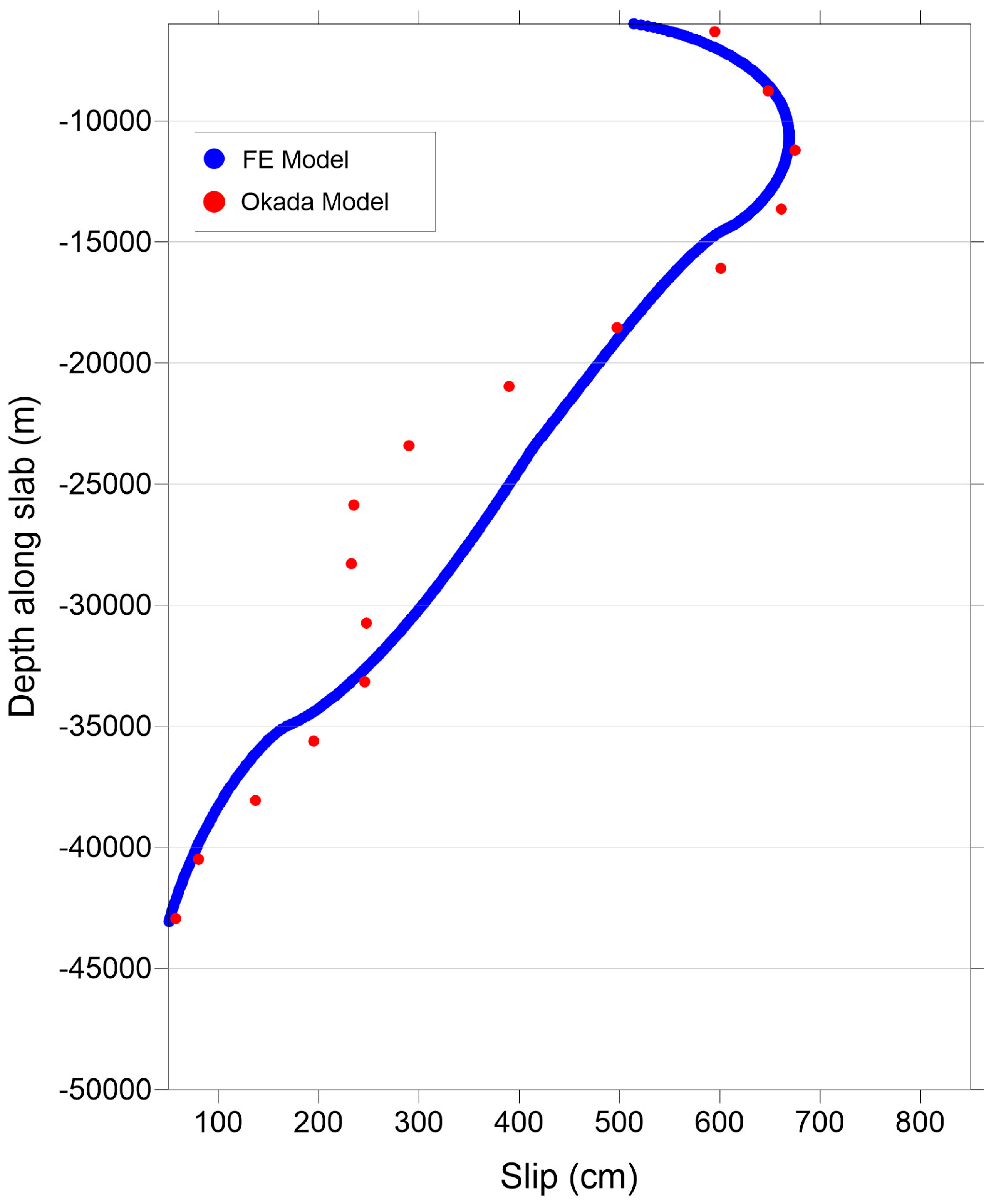
Our best fit model, evaluated by the minimum RMS solution, is reported in Figure 5c,d for the vertical and EW component, respectively. We also report the retrieved 2D displacement along the modeled section, which provides a maximum slip of ~7 m at a depth of 10 km, in the shallower sector of the slab (Figure 5b). A comparison between the slip values retrieved from the FE model and Okada solution along the slab is shown in Figure A3. The achieved major discrepancy, located between depths of 20 and 30 km (hypocentral depth), is probably related to the geometric complexity of subducted slab, considered in the 2D FE model only.

5. Discussion

Our Okada model inferred from the multi-orbit S1A DInSAR measurements shows that almost all of the slip during the 2015 Illapel earthquake occurred northwest of the epicenter at a distance of about 60 km (Figure 4a). A large slip area of about 70 km along strike and 50 km along dip is found with a maximum slip located in the shallowest 20 km. The along-strike extent of the main shock rupture roughly coincides with the trench axis (see green line in Figure 4a). Moreover, the comparison between the slip model map and the aftershock distribution, spanning from 16 September (main shock) to 19 September (corresponding to the last day of temporal coverage of satellite data), reveals that a very small number of aftershocks occurred in the large-slip area (Figure 4a,b); this finding is consistent with what was found by other studies for the Illapel earthquake [6,7,26] and for similar large earthquakes [27]; indeed, the authors of the previous studies, by using the slip distributions for several moderate to large earthquakes, together with their aftershock distributions, concluded that the aftershocks occurred mostly outside or near the edges of the areas of large slip [28]. Our coseismic slip model suggests the slip direction is dominantly downdip and assuming the shear modulus to be 40 GPa, with an average slip of ~4.5 m; the total moment of the preferred model is 2.08 × 10²¹ Nm, corresponding to a moment magnitude 8.1, comparable to the seismic moment magnitude 8.3, calculated by the USGS-National Earthquake Information Center—NEIC [29].

We further improve our analysis by including in the modeling approach the structural and the geological information available for the study area; this allows us to simulate the slip along the subducted slab, stress distribution, and the principal stress axes orientation. To achieve this task, we perform the analysis via a FE approach. Therefore, we make several test in order to search for the loading along the subducted slab; the best model provides a maximum slip of ~7 m at a depth of 10 km, corresponding to the shallower sector of the slab (Figure 5b).

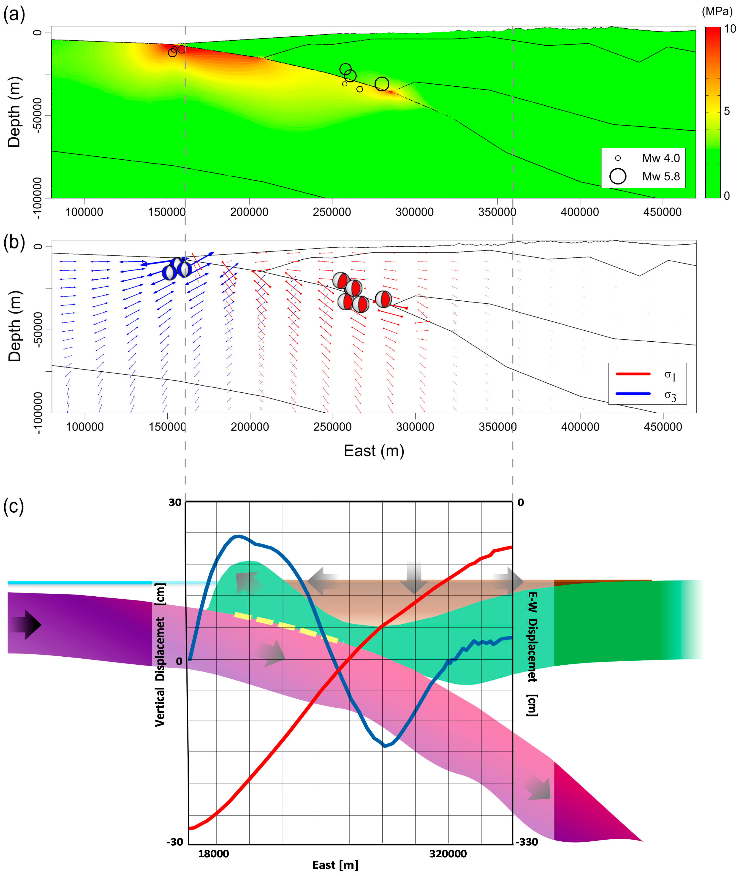
In addition, in order to confirm the validity of our model, we analyze the stress distribution along the subducted slab, in terms of von Mises scalar quantity and orientation of maximum principal stress, and compare them with seismological data. The von Mises stress expresses the difference between the principal components of stress and gives an indication of the amount of shear stress. At the same time, this parameter is proportional to the octahedral shear stress [30] by a constant factor $\sqrt{2}/3$ and thus can be directly compared with the yield strength of the materials to give an estimate of the possibility of failure. Indeed, the obtained von Mises stress distribution, reported in Figure 6a, shows a close similarity with the depth distribution of the aftershock hypocenters. Note that we report one month of aftershocks (with M > 4.3) located within 10 km north and south from the AA’ profile and recorded by GEOFON network. Moreover, the maximum principal stress orientation highlight a compressive regime (horizontally-oriented σ₁) in correspondence of the deeper portion of the slab and an extensional regime (vertically-oriented σ₁) at its shallower segment (Figure 6b). This finding is supported by seismological data that show that at least 3 aftershocks (3 weeks after the main shock) exhibit a high-angle normal faulting close to the trench, and most of the aftershocks share low-angle thrust faulting mechanisms consistent with the megathrust geometry [1] (Figure 6b). Finally, we propose a conceptual model (not to scale) with the aim of synthesizing the kinematics of the megathrust faulting inferred from our modeling results and supported by observed data (Figure 6c). Such a model shows how the megathrust subduction induces a horizontal displacement toward the West, an uplift along the coast and a subsidence behind it of the overriding plate; in the same way, the motion along the subducted slab, considering the distribution of von Mises stress, could explain the occurrence of normal faulting earthquakes (extensional regime) across the trench axis and thrust faulting (compressive regime) along a deeper segment of the slab.

6. Conclusions

Our main findings can be summarized as follows:

• S1A satellite measurements are a powerful tool to analyze the deformation induced by large mega-thrusting earthquakes, as in the case of the Illapel earthquake. More specifically, S1A peculiarities include wide ground coverage (250 km of swath), C-band operational frequency, and short revisit time (that will reduce from 12 to 6 days when the twin system Sentinel-1B will be placed in orbit during 2016). Such characteristics, together with the global coverage acquisition policy, make the Sentinel-1 constellation an extremely suitable region for studying high seismic hazard and monitoring worldwide, thus allowing the generation of both ground displacement information with increasing rapidity and new geological understanding.
• The east–west displacement map highlights a huge westward displacement of about 210 cm, while the vertical displacement map shows an uplifting area of about 25 cm along the coast, surrounded by an annular shaped subsidence of about 20 cm.
• The Okada modeling consists of a reverse fault, accounting for the main seismic event and corresponding to the shallow portion of the subducted slab. Most of the slip occurred northwest of the epicenter at a distance of about 60 km. A large slip area of about 70 km along strike and 50 km along dip is found with a maximum slip located at a depth ranging from 10 to 30 km.
• The FE modeling, obtained by also including our analysis geological and structural information, allows us to estimate values of maximum slip comparable with the analytical solution and to evaluate the von Mises distribution and axis stress orientation, which are in agreement both with the location and the type of faulting of the aftershocks.