Quantifying Multiscale Habitat Structural Complexity: A Cost-Effective Framework for Underwater 3D Modelling

Abstract

Coral reef habitat structural complexity influences key ecological processes, ecosystem biodiversity, and resilience. Measuring structural complexity underwater is not trivial and researchers have been searching for accurate and cost-effective methods that can be applied across spatial extents for over 50 years. This study integrated a set of existing multi-view, image-processing algorithms, to accurately compute metrics of structural complexity (e.g., ratio of surface to planar area) underwater solely from images. This framework resulted in accurate, high-speed 3D habitat reconstructions at scales ranging from small corals to reef-scapes (10s km²). Structural complexity was accurately quantified from both contemporary and historical image datasets across three spatial scales: (i) branching coral colony (Acropora spp.); (ii) reef area (400 m²); and (iii) reef transect (2 km). At small scales, our method delivered models with <1 mm error over 90% of the surface area, while the accuracy at transect scale was 85.3% ± 6% (CI). Advantages are: no need for an a priori requirement for image size or resolution, no invasive techniques, cost-effectiveness, and utilization of existing imagery taken from off-the-shelf cameras (both monocular or stereo). This remote sensing method can be integrated to reef monitoring and improve our knowledge of key aspects of coral reef dynamics, from reef accretion to habitat provisioning and productivity, by measuring and up-scaling estimates of structural complexity.

1. Introduction

Structural complexity is a key habitat feature that influences ecological processes by providing a suite of primary and secondary resources to organisms, such as shelter from predators and availability of food [1,2,3,4]. In terrestrial ecosystems, structural complexity has been related with species diversity and abundance [5,6]. However, while evidence of the importance of the role habitat structural complexity plays in driving key processes in underwater ecosystems exists, the intricacies of the relationships between complexity and important ecological processes are not well understood, due to limitations in the application of current methods to quantify 3D features in underwater environments [7,8]. Thus, our current knowledge of underwater ecosystems and their trajectory is impaired by the lack of understanding of how structural complexity directly and indirectly influences important ecological processes [9]. It is important to incorporate high-resolution and comprehensive measures of structural complexity into assessments that aim to monitor, characterize, and assess marine ecosystems [6].

To date, benthic percent cover, the two-dimensional proportion of coral surface area viewed from above, has been the primary method for monitoring underwater ecosystems [10]. Three-dimensional habitat structural complexity is a key driver of ecosystem diversity, function, and resilience in many ecosystems [11], yet the field of marine ecology lacks the tools to effectively quantify 3D features from underwater environments. Techniques to assess the structural complexity of marine organisms have existed since 1958 [12,13,14]. Currently, the most common method used to quantify habitat structural complexity in marine ecological studies is the “chain-and-tape” method, where the ratio between the linear distance and the contour of the benthos under the chain is calculated as a measure of structural complexity [14,15]. Alternatively, researchers employ a range of techniques to estimate habitat structural complexity, and related metrics, such as surface area and volume [14,16].

On the opposite side of the spectrum, the emergence of satellite remote-sensing techniques has addressed the need for large-scale (10s–1000s m²) and continuous measurements of structural complexity [17,18,19]. Alternatively, swath acoustics can generate digital elevation models with horizontal resolutions of a few square meters [20,21], from which various metrics of habitat complexity, such as slope or surface rugosity (the ration between surface area and planar area), can be quantified across thousands of square meters [22]. Although useful for many applications, these methods are incapable of characterizing underwater structures at high-resolutions (cm-scale) [23,24].

Measuring reef structural complexity, using proxy metrics such as linear rugosity, has greatly contributed to our knowledge of reef functioning (i.e., reef accretion and erosion processes) [3,25,26]. However, advancing our understanding of how structural complexity influences reef dynamics still requires improving our efficiency and ability to quantify multiple metrics of 3D structural complexity in a repeatable way, across spatial extents and maintaining sub-meter resolution [27,28]. Emerging close-range photogrammetric techniques allow the quantification of surface rugosity, among other structural complexity metrics, across a range of spatial extents, and at millimetre to centimetre-level resolution [29,30,31,32,33]. Much of the work in the aforementioned articles builds on a substantial body of work in 3D reconstruction, Optical Flow, and Structure from Motion (SfM) in the terrestrial domain; see [34,35,36,37], among others. Close-range photogrammetry entails 3D reconstructions of a given object or scene from a series of overlapping images, taken from multiple perspectives, enabling precise and accurate quantification of structural complexity metrics [38]. Underwater cameras provide a useful solution, and by capturing high-resolution imagery of the benthos, they rapidly obtain a permanent record of habitat condition over ecologically relevant spatial scales [39].

Unsurprisingly, the use of cameras to measure structural complexity is a rapidly evolving field [40]. Initially, multiple cameras were used to gather high-quality image data and generate 3D reconstructions of underwater scenes, from which multiple metrics of habitat complexity can be quantified [38,41]. Stereo-imagery workflows tend to be better streamlined than monocular ones, but there is a significant cost associated with the purchase and operation of such equipment [39,40]. While stereo-cameras enable data collection at the desired resolution and spatial scales, they preclude the quantification of structural complexity to the periods preceding their development, limiting their use to contemporary and future studies [39,42]. As most existing video/photo surveys to date have used monocular cameras, it is clear that there is a great need for a method to produce accurate 3D representations of underwater habitats using data collected by off-the-shelf, monocular cameras [18,19,42]. Such methods would enable the analysis and use of historical data, providing a unique opportunity to understand the role of structural complexity in underwater ecosystems and their temporal trajectory. Thus, this study focuses on monocular-derived photogrammetry from an uncalibrated camera, and does not refer to studies involving multiple cameras or other instruments to build 3D reconstructions of underwater scenes.

In relation to coral reef ecosystems, close-range photogrammetry was first used by Bythell et al. in 2001 [43] to obtain structural complexity metrics from coral colonies of simple morphologies. The popularity of photogrammetry has increased as the algorithms behind it improved and a few studies have evaluated the accuracy of its application to underwater organisms, from simple morphologies [16] to more complex ones [29,31,44,45]. Yet, it took over a decade to enable the application of photogrammetry to medium and large underwater scenes using, exclusively, images captured using monocular off-the-shelf cameras [32,33].

In this study, we developed a suite of integrated algorithms that incorporate existing methods for measuring structural complexity underwater to allow their application to monocular data obtained from off-the-shelf underwater cameras. While this is not the first time that Structure from Motion (SfM) has been applied underwater [16,31,32,33,43], this framework integrates existing methods in an unprecedented way. Our approach involves a set of multi-view, image-processing algorithms, which provide rapid and accurate 3D reconstruction from images captured with a monocular video or still camera. It is an innovative method for accurately quantifying structural complexity (and related metrics) of underwater habitats across multiple spatial extents at cm-resolution. This framework satisfies the following criteria, which define the need for measuring structural complexity from historical data captured using only off-the-shelf cameras in various underwater habitats. There are existing methods that accomplish one or more of the outlined requirements [31,32,33]; however, this is the first study to present evidence and demonstrate how this approach satisfies all of the requirements over multiple spatial scales. Thus, successfully demonstrating how historical data (i.e., benthic video transects) can be used to build 3D terrain reconstructions and its suitability for coral reef monitoring (i.e., cost effective):

(i)

It works for images recorded in moderately turbid waters with non-uniform lighting.

(ii)

It does not assume scene rigidity; moving features are automatically detected and extracted from the scene. If the moving object appears in more than a few frames, the reconstructed scene will contain occluded regions.

(iii)

It allows large datasets and the investigation of structural complexity at multiple extents and resolutions (mm² to km²).

(iv)

It allows in situ data acquisition in a non-intrusive way, including historical datasets.

(v)

It enables deployment from multiple imaging-platforms.

(vi)

It can obtain measurement accuracies <1 mm, given that at least one landmark of known size is present to extract scale information. Note that as the reconstruction is performed over a larger area its resolution will decrease.

Here, we describe this framework and demonstrate its ability to accurately measure structural complexity across three spatial extents, using coral reefs as an example. Note that while we provide examples of three extents here, it is possible to calculate structural complexity estimates across multiple extents and resolutions from these 3D models. We use data collected exclusively from monocular video/photo sequences to generate highly accurate 3D models of a single coral colony, a medium reef area and 2 km long reef transect, from which measurements of structural complexity (surface rugosity, volume rugosity, volume, and surface area) are obtained.

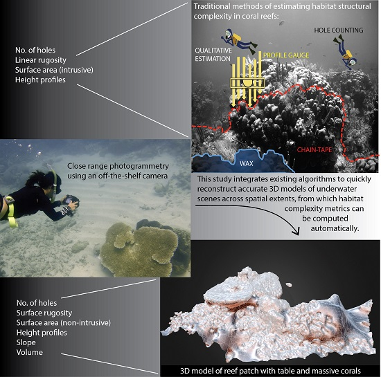
2. Materials and Methods

We combined existing algorithms to generate a 3D dense topographic reconstruction of underwater areas at three spatial extents: (1) a branching coral colony taking multiple monocular still images; (2) a 400 m² reef area imaged with monocular video sequences by a diver; and (3) 2 km long (4–30 m wide) reef transects imaged with video sequences by a diver using an underwater propulsion vehicle (see Gonzalez-Rivero et al. 2014 [46] for details). Regardless of the extent the same procedure is applied (Figure 1). There is no intrinsic method for computing the absolute scale within the scene from monocular data; this was resolved by using known landmarks, which were measured in situ. Reference markers were not used because we wanted to assess the suitability of this framework to historical data sets, where reference markers or ground control points (GCP) are not normally present, but where manually-measured in situ landmarks are common. The following sections describe each step of the processing method and provide the details of the algorithms involved, which apply to all scales unless otherwise specified.

Figure 1. Processing modules and data flow for underwater 3D model reconstruction and validation process.

Figure 1. Processing modules and data flow for underwater 3D model reconstruction and validation process.

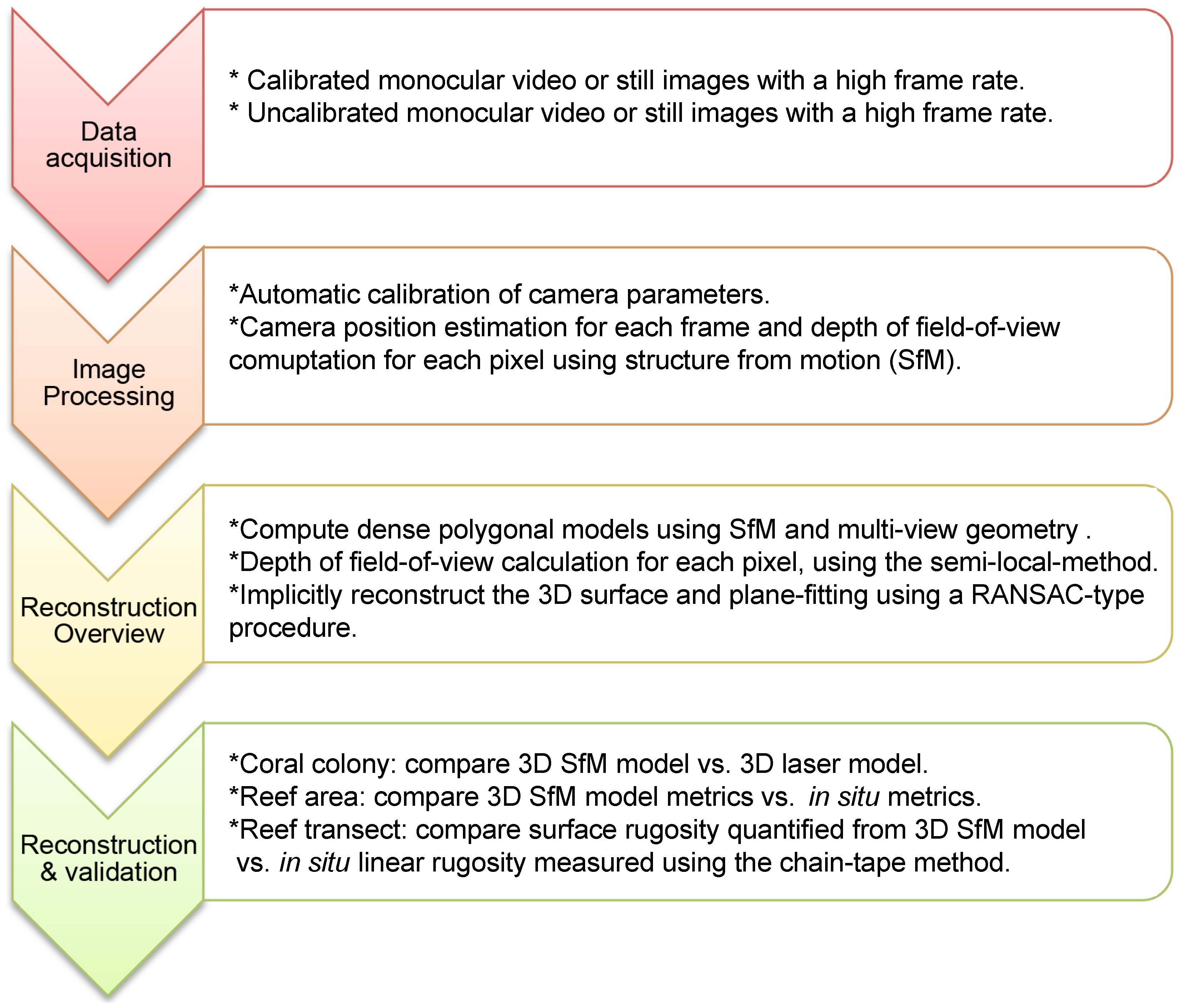
2.1. Data Acquisition

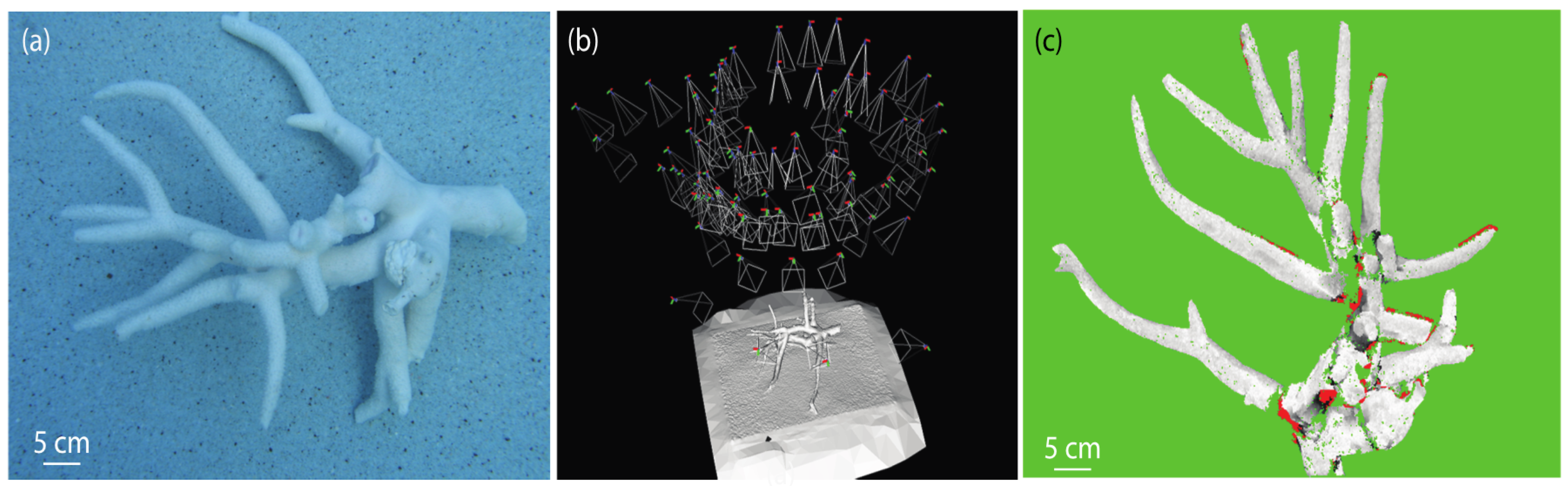
2.1.1. Calibrated Data: Coral Colony

A total of 84 underwater still images of a branching Acropora spp. coral were captured in a swimming pool using a Canon PowerShot G2 camera enclosed in a custom IkeLite housing, with a resolution of 2272 × 1704 pixels, and images were captured at an altitude of 1–1.5 m. At this resolution, a pixel spans roughly 174 μm of the surface of the coral (the colony was ~35 × 25 × 15 cm in size). Calibration of key parameters, such as focal length is not required for this framework as they are computed concurrently with the 3D reconstruction. The camera was initially calibrated by imaging a standard planar calibration grid, with 70 × 70 mm squares, underwater from 21 viewpoints over a hemisphere with an approximate altitude of 0.8 m (Figure 2). A modified version of the Matlab Calibration Toolbox [47] was used to compute the intrinsic and distortion parameters automatically [48] for details see [29] and SM5.

Figure 2. (a) Sample image collected for use in the reconstruction of the branching coral; (b) camera positions used to compute the 3D reconstruction of the coral; and (c) gathered error statistics for the coral with variance σ = 0.1 mm. Green denotes no ground-truth measure due to occlusion, red a gross error (>10σ), white no error increasing towards black (10σ).

Figure 2. (a) Sample image collected for use in the reconstruction of the branching coral; (b) camera positions used to compute the 3D reconstruction of the coral; and (c) gathered error statistics for the coral with variance σ = 0.1 mm. Green denotes no ground-truth measure due to occlusion, red a gross error (>10σ), white no error increasing towards black (10σ).

2.1.2. Uncalibrated Data: Reef Area and Reef Transect

An area on the forereef of Glovers Reef (87°48′ W, 16°50′ N), located 52 km offshore of Belize in Central America, was filmed and mapped by divers during 2009. The perimeter of approximately 400 m² of forereef was marked using a thin rope (5 mm in diameter), and subdivided into 4 m² quadrats by marking the corners of each quadrat. The reef area was filmed using a high-definition Sanyo Xacti HD1010 video camera (1280 × 720 at 30 Hz and 30 frames per second, field of view 38–380 mm range) in an Epoque housing held at an altitude ranging between 1 and 2 m following the contour of the reef (depth of 10–12 m).

Quadrats were imaged consecutively in video-transects (20 m × 2 m each) following a lawnmower-pattern, with at least 20% overlap between each consecutive transect. This process was repeated to reconstruct the entire reef area of 400 m². Multiple overlapping images were obtained from the video data. The SfM algorithm computed the location of the camera relative to the reconstructed scene by assuming that the corals being imaged were not moving. Hence, the location of the camera relative to the scene did not affect the reconstruction [49,50].

Kilometer-length transects were collected using a customised diver propulsion vehicle (SVII) where two Go-Pro Hero 2 cameras in a stereo-housing (Go-Pro Housing modified by Eye-of-mine with a flat view port) are attached facing downwards (see [46] for details). Video data in high-definition, at a rate of 25 frames per second, were captured at a constant speed of 1 knot and at 1.5–2 m altitude from the substrate, following the 10 m depth contour line of the reef. To alleviate the curve distortion introduced by the focal properties of the wide-angle lenses, the cameras were configured to “narrow” Field of View (FOV), which brings the FOV from 170 to 90 degrees. Using these settings, the intrinsic and extrinsic parameters of the camera configuration were obtained using a customized calibration toolbox in MatLab [48]. Finally, the 3D reconstruction applied the corresponding calibration parameters. It is important to point out that the calibration was only used for setting the camera configuration, rather than for calibrating the actual reconstruction of every dataset.

Using this framework, 2 km-linear transects have been captured per dive (45 min) in major bioregions around the world: Eastern Atlantic, Great Barrier Reef, Coral Sea, Coral Triangle, Indian, and Pacific Oceans [46]. Cameras are synchronized in time with a tethered GPS unit on a diver float, which allow geo-referencing the images collected as the SVII move along the reef [46].

2.2. Image Processing

The initial automatic calibration procedure consisted of feature extraction and tracking over a short video-sequence, followed by simultaneous camera positioning and intrinsic parameter estimation. The intrinsic parameters obtained in the first phase were used to compute camera poses and dense 3D point clouds of the entire scene [51]. Finally, an implicit surface reconstruction algorithm was used to fuse the 3D points.

2.3. Reconstruction Overview

2.3.1. Structure-from-Motion (SfM)

To compute camera poses and 3D sparse points we modified the SfM system from [52] for application to monocular cameras. This first step calculated a set of accurate camera poses associated to each video frame along with sparse 3D points representing the observed scene.

2.3.2. Depth of Field-of-View

The second step established (on a per-frame-basis) the depth of field-of-view of the scene associated with all the pixels in each frame [53,54,55]. Once the depth of a pixel location was determined, we back-projected a pixel into the scene as a 3D point on the surface of an object [51]. This algorithm generates highly accurate sets of dense 3D points for each frame, e.g., >80% of pixels have less than 30 mm error for ranges >5 m; for details see [29]. This framework estimated depth of field-of-view with an iterative algorithm called the Semi-Local Method (Algorithms 1 and 2 in [51] ) where) (i) a plane sweep finds an initial depth estimate for each pixel [56]; (ii) depth is refined by assuming that depths for neighboring pixels should be similar [57]; and (iii) depths are checked for consistency across neighboring images.

2.3.3. Implicit Surface Reconstruction

Parametric 3D reconstruction methods have been proven problematic to maintain the correct topography of 3D models [58,59]. Thus, step three employed an implicit 3D reconstruction method to ensure accuracy of the resultant reconstruction, which fused 3D data (depth estimates) into a volume of finite size that encapsulates the total extent of the object/scene [53,54,55,60]. Then, we processed the volume and approximated a solution for the surface that best fits the observed data. To achieve this, this framework computed a set of oriented 3D points to be inputted into the implicit surface reconstruction. Then, we performed a RANSAC-type [61] plane-fitting procedure on the depth estimates, resulting in a set of oriented 3D points for each image. The point set was then fused into a 3D polygonal model using a Poisson reconstruction method [62]. This 3D polygonal model is the final representation from which we compute relevant structural complexity metrics.

2.4. Model Reconstruction and Validation

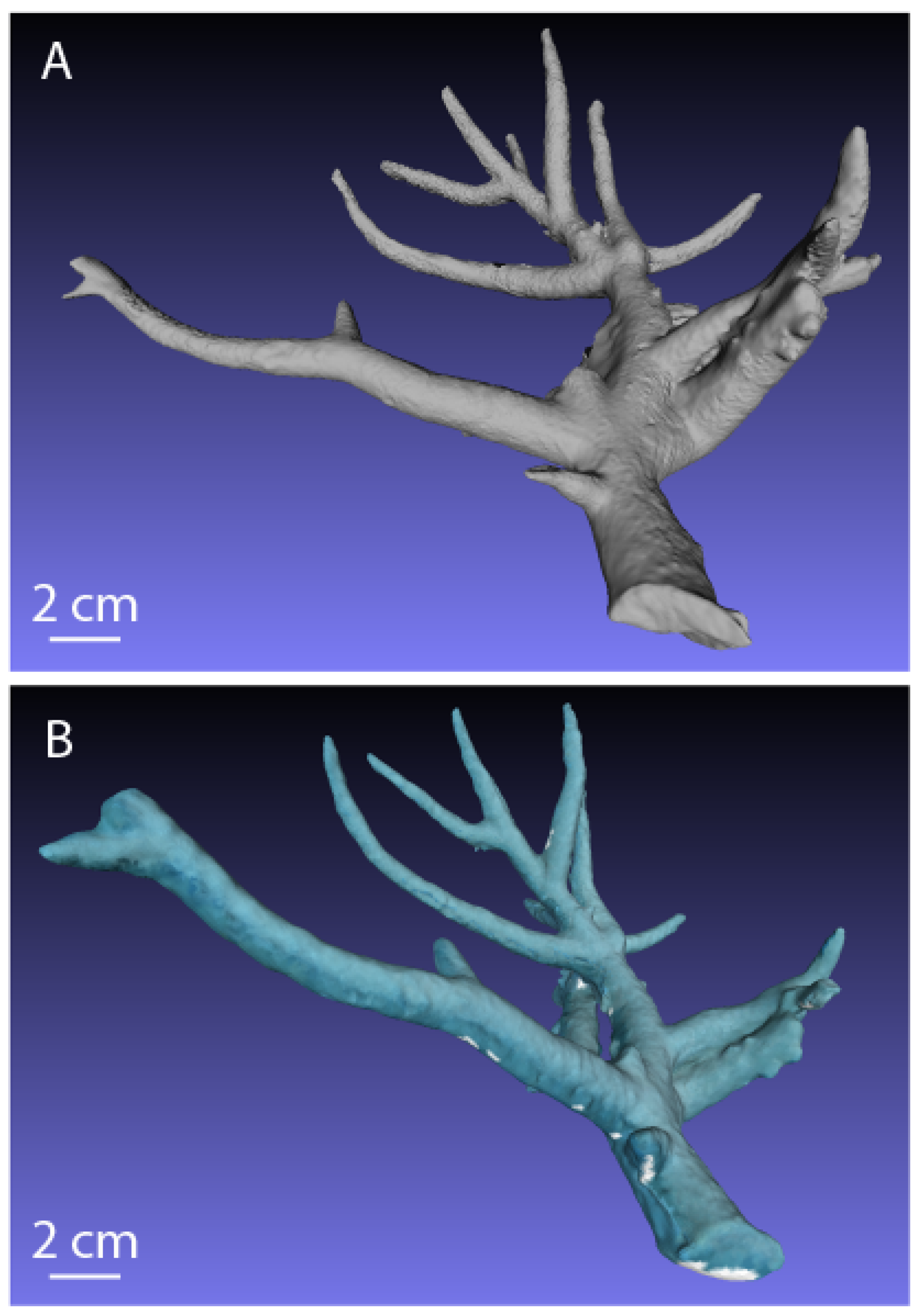
2.4.1. Branching Coral Colony 3D Model

To obtain an accurate reference 3D model of the coral for validation, we imaged the coral skeleton multiple times with a Cyberware Model 3030/sRGB laser-stripe scanner outside of the water. The resolution of each scan was 350 μm. The laser scanner rotates completely around the object in a continuous hemispheric trajectory to provide a 3D model. Due to occlusions, a total of two scans were acquired with the coral in different poses for each of the scans. Each 3D laser model was aligned using Iterative Closest Point [63], and then merged together to form the single reference model (Figure 3A). Merging the multiple scans increases the effective resolution due to the increased density of point measurements.

To obtain the test 3D model of the coral a total of 84 images were acquired underwater, low quality (e.g., blurry) images were removed resulting in 60 images that were used to compute the reconstruction (Figure 2a,b). The piece of coral was flipped over halfway through the data collection process to minimize occlusions and make the underwater 3D model more comparable to the validation 3D model, thus our accuracy applies to the entire surface area of the coral. In situ, it may prove difficult to image a coral colony from all angles, however the quoted accuracy still applies to all surfaces seen in the collected data. The inability to rotate the coral will potentially result in occlusions, but will not affect the accuracy of the proposed method. The test and the reference models were subsequently aligned using Iterative Closest Point [50] to evaluate the accuracy of the underwater 3D reconstruction. The alignment parameters consisted of a rotation, translation, and uniform scale. In other words, the alignment process enabled by the integrated algorithm framework is able to detect common features and correlate them with other views of the same area. The entire contribution of this work is the possibility to take images from multiple views and align or fuse them together to create accurate and dense 3D reconstructions.

Figure 3. (A) Laser-scan reference model of the branching coral acquired with a Cyberware laser-stripe scanner; and (B) final 3D reconstruction of the coral.

Figure 3. (A) Laser-scan reference model of the branching coral acquired with a Cyberware laser-stripe scanner; and (B) final 3D reconstruction of the coral.

2.4.2. Reef Area and Reef Transect 3D Model

Reef Area Validation Data

Divers mapped and characterized the benthos of the reef area. For each quadrat all structures with a diameter ≥ 10 cm were mapped and measured to the nearest centimeter. Three measurements were taken from each structure: (1) maximum diameter (x); (2) perpendicular diameter (y; both axes perpendicular to the growth axis); and (3) maximum height (z; parallel to the growth axis).

Corals were assumed to have an elliptical cylinder shape, and simple geometric forms were assumed to estimate the surface area and volume of each colony from morphometric parameters measured in situ (z, x, and y). Equation (1) was used to calculate the structural complexity of each quadrat (SC_quadrat), as a proportion of the total volume of all structures in a quadrat and the total volume of that quadrat, assuming the same maximum height across all quadrats.

$$S{C}_{quadrat}=\frac{\sum \pi ab{h}_{colony}}{4l_{quadrat }{w}_{quadrat }{h}_{quadrat}}$$

(1)

where a is the radius of the maximum diameter of an ellipse representing the top of a coral colony (x/2) and b is the radius of the perpendicular diameter to the maximum diameter of the same ellipse (y/2); h_colony is the maximum height (z) of the same colony; l_quadrat and w_quadrat denote the length and width of each quadrat, respectively, and h_transect denotes the maximum height of all quadrats. A highly-complex quadrat would have a value close to 1, while a quadrat with very low complexity would have a value close to zero. The volume and surface area were calculated for each quadrat by combining the spatial distribution and size data using the equations in SM1.

Reef Area Underwater 3D Model Reconstruction

As the camera parameters (focal length, principle points, distortion, etc.) were unknown for this dataset, calibration results were determined during processing using known landmarks in the scene. The reconstruction of each transect may be rendered at different relative scales because our framework is based on monocular data. Thus, each transect was individually reconstructed and scaled to the same global scale using in situ measurements.

To validate the underwater 3D model of the reef area we measured x, y, and z of each feature in the 3D model and applied Equation (1) to calculate structural complexity. The initial reconstructions did not lie in the same coordinate system as in situ measurements; thus, metric dimensions were used to align reconstructions to the same coordinate system. A robust plane-fitting algorithm was applied to determine the normal direction of sea floor in a traditional coordinate system in the Euclidean space. This framework excluded moving objects (fish, gorgonians, etc.) from the final reconstruction when an object was not seen in at least three frames (number is user specified), based on the iterative process presented in McKinnon Smith and Upcroft [51]. Sometimes this process generates sparsely-rendered regions in the reconstruction; gathering additional video data in regions with significant moving features would resolve this issue.

The maximum height for each quadrat was computed by Equation (2):

$$h_{max}\left(i\right)=\{\begin{array}{c}{h}_{max}^1\left(i\right), h_{max}^1\left(i\right)>h_{max}^2\left(i\right)\\ h_{max}^2\left(i\right), h_{max}^1\left(i\right)<h_{max}^2\left(i\right)\end{array}$$

(2)

where, h_max(i) is the maximum height in the i-th quadrat, h¹_max(i) and h²_max(i) denote the maximum height for the i-th quadrat on the left half-transect and the right half-transect, respectively. The structural complexity of the first transect is defined as the volume integral over each quadrat as in Equation (3):

$$S{C}_{quadrat}\left(i\right)={\int }^{}{h}_i\left(x,y\right) dx dy$$

(3)

where i is the index of the quadrats in the first transect, h_i(x, y) is the height distribution of each quadrat. While dx and dy denote the size of the grid by which each quadrat is approximated.

Reef Area Underwater 3D Model Validation

We used two metrics to validate the underwater 3D model of the reef area: (1) maximum height (measured in situ); and (2) structural complexity. We directly compared height measured in situ with height measured from the virtual underwater 3D model. Similarly, we used a two-tailed pairwise t-test, to compare the structural complexity calculated from the morphometric parameters measured in situ against the structural complexity calculated from morphometric parameters measured in the underwater 3D model. The accuracy of the underwater 3D model was evaluated by the relative absolute error (RAE) as in equation (4) [64]. The RAE calculates a proportion of the difference between measurements; e.g., zero reflects that the values are exactly the same, while 0.5 reflects a 50% difference between values. In this study, we arbitrarily chose 25% as a threshold to determine a large error.

$$RAE=\frac{|X_E-X_{G }|}{X_G}$$

(4)

where X_E is the structural complexity calculated from the underwater 3D model, and X_G from the in situ measurements. Finally, we compared the structural complexity calculated from the morphometric parameters measured in situ against the structural complexity calculated directly from the underwater 3D model.

Reef Transect Underwater 3D Model Reconstruction

The frames from video collected along the 2 km-transects were extracted and divided into 200-frame sections to reconstruct 3D models for every 10 m reef transect sections, approximately, along the transect. This procedure allow for accounting cumulative projective drift and hence model distortion [65] by resetting the reconstruction parameters every 200 frames. While two cameras were used in stereo for capturing video data, here the reconstruction of the 3D model was done using the left camera and only using one frame of the right camera, per every 10 m section, to aid scaling the model. Camera parameters (focal length, principle points, distortion, etc.) were calibrated using track-from-motion algorithms of a reference card (sensu [64]). Parameters were optimized to a single set for all reconstructions. Using these parameters, the protocol described above is applied to each subset of frames to produce 3D model reconstructions along the entire 2 km transect.

Reef Transect Underwater 3D Model Validation

Structural complexity, from transect models, was calculated as the surface rugosity index (SR), defined by the ratio of convoluted surface area of a terrain (A), and the area of its orthogonal projection of a 2D plane (Ap) Equation (5), for every tracked point in the point-cloud generated by the reconstruction (sensu [38]). Each point on the model (xy) served as a centroid of a 4-m² quadrat, delineating portion of the model where surface rugosity was calculated. This way, surface rugosity was estimated as a continuum along each transect:

$${\text{SR}}_{\text{xy}}=\frac{\mathrm{A}}{{\mathrm{A}}_{\mathrm{p}}}$$

(5)

For the purpose of validation, linear rugosity was also estimated in the field using the chain-tape method [15,25], where a chain (10 m length and 1 cm link-size) was laid over the reef, following the reef contour in a line. Linear rugosity was then calculated as the ratio of the length of chain in a straight line (10 m) by the linear length of chain when following the reef contour. The estimation of surface rugosity from the 3D models, described above, follows the same principle, but considering two dimensions, rather than a linear assessment.

Linear and surface rugosity are highly correlated [38], thus we use linear rugosity to validate the 3D model surface rugosity estimations. Therefore, using the method described above, video data was captured over 17 sections where the chain was laid, and the accuracy of the model-derived surface rugosity (Acc) was estimated as one minus the relative absolute difference between the chain-tape (Rc) linear rugosity and the median values of model-derived ($\overline{{\mathrm{R}}_{\mathrm{m}}}$) surface rugosity Equation (6). Accuracy is here presented as a percentage; therefore 100 multiplied by the relative accuracy. Values approximating zero indicate high dissimilarity between the surface rugosity and linear rugosity values; while values close to 100 indicate high accuracy. However, it is necessary to state that, while the chain-tape method is a standard approach in ecology to estimate coral reef rugosity, it is one of a variety of metrics to assess structural complexity, not the accuracy of the 3D reconstruction directly:

$$Acc=\left(1- \frac{\left|R_c-\overline{R_m}\right|}{R_c}\right)·100\%$$

(6)

3. Results

3.1. Branching Coral: Laser-Scanned Model vs. Underwater 3D Model

The accuracy of the 3D reconstruction generated by this framework was <1 mm over 90% of the surface of the coral, with the largest error being 1.4 mm, further details in [29]. Images were captured under the water using a CCD camera with a resolution of 2272 × 1704 pixels at a distance of 1 m–1.5 m. At this resolution, the Ground Sample Distance (GSD), or size of a pixel in the image, is approximately 3.144 μm per pixel on the surface of the coral which is approximately 35 mm × 25 mm × 15 mm in size. The average alignment error between vertices of the two models was 0.7 mm, indicating a high accuracy of the underwater 3D reconstruction. We were able to flip this piece of coral over to obtain images of all surfaces; thus, our accuracy applies to the entire surface area of the coral. The error of the depth estimates over the entire image is illustrated with a cumulative distribution function (CDF) as a percentage of total pixels (Figure 4). Seventy-seven percent (77%) of the pixels in the reconstruction had a depth within 0.3 mm of the ground-truth depth (Figure 4, SM2 video of the underwater 3D model of branching coral).

Figure 4. Cumulative Distribution Function (CDF) for depth estimates, given as a percentage of the total pixels in the reconstruction. The CDF gives the percentage of total pixels in the image with a variance less than or equal to a given value of σ. Here σ = 0.1 mm and 77% of the pixels in the reconstruction have a depth that is within 3σ = 0.3 mm of the ground-truth depth.

Figure 4. Cumulative Distribution Function (CDF) for depth estimates, given as a percentage of the total pixels in the reconstruction. The CDF gives the percentage of total pixels in the image with a variance less than or equal to a given value of σ. Here σ = 0.1 mm and 77% of the pixels in the reconstruction have a depth that is within 3σ = 0.3 mm of the ground-truth depth.

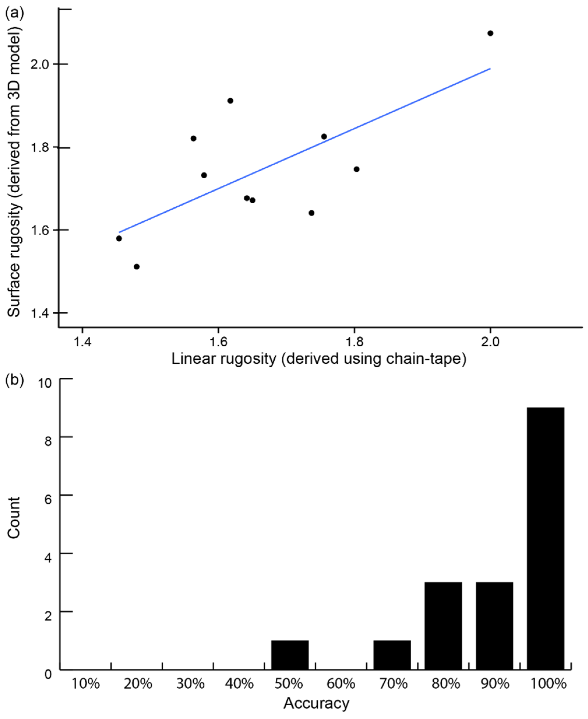
3.2. Reef Area: In Situ Metrics vs. Underwater 3D Model Metrics

The reef area was imaged using a high-resolution (1280 × 720) Sanyo Xacti HD video camera at a 1 m–2 m altitude to the planar reef area. The sensor size and focal length of our deployed camera are 5.76 mm × 4.29 mm and 6.3 mm, respectively. Thus, each image has an approximate footprint of 1.8 m × 1 m, and the corresponding GSD is approximately 0.14 cm per pixel over the surface of the reef area. Note that the sea floor is not even, which indicates peak areas have even smaller GSD, while valley areas have larger GSD. The average error and confidence interval (95%) in reef height across all quadrats was 17.23 ± 13.79 cm (Figure 5a), and the maximum error in any given quadrat was 31.02 cm. The average (±SE) accuracy for colony height across all quadrats was 79% ± 3% (Figure 5a). Differences in maximum height where larger than 25% in quadrats 3 and 10. If these quadrats are removed from the analysis, the average error and confidence interval for the remaining quadrats is 15.69 ± 8.2 cm (Figure 5a), with a maximum error of 23.89 cm. The accuracy when excluding these quadrats is 82% ± 2%. The analysis was run twice, once with and once without the quadrats, to demonstrate the robustness of our framework to errors.

The structural complexity calculated from the morphometric parameters measured in situ did not differ significantly to the structural complexity calculated from morphometric parameters measured in the underwater 3D model (Figure 5b, p-value 0.359, SD = 0.1). Quadrat 1 was only partially reconstructed due to human error during data acquisition (the camera only started recording half-way through the quadrat), resulting in a difference between the in situ and the 3D estimations of structural complexity for that quadrat (Figure 5b). Consequently, we compared the 3D model estimates with the in situ data twice, once including all quadrats, and once excluding quadrat 1. Excluding quadrat 1 did not make a significant difference (p = 0.937, SD = 0.02); thus, this framework is robust to error.

Assuming geometric shapes underestimated the structural complexity by almost 50% (Figure 5b), probably because assuming geometric forms potentially introduces a large error when an object’s cross-section is not an ellipse. Our framework empirically computed the exact measurements from the 3D model, by not assuming geometric forms, this framework yielded values much closer to the true structural complexity of the reef (Figure 6, SM3 video of the 3D model of reef area).

Figure 5. (a) Comparison between the maximum height for quadrats 1–10: in situ measurements (black), estimations from 3D reconstructed model (grey); and (b) comparison between the structural complexity for quadrats 1–10: in situ measurements (black), 3D reconstructed model, which assumes simple geometric forms (grey) and the underwater 3D reconstructed model, which takes into account the actual shape (light grey). Structural complexity was calculated as in Equation (1), where a value of 1 represents a highly complex quadrat and a value of 0 a flat quadrat.

Figure 5. (a) Comparison between the maximum height for quadrats 1–10: in situ measurements (black), estimations from 3D reconstructed model (grey); and (b) comparison between the structural complexity for quadrats 1–10: in situ measurements (black), 3D reconstructed model, which assumes simple geometric forms (grey) and the underwater 3D reconstructed model, which takes into account the actual shape (light grey). Structural complexity was calculated as in Equation (1), where a value of 1 represents a highly complex quadrat and a value of 0 a flat quadrat.

Figure 6. Heat-map of structural complexity of a section of a 400 m² reef area. Both x and y axes are marked in meters, each quadrat is 2 × 2 m. Structural complexity was calculated as in Equation (1), where a value of 1 represents a flat quadrat, and a higher value a more complex quadrat.

Figure 6. Heat-map of structural complexity of a section of a 400 m² reef area. Both x and y axes are marked in meters, each quadrat is 2 × 2 m. Structural complexity was calculated as in Equation (1), where a value of 1 represents a flat quadrat, and a higher value a more complex quadrat.

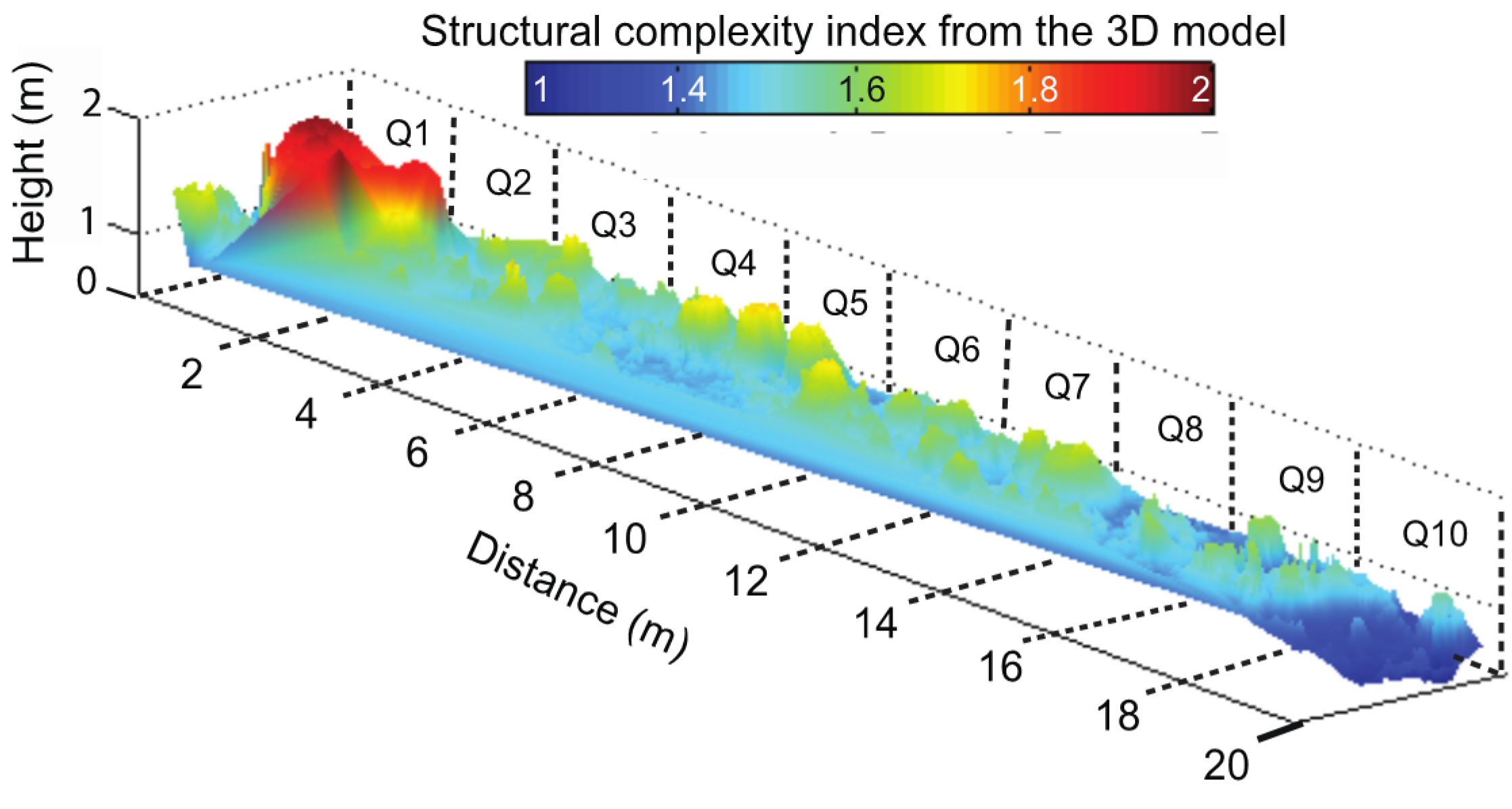
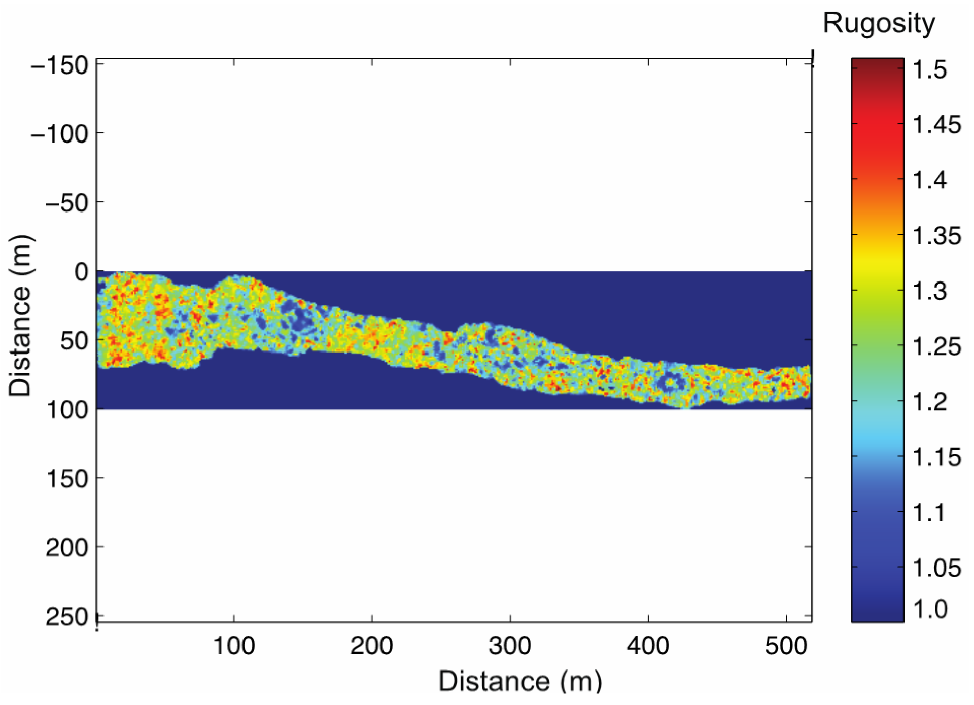
3.3. Reef Transect: In Situ Metrics vs. Underwater 3D Model Metrics

With and altitude between 2 and 3 m the GSD for the Go-Pro imagery ranged between 0.02 and 0.03 cm per pixel. Similar to the reef area, GSD applies to planar images, so peaks would have a higher GSD while valleys would have a lower one. Having a reference object would increase the accuracy of the GSD estimation for a particular region along the reconstructed 3D transect. Using surface rugosity as a proxy measurement of structural complexity, we measured both surface rugosity and linear rugosity in 17 transect-sections (Figure 7). Comparisons between linear rugosity, measured in situ by the chain-tape method, vs. surface rugosity, measured from the reef transect 3D model, resulted in a geometric mean of 85.3% ± 6.0% (±95% CI, Figure 8). These results suggest the used framework is highly accurate at small spatial extents and accurate at both medium and reefscape extents (SM4 video of the 3D model of reef transect-section).

Figure 7. Heat-map of surface rugosity of a section of a 500 m of the reef transect. Both x and y-axes denote distance in metres, the transect width ranged from 4 to 30 m. Surface rugosity was calculated in 2 × 2 m quadrats. Structural complexity was calculated as in [30], where a value of 1 represents a flat quadrat and the index increases with habitat structural complexity.

Figure 7. Heat-map of surface rugosity of a section of a 500 m of the reef transect. Both x and y-axes denote distance in metres, the transect width ranged from 4 to 30 m. Surface rugosity was calculated in 2 × 2 m quadrats. Structural complexity was calculated as in [30], where a value of 1 represents a flat quadrat and the index increases with habitat structural complexity.

Figure 8. Accuracy of surface rugosity estimations from 3D reconstructions of transects when compared against linear rugosity measured in the field by the chain-tape method. Panel (a) is the correlation between surface and linear rugosity, while panel (b) shows the histogram of values recorded for 17 observations, where overall accuracy detected for this method was 85.3% ± 6.0% (geometric mean ± 95% Confidence Interval).

Figure 8. Accuracy of surface rugosity estimations from 3D reconstructions of transects when compared against linear rugosity measured in the field by the chain-tape method. Panel (a) is the correlation between surface and linear rugosity, while panel (b) shows the histogram of values recorded for 17 observations, where overall accuracy detected for this method was 85.3% ± 6.0% (geometric mean ± 95% Confidence Interval).

4. Discussion

This study combined existing methodologies for generating accurate 3D models of underwater scenes at multiple spatial extents using data gathered with off-the-shelf monocular cameras. We present three examples where this framework was used to quantify surface area, height profiles, volume and surface rugosity of coral reefs, across three different spatial extents and with high-resolution. Additionally, the validation analyses showed accuracies ranging from 79% (reefscape) to 90% (coral colony), in agreement with previous studies assessing accuracies for photogrammetric measures of coral colonies [28,31,43,66,67,68]. These results show evidence of the utility of this framework to coral reef ecology and monitoring, in particular given the rapid degradation of coral reefs worldwide, for example they could enable the monitoring of coral reef flattening after a bleaching event [69]. While recent photogrammetric studies have shown similar accuracies, worthy of highlighting is the capacity of this framework to quantify 3D metrics of habitat structural complexity from historical data, captured by off-the-shelf monocular cameras without reference objects present in the scene. In the following sections we discuss the accuracy and efficiency of the framework here presented, its advantages and limitations, its applications to measure and monitor reef structural complexity, and provide specific examples of how this framework can bridge existing knowledge gaps in understanding drivers behind reef biodiversity, function, and resilience of coral reefs.

4.1. Methodological Accuracy and Validation

Accuracy estimates from models ranged from 79% to 90%, according to the spatial extent (from colony to reefscape). It is important to highlight that reference markers were not used because we wanted to assess the suitability of this framework to historical data sets (where reference markers or GCP are not normally present); thus, accuracy of the models were measured using different reference metrics for each spatial extent and, therefore, the interpretation of accuracy varies for each extent. 3D reconstructions of coral colonies could be contrasted against the most accurately available data, laser reconstruction, which has sub-millimetre precision and accuracy [51]. This confirms that 3D reconstructions from monocular cameras can recreate the three-dimensional complexity of coral reef colonies with a very high resemblance to laser scanners and with enough precision to monitor key processes, such as coral growth and erosion.

Given the challenges of underwater imaging (i.e., light attenuation and scattering), the increase of morphological complexity at the reef level and the trade-off between coverage and imaging effort, our next question was, could 3D reconstructions obtained applying this framework at large spatial extents quantify habitat structural complexity? If so to what level of accuracy? The challenge for measuring the accuracy of 3D models at the reef level was finding reference metrics that accurately captured structural complexity. In the absence of having access to an alternative and method proved highly accurate to recreate the three-dimensional structure of the reef, here we decided to use traditional metrics as proxy values for reef complexity (e.g., rugosity, substrate height). Although highly useful to understanding ecological processes and patterns [11,70,71], these metrics also introduce human error and noise [38] and, therefore, this variability will be reflected on the accuracy metrics. Therefore, the accuracy values here reported (79%–82%) for 3D reconstructions at reefscape scales reflects high fidelity of model estimates to traditional and ecologically relevant metrics of reef complexity, while using less detailed imaging techniques than the colony-scale exercise (e.g., downward facing video sequences from scooters or diver collected data from lawn-mowing patterns). Hence, this accuracy values do not reflect the accuracy of the 3D models per se, but rather the capacity of these models to quantify structural complexity metrics of the reef, using traditional metrics as a reference.

Colony volume, surface area and height, among other first order metrics calculated directly from 3D reconstructions, may be more accurate references to evaluate the capacity of photogrammetry to truly reconstruct the 3D structure of reef systems. Further studies, therefore, should look at evaluating the accuracy of 3D reconstructions at capturing the metrics previously mentioned. Second-order metrics offer the opportunity to evaluate these models and contrast them to current and traditional approaches to assess habitat structural complexity in coral reef ecology [14]. Our results add to a growing body of literature, which supports that SfM 3D reconstructions from underwater imagery are a highly efficient method to measure and fast-track reef structural complexity [32,33,38]. For instance, rugosity estimates from a linear extent of 100 m in the reef, using the chain-tape method, takes about 45 min. Using the method proposed here, where video data for 3D reconstruction can be collected along a linear transect of about 2 km in 45 min, offer the possibility of broad-scale assessment of reef rugosity, with an average accuracy of 85% [46].

4.2. Advantages of This Framework

The processing time of imagery collected in the field is a bottleneck for researchers and automatic/semi-automatic processing methods are the key to overcome this hurdle [41]. The significant advantages of the image processing applied by this framework over some existing methods are: (1) increased accuracy with reduced processing time (but see [31,32,33]); (2) ability to use uncalibrated monocular data and, thus, historical imagery; and (3) application of vision-only processing; making our framework highly efficient and cost-effective. Any measurement of spatial features (i.e., surface area) within an underwater 3D model reconstructed with this framework is automated, thus significantly reducing post-processing time from multiple weeks of human time to a few hours of computation time. For example, a video of a reef area (~400 m²) can be converted into a 3D model on a laptop in the field during a 1 h surface interval. The benefits of accurately quantifying habitat complexity in the field and across multiple scales outweigh the need of advanced mathematical knowledge required to process the data and obtain these metrics.

This framework can be applied to any imagery, including historical data without any reference markers or GCP, the video footage used for the reef area was not originally taken with 3D reconstruction in mind; in fact, this video footage was collected to keep a permanent visual record of the reefs by a biologist who had no prior knowledge of photogrammetry. Thus, this framework can be applied to historical footage to investigate temporal and spatial variability in structural complexity of underwater organisms and habitats. This is a significant improvement of any existing method in the fields of marine and aquatic ecology.

This framework offers multiple advantages over the existing approaches of measuring benthic features in hard bottom underwater habitats. Measuring corals in situ is labor intensive and time consuming, especially if the goal is to measure every coral colony at an ecologically-relevant scale (i.e., ~400 m²). The implicit method applied by this framework is suitable for relatively small spatial extents (400 m²) but can be stitched together for larger-extent reconstructions (i.e., transects and see [54]). As the reconstruction is performed over a larger area its resolution will decrease, this framework is able to reconstruct a 3D model over a 400 m² area with a accuracy of a few centimetres and a maximum error of 31 cm, while for the reefscape transect accuracy was 85% compared to traditional chain-tape methods. Despite the fact that in this study we flipped the coral colony once to obtain a 3D model capturing the entire surface area of the colony, the same approach could be applied to in situ colonies without flipping them, and the accuracy would be the same, but occluded areas would not be reconstructed.

4.3. Limitations and Further Improvements of This Framework

Quadrats 1, 3, and 8 were only partially reconstructed due to human error (quadrat 1) or occlusion by large gorgonians (quadrats 3 and 8). A high density of large “swaying” objects was present in these quadrats and. Thus. removed from the scene, resulting in the highest errors (maximum of 31 cm). Without a clear view of the rigid bottom, we were unable to accurately represent the regions around the gorgonians. This algorithm would work best in reefs with small “swaying objects” density (e.g., gorgonians, algal fronds). Alternatively, an area with a high gorgonian density could be filmed under calm conditions, to minimize the swaying of gorgonians and maximize the imaged area of the rigid bottom, however an algal forest would most likely not be suitably reconstructed using this framework. Similarly, a dense bed of branching coral might have more occlusions than a sparse bed of a similar morphology; thus, the signal to noise ratio would increase and the accuracy of measurements estimated using 3D models decrease. These, and similar, limitations should be taken into account when applying this framework. A drift of the algorithm introduced the error in quadrat 10. The camera path drifted over time due to the use of an uncalibrated camera. While not required, when available, calibrated cameras, or fusing data with other sensors, e.g., GPS, or a depth meter, improves camera poses estimation [30] and prevents drift in camera poses, this may be an improvement worth considering in future applications (and was applied for the reef transect). Despite these errors, in practice they did not represent a significant drawback for the overall area reconstruction and the results presented here greatly improve upon current methods of measuring structural complexity underwater. In short, there are four ways in which the accuracy of this framework could improve without greatly increasing costs: (1) improved online-calibration could minimize the drift in the camera position estimation and/or utilizing calibrated cameras could offer a significant increase in accuracy [72]; (2) gathering more video data of the region; (3) following good practices in data collection to minimize human error (SM5 good practices video); and (4) applying color correction techniques to video data [16].

A provisional limitation of this framework is that intermediate programming knowledge is needed to successfully run each step of our algorithm. Future research will invest in the development of a user-friendly platform that allows non-experts to process images successfully. In the meantime, there are several user-friendly software packages that allow similar SfM algorithms to be implemented on images and obtain 3D models at medium spatial extents. For instance, tools such as PhotoScan by Agisoft are capable of generating similar results for reef areas, up to ~20 × 6 m in [33,68] or 250 × 1 m in [32], Open-source and free tool examples are VisualSFM [73] and Meshlab [74]. Autodesk offers a package called Recap360 and Memento that also uses SfM algorithms to reconstruct 3D models of small-scale scenes, their free trial version only allows 50 images to be uploaded.

4.4. Ecological Applications

This framework allows the acquisition of 3D data from monocular video or images captured underwater with, and without, reference objects. This has broad applications for studying underwater ecosystems and assessing long-term variability over multiple spatial extents. Depending on the accuracy and precision required for a desired application, adjustments to the processing techniques may be implemented (e.g., number of images, resolution of mesh). Possible extensions to this study involve the analysis of existing underwater video sequences. It is important to note that not all existing sequences would be suitable for 3D model reconstruction nor acquire the same accuracies as reported here, and this would have to be assessed on a case-by-case basis. Another extension is the implementation of this framework onto images obtained by underwater vehicles to improve automated data collection. In the latter scenario, the models can be computed on-board the vehicle, with adaptive path-planning to fill in gaps or revisit areas of importance autonomously.

A plethora of key ecological questions, such as the spatial distribution of refugia and resources, can be investigated by quantifying structural complexity using 3D reconstructions like the ones presented in this study. At small extents like the coral colony example presented in this study, this framework can be applied to quantify coral colony growth/erosion rates and shed light on key processes underlying reef carbonate budgets in the face of ocean warming [75,76]. The larger extent examples presented in this study (reef scape and transect) stress the opportunity to test the long settled paradigm of reef flattening as a result of massive coral bleaching [7,77,78]. In fact, a similar approach, yet using significantly more expensive tools, recently unveiled evidence of a significant increase in reef structural complexity as a result of massive coral bleaching in Western Australia [69].

The relationship between coral reef structural complexity on key ecological processes, such as herbivory and predation, as well as fisheries productivity could be quantified, monitored, and predicted if this framework was adopted by a wide range of scientists [71,79]. Coral reefs face multiple threats, resulting in a decrease of live coral and, consequently, a decline in habitat structural complexity [7,77]. Habitat complexity mediates trophic interactions; hence, the growth and survival of fish may be impacted by a change in habitat structural complexity. For instance, the size and availability of prey refugia would likely decrease with decreasing structural complexity, resulting in increased competition amongst reef fishes [80]. Rogers et al. [71] modeled the links between prey vulnerability to predation and reef structural complexity, and showed that a non-linear relationship exists between habitat structural complexity and fish size structure. They conclude that a loss of complexity could result in a three-fold reduction in fisheries productivity. This model was run on simulated complexity data and could be significantly strengthened by the incorporation of habitat structural complexity metrics such as the ones produced by our framework. Similarly, questions relating to resource availability, diversity, and abundance of important reef species could be investigated by using this framework to improve on the precision and spatial extent of habitat complexity metrics, such as those used by [3,70]. These examples demonstrate how the presented framework could contribute to both an improvement of coral reef monitoring and a better understanding of the drivers behind reef biodiversity, function, and resilience [11,14,81,82].

The variability in space and time across multiple spatial extents and resolutions in coral reef dynamics reveals the need for increasing the spatial extents at which coral reef research and monitoring is mostly executed. Yet preserving high-resolution data has been shown to be crucial in understanding ecosystem trajectories and capturing high heterogeneity in coral reef dynamics [83], making remote sensing applications, such as the framework presented here, an ideal solution that should be considered. This means that a multidisciplinary and large group of researchers need to tackle the potential ecological applications of close-range photogrammetry. In turn, for such a framework to accurately quantify habitat structural complexity and be useful, it needs to be efficient, cost-effective, and applicable by non-experts. Ideally, it should also be applicable to historical data. The framework presented here meets all of these requirements, making it ideal for incorporation into coral reef monitoring and research.

5. Conclusions

This study, integrated existing algorithms into a framework that allows the acquisition of 3D data from uncalibrated monocular images captured underwater. This framework can incorporate historical images; it works for images recorded in moderately turbid waters with non-uniform lighting; it does not assume scene rigidity; it allows for large datasets; it works with simple in situ data collection techniques; it enables deployment form multiple platforms; and it obtains accuracies of less than 1 mm at small spatial extents.

Validating the accuracy of this and similar methods across large spatial extents remains elusive and traditional methods (e.g., geometric estimation of coral colony volume or surface area, chain-tape derived linear rugosity) are likely underestimating accuracy due to their high variability and potential to underestimate actual values. Although traditional metrics are related to important ecological processes [70] and ecosystem trajectories [71], they can be extremely time consuming or difficult to replicate reliably across studies [9]. In conclusion, the framework presented here can cheaply and efficiently provide ecological data of underwater habitats and improve existing methods. This framework can be incorporated into existing studies and monitoring protocols to evaluate key aspects of coral reefs such as, but not limited to, habitat structural complexity. Thus, using SfM and photogrammetry can improve our understanding of underwater ecosystems’ health, functioning, and resilience, and contribute to their improved monitoring, management, and conservation [11,14].

References

1. Macarthur, R.; Macarthur, J.W. On bird species-diversity. Ecology 1961, 42, 594–598. [Google Scholar] [CrossRef]
2. Gratwicke, B.; Speight, M.R. The relationship between fish species richness, abundance and habitat complexity in a range of shallow tropical marine habitats. J. Fish Biol. 2005, 66, 650–667. [Google Scholar] [CrossRef]
3. Harborne, A.R.; Mumby, P.J.; Kennedy, E.V.; Ferrari, R. Biotic and multi-scale abiotic controls of habitat quality: Their effect on coral-reef fishes. Mar. Ecol. Prog. Ser. 2011, 437, 201–214. [Google Scholar] [CrossRef]
4. Vergés, A.; Vanderklift, M.A.; Doropoulos, C.; Hyndes, G.A. Spatial patterns in herbivory on a coral reef are influenced by structural complexity but not by algal traits. PLoS ONE 2011, 6, e17115. [Google Scholar] [CrossRef] [PubMed]
5. Taniguchi, H.; Tokeshi, M. Effects of habitat complexity on benthic assemblages in a variable environment. Freshw. Biol. 2004, 49, 1164–1178. [Google Scholar] [CrossRef]
6. Ellison, A.M.; Bank, M.S.; Clinton, B.D.; Colburn, E.A.; Elliott, K.; Ford, C.R.; Foster, D.R.; Kloeppel, B.D.; Knoepp, J.D.; Lovett, G.M.; et al. Loss of foundation species: Consequences for the structure and dynamics of forested ecosystems. Front. Ecol. Environ. 2005, 3, 479–486. [Google Scholar]
7. Alvarez-Filip, L.; Cote, I.M.; Gill, J.A.; Watkinson, A.R.; Dulvy, N.K. Region-wide temporal and spatial variation in Caribbean reef architecture: Is coral cover the whole story? Glob. Chang. Biol. 2011, 17, 2470–2477. [Google Scholar] [CrossRef] [Green Version]
8. Lambert, G.I.; Jennings, S.; Hinz, H.; Murray, L.G.; Lael, P.; Kaiser, M.J.; Hiddink, J.G. A comparison of two techniques for the rapid assessment of marine habitat complexity. Methods Ecol. Evol. 2012, 4. [Google Scholar] [CrossRef]
9. Goatley, C.H.; Bellwood, D.R. The roles of dimensionality, canopies and complexity in ecosystem monitoring. PLoS ONE 2011, 6, e27307. [Google Scholar] [CrossRef] [PubMed]
10. Hoegh-Guldberg, O.; Mumby, P.J.; Hooten, A.J.; Steneck, R.S.; Greenfield, P.; Gomez, E.; Harvell, C.D.; Sale, P.F.; Edwards, A.J.; Caldeira, K.; et al. Coral reefs under rapid climate change and ocean acidification. Science 2007, 318, 1737–1742. [Google Scholar] [CrossRef] [PubMed]
11. Kovalenko, K.E.; Thomaz, S.M.; Warfe, D.M. Habitat complexity: Approaches and future directions. Hydrobiologia 2012, 685, 1–17. [Google Scholar] [CrossRef]
12. Odum, E.P.; Kuenzler, E.J.; Blunt, M.X. Uptake of P32 and primary productivity in marine benthic algae. Limnol. Oceanogr. 1958, 3, 340–348. [Google Scholar] [CrossRef]
13. Dahl, A.L. Surface-area in ecological analysis—Quantification of benthic coral-reef algae. Mar. Biol. 1973, 23, 239–249. [Google Scholar] [CrossRef]
14. Graham, N.; Nash, K. The importance of structural complexity in coral reef ecosystems. Coral Reefs 2013, 32, 315–326. [Google Scholar] [CrossRef]
15. Risk, M.J. Fish diversity on a coral reef in the Virgin Islands. Atoll Res. Bull. 1972, 153, 1–6. [Google Scholar] [CrossRef]
16. Cocito, S.; Sgorbini, S.; Peirano, A.; Valle, M. 3-D reconstruction of biological objects using underwater video technique and image processing. J. Exp. Mar. Biol. Ecol. 2003, 297, 57–70. [Google Scholar] [CrossRef]
17. Mumby, P.J.; Hedley, J.D.; Chisholm, J.R.M.; Clark, C.D.; Ripley, H.; Jaubert, J. The cover of living and dead corals from airborne remote sensing. Coral Reefs 2004, 23, 171–183. [Google Scholar] [CrossRef]
18. Kuffner, I.B.; Walters, L.J.; Becerro, M.A.; Paul, V.J.; Ritson-Williams, R.; Beach, K.S. Inhibition of coral recruitment by macroalgae and cyanobacteria. Mar. Ecol. Prog. Ser. 2006, 323, 107–117. [Google Scholar] [CrossRef]
19. Pittman, S.J.; Christensen, J.D.; Caldow, C.; Menza, C.; Monaco, M.E. Predictive mapping of fish species richness across shallow-water seascapes in the caribbean. Ecol. Model. 2007, 204, 9–21. [Google Scholar] [CrossRef]
20. Dartnell, P.; Gardner, J.V. Predicting seafloor facies from multibeam bathymetry and backscatter data. Photogramm. Eng. Remote Sens. 2004, 70, 1081–1091. [Google Scholar] [CrossRef]
21. Cameron, M.J.; Lucieer, V.; Barrett, N.S.; Johnson, C.R.; Edgar, G.J. Understanding community-habitat associations of temperate reef fishes using fine-resolution bathymetric measures of physical structure. Mar. Ecol. Prog. Ser. 2014, 506, 213–229. [Google Scholar] [CrossRef]
22. Rattray, A.; Ierodiaconou, D.; Laurenson, L.; Burq, S.; Reston, M. Hydro-acoustic remote sensing of benthic biological communities on the shallow south east Australian continental shelf. Estuar. Coast. Shelf Sci. 2009, 84, 237–245. [Google Scholar] [CrossRef]
23. Brock, J.C.; Wright, C.W.; Clayton, T.D.; Nayegandhi, A. LiDAR optical rugosity of coral reefs in Biscayne National Park, Florida. Coral Reefs 2004, 23, 48–59. [Google Scholar] [CrossRef]
24. Hamel, M.A.; Andrefouet, S. Using very high resolution remote sensing for the management of coral reef fisheries: Review and perspectives. Mar. Pollut. Bull. 2010, 60, 1397–1405. [Google Scholar] [CrossRef] [PubMed]
25. Luckhurst, B.E.; Luckhurst, K. Analysis of the influence of substrate variables on coral reef fish communities. Mar. Biol. 1978, 49, 317–323. [Google Scholar] [CrossRef]
26. Friedlander, A.M.; Parrish, J.D. Habitat characteristics affecting fish assemblages on a Hawaiian coral reef. J. Exp. Mar. Biol. Ecol. 1998, 224, 1–30. [Google Scholar] [CrossRef]
27. Kamal, S.; Lee, S.Y.; Warnken, J. Investigating three-dimensional mesoscale habitat complexity and its ecological implications using low-cost RGB-D sensor technology. Methods Ecol. Evol. 2014, 5, 845–853. [Google Scholar] [CrossRef]
28. Lavy, A.; Eyal, G.; Neal, B.; Keren, R.; Loya, Y.; Ilan, M. A quick, easy and non-intrusive method for underwater volume and surface area evaluation of benthic organisms by 3D computer modelling. Methods Ecol. Evol. 2015, 6, 521–531. [Google Scholar] [CrossRef]
29. McKinnon, D.; Hu, H.; Upcroft, B.; Smith, R. Towards Automated and In-Situ, Near-Real Time 3-D Reconstruction of Coral Reef Environments. Aailable online: http://robotics.usc.edu/~ryan/Publications_files/oceans_2011.pdf (accessed on 19 September 2015).
30. Williams, S.B.; Pizarro, O.R.; Jakuba, M.V.; Johnson, C.R.; Barrett, N.S.; Babcock, R.C.; Kendrick, G.A.; Steinberg, P.D.; Heyward, A.J.; Doherty, P.J.; et al. Monitoring of benthic reference sites using an autonomous underwater vehicle. IEEE Robot. Autom. Mag. 2012, 19, 73–84. [Google Scholar] [CrossRef]
31. Courtney, L.A.; Fisher, W.S.; Raimondo, S.; Oliver, L.M.; Davis, W.P. Estimating 3-dimensional colony surface area of field corals. J. Exp. Mar. Biol. Ecol. 2007, 351, 234–242. [Google Scholar] [CrossRef]
32. Leon, J.X.; Roelfsema, C.M.; Saunders, M.I.; Phinn, S.R. Measuring coral reef terrain roughness using “structure-from-motion” close-range photogrammetry. Geomorphology 2015, 242, 21–28. [Google Scholar] [CrossRef]
33. Burns, J.H.R.; Delparte, D.; Gates, R.D.; Takabayashi, M. Integrating structure-from-motion photogrammetry with geospatial software as a novel technique for quantifying 3D ecological characteristics of coral reefs. PeerJ 2015, 3. [Google Scholar] [CrossRef] [PubMed]
34. Koenderink, J.J.; Vandoorn, A.J. Depth and shape from differential perspective in the presence of bending deformations. J. Opt. Soc. Am. A 1986, 3, 242–249. [Google Scholar] [CrossRef] [PubMed]
35. Simon, T.; Minh, H.N.; de la Torre, F.; Cohn, J.F. Action unit detection with segment-based svms. In Proceedings of the 2010 IEEE Conference on Computer Vision and Pattern Recognition (CVPR), San Francisco, CA, USA, 13–18 June 2010; pp. 2737–2744.
36. Wilczkowiak, M.; Boyer, E.; Sturm, P. Camera calibration and 3D reconstruction from single images using parallelepipeds. In Proceedings of the Eighth IEEE International Conference on Computer Vision, Vancouver, BC, Canada, 7–14 July 2001; Volume I, pp. 142–148.
37. Schaffalitzky, F.; Zisserman, A.; Hartley, R.I.; Torr, P.H.S. A six point solution for structure and motion. In Proceedings of the Computer Vision, ECCV 2000, Dublin, Ireland, 26 June–1 July 2000; Volume 1842, pp. 632–648.
38. Friedman, A.; Pizarro, O.; Williams, S.B.; Johnson-Roberson, M. Multi-scale measures of rugosity, slope and aspect from benthic stereo image reconstructions. PLoS ONE 2012, 7, e50440. [Google Scholar] [CrossRef] [PubMed]
39. Lirman, D.; Gracias, N.R.; Gintert, B.E.; Gleason, A.C.R.; Reid, R.P.; Negahdaripour, S.; Kramer, P. Development and application of a video-mosaic survey technology to document the status of coral reef communities. Environ. Monit. Assess. 2007, 125, 59–73. [Google Scholar] [CrossRef] [PubMed]
40. O’Byrne, M.; Pakrashi, V.; Schoefs, F.; Ghosh, B. A comparison of image based 3d recovery methods for underwater inspections. In Proceedings of the EWSHM—7th European Workshop on Structural Health Monitoring, Nantes, France, 8–11 July 2014.
41. Johnson-Roberson, M.; Pizarro, O.; Williams, S.B.; Mahon, I. Generation and visualization of large-scale three-dimensional reconstructions from underwater robotic surveys. J. Field Robot. 2010, 27, 21–51. [Google Scholar] [CrossRef]
42. Capra, A.; Dubbini, M.; Bertacchini, E.; Castagnetti, C.; Mancini, F. 3D reconstruction of an underwater archaelogical site: Comparison between low cost cameras. In Proceedings of the 2015 Underwater 3D Recording and Modeling, Piano di Sorrento, Italy, 16–17 April 2015; International Society for Photogrammetry and Remote Sensing: Piano di Sorrento, Italy, 2015; pp. 67–72. [Google Scholar]
43. Bythell, J.; Pan, P.; Lee, J. Three-dimensional morphometric measurements of reef corals using underwater photogrammetry techniques. Coral Reefs 2001, 20, 193–199. [Google Scholar]
44. Nicosevici, T.; Negahdaripour, S.; Garcia, R. Monocular-based 3-D seafloor reconstruction and ortho-mosaicing by piecewise planar representation. In Proceedings of the MTS/IEEE OCEANS, Washington, DC, USA, 18–23 September 2005.
45. Abdo, D.A.; Seager, J.W.; Harvey, E.S.; McDonald, J.I.; Kendrick, G.A.; Shortis, M.R. Efficiently measuring complex sessile epibenthic organisms using a novel photogrammetric technique. J. Exp. Mar. Biol. Ecol. 2006, 339, 120–133. [Google Scholar] [CrossRef]
46. González-Rivero, M.; Bongaerts, P.; Beijbom, O.; Pizarro, O.; Friedman, A.; Rodriguez-Ramirez, A.; Upcroft, B.; Laffoley, D.; Kline, D.; Bailhache, C.; et al. The catlin seaview survey—Kilometre-scale seascape assessment, and monitoring of coral reef ecosystems. Aquat. Conserv. Mar. Freshw. Ecosyst. 2014, 24, 184–198. [Google Scholar] [CrossRef]
47. Bouguet, J.Y. Camera Calibration Toolbox for Matlab. Available online: http://www.vision.caltech.edu/bouguetj/calib_doc/ (accessed on 19 September 2015).
48. Warren, M. Amcctoolbox. Available online: https://bitbucket.org/michaeldwarren/amcctoolbox/wiki/Home (accessed on 19 September 2015).
49. Pollefeys, M.; Gool, L.V.; Vergauwen, M.; Verbiest, F.; Cornelis, K.; Tops, J.; Koch, R. Visual modeling with a hand-held camera. Int. J. Comput. Vis. 2004, 59, 207–232. [Google Scholar] [CrossRef]
50. Olson, C.F.; Matthies, L.H.; Schoppers, M.; Maimone, M.V. Robust stereo ego-motion for long distance navigation. In Proceedings of the IEEE Conference on Computer Vision and Pattern Recognition, Hilton Head Island, SC, USA, 13–15 June 2000; Volume II, pp. 453–458.
51. McKinnon, D.; Smith, R.N.; Upcroft, B. A semi-local method for iterative depth-map refinement. In Proceedings of the 2012 IEEE International Conference on Robotics and Automation (ICRA), St Paul, MN, USA, 14–18 May 2012; pp. 758–762.
52. Warren, M.; McKinnon, D.; He, H.; Upcroft, B. Unaided stereo vision based pose estimation. In Proceedings of the Australasian Conference on Robotics and Automation, Brisbane, Queensland, 1–3 December 2010.
53. Esteban, C.H.; Schmitt, F. Silhouette and stereo fusion for 3D object modeling. In Proceedings of the Fourth International Conference on 3-D Digital Imaging and Modeling, Banff, AB, Canada, 6–10 October 2003; pp. 46–53.
54. Campbell, N.D.F.; Vogiatzis, G.; Hernandez, C.; Cipolla, R. Using multiple hypotheses to improve depth-maps for multi-view stereo. Lect. Notes Comput. Sci. 2008, 5302, 766–779. [Google Scholar]
55. Zach, C. Fast and high quality fusion of depth maps. In Proceedings of the International Symposium on 3D Data Processing, Visualization and Transmission (3DPVT), Atlanta, GA, USA, 18–20 June 2008; Georgia Institute of Technology: Atlanta, GA, USA, 2008. [Google Scholar]
56. Yang, R.; Welch, G.; Bishop, G.; Towles, H. Real-time view synthesis using commodity graphics hardware. In ACM SIGGRAPH 2002 Conference Abstracts and Applications; ACM: New York, NY, USA, 2002; p. 240. [Google Scholar]
57. Cornelis, N.; Cornelis, K.; Van Gool, L. Fast compact city modeling for navigation pre-visualization. In Proceedings of the 2006 IEEE Computer Society Conference on Computer Vision and Pattern Recognition, New York, NY, USA, 17–22 June 2006; pp. 1339–1344.
58. Zaharescu, A.; Boyer, E.; Horaud, R. Transformesh: A topology-adaptive mesh-based approach to surface evolution. In Proceedings of the Computer Vision, ACCV 2007, Tokyo, Japan, 18–22 November 2007; Part II. Volume 4844, pp. 166–175.
59. Hiep, V.H.; Keriven, R.; Labatut, P.; Pons, J.P. Towards high-resolution large-scale multi-view stereo. In Proceedings of the IEEE Conference on Computer Vision and Pattern Recognition, CVPR 2009, Miami, FL, USA, 20–25 June 2009; Volumes 1–4, pp. 1430–1437.
60. Furukawa, Y.; Ponce, J. Dense 3D motion capture for human faces. In Proceedings of the IEEE Conference on Computer Vision and Pattern Recognition, CVPR 2009, Miami, FL, USA, 20–25 June 2009; pp. 1674–1681.
61. Fischler, M.A.; Bolles, R.C. Random sample consensus—A paradigm for model-fitting with applications to image-analysis and automated cartography. Commun. ACM 1981, 24, 381–395. [Google Scholar] [CrossRef]
62. Kazhdan, M.; Bolitho, M.; Hoppe, H. Poisson surface reconstruction. In Proceedings of the Eurographics Symposium on Geometry Processing, Sardinia, Italy, 26–28 June 2006; pp. 61–70.
63. Besl, P.J.; Mckay, N.D. A method for registration of 3-D shapes. IEEE Trans. Pattern Anal. Mach. Intell. 1992, 14, 239–256. [Google Scholar] [CrossRef]
64. Heikkila, J.; Silven, O. A four-step camera calibration procedure with implicit image correction. In Proceedings of the IEEE Computer Society Conference on Computer Vision and Pattern Recognition, San Juan, Puerto Rico, 17–19 June 1997; Institute of Electrical and Electronics Engineers: San Juan, Puerto Rico, 1997; pp. 1106–1112. [Google Scholar]
65. Repko, J.; Pollefeys, M. 3D models from extended uncalibrated video sequences: Addressing key-frame selection and projective drift. In Proceedings of the Fifth International Conference on 3-D Digital Imaging and Modeling, 3DIM 2005, Washington, DC, USA, 13–16 June 2005; pp. 150–157.
66. Gutierrez-Heredia, L.; D’Helft, C.; Reynaud, E.G. Simple methods for interactive 3D modeling, measurements, and digital databases of coral skeletons. Limnol. Oceanogr. Methods 2015, 13, 178–193. [Google Scholar] [CrossRef]
67. Jones, A.M.; Cantin, N.E.; Berkelmans, R.; Sinclair, B.; Negri, A.P. A 3D modeling method to calculate the surface areas of coral branches. Coral Reefs 2008, 27, 521–526. [Google Scholar] [CrossRef]
68. Figueira, W.; Ferrari, R.; Weatherby, E.; Porter, A.; Hawes, S.; Byrne, M. Accuracy and Precision of Habitat Structural Complexity Metrics Derived from Underwater Photogrammetry. Remote Sens. 2015, 7, 16883–16900. [Google Scholar] [CrossRef]
69. Ferrari, R.; Bryson, M.; Bridge, T.; Hustache, J.; Williams, S.B.; Byrne, M.; Figueira, W. Quantifying the response of structural complexity and community composition to environmental change in marine communities. Glob. Chang. Biol. 2015, 12. [Google Scholar] [CrossRef] [PubMed]
70. Harborne, A.R.; Mumby, P.J.; Ferrari, R. The effectiveness of different meso-scale rugosity metrics for predicting intra-habitat variation in coral-reef fish assemblages. Environ. Biol. Fishes 2012, 94, 431–442. [Google Scholar] [CrossRef]
71. Rogers, A.; Blanchard, J.L.; Mumby, P.J. Vulnerability of coral reef fisheries to a loss of structural complexity. Curr. Biol. 2014, 24, 1000–1005. [Google Scholar] [CrossRef] [PubMed]
72. McCarthy, J.; Benjamin, J. Multi-image photogrammetry for underwater archaeological site recording: An accessible, diver-based approach. J. Marit. Arch. 2014, 9, 95–114. [Google Scholar] [CrossRef]
73. Wu, C. Visualsfm—A Visual Structure from Motion System, v0.5.26. 2011. Availale online: http://ccwu.me/vsfm/ (accessed on 19 September 2015).
74. VisualComputingLaboratory Meshlab, v1.3.3; Visual Computing Laboratory: 2014. Availale online: http://sourceforge.net/projects/meshlab/files/meshlab/MeshLab%20v1.3.3/ (accessed on 19 September 2015).
75. Perry, C.T.; Salter, M.A.; Harborne, A.R.; Crowley, S.F.; Jelks, H.L.; Wilson, R.W. Fish as major carbonate mud producers and missing components of the tropical carbonate factory. Proc. Natl. Acad. Sci. USA 2011, 108, 3865–3869. [Google Scholar] [CrossRef] [PubMed]
76. Kennedy, E.V.; Perry, C.T.; Halloran, P.R.; Iglesias-Prieto, R.; Schönberg, C.H.; Wisshak, M.; Form, A.U.; Carricart-Ganivet, J.P.; Fine, M.; Eakin, C.M. Avoiding coral reef functional collapse requires local and global action. Curr. Biol. 2013, 23, 912–918. [Google Scholar] [CrossRef] [PubMed] [Green Version]
77. Graham, N.A.J.; Jennings, S.; MacNeil, M.A.; Mouillot, D.; Wilson, S.K. Predicting climate-driven regime shifts vs. rebound potential in coral reefs. Nature 2015, 518, 94–97. [Google Scholar] [CrossRef] [PubMed]
78. Roff, G.; Bejarano, S.; Bozec, Y.M.; Nugues, M.; Steneck, R.S.; Mumby, P.J. Porites and the phoenix effect: Unprecedented recovery after a mass coral bleaching event at rangiroa atoll, french polynesia. Mar. Biol. 2014, 161, 1385–1393. [Google Scholar] [CrossRef]
79. Bozec, Y.M.; Alvarez-Filip, L.; Mumby, P.J. The dynamics of architectural complexity on coral reefs under climate change. Glob. Chang. Biol. 2015, 21, 223–235. [Google Scholar] [CrossRef] [PubMed]
80. Hixon, M.A.; Beets, J.P. Predation, prey refuges, and the structure of coral-reef fish assemblages. Ecol. Monogr. 1993, 63, 77–101. [Google Scholar] [CrossRef]
81. Anthony, K.R.N.; Marshall, P.A.; Abdulla, A.; Beeden, R.; Bergh, C.; Black, R.; Eakin, C.M.; Game, E.T.; Gooch, M.; Graham, N.A.J.; et al. Operationalizing resilience for adaptive coral reef management under global environmental change. Glob. Chang. Biol. 2015, 21, 48–61. [Google Scholar] [CrossRef] [PubMed]
82. Rogers, A.; Harborne, A.R.; Brown, C.J.; Bozec, Y.M.; Castro, C.; Chollett, I.; Hock, K.; Knowland, C.A.; Marshell, A.; Ortiz, J.C.; et al. Anticipative management for coral reef ecosystem services in the 21st century. Glob. Chang. Biol. 2015, 21, 504–514. [Google Scholar] [CrossRef] [PubMed]
83. Bridge, T.C.L.; Ferrari, R.; Bryson, M.; Hovey, R.; Figueira, W.F.; Williams, S.B.; Pizarro, O.; Harborne, A.R.; Byrne, M. Variable responses of benthic communities to anomalously warm sea temperatures on a high-latitude coral reef. PLoS ONE 2014, 9, e113079. [Google Scholar] [CrossRef] [PubMed]