Brahan Project High Frequency Radar Ocean Measurements: Currents, Winds, Waves and Their Interactions

Abstract

We describe radar measurements of waves, currents and winds made on the coast of northern Scotland during two 2013/14 winter storms, giving methods, results and interpretation. Wave parameters (height, period, direction and short-wave/wind direction) were derived and compared with measurements made by a neighboring buoy and local weather stations. Wind direction and current velocity maps were produced and the interactions of winds and currents discussed. Significant oscillations in wave parameters were observed, which appear to be due to forcing by tidal current velocity variations. The oscillations in waveheight are explained using hydrodynamic analysis and derived amplitudes are compared with radar measurements.

1. Introduction

A pair of long-range SeaSonde HF radars deployed on the Orkney and Shetland Islands observed the sea surface off the north coast of Scotland during the Brahan Project, a collaborative effort among several organizations [1] and named after the Brahan Seer, a predictor of the future who lived in the 17th century.

Intense winter storms often pass through this area of the North Sea. We present measurements made during two storms in the 2013/14 winter of wave parameters (height, period, direction), short-wave directions (which approximate wind directions), current velocity and wind direction maps.

A new method is described to produce surface wind direction maps from a small broad-beam radar system. Current-velocity and wind-direction maps show how current velocities respond to the winds over time, in addition to showing strong tidal components. There was often a clear semi-diurnal periodicity in measured wave parameters with significant oscillations, which is explained using a local hydrodynamic model. Mean waveheight and wind directions were confirmed with a neighboring buoy and local weather stations.

The main purpose of the paper is to demonstrate the comprehensive information available from HF radar observations (waves, winds, currents and their interactions), concentrating on two storm periods, rather than to provide a detailed comparison between radar results and surface observations. Reports already exist in the literature providing such comparisons for current velocities and wave parameters, see [2,3,4,5,6]. Wind direction mapping is in a preliminary phase and awaits validation with in-situ measurements in the radar coverage area.

These comprehensive observations of currents, waves and winds are leading to better understanding of storm-driven oceanographic processes important in this North-Sea region between the Orkney and Shetland Islands.

2. Data Sets

The basic Brahan SeaSonde data set consists of frequency spectra measured by three broad-beam antennas (two crossed loops and a monopole, all coaxially co-located), that are put out every 30 minutes. The radar echo spectrum from circular range-cells over the coverage area consists of dominant peaks produced by first-order Bragg scatter from waves with one half the radar wavelength, surrounded by a lower-energy continuum, see Figure 1 for an example. The first-order peaks at positive/negative Doppler frequencies come from advancing/receding Bragg waves. They are typically two orders of magnitude higher than the surrounding continuum, from which they are separated by well-defined nulls. In the presence of an underlying ocean current field, the Bragg peaks are shifted from their ideal positions and, for broad-beam antennas, they are broadened by radial current speeds that vary around the range-cell. The surrounding continuum originates from nonlinear interactions of the radar beam with wave pairs, consisting of hydrodynamic and electromagnetic double-scatter effects. Ocean wave information is obtained from interpretation of this second-order spectrum, normalized by the first-order energy.

Figure 1. An example of SeaSonde cross spectra with signal strength in dB from the three antennas, plotted vs. Doppler frequency in Hz. Red: Loop 1, Green: Loop 2, Blue: monopole. The magenta color tic marks indicate the ideal Bragg frequencies and vertical magenta lines mark the calculated first-order boundaries. First-order echo is contained within these boundaries; the higher-order continuum is outside the boundaries. The bronze colored graph is a measure of quality of each Doppler bin. It provides the percentage of the available points over time that were used to calculate each bin. The annotation “%Q” marks 100%.

Figure 1. An example of SeaSonde cross spectra with signal strength in dB from the three antennas, plotted vs. Doppler frequency in Hz. Red: Loop 1, Green: Loop 2, Blue: monopole. The magenta color tic marks indicate the ideal Bragg frequencies and vertical magenta lines mark the calculated first-order boundaries. First-order echo is contained within these boundaries; the higher-order continuum is outside the boundaries. The bronze colored graph is a measure of quality of each Doppler bin. It provides the percentage of the available points over time that were used to calculate each bin. The annotation “%Q” marks 100%.

Long-range HF radar systems (SeaSondes) were located at North Ronaldsay (NRON) and Sumburgh (SUMB) in northern Scotland. Radar echoes were obtained from 63 range-cells of approximate width 4.1 km. Transmit frequencies were approximately 4.5 MHz.

We present results from radar echo spectra measured during two storm periods, 30 October–3 November 2013 and 13–19 January 2014. Spectra from the first 20 range-cells with the highest signal-to-noise ratio were analyzed. Wave height, period, direction and wind directions were compared with measurements from the closest UK Met buoy. Wind directions were compared with weather station measurements made at the Sumburgh and Kirkwall airports. The locations of the SeaSondes, buoy and weather stations are shown in Figure 2.

3. Methods

3.1. Current Velocity Mapping

Radial current velocities were obtained from the first-order radar echo spectra measured at the individual radar sites [7,8]. The Doppler shift from the ideal Bragg frequency defines a value of radial current speed and the spectral values at that value of Doppler shift are interpreted to give the azimuths at which this speed occurs. Together with the range, defined by the time delay, this gives the radial current velocity estimates at geographic locations at 1° intervals around a circular range-cell centered on the radar site. Current velocities and wind direction maps presented in this paper were derived by analysis of 30-min radar cross spectra, see Figure 1 for an example. In normal operation, velocities from long-range SeaSondes are further averaged over three hours; in this study, the finer time-scale resolution was used.

Figure 2. Location of the radar sites at North Ronaldsay (NRON) and Sumburgh (SUMB), weather stations at the Sumburgh and Kirkwall airports and the closest UK Met buoy located at 60.70°N, 4.5°W. The buoy, moored in water more than 500 m deep, is 271.2 km from NRON and 201.3km from SUMB. Offshore bathymetry is shown with depths in meters.

Figure 2. Location of the radar sites at North Ronaldsay (NRON) and Sumburgh (SUMB), weather stations at the Sumburgh and Kirkwall airports and the closest UK Met buoy located at 60.70°N, 4.5°W. The buoy, moored in water more than 500 m deep, is 271.2 km from NRON and 201.3km from SUMB. Offshore bathymetry is shown with depths in meters.

Total current velocities were obtained by combining radial velocities from the two sites [7]. A grid was formed over the radar coverage area. At each grid point, averaging circles with radius 15 km were formed surrounding the point. Components of the total velocity vector were calculated by fitting to radial velocities from the two sites that fall within the averaging circle. The solution is unstable when the radial velocities within the averaging circle are too close to parallel. For two radar sites, this occurs when the grid point is too close to the baseline joining them (termed the baseline region). This is filled by interpolation as follows: a derived total velocity vector is resolved into components parallel and perpendicular to the baseline. Within the baseline region, the solution for the parallel component is very stable; it is effectively the mean of the different radial velocities. However, the radial velocities provide little information on the perpendicular component. Therefore, the solution for the parallel component is accepted and the perpendicular component is obtained by interpolation. For each grid point within the baseline region, the closest grid points outside the baseline region on either side are found. The perpendicular component at the baseline grid point is then obtained by interpolating the values at the two outside points.

3.2. Wave Height, Period and Direction

We assume a model ocean wave spectrum $S\left(k,\varphi \right)$ at wavenumber k and direction ϕ, defined as the product of directional and nondirectional factors:

$$S\left(k,\varphi \right)=Z(k)D\left(\varphi \right)$$

(1)

For the nondirectional spectrum, a Pierson Moskowitz model is used, with parameters k_c and a multiplicative constant A:

$$Z\left(k\right)=\frac{A{e}^{-0.74{(k_c/k)}^2}}{k^4}$$

(2)

For the directional factor, we assume a cardioid distribution around the direction ${\varphi }^{*}$.

$$D\left(\varphi \right)= {cos}^4\left(\frac{\varphi -{\varphi }^{*}}{2}\right)$$

(3)

Wave height, period and direction are defined in terms of the model parameters and estimates obtained by fitting to the 30-minute radar spectra [9]. The centroid of the Pierson Moskowitz spectral model (2) defines an estimate of wave period, which includes everything that contributes to the second order spectrum, both swell and wind waves. The model-fitting procedure is done independently for each range-cell of a given radar system. It is assumed that the wave spectrum is homogeneous over the radar range-cell, i.e., independent of the azimuth angle. If it is not, the extracted radar parameters represent an average over the sea within that range-cell. Estimates of wave height, period and direction were averaged using a running mean over 3 hours to increase stability Results for waveheight and period are fairly constant over the first 10 range-cells (out to 41 km from the radar site) and were averaged over this area to further increase stability in the results. Results for wave direction sometimes have significant variations with range. Since the analysis assumes that wave spectra are homogeneous over the range-cell, results for the innermost range-cells are the most reliable in a complex environment, as they have a smaller area. If there are large variations, only the information from a close-in range-cell is used.

3.3. Wind Direction Information

We used two methods for obtaining wind direction: the first based on analysis of integrated first-order spectral energy from a given range-cell, the second based on measured echo amplitudes obtained from 15 km circles centered on grid points over the radar coverage area.

3.3.1. Wind Direction from Integrated First-Order Energy

An estimate of wind direction within the range-cell can be obtained as follows [10]: the radar spectral energy is integrated over the first-order region and results are interpreted in terms of the cardioid directional factor Equation (3) to give the directional distribution of the Bragg waves producing the first-order scatter, which is taken to be homogeneous over the radar range-cell. Bragg waves for a 4.48 MHz radar transmit frequency have wavelength of 33 m and period 4.6 s; these fairly short waves tend to follow the wind. From this an estimate of wind direction follows from the peak of the directional distribution. Because of the assumption of homogeneity, results for the close-in range-cells are the most accurate.

3.3.2. Wind Direction from Radar Echo Amplitudes

Wind direction maps can be obtained along with radial current velocities from the dominant first-order peaks. The analysis producing current velocities for each bearing (see Section 3.1) also outputs the signal amplitude, which is proportional to the spectral energy of the underlying Bragg waves. At each value of the Doppler shift for a given range-cell, two amplitudes are produced, one from the negative Doppler Bragg peak, and one from the positive. The echoes for positive/negative Doppler come from advancing/receding Bragg waves.

The first efforts to obtain wind direction maps were applied to data obtained during a joint experiment by Oregon State University and NOAA/ETL in 1996, [11], using methods based on analysis of the ratio of positive to negative Doppler amplitudes at a given value of Doppler frequency. We have found this method to be unstable when the denominator is small; this method has now been superseded by the approach described below.

To estimate the short wave direction from the amplitudes of radar echo, they are fit to a cardioid pattern Equation (3) for the Bragg-wave directional distribution. The directions of the short Bragg waves are assumed to approximate the wind direction. For advancing/receding waves, i.e., positive/negative Doppler, the directional dependence f ⁺, f ⁻ of the signal amplitudes are modeled as:

$$\begin{gathered} f^{+}= {cos}^4 \left(\frac{\varphi -{\varphi }^{\text{*}}}{2}\right) \\ f^{-}= {cos}^4 \left(\frac{\varphi +\pi -{\varphi }^{\text{*}}}{2}\right) \end{gathered}$$

(4)

and the signal amplitudes a ⁺, a ⁻ as

$$a^{+}=A{f}^{+}$$

(5)

where ${\varphi }^{*}$ is the wind direction and A is an unknown multiplicative constant which is the same for positive/negative Doppler but different for each radar site.

Amplitudes are obtained for all Doppler points in the positive/negative first-order region for two 2 radar sites (designated 1, 2). A grid is formed over the radar coverage area. At each grid point, averaging circles with 15 km radius are formed surrounding each grid point, as for current-velocity mapping. Within the averaging circle around the $i^{th}$ grid point, we represent the n amplitudes $a_i^{+}$, $a_i^{-}$ as follows:

$$\begin{gathered} a_{i1}^{+} , i =1, 2, \dots .. n_1^{+} Site 1, positive Doppler \\ a_{i1}^{-} ,i=1, 2, \dots .. n_1^{-} Site 1, negative Doppler \\ a{ }_{i2}^{+} , i=1, 2, \dots .. n_2^{+} Site 2, positive Doppler \\ a_{i2}^{-} , i=1, 2, \dots \mathrm{..} n_2^{-} Site 2, negative Doppler \end{gathered}$$

(6)

For a given radar site and Doppler sign, the sum of squared deviations between the measured amplitudes and the model is formed. For the two sites and positive/negative Doppler, the complete least-squares sum is given by:

$$SUM={\displaystyle \sum }_{i=1}^{n_1^{+}}\left(a_{i1}^{+}-A_1{f}_{i1}^{+}\right){ }^2 + {\displaystyle \sum }_{i=1}^{n_1^{-}}\left(a_{i1}^{-}-A_1{f}_{i1}^{-}\right){ }^2+ {\displaystyle \sum }_{i=1}^{n_2^{+}}\left(a_{i2}^{+}-A_2{f}_{i2}^{+}\right){ }^2+ {\displaystyle \sum }_{i=1}^{n_2^{-}}\left(a_{i2}^{-}-A_2{f}_{i2}^{-}\right){ }^2$$

(7)

This is minimized to give estimates of the amplitudes $A_1,A_2$ and the wind direction ${\varphi }^{*}$. This analysis is performed at each grid point to produce a wind direction map.

Wind direction mapping requires a bearing estimate at a given value of Doppler shift from both positive and negative Bragg peaks; the area covered by wind directions is therefore less than that covered by current velocity vectors, which requires a bearing estimate from only one Bragg peak.

The two methods for obtaining wind direction described above involve averaging over different areas: the first involving integrated first-order spectral energy from a circular annulus centered on the radar and limited by the shoreline boundaries, the second involving echo amplitudes from circles centered on grid points over the radar coverage area. To check consistency between results from the two methods, further averaging was necessary because such different areas were involved in the calculations: for each radar, wind directions from both methods were averaged over the area contained within the 10th range-cell, i.e., a 41 km circle, see Figure 3a.

4. Results

Initial inspection of the radar spectra showed them to be of high quality:

(i) There was no radar interference.

(ii) There was no spectral saturation, which is often a problem when waves are high; the radar spectrum saturates when the waveheight exceeds a limit defined by the radar transmit frequency [9]. Above this waveheight limit, the radar spectrum loses its definitive shape and is not amenable to analysis. Due to the low radar transmit frequency, spectral saturation did not occur for this data set.

(iii) The effect on the echoes due to shallow water was found to be negligible. If this were not the case, as the water depth decreases, the second-order energy would increase relative to the first-order and the frequency displacement between the first- and second-order peaks would decrease, see [12]. For the data set analyzed here, the second-order structure is almost always approximately the same from range-cell to range-cell; the effects of shallow water could therefore be ignored.

Ocean currents in this part of the North Sea are usually dominated by semi-diurnal tidal flows to-and-fro along the channel between the islands, with significant interaction with the coastlines and prevailing winds. We present examples of current velocity and wind direction maps selected to demonstrate changes occurring through the storm. A small symbol is included in each figure to indicate the stage of the tidal velocity. Wind speed and direction measured by weather stations at Sumbergh and Kirkwall airports [13,14] are provided in the figures.

For the two storm periods covered in this paper, tidal flows to the $SE\to N$W peak daily at about 3:00, 15:00 hours and flows $NW\to SE$ at about 9:00, 21:00 hours, see Figure 3 for examples close to the tidal velocity peak and trough. Figure 3a shows the outer limit of the 10th range cells for SUMB and NRON. During the analysis, averaging is often performed over the areas contained within the 10th range cell.

Figure 3. Examples of typical tidal current flow: (a) January 13, 2014, 2:00. The circular segments define the outer limit of the 10th range cells for SUMB and NRON. (b) January 13, 2014, 10:30.

Figure 3. Examples of typical tidal current flow: (a) January 13, 2014, 2:00. The circular segments define the outer limit of the 10th range cells for SUMB and NRON. (b) January 13, 2014, 10:30.

Results for wave direction show significant variations with range. In this case, as discussed in Section 3.2, results for the innermost range-cells are the most reliable. We present wave direction results for range-cell 2 (radius 8.2 km).

For the first storm period, waveheight, period and wind directions were compared with measurements from the closest UK Met buoy [15], see Figure 2 for the buoy location: buoy waveheights and periods are averaged over all waves during 20-minute periods; wind directions are averaged over an eight-minute period. Wave buoys typically give peak and average wave periods. In practice, our centroid model fit period (see Section 3.2) falls somewhere in between these two buoy estimates. Buoy waveheight and period measurements from the second storm period are not available. Buoy measurements of peak wave period were not available during either storm.

We observed times when wave parameters have semi-diurnal oscillation which appear to be due to forcing by tidal current velocity variations. These oscillations are believed to be an effect of shallow water, as discussed in Section 5. To examine the degree of correlations with tides, we calculated the component of each total current velocity vector from SE to NW along the channel between the islands. These velocity components were averaged separately for each radar site over the same area used to produce wave parameter averages, i.e., the area contained within the 10th range-cell, which is shown in Figure 3a for the two radar sites. These circles do not overlap, so the averages for the two sites are fairly independent.

4.1. Results for October 30, 00:00 to November 3, 23:30, 2013 UTC

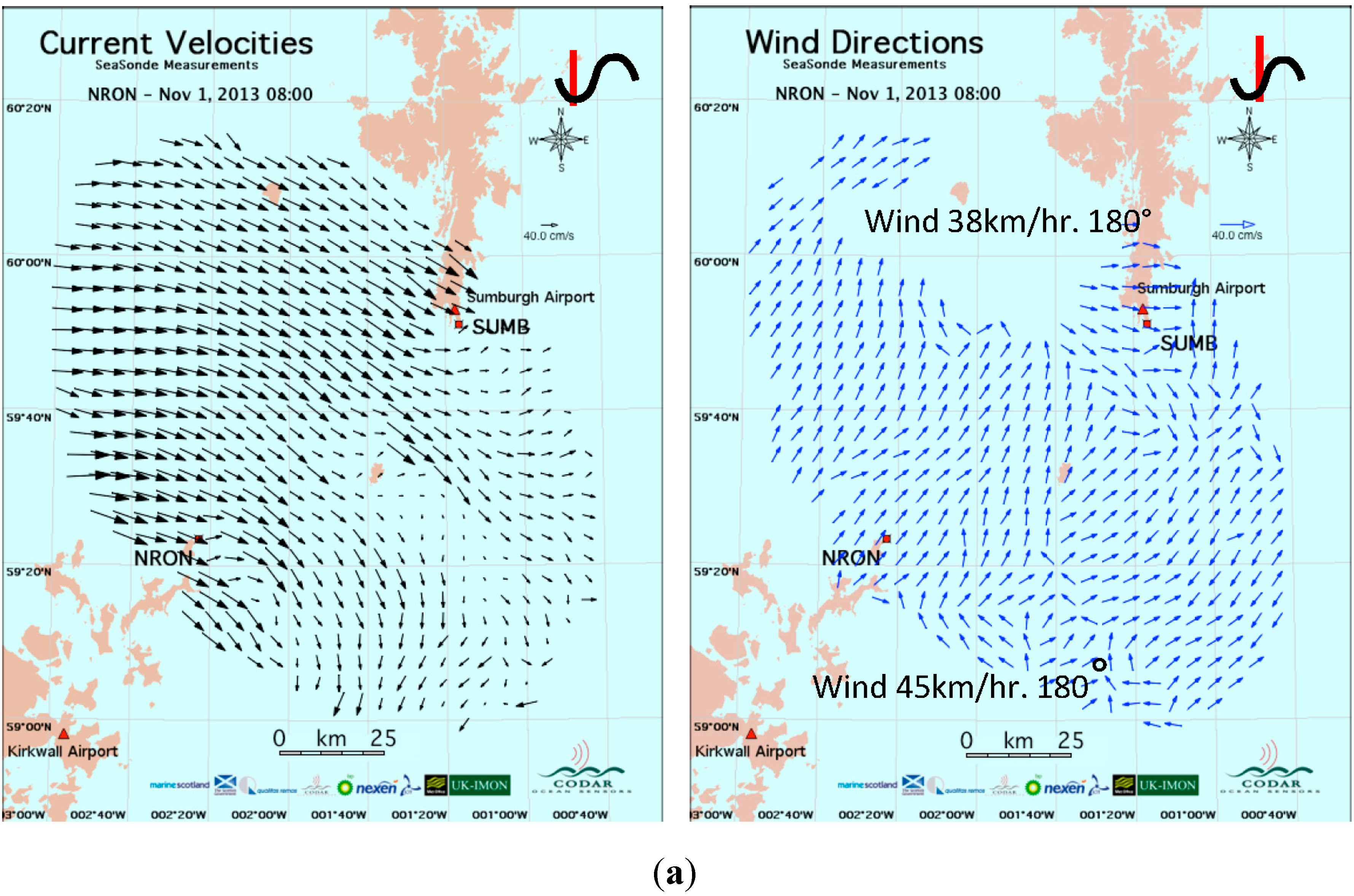
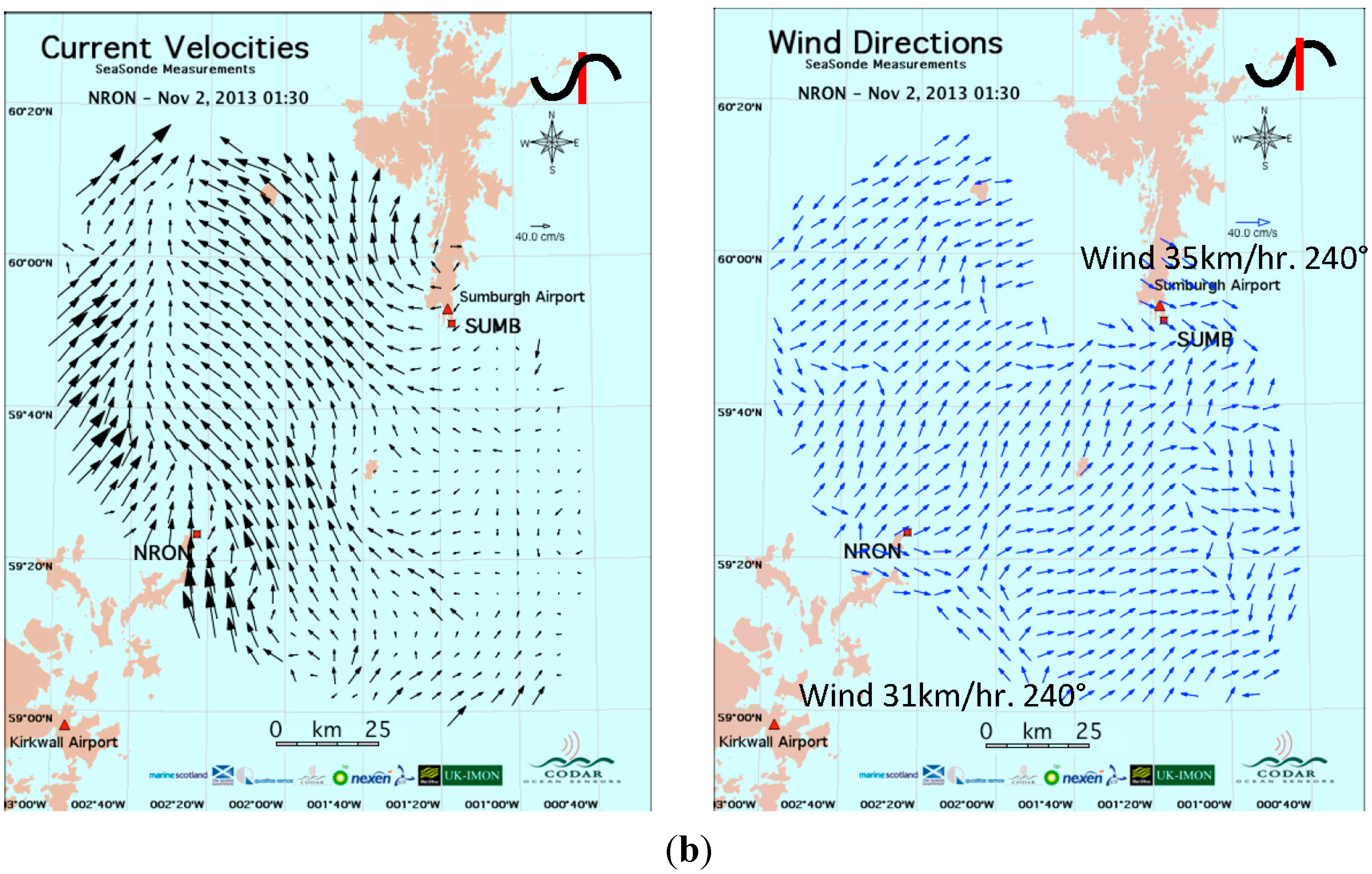
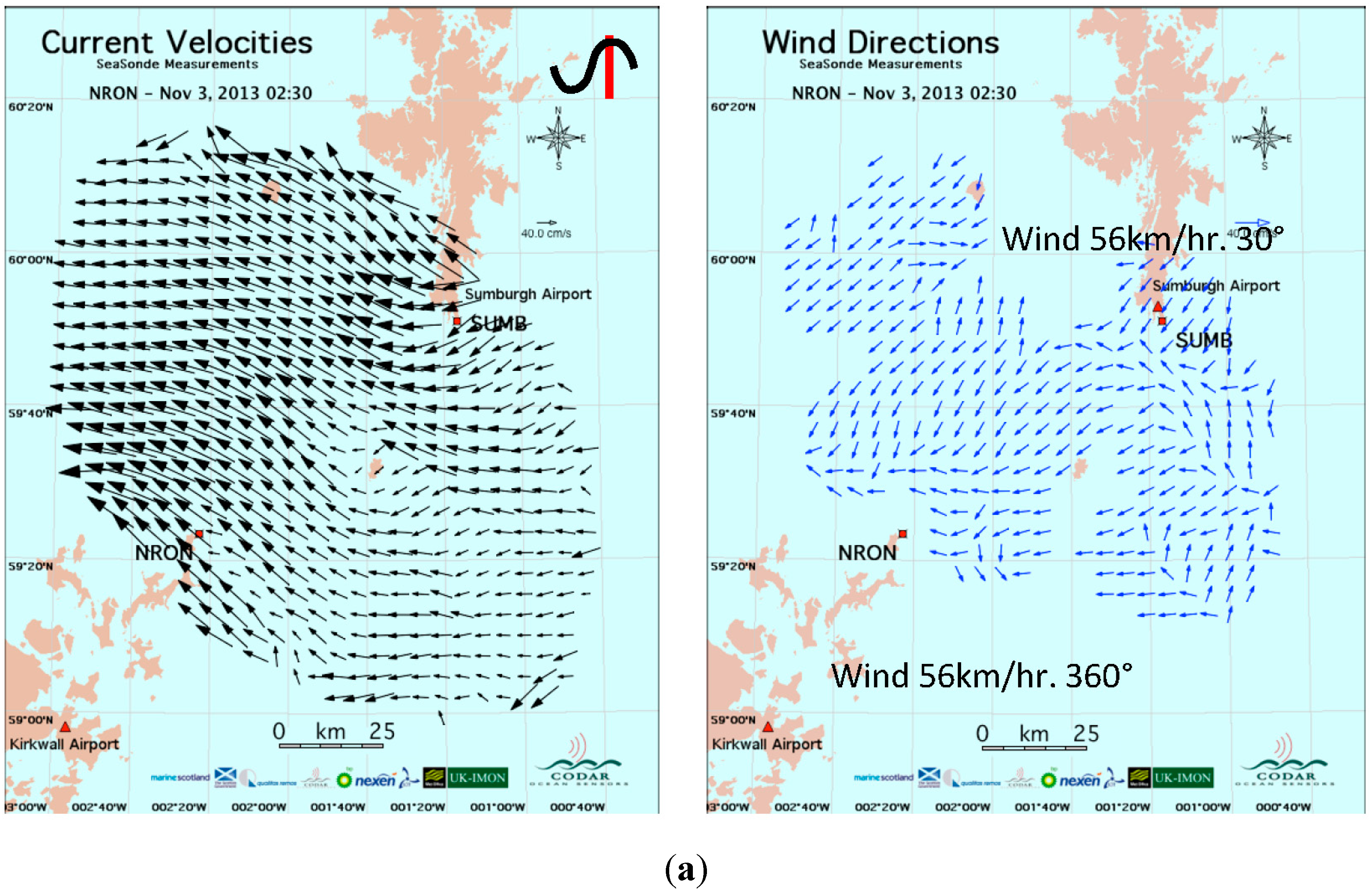
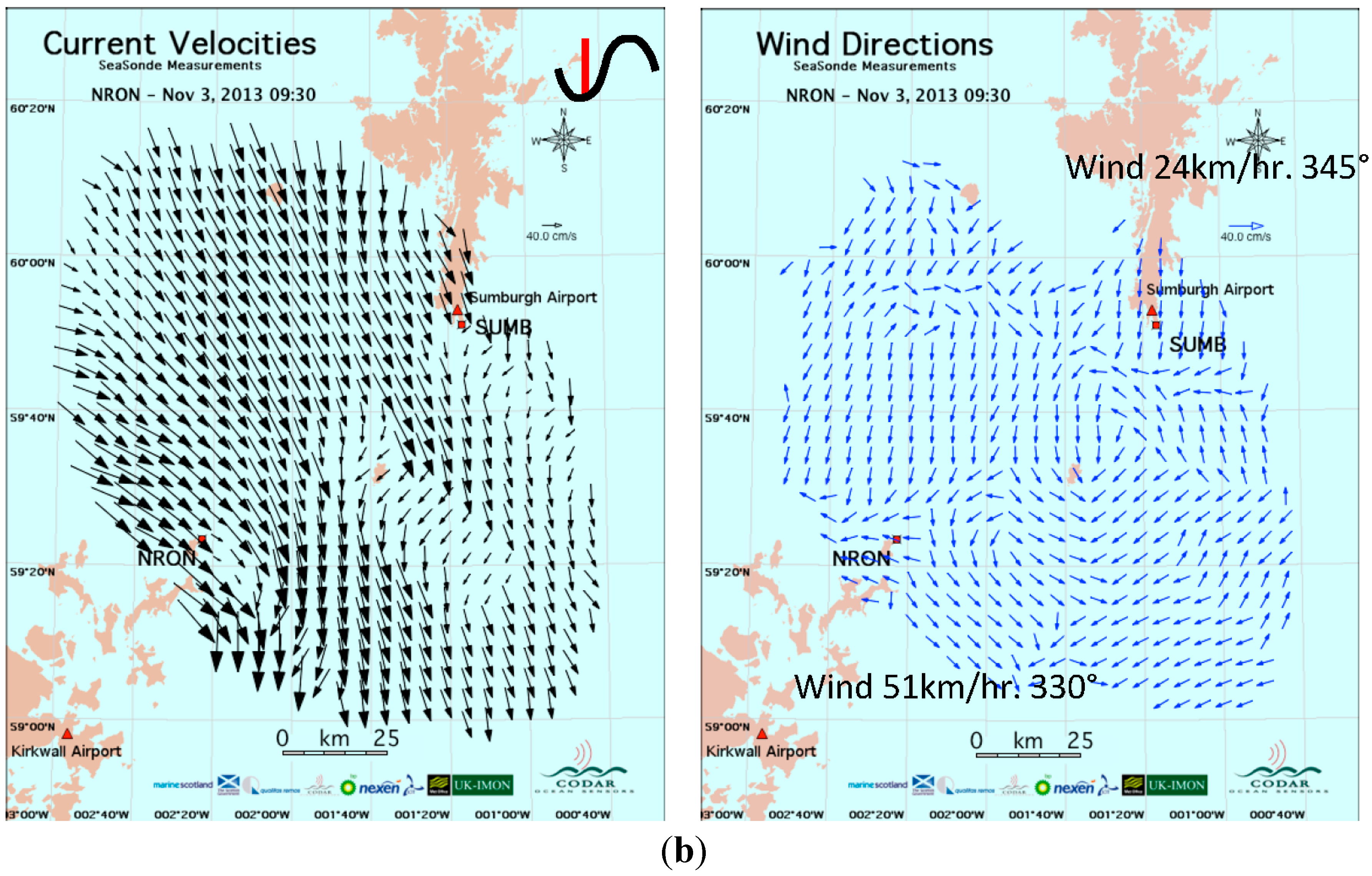
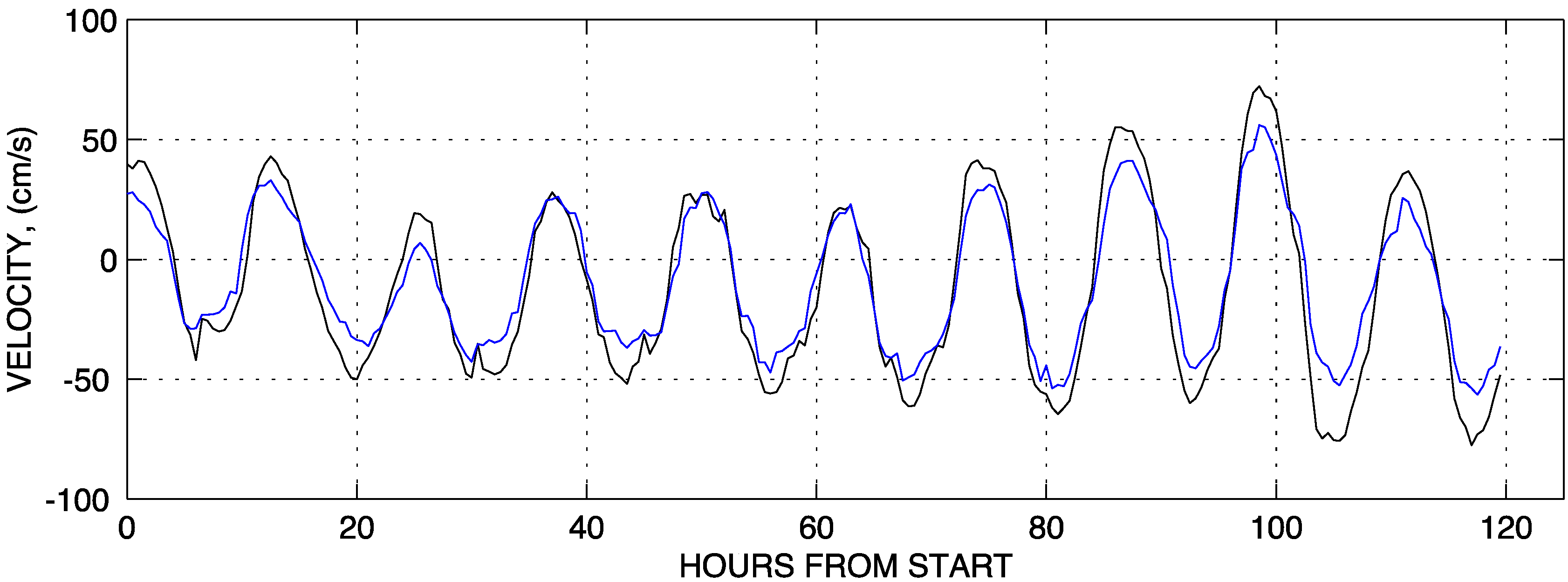
4.1.1. Current Velocity and Wind Direction Maps

The complete set of Brahan current velocity and wind direction maps for the first storm period may be viewed at http://youtu.be/3iVHNtSoHNg.

During this period, the dominant wind direction during the storm was from the SW. Our study of current velocity and wind direction maps shows how strong winds influence the typical surface current flow. As strong winds from the SW continue, they start to affect the typical flow: for example, the typical flow NW→SE veers to the East in the westerly regions, e.g., see Figure 4a. Then, the typical SE→NW flow in the westerly regions is replaced by flow following the wind from the SW, e.g., see Figure 4b.

Late on November 2, the wind direction changed, veering to the N and then NE. Then, the typical tidal flow resumed NW→SE, e.g., see Figure 5a and SE→NW, e.g., see Figure 5b.

Figure 6 shows the components of the total current velocity vectors from SE to NW averaged over the area contained within the 10th range-cell for the two radars, see Figure 3a, plotted vs. time.

Figure 4. (a) November 1, 2013, 8:00. The SW wind in the westerly region of the map has caused the NW to SE surface flow to veer to the east. (b) November 2, 2013, 1:30. The SE to NW surface flow is replaced by currents from the SW in the westerly region.

Figure 4. (a) November 1, 2013, 8:00. The SW wind in the westerly region of the map has caused the NW to SE surface flow to veer to the east. (b) November 2, 2013, 1:30. The SE to NW surface flow is replaced by currents from the SW in the westerly region.

Figure 5. (a) 3 November 2013, 2:30. The wind has changed direction, now coming mostly from the NE. Typical tidal flow has resumed SE→NW. (b) 3 November 2013, 9:30. Slower winds were now mostly from the NE. Typical tidal flow has resumed NW→SE.

Figure 5. (a) 3 November 2013, 2:30. The wind has changed direction, now coming mostly from the NE. Typical tidal flow has resumed SE→NW. (b) 3 November 2013, 9:30. Slower winds were now mostly from the NE. Typical tidal flow has resumed NW→SE.

Figure 6. Velocity components perpendicular to the baseline between the radar sites, averaged over the area contained within 41km circles (shown in Figure 3), centered on SUMB (blue), NRON (black) vs. hours from October 30, 2013, 00:00 UTC.

Figure 6. Velocity components perpendicular to the baseline between the radar sites, averaged over the area contained within 41km circles (shown in Figure 3), centered on SUMB (blue), NRON (black) vs. hours from October 30, 2013, 00:00 UTC.

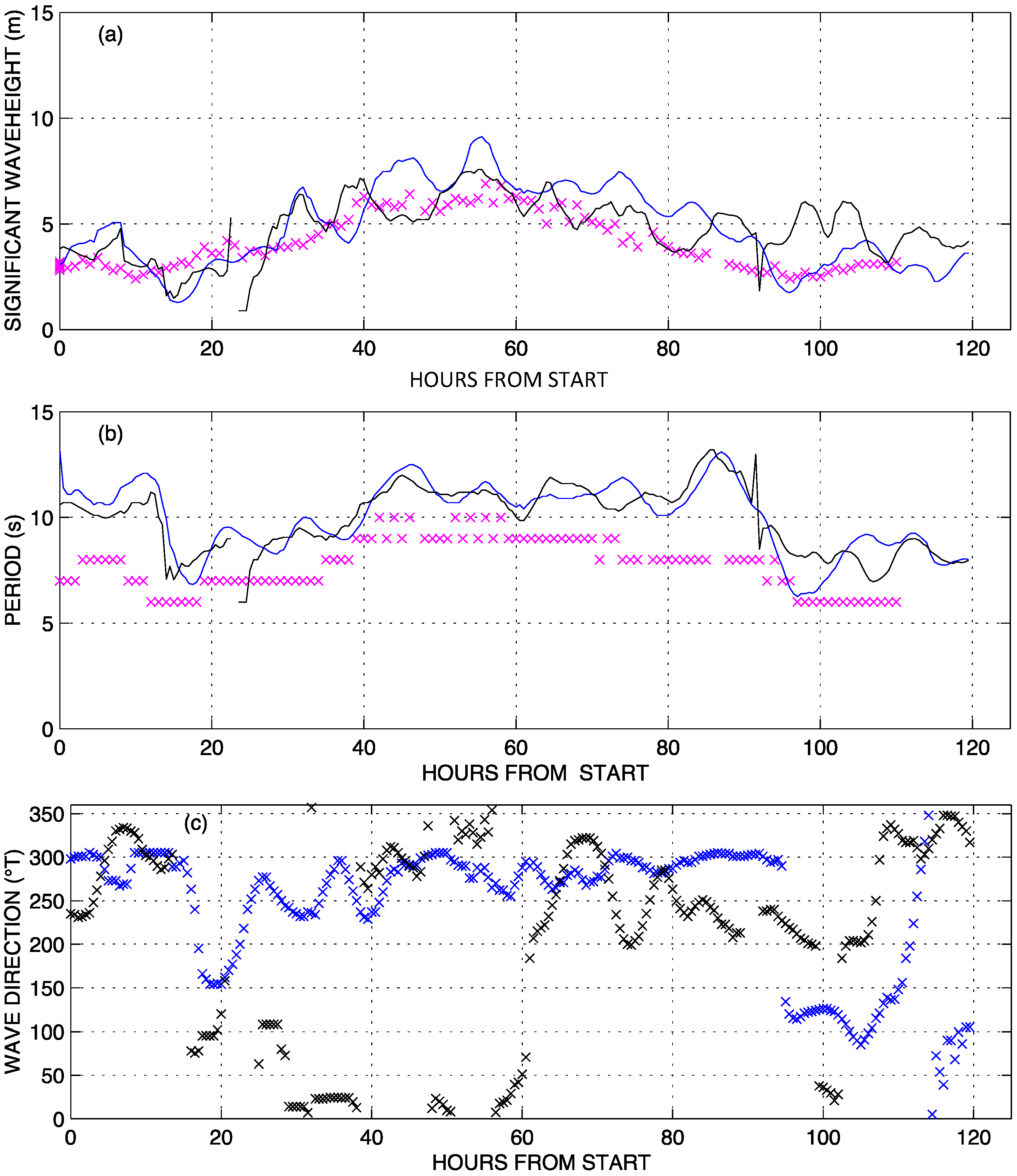
4.1.2. Wave Height, Period and Direction.

These wave parameters were derived using methods described in Section 3.2 and are plotted vs. time for both radars in Figure 7. Figure 7a shows that waveheights increased for 60 hours from about 2 m to a peak of about 7 m and then decreased for 60 hours. Radar-measured waveheights were slightly higher than buoy-measured and exhibit semi-diurnal oscillations. Peaks of the waveheight modulations tend to fall at the troughs of the current velocity waves shown in Figure 6. Figure 7b shows that wave periods increased from about 7 s to 10 s at the peak, then decreased back to 7 s. Figure 7c shows wave directions from the second range-cell indicating considerable differences for the two radars. For SUMB, the wave direction was approximately from the west until around 85 hours, when it started veering to the north. For NRON, the wave direction had a complex pattern, veering between southwest and north. For NRON, we found that the wave direction varied with range, also indicating a complex wave pattern.

Figure 7. (a) Waveheight (b) Wave period (c) Wave directions from range-cell 2 plotted vs. hours from October 30, 2013, 00:00. Blue: SUMB, black: NRON, maroon: Buoy.

Figure 7. (a) Waveheight (b) Wave period (c) Wave directions from range-cell 2 plotted vs. hours from October 30, 2013, 00:00. Blue: SUMB, black: NRON, maroon: Buoy.

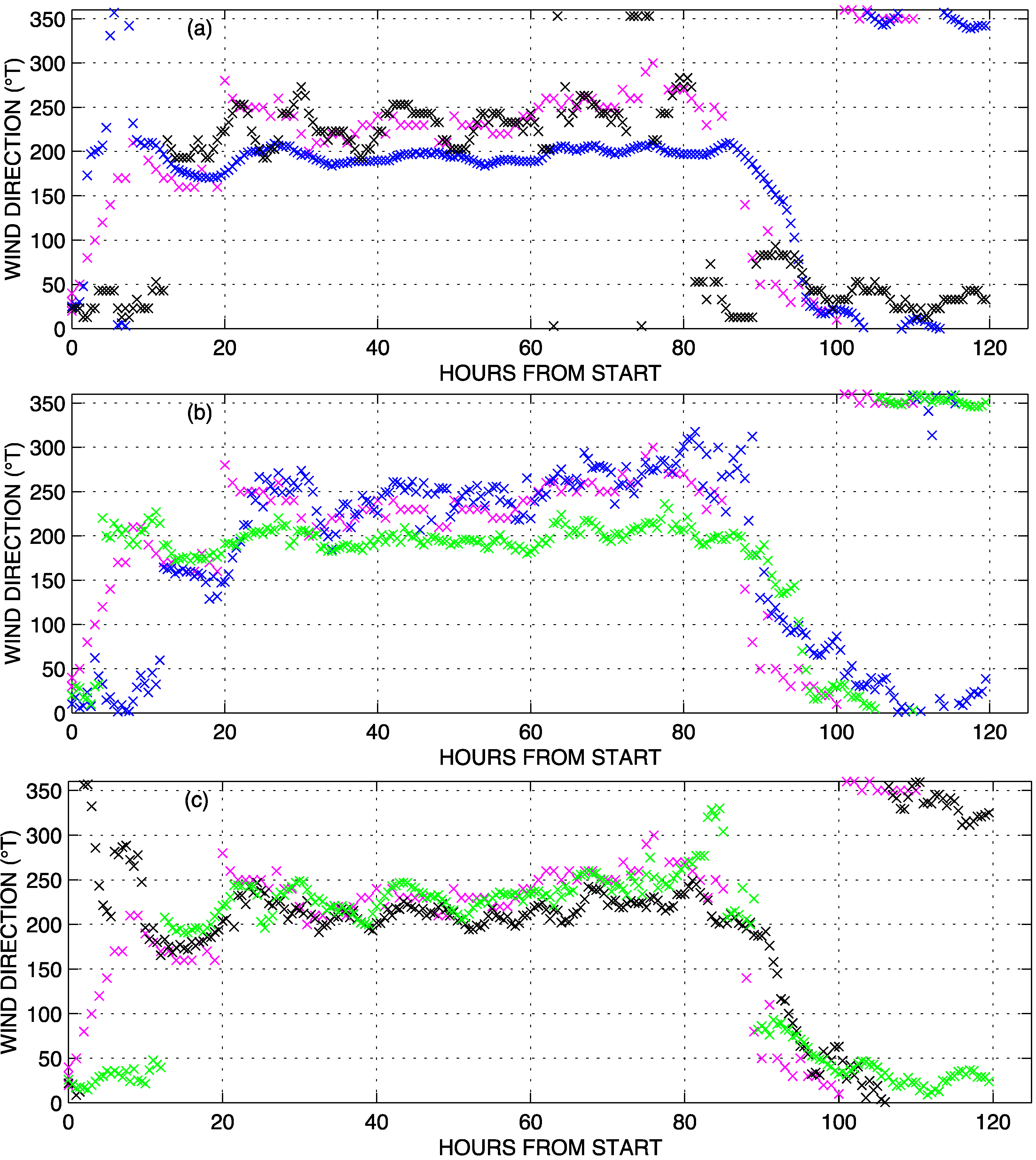
4.1.3. Wind Direction

Wind directions were derived using the two methods described in Section 3.3.

Figure 8a shows results derived from integrated first-order spectra (Section 3.3.1) for range-cell 2. For NRON, the radar-measured wind directions were similar to the buoy-measured directions throughout the storm: from about 50°T at the start, and then from the SW (225°T) for most of the time period, before veering to come from the north at the end. For SUMB, a similar pattern was observed; however, during the bulk of the storm, the waves came from further south, about 190°T. Wind directions from both methods were averaged independently over the area contained within the 10th range-cell, see Figure 3a, for the two radars and the results compared. Figure 8b SUMB: Results from integrated first-order spectra agree with buoy measurements, while those from wind-direction mapping agree with those in Figure 8a from range-cell 2. Figure 8c NRON: Results from integrated first-order spectra and wind-direction mapping are in agreement. They also agree with buoy measurements.

Figure 8. Wind directions plotted vs. hours from 30 October 2013, 00:00: Buoy wind directions: Maroon. (a) Wind directions from integrated first-order energy, Range-cell 2. Blue: SUMB, Black: NRON, (b) Wind directions averaged over the area contained within the 10th SUMB range-cell. Blue: from integrated first-order energy, Green: from wind direction maps. (c) Wind directions averaged over the area contained within the 10th NRON range-cell. Black: from integrated first-order energy, Green: from wind direction maps.

Figure 8. Wind directions plotted vs. hours from 30 October 2013, 00:00: Buoy wind directions: Maroon. (a) Wind directions from integrated first-order energy, Range-cell 2. Blue: SUMB, Black: NRON, (b) Wind directions averaged over the area contained within the 10th SUMB range-cell. Blue: from integrated first-order energy, Green: from wind direction maps. (c) Wind directions averaged over the area contained within the 10th NRON range-cell. Black: from integrated first-order energy, Green: from wind direction maps.

4.2. Results for January 13, 00:00 to January 19, 23:30, 2014 UTC

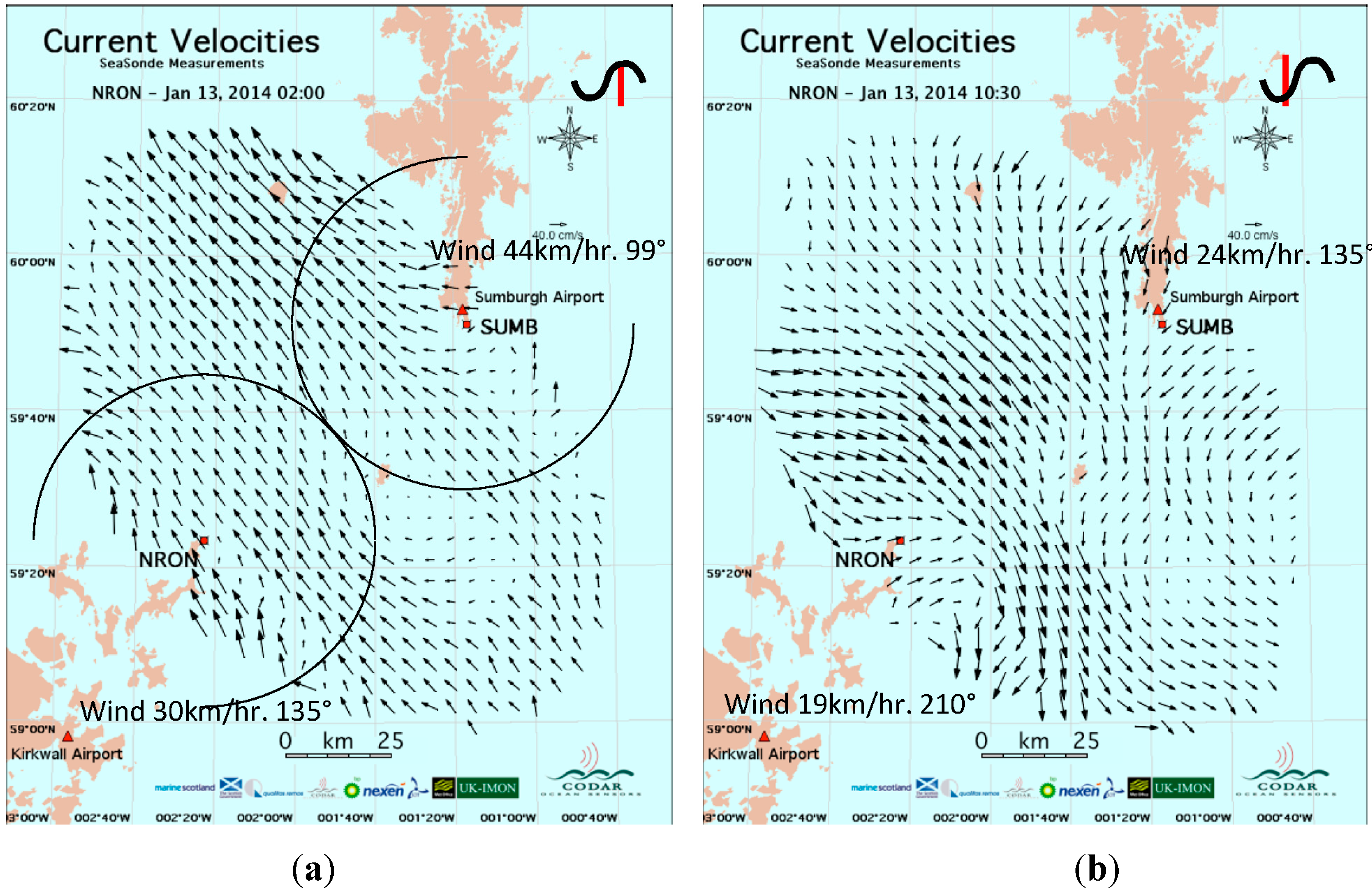
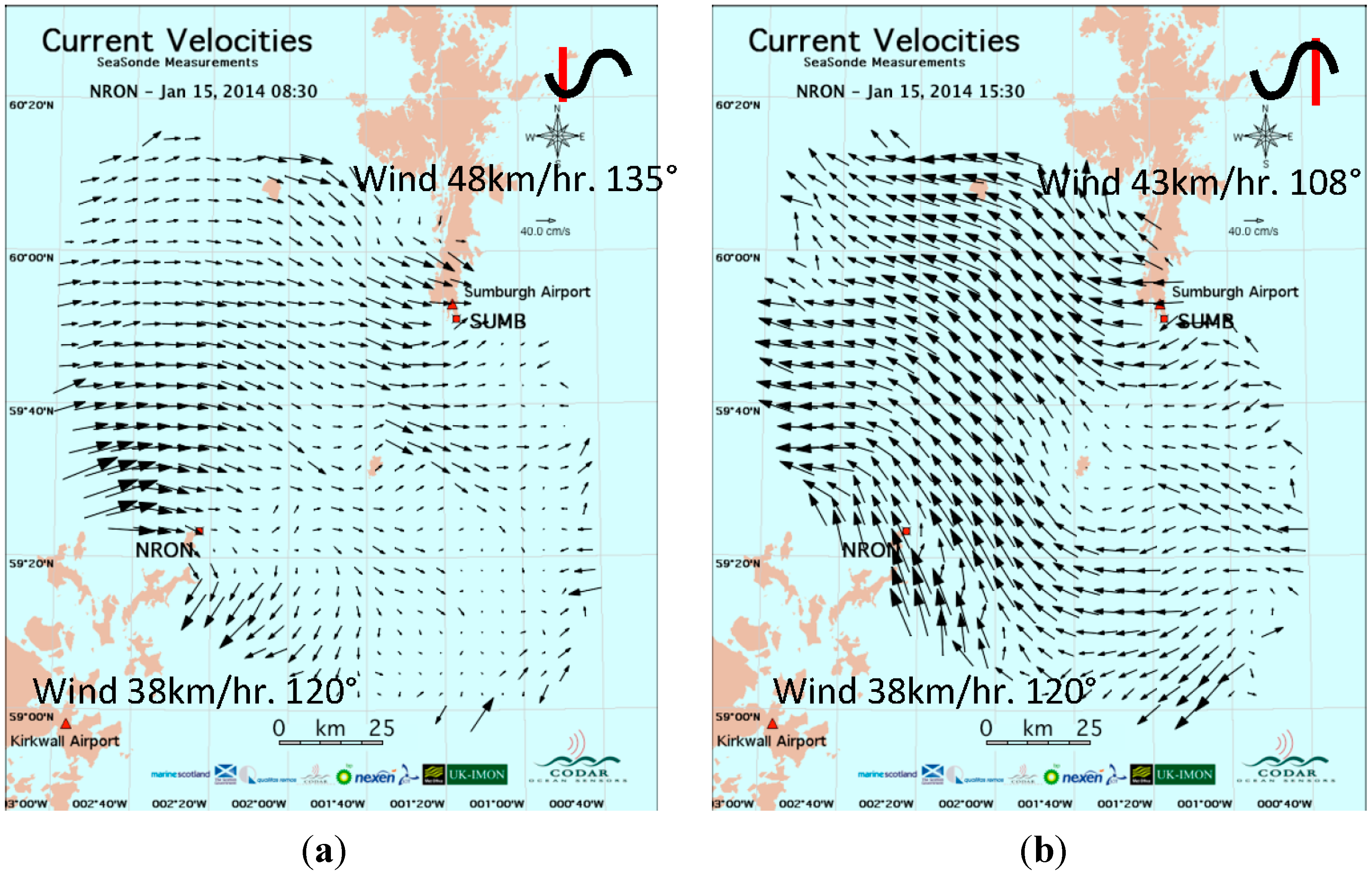
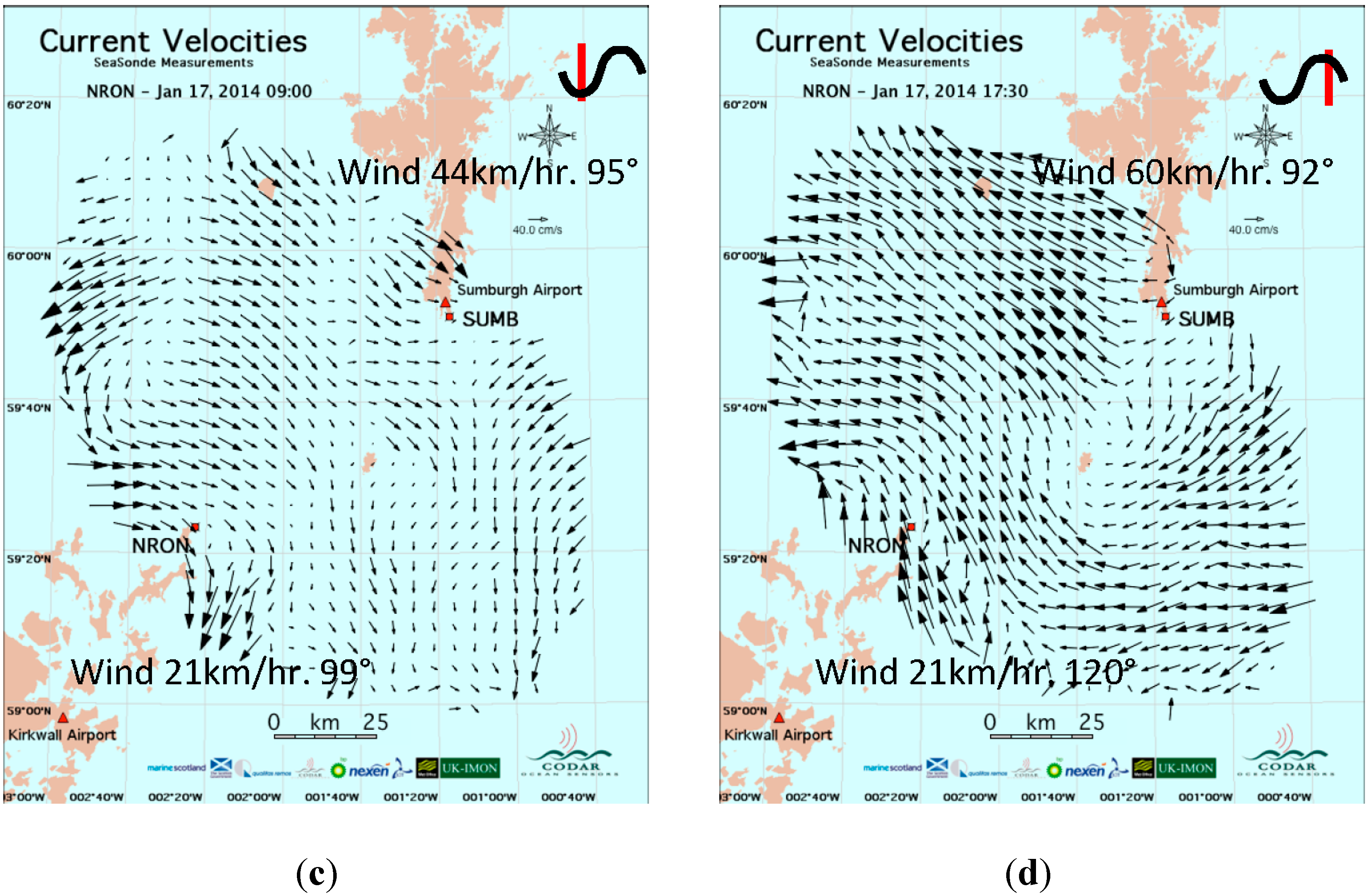
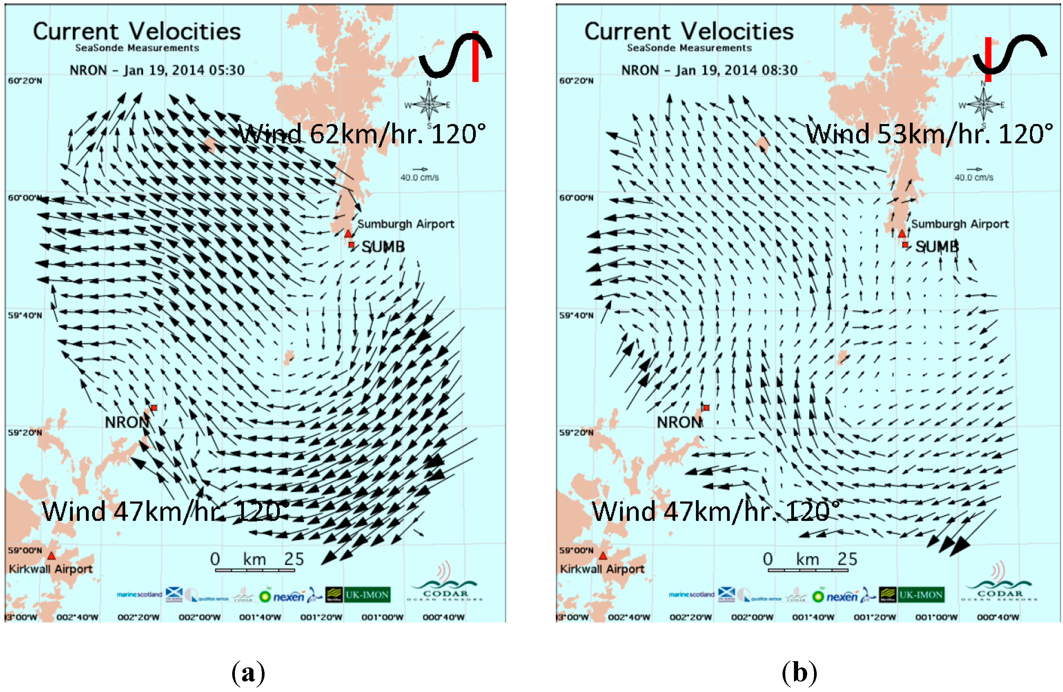
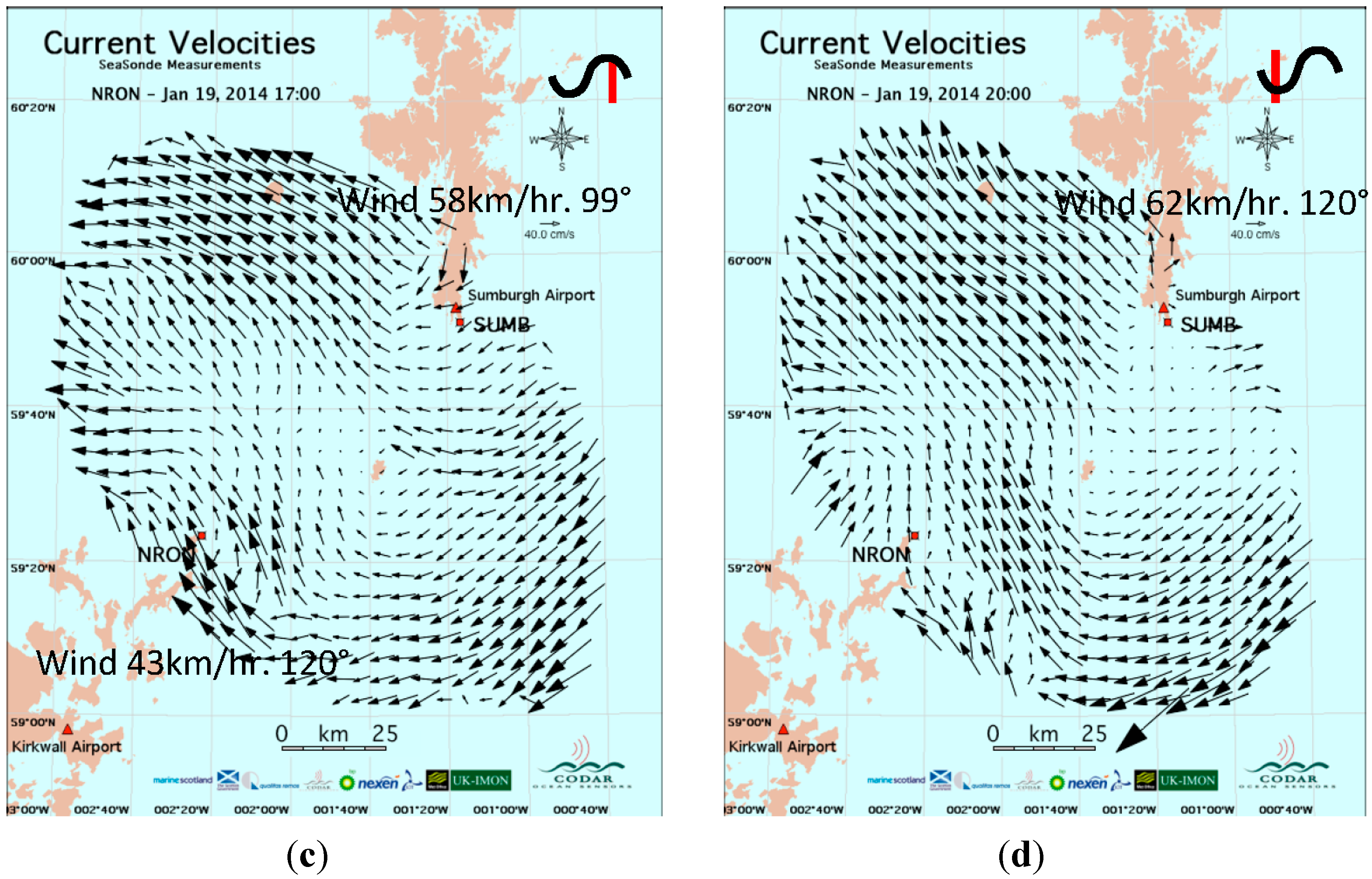
4.2.1. Current Velocity and Wind Direction Maps

Brahan current velocity and wind direction maps for the second storm period may be viewed at http://youtu.be/m4XOPtGY_f4.

The dominant wind direction during this storm was from the SE. At the start of the storm, tides followed the usual pattern consisting of SE→NW tidal flows followed approximately 6 hours later by NW→SE flows, see for example Figure 3.

As the storm continued, the NW→SE the surface flow is weakened from the dominant tidal flow as the opposing prevailing winds from the SE add a wind-driven component, while the SE→NW flow strengthened. Figure 9 gives examples near the January 15 tidal velocity peaks and troughs; Figure 9a shows weakened NW→SE flow; Figure 9b shows strengthened SE→NW flow. By January 17, the weakened NW→SE flow was replaced by complex patterns, e.g., see Figure 9c. Figure 9d shows the start of a circular pattern entering the channel between the islands from the NE that for the rest of the time period dominated tidal flows in the region SE of the baseline joining the radar sites.

Starting late on January 18, the NW→SE flow opposing the wind ceased altogether, and the current pattern seemed to be unrelated to wind direction, tending to be circular, although still modulated by tides; examples close to tidal velocity peaks and troughs are shown in Figure 10. At times near the peak tidal SE→NW flow, Figure 10a,c shows strong flows to the NW in the region NW of the baseline between the radar sites. At times near the peak tidal NW→SE flow, the strong wind from the SE caused reverse SE→NW current flows; see Figure 10b,d. Throughout this time period, in the region SE of the baseline between the radar sites, currents displayed a circular pattern entering the channel from the NE, independent of wind direction.

Figure 9. Current flows near the tidal velocity peaks and troughs showing effects of the strong wind from the SE. (a) January 15, 2014, 8:30 (b) January 15, 2014, 15:30 (c) January 17, 2014, 9:00 (d) January 17, 2014, 17:30.

Figure 9. Current flows near the tidal velocity peaks and troughs showing effects of the strong wind from the SE. (a) January 15, 2014, 8:30 (b) January 15, 2014, 15:30 (c) January 17, 2014, 9:00 (d) January 17, 2014, 17:30.

Figure 10. The circular pattern flow from NE to NW observed from January 18, 2014, 17:30 for the rest of the time period. These examples are for January 19 near the tidal velocity peaks and troughs (a) 5:30 (b) 8:30 (c) 17:00 (d) 20:00 (no data from Kirkwall at this time).

Figure 10. The circular pattern flow from NE to NW observed from January 18, 2014, 17:30 for the rest of the time period. These examples are for January 19 near the tidal velocity peaks and troughs (a) 5:30 (b) 8:30 (c) 17:00 (d) 20:00 (no data from Kirkwall at this time).

Figure 11 shows the components of the total current velocity vectors from SE to NW averaged over the area contained with the 10th range-cell for the two radar sites (see Figure 3(a)) plotted vs. time.

Peak velocities of the oscillations remain approximately constant through the storm, while the trough values tend toward zero near the end, demonstrating the decreasing flow NW→SE opposing the prevailing wind as the storm progressed.

Figure 11. Velocity components perpendicular to the baseline between the radar sites, averaged over the area contained with the 10th range-cell centered on SUMB (blue), NRON (black) plotted vs. hours from January 13, 2014, 00:00 UTC.

Figure 11. Velocity components perpendicular to the baseline between the radar sites, averaged over the area contained with the 10th range-cell centered on SUMB (blue), NRON (black) plotted vs. hours from January 13, 2014, 00:00 UTC.

4.2.2. Wave Height, Period and Direction

During the second storm period, wave heights from both radars steadily increase from about 5 m to about 10 m at the end of the time period, see Figure 12a. Periods for both radars peaked around 20 hours and then increased steadily over the time period from about 7 s to 12 s, see Figure 12b. Wave directions at SUMB were approximately from the E throughout the time period, see Figure 12c, while at NRON, they were approximately from the SE.

Figure 12. (a) Waveheight (b) Wave period (c) Wave directions plotted vs. hours from January 13, 2014, 00:00 UTC . Blue: SUMB, black: NRON.

Figure 12. (a) Waveheight (b) Wave period (c) Wave directions plotted vs. hours from January 13, 2014, 00:00 UTC . Blue: SUMB, black: NRON.

All radar measured parameters exhibit strong semi-diurnal oscillations, particularly NRON, for which the peak-to-trough waveheight magnitude sometimes exceeded 5 m. Peaks of the waveheight modulations tend to fall at the troughs of the current velocity waves. To demonstrate this more clearly, NRON waveheights from Figure 12a and averaged velocity components from Figure 11 are plotted together in Figure 13.

Figure 13. Black: NRON waveheights; Red: averaged velocity components perpendicular to the baseline plotted vs. hours rom January 13, 2014, 00:00.

Figure 13. Black: NRON waveheights; Red: averaged velocity components perpendicular to the baseline plotted vs. hours rom January 13, 2014, 00:00.

4.2.3. Wind Direction

Wind directions were derived using the two methods described in Section 3.3.

Figure 14a shows results for both radars derived from integrated first-order spectra (Section 3.3.1) for range-cell 2. For SUMB, apart from a period before 20 hours, the radar-measured wind directions were similar to the buoy-measured directions, from the SE (approx. 150°T). For NRON, wind directions are from the ENE (approx. 70°T). Wind directions from both methods were independently averaged over the area contained within the 10th range-cell for the two radars and the results compared. Figure 14b SUMB: Wind directions from integrated first-order spectra agree and are from approx. 110°T, while results from wind-direction mapping agree with those in Figure 8a from the buoy (approx. 150°T). Figure 14c NRON: Wind directions from integrated first-order spectra agree with buoy measurements. Results from wind-direction mapping are also in agreement for the bulk of the storm after 40 hours.

Figure 14. Wind directions plotted vs. hours from January 13, 2014, 00:00. Buoy wind directions: Maroon. (a) Wind directions from integrated first-order energy, Range-cell 2. Blue: SUMB, Black: NRON. (b) Wind directions averaged over the area contained within the 10th SUMB range-cell. Blue: from integrated first-order energy, Green: from wind direction maps. (c) Wind directions averaged over the area contained within the 10th NRON range-cell. Black: from integrated first-order energy, Green: from wind direction maps.

Figure 14. Wind directions plotted vs. hours from January 13, 2014, 00:00. Buoy wind directions: Maroon. (a) Wind directions from integrated first-order energy, Range-cell 2. Blue: SUMB, Black: NRON. (b) Wind directions averaged over the area contained within the 10th SUMB range-cell. Blue: from integrated first-order energy, Green: from wind direction maps. (c) Wind directions averaged over the area contained within the 10th NRON range-cell. Black: from integrated first-order energy, Green: from wind direction maps.

4.3. Discussion

Current velocity maps typically show an effect like a shadow SE of the small island near the baseline midpoint, which is especially noticeable for flows from the NW to the SE. The bathymetry shown in Figure 2 indicates there is a shallower seamount around this island that acts to shadow the currents. The seamount diameter and shadow width are about the same.

The Bragg wave direction is usually associated with the wind direction, but for the long-range radars employed in the Brahan Project, the wavelength of the Bragg waves is quite large in comparison with the shorter wavelengths for higher transmit frequencies; wavelength/period are approximately 33 m, 4.6 s. It takes approximately 9 hours duration for 33 m waves to align with the wind and a 120 km fetch is required for full development, see for example http://www.tpub.com/weather3/1-2.htm. Therefore, the association with wind direction is not always valid. For example, it can be seen in Figure 14a that Bragg waves do not follow the veering wind from 10:00 to 23:30, 13 January 2014. The wind speed was low at this time [13,14]. Averaged wind directions shown in Figure 14b,c do indicate that Bragg waves may be following the wind at greater ranges, probably because of higher wind speeds.

Consistency checks between the two methods using further area averaging show agreement within about 40° for SUMB and about 10° for NRON. Some variability is to be expected, because wind direction maps show complex patterns. Also the two methods for deriving wind direction described in Section 3 involve analysis of data from different areas: The first method (see Section 3.3.1) involves analysis of integrated first-order spectral energy from a 4.1 km circular annulus centered on the radar; derived wind directions show considerable variation with range. The second method (see Section 3.3.2) involves analysis of data obtained from a 15 km circle centered on grid points over the radar coverage area.

5. Interpretation of Observed Semi-Diurnal Wave Modulations

5.1. Previous Wave-Current Interaction Studies

Our finding of wave parameter modulations aligning with the strong semi-diurnal tidal current velocities was initially unexpected. However, the literature has a rich history of wave-current interaction hydrodynamics, going back into the early 1940s. Reviews of these early works and their problems can be found in Longuet-Higgins and Stewart [16,17]. They treated both gravity-driven tides and surface waves as propagating wave fields, using perturbation theory to carry the nonlinear expansions to second-order. They found that the shorter surface waves coupled to tidal velocities in the second-order terms and explained inconsistencies in earlier works on the subject. However, their analyses treated water of constant depth and furthermore, the requirements for their analysis to be valid fail for many practical ocean site conditions, including those in the area monitored during the Brahan Project. Spatial variations of tidal currents along the paths of the surface gravity waves are important in explaining the coupling that was subsequently observed. Vincent [18] built upon their work, examining observations in the southern North Sea, but found inconsistencies which he attributed to depth variations not accounted for in the derivation.

Tolman [19,20] derived closed-form relations valid over short space/time scales and also attempted to explain observations in the North Sea. He used the principle of conservation of wave action, following Phillips [21]. He allowed depth to vary, but found that his theoretical results for wave height modulation were not always consistent, which he attributed to errors dominating current-induced changes. At another North Sea location, he suggested that mean wave-height changes may be wind- rather than tide-dominated.

Masson [22] presents a particularly relevant example of tidal modulation of wave parameters, supported by both measurements and theoretical arguments, which we will now summarize and compare with our observations.

5.2. Theory of Wave Oscillations

Masson [22] derived a linear model for the interaction of tidal currents with surface gravity waves based on conservation of wave action, following Huang et al. [23]. This model, with simplified assumptions of uniform flows over small spatial areas, gives the following estimate for the ratio of the waveheight temporal energy spectrum as modified by tidal flows, $E(\omega )$, to the waveheight energy spectrum in deep water in the absence of tidal current flow, $E_0(\omega )$:

$$\frac{E(\omega )}{E_0(\omega )} = \frac{4}{{\left[1+\sqrt{1+ \frac{4U_w\omega }{g}}\right]}^2\sqrt{1+ \frac{4U_w\omega }{g}}}$$

(8)

where $\omega$ is the radian frequency that includes the Doppler shift of the gravity wave train due to current velocity, $U_w$ is the time-varying tidal current velocity component in the direction of wave propagation, and $g$ is the acceleration of gravity. $U_w$ is positive when the current and wave velocities are in the same direction, and negative when they oppose each other.

The radian frequency $\omega$ is given in terms of the radian temporal frequency $\sigma$ of the gravity wave and the deep-water wavenumber k as:

$$\omega =k{U}_w+ \sigma$$

(9)

where $\sigma$ is related to k by the dispersion relation:

$${\sigma }^2=gk$$

(10)

when the wave and current velocities oppose each other such that $U_w$ is negative, the denominator of (8) can approach zero as $\frac{4U_w\omega }{g}$ approaches −1, when the right hand side of Equation (8) approaches infinity.

This has the physical meaning that the velocity of the tidal current and the group velocity of the surface gravity wave are equal and opposite, implying that standing waves are generated. As this begins to happen, the wave steepens and its height increases. Thus, the wave heights on an opposing tidal flow increase, whereas, they decrease when the wave and tidal velocities are in the same direction. In practice, this “singularity” is never reached, because the steepening causes wave breaking, a nonlinear dissipation of energy. In the cases treated in this paper and in [22], velocities are well away from this singular condition.

Equation (8) provides an adequate representation of E(ω) only when the lower wave frequencies are well below the singularity value. Then, it provides an approximate estimate of changes in wave amplitude produced by tides, giving a rough estimate of the change in wave-energy spectral maximum due to a varying tidal current U_w as it swings from positive to negative along the dominant wave direction. The total spectral energy fluctuates with this peak amplitude, when second-order changes in wave spectral width are ignored.

The fractional change in the integrated energy spectra can be related to that in waveheight as follows:

$$\frac{{\displaystyle \int }E(\omega )\text{d}\omega -{\displaystyle \int }{E}_0(\omega )\text{d}\omega }{{\displaystyle \int }{E}_0(\omega )\text{d}\omega } = \frac{h^2-h_0^2}{h_0^2} = \frac{(h-h_0)(h+h_0)}{h_0^2}$$

(11)

where the waveheights h, h₀ are given by the square roots of the corresponding integrated energy spectra. For small velocity deviations, when $\text{Δ}h= (h-h_0) <<h$ we can write the following approximate relationship.

$$\frac{(h-h_0)(h+h_0)}{h_0^2}\approx \frac{2\text{Δ}h}{h_0}$$

(12)

5.3. Comparison of Theory and Observations

Based on the theory described in Section 5.2, we obtained estimates of the magnitude of waveheight modulations for comparison with measured values. During the two storm periods studied, typical wave periods observed by the radars were about 10 s, see Figure 7b, Figure 12b, corresponding to a peak frequency of 0.1 Hz in the deep-water spectrum $E_0(\omega )$. Maximum tidal flows are along the SE-NW axis, across the baseline shelf region between the radar sites, see Figure 1. The maximum/minimum velocities are about ±50 cm/s, see Figure 6 and Figure 11. Substituting these values into Equations (11) and (12) gives an approximate 14% peak-trough variation in waveheight about the mean. Figure 7a and Figure 12a show that the varying wave height modulation temporal variations sometimes exceed this amount, but at other times are less. On average, measured modulations seem to exceed our calculated estimate.

5.4. Discussion

Wave parameters (height, period, direction) shown in Figure 7, Figure 12 and the Bragg wave direction shown in Figure 8, Figure 14 often show significant, in-phase oscillations that are believed to be due to a hydrodynamic semi-diurnal tidal-current modulation. These oscillations were stronger for the second time period, perhaps because the waveheight was larger then. It appears unlikely that the observed oscillations in wind directions inferred from the Bragg waves are actually due to wind variations, but are due to hydrodynamic water-wave modulations. This is supported by Figure 7c, Figure 8 and Figure 12c, Figure 14: During periods when the semi-diurnal wave modulation for wave direction is weak, it is weak also for the Bragg wave direction. Tidal modulation of waves occurs mostly at high latitudes where tidal currents are strong and wave heights are significant. Tidal currents and wave-modulation forcing strengthen when they flow from a deep region, up over a shallower shelf, and then back again into deep water. Tidally-forced modulations are strongest when the tidal current and wave dominant directions are co-linear. Both measurements and theory show that the strongest modulations occur when tidal currents and waves oppose each other. Theoretical predictions of modulations from calculations are somewhat weaker than actual measurements, indicating that other coupling mechanisms exist.

Measurements described in [22] were made in a region south of the Queen Charlotte Islands in the Eastern Pacific, at a latitude close to that of Brahan. It also had moderately strong tides and a bar of shallower water over which tidal flows strengthened, surrounded by deeper water; similar to that between the radar sites at Brahan, see Figure 2. Significant semi-diurnal modulations of waveheight were observed where the water was shallower (115 m), measured by WaveRider non-directional buoys, while a second such buoy in 300 m water showed negligible wave height variations. In our case, waveheight oscillations were observed in the shallow water close to the radars, while the U.K. Met Buoy in deep water to the Northwest (see Figure 2) saw no periodic variations. Similarly to our results, Masson [22] found that measured modulations seem to exceed the calculated estimates, and obtained approximately the same percent modulation. Waveheight fluctuations were measured with a wave buoy. In our case, they were extracted from the HF radar second-order echo. Thus, both sets of measurements, with different instruments in different oceans, saw the same phenomena under similar tidal conditions and were supported by the same hydrodynamic model leading to Equation (11).

6. Conclusions

We have presented wind-direction maps produced by a pair of SeaSondes, which show a strong and unexpected spatial variability. SeaSonde wind-direction mapping is in a preliminary stage. Before full acceptance, wind-direction mapping needs to be verified by sensors making simultaneous observations at different points in the mapping area over a significant period of time.

This paper focuses on two major storm periods, looking at current patterns, wave parameters, local wind direction near each of the two sites, and wind direction maps based on both sites. It demonstrates the comprehensive information available from HF radar observations. Methods, results and interpretation are described and the interaction between different ocean observables is discussed. In particular, periodic time oscillations are seen in the wave parameters that are believed to be forced by the semi-diurnal tides flowing across the shallow shelf between the Orkneys and Shetlands. Theoretical hydrodynamic analysis supporting tidal forcing of waves is presented and results for waveheight modulation compared with prediction. This semi-diurnal periodicity has never been observed before with HF radars.

References and Notes

1. Brahan SeaSonde HF Radar Project. Available online: http://www.thebrahanproject.com/ (access on 3 December 2014).
2. Kohut, J; Roarty, H.; Glenn, S. Characterizing observed environmental variability with HF Doppler radar surface current mappers and acoustic Doppler current profilers: Environmental variability in the coastal ocean. IEEE J. Ocean. Eng. 2006, 31, 876–884. [Google Scholar]
3. Hubbard, M.; Barrick, D.; Garfield, N.; Pettigrew, J.; Ohlmann, C.; Gough, M. A new method for estimating High-Frequency Radar error using data from Central San Francisco Bay. Ocean Sci. J. 2013, 48, 105–116. [Google Scholar] [CrossRef]
4. Ohlmann, C.; White, P.; Washburn, L.; Terrill, E.; Emery, B.; Otero, M. Interpretation of coastal HF Radar-derived surface currents with high-resolution drifter data. J. Atmos. Oceanic Tech. 2006, 24, 666–6802. [Google Scholar] [CrossRef]
5. Long, R.; Barrick, D.; Largier, J.; Garfield, N. Wave observations from Central California: SeaSonde systems and in situ wave buoys. J. Sens. 2011. [Google Scholar] [CrossRef]
6. Alfonso, D.; Alvarez, E.; Damian Lopez, J. Comparison of CODAR SeaSonde HF Radar Operational Waves and Currents Measurements with Puertos del Estado Buoys. Final Report. 2006. Available online: http://www.codar.com/images/about/2006PDE_final_Report.pdf (access on 3 December 2014).
7. Lipa, B.; Barrick, D. Least-squares methods for the extraction of surface currents from CODAR crossed-loop data: Application at ARSLOE. IEEE J. Oceanic Eng. 1983, OE-8, 226–253. [Google Scholar]
8. Lipa, B.; Nyden, B.; Ullman, D.; Terrill, E. SeaSonde radial velocities: Derivation and internal consistency. IEEE J. Ocean. Eng. 2006, 31, 850–861. [Google Scholar] [CrossRef]
9. Lipa, B.; Nyden, B. Directional wave information from the SeaSonde. IEEE J. Ocean. Eng. 2005, 30, 221–231. [Google Scholar] [CrossRef]
10. Lipa, B.; Barrick, D. Extraction of sea state from HF radar sea echo: Mathematical theory and modeling. Radio Sci. 1986, 21, 81–100. [Google Scholar] [CrossRef]
11. Fernandez, D.; Graber, H.; Paduan, J.; Barrick, D. Mapping wind direction with HF radar. Oceanography 1997, 10, 93–95. [Google Scholar] [CrossRef]
12. Lipa, B.; Nyden, B.; Barrick, D.; Kohut, J. HF radar sea-echo from shallow water. Sensors 2008, 8, 4611–4635. [Google Scholar] [CrossRef]
13. Weather History for Sumburgh, UK. Available online: http://www.wunderground.com/history/airport/EGPB/2013/11/3/DailyHistory.html (access on 3 December 2014).
14. Weather History for Kirkwall, UK. Available online: http://www.wunderground.com/history/airport/EGPA/2013/11/3/DailyHistory.html (access on 3 December 2014).
15. Station 64046—K7 Buoy. Available online: http://www.ndbc.noaa.gov/station_page.php?station=64046 (access on 3 December 2014).
16. Longuet-Higgins, M.; Stewart, R. Changes in the form of short gravity waves on long waves and tidal currents. J. Fluid Mech. 1960, 8, 565–583. [Google Scholar] [CrossRef]
17. Longuet-Higgins, M.; Stewart, R. Changes in the form of short gravity waves on Steady nonuniform currents. J. Fluid Mech. 1961, 10, 529–549. [Google Scholar] [CrossRef]
18. Vincent, C. The interaction of wind-generated sea waves with tidal currents. J. Phys. Oceanogr. 1978, 9, 748–755. [Google Scholar] [CrossRef]
19. Tolman, H. The influence of unsteady depths and currents of tides on wind-wave propagation in shelf seas. J. Phys. Oceanogr. 1990, 20, 1166–1174. [Google Scholar] [CrossRef]
20. Tolman, H. Effects of tides and storm surges on North Sea wind waves. J. Phys. Oceanogr. 1991, 21, 766–781. [Google Scholar] [CrossRef]
21. Phillips, O.M. The Dynamics of the Upper Ocean, 2nd ed.; Cambridge University Press: New York, NY, USA, 1997. [Google Scholar]
22. Masson, D. A case study of wave–current interaction in a strong tidal current. J. Phys. Oceanogr. 1996, 26, 359–372. [Google Scholar] [CrossRef]
23. Huang, N.; Chen, D.; Tang, C. Interactions between steady nonuniform currents and gravity waves with applications for current measurements. J. Phys. Oceanogr. 1972, 2, 420–431. [Google Scholar] [CrossRef]