
On-Orbit Relative Radiometric Calibration of the Bayer Pattern Push-Broom Sensor for Zhuhai-1 Video Satellites


1
College of Urban and Environmental Sciences, Hubei Normal University, Huangshi 435002, China
2
College of Computer Science and Technology (CCST), Zhejiang University, Hangzhou 310058, China
3
Institute of Remote Sensing Satellite, China Academy of Space Technology (CAST), Beijing 100094, China
4
Wuhan Jiangshantuhua Engineering Technology Co., Ltd., Wuhan 430074, China
5
School of Remote Sensing and Information Engineering, Wuhan University, Wuhan 430079, China
6
State Key Laboratory of Information Engineering in Surveying, Mapping and Remote Sensing, Wuhan University, Wuhan 430079, China
7
Zhuhai Orbita Aerospace Science & Technology Co., Ltd., Zhuhai 519080, China
*
Author to whom correspondence should be addressed.
Remote Sens. 2023, 15(2), 377; https://doi.org/10.3390/rs15020377
Submission received: 30 November 2022
/
Revised: 27 December 2022
/
Accepted: 6 January 2023
/
Published: 7 January 2023
(This article belongs to the Topic Micro/Nano Satellite Technology, Systems and Components)
Abstract
:The two video satellites of the second and third batch of Zhuhai-1 microsatellites (referred to as OVS-2A/3A) are operational with their hyperspectral satellites, which improves the data acquisi-tion capability of the Zhuhai-1 remote sensing satellite constellation. Contrary to the linear array push-broom hyperspectral satellites and plane array CCD video satellites, the OVS satellite is equipped with a planar array Bayer pattern sensor, which can obtain single-band grayscale images by push-broom imaging. Additionally, the Bayer color reconstruction algorithm can interpolate sensor data to provide RGB color band information. Therefore, for the Bayer pattern push-broom sensor, the relative calibration method of linear push-broom or array cameras cannot be directly applied. The radiometric calibration of the Bayer pattern push-broom imaging mode has become a matter of concern; therefore, this study developed a radiometric calibration method for the Bayer pattern push-broom sensor of the OVS satellite and verified its effectiveness and accuracy. OVS images were used to perform on-orbit relative radiometric calibration, and the calibration accu-racy, including streaking metrics and root-mean-square error, was better than 1%, meeting the specification requirements for the OVS satellite. Visually, after calibration correction, the streaking and striping noise of the Bayer images was removed, and the radiometric quality of the image was considerably improved, providing a good data basis for subsequent research in remote sensing applications.
1. Introduction
Adherence to the “single satellite with multiple functions” concept has greatly improved the image acquisition capability of single remote sensing satellites and expanded the scope of their application, which has resulted in the widespread usage of single remote sensing satellites for scientific research and commercial applications. Micro and low-cost commercial remote sensing satellites, such as the two video microsatellites (OVS-2A/3A) of the Zhuhai-1 satellite constellation, which have both video and linear array push-broom satellite imaging capabilities, can acquire dynamic video data and push-broom long strip data.
1.1. OVS Satellites Overview
The OVS satellites are equipped with five plane array Bayer pattern CMOS sensors with resolutions of 0.9 m, arranged in an up-and-down staggered pattern (Figure 1a), and 50 detectors overlapped between different CMOS sensors. The single CMOS has 5056 (H) × 2968 (V) detectors and the Bayer pattern for CMOS1,3,5 is a “GBRG” pattern (Figure 1b) and for CMOS2,4 is a “GRBG” Bayer pattern (Figure 1c). Detailed information for the sensor is shown in Table 1.
For the Bayer pattern sensor, only one color is captured by each detector during imaging, and the full red, green, and blue (RGB) three-color band information at each detector must be reconstructed by the Bayer interpolation algorithm in the ground image processing system (Figure 2a). A major advantage of the Bayer pattern sensor over conventional multispectral sensors is that the amount of data acquired is drastically reduced while the image color information is retained (Figure 2b); hence, they are more commonly used in video and low-cost micro remote sensing satellites and can expand the scope of application of image data, such as ship detection [1].
The OVS satellite uses a Bayer pattern sensor to provide two imaging modes: the staring and push-broom modes. The staring mode uses all plane array detectors to focus on an individual target (Figure 3a) and can obtain 8 bits of video data with a frame rate of approximately 10–25 fps. The push-broom mode uses the Bayer partial row detectors to form multilevel time delay integration (TDI), which is then used to perform push-broom imaging along the flight direction of the satellite to obtain 10 bits of long strip data, as shown in Figure 3b. For OVS satellites, approximately 17,000 km2 of data can be captured in each strip image. Contrary to the conventional linear push-broom mode, the Bayer pattern push-broom mode uses the Bayer pattern detector group, which utilizes two rows of imaging detectors as the smallest imaging unit. This achieves the same multi-level TDI function as the linear array push-broom satellite by increasing or decreasing the number of Bayer pattern rows. Figure 4 shows a comparison of a conventional linear array push-broom and a Bayer pattern push-broom. The imaging data in the push-broom direction is the imaging data collected by a single detector in a single band, while the Bayer pattern push-broom obtains data from multiple bands.
1.2. Relative Radiometric Calibration
The Bayer pattern sensor of OVS satellites has 5056 × 2968 detectors, each of which has its own unique physical properties, such as size and filter performance, which has resulted in detector response inconsistency, non-uniform electronic sensor biases, inconsistencies in the fixed-noise and dark current, and differences in the output circuit. Therefore, each detector in the sensor that images uniform radiance will output specific digital numbers (DN), resulting in numerous examples of stripe noise in the raw image recorded by the sensor. This degrades image quality and poses a risk to its suitability, which is required for analysis (Figure 5a). Relative radiometric calibration aims to calibrate inconsistencies in terms of sensor detector responses, eliminating detector-level striping artifacts (Figure 5c). When Bayer sensors lack relative radiometric calibration, their direct color interpolation may produce incorrect results. Figure 5b shows that the Bayer color interpolation algorithm enhances detector-level errors in raw Bayer pattern data, disturbing interband color information. Figure 5c shows the visual effect of Bayer color reconstruction after relative calibration. The RGB color information of a raw Bayer image can be completely covered, indicating that before Bayer interpolation processing, relative radiometric calibration must be performed to eliminate the detector-level radiometric error and improve the image quality of the Bayer color reconstruction image.
Several radiometric calibration and correction methods have been widely developed by researchers to reduce these radiometric errors [2,3,4,5,6]. OVS satellites are low-cost microsatellites and are not equipped with on-board calibration equipment. Therefore, a calibration method based on earth images must be selected. In the staring imaging mode for the OVS, the Bayer sensor can be equivalent to the plane array video sensor, and on-orbit relative radiometric calibration can be accomplished using the sequence frame data, such as the uniform filed calibration of the SkySat satellites [7], LuoJia1-01 satellite [8], and calibration without the uniform filed data of Jilin video satellites [9]; however, Bayer sensor push-broom imaging differs from the conventional linear push-broom mode because the imaging data in the push-broom direction is collected by a single band, but the Bayer pattern push-broom obtains data from multiple bands. Due to different bands having different radiometric response characteristics, each band of remote sensing sensors must be calibrated independently. The conventional methods include uniform field calibration [10,11], statistical calibration [12,13], yaw calibration [14,15,16], and fieldless calibration [17,18], which are designed for linear push-broom sensors and cannot be directly applied to Bayer pattern sensors. Nevertheless, OVS push-broom imaging characteristics provide a possibility for the relative calibration of the Bayer array push-broom mode by referring to the statistical calibration principle of linear array push-broom remote sensing satellites.
Based on the principle of consistent gray distribution of each imaging detector under the condition of massive samples, this study developed an on-orbit relative radiometric calibration method for the plane array Bayer push-broom imaging mode, which reconstructs the order of each detector within the Bayer pattern sensor and converts it into a virtual linear array sensor to separate the RGB three-band components from the Bayer pattern. For this, a positioning method linked by “linecounters” was designed to detect the specific position of each detector within each Bayer pattern, and a nonlinear calibration model was used to solve the calibration coefficients. These methods are elaborated on in Section 2. Then, in Section 3, the effectiveness of the method is verified based on its visual effect and quantitative evaluation and the calibration accuracy of OVS satellites is evaluated. Lastly, the limitations of calibration methods and radiometric response anomalies of the OVS are described in Section 4.
2. Methods
This method first converts the Bayer pattern into a virtual linear array sensor and counts the gray scale distribution curves of the imaging samples for each virtual detector of the virtual linear array sensor. According to the statistical calibration principle, when the imaging sample number is sufficient, the imaging gray scale distribution curves of each detector within the virtual linear array sensor are consistent. The variability exhibited by the gray distribution curves was determined by the radiometric response characteristics of each detector. Then, the inconsistency radiometric response error between the detectors was calibrated, and the calibration parameters of each detector within the virtual linear array sensor were solved for based on the histogram statistical principle. Finally, the virtual calibration parameters were converted into Bayer pattern detectors for the relative correction of Bayer images. Therefore, the main technical steps of this method include Bayer pattern conversion, Bayer pattern position determination, and calibration parameter solutions, which are described as follows.
2.1. Bayer Pattern Conversion
As mentioned, the Bayer pattern push-broom imaging of OVS satellites differs from the conventional linear push-broom mode because The imaging data in the push-broom direction is the imaging data of the same detector in the same band, while the Bayer pattern push-broom obtains data in multiple bands. In relative calibration, the imaging data of each detector within each band must be accurately traced to calibrate the radiometric response model of each detector within each band. Therefore, reconstructing the order of each detector within the Bayer pattern sensor and converting it into a virtual linear array sensor is necessary to separate the RGB three-band components from the Bayer pattern.
For OVS satellites using push-broom imaging with a Bayer pattern array, a “GBRG” imaging detector set of the Bayer pattern is equivalent to two green band detectors, one blue band detector, and one red band detector, for a total of four imaging detectors performing push-broom imaging simultaneously. Therefore, two complete rows of the Bayer pattern are converted into one row to form a detector arrangement comparable to the linear array push-broom sensor and referred to as a “virtual linear array push-broom sensor” (Figure 6). The number of probes within the virtual linear sensor imaging detector N is twice the number of probes within the Bayer pattern detector M, where the number of detectors in the R and B bands is half of M, and the number of detectors in the G band is equal to M, as shown in Equation (1).
2.2. Bayer Pattern Position Determination
When a Bayer pattern is converted to a virtual linear sensor, the smallest imaging unit must be complete and cannot be missing; however, owing to the influence of signal occlusion, interference, or rain and snow in the data receiving process, the Bayer pattern image has the phenomena of packet loss, as well as frame and row loss, which destroys the integrity of the Bayer image. Figure 7a shows that, owing to a loss in line 3, the Bayer pattern changed from a pattern of GBRG in lines 3–4 to one of RGGB, and the last row of Bayer pattern data was incomplete (Figure 7b). Therefore, during the calibration process and before Bayer pattern conversion, it is necessary to locate the specific position of each complete Bayer pattern in the image to avoid confusion between separate band detector imaging data and the misalignment of various detector orders in the same band.
A positioning method linked by “linecounters” is designed to detect the specific position of each Bayer pattern. First, a linecounter is added in front of each row of imaging data according to the following rules: (1) when the row data is the first row of the Bayer pattern, the linecounter value is odd, otherwise it is even; (2) a complete Bayer pattern imaging of two rows of data has a continuous linecounter with a difference of 1 [i.e., ; and (3) the linecounters of adjacent Bayer pattern imaging data are consecutive with a difference of 1 [i.e., ] as shown in Figure 8.
The process of determining the location of the complete Bayer pattern according to the above rules is as follows:
- 1.
- Calculate the linecounter value of the ith row of Bayer pattern data.
- 2.
- Determine the first position of a complete Bayer pattern. If is odd, the following equation holds:where the ith row data is the starting line of the Bayer pattern. If this is true, then the order can proceed to step (3), otherwise the calculation must be performed before returning to step (1).
- 3.
- Determine whether the ith row Bayer pattern data is continuous with the adjacent imaging data and Bayer pattern according to the following rules:If the ith iteration meets the above formula, the ith row is the starting row of the complete Bayer pattern data. Otherwise, the ith data will be discarded and the calculation must be performed before returning to step (1).
- 4.
- Repeat steps 1–3 to determine the locations of all complete Bayer pattern data.
2.3. Relative Calibration Parameter Solving
The statistical calibration principle can be applied to the virtual linear array sensor constructed from the original Bayer pattern. The probability distribution of scene DN values acquired by each detector is the same when there are enough imaging samples. The variability in the probability distribution of DNs across the detectors is caused by the inconsistent radiometric response of the detectors. For the discrete quantization of the optical remote sensing satellite sensor, the specific process is as follows:
- 5.
- Calculate the DN number of the imaging data acquired by the ith detector, as in the following equations:where , n is sensor quantization bits, is the number of DNs whose value of the ith detector of the virtual linear sensor is equal to k. is the total number of DNs acquired by the ith detector of the virtual linear array.
- 6.
- Establish the cumulative probability distribution function, , of each sensor detector according to Equation (7).
- 7.
- 8.
- Set the cumulative probability distribution function of the imaging gray data of all the sensor detectors as the reference cumulative probability distribution function for each band, ,, and :where is the total number of the virtual linear array sensor detectors.
- 9.
- Obtain the imaging response model of each sensor detector by mapping the cumulative probability distribution function of each sensor detector to the reference cumulative probability distribution function based on Equations (11) and (12):where k is the current calibration gray-level, the range of values of x and y is , and n is the satellite sensor image quantization bit.
The relative calibration parameters obtained from steps 1–4 are the maps of the imaging DN values from each detector to the relative corrected DN values. The relative radiometric correction is achieved by locating each detector according to the Bayer pattern conversion and position determination rules from Section 2.1 and Section 2.2, and the imaging DNs of each detector are then mapped to the new DNs based on the relative calibration parameters. This is an effective method to solve the non-linear calibration model of remote sensing sensors. A one-to-one correspondence between sensor input and output can be established within the sensor quantization range.
2.4. Quality Assessment
Visual assessment is a primary step in assessing the relative calibration quality of images and selecting the bands suitable for analysis. Extending the visual assessment to evaluate the quality of the relative corrected images and recognize and locate the small residual stripes is not new to radiometric calibration or the image processing community. Examples of its use include EO-1 [19], IKONOS [11], and Landsat-8 [15]. For OVS radiometric calibration, we visually assessed and compared the relative calibrated or corrected images. Moreover, profiles drawn at columns across the images before and after correction, in the direction perpendicular to stripes, were used to show the changes in the local brightness levels and reduction in striping.
Meanwhile, as the relative radiometric calibration should eliminate the variations of response between sensors and subjectively judge the effect of image correction, the “streaking metrics” and root-mean-square of the column mean were used in the quantitative analysis to calculate the accuracy of OVS radiometric calibration. The streaking metrics can be used to evaluate the high-frequency response difference of adjacent detectors as follows:
where is the streaking metric of the ith detector in the sensor and is the mean value of the image in the ith detector of the sensor.
The root-mean-square for the column mean of the image refers to the ratio of the standard deviation of the image column mean to the image mean and can be used to evaluate the low-frequency response difference of all detectors as follows:
where is the mean value of the image of the ith detector of the sensor, is the number of image columns, and is the mean value of the entire image.
3. Results
Overall, 31 orbits of OVS global images from November to December 2019 were selected as calibration samples. These images cover the low, medium, and high brightness range of the imaging sensor, and feature types cover typical scenes, such as oceans, cities, and clouds. Considering the possible nonlinear radiometric response of OVS, in order to verify the correction effect of radiometric calibration parameters more comprehensively and accurately, the DN range of the validation data must cover the three typical DN ranges, that is, low, medium, and high, of the dynamic range of OVS. Data from another five orbits were selected to validate the efficiency and accuracy of the calibration method (Figure 9). Zone 1 was used to visually verify the radiometric correction effect of each detector of the Bayer pattern under various brightness conditions. The uniform ocean data of Zones 2–5 were used to quantify the calibration accuracy.
3.1. Calibration Results
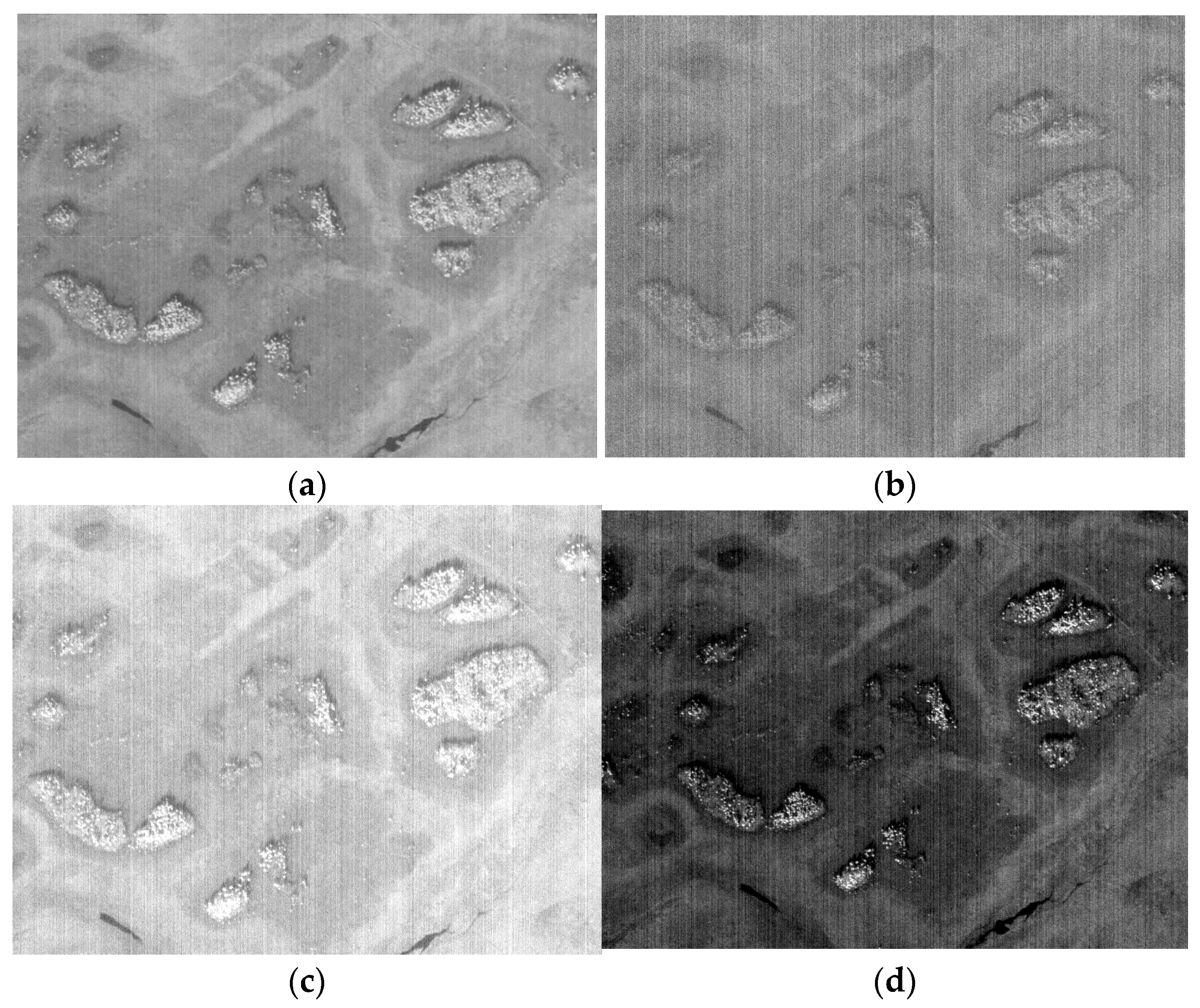
The raw Bayer pattern data was reconstructed into three-band data, as shown in Figure 10. The reconstructed three-band raw data more visually and clearly demonstrates the inconsistent radiometric response between the detectors within a single band, indicating that the reconstructed virtual linear push-broom sensor has the same characteristics as the linear push-broom remote sensing sensors.
The method described in Section 2.3 was used to solve the non-linear calibration parameter for each imaging detector in the RGB band based on the reconstructed sample data. The calibration parameters characterize the mapping between the raw DNs and calibrated DNs for each detector over the quantization range (Figure 11a). The mapping relationship characterizes the radiometric response of a single detector at specific incident radiances and the inconsistency of the radiometric response of different detectors at the same incident radiance. Figure 11b shows the radiometric response curves of each detector at low, medium, and high DNs, indicating that there is a serious non-linear radiometric response at the edges of the CMOS (shown as circles in the figure), while the radiometric response is relatively stable at non-edges. This inconsistency in the radiometric response model between separate imaging detectors indicates that there is some instability in the on-orbit radiometric response of the OVS sensor, which is a major factor affecting the calibration accuracy and poses a challenge for radiometric calibration.
3.2. Visual Assessments
The three-band images reconstructed from the Bayer pattern data were corrected using the relative radiometric calibration parameters. Comparing Figure 12 to Figure 10b–d, the relative corrected three-band images have no streaking or banding noise and no residual streaking, indicating that the detector radiometric response error of the Bayer pattern was calibrated.
To better verify the radiometric correction effect, the original Bayer pattern images before and after the radiometric correction were subjected to Bayer interpolation to obtain RGB color images. The Bayer interpolation algorithm used a fast method of Bayer color reconstruction with a multi-orientation description proposed in the literature [20,21]. Then, the interpolated color images were used to compare and analyze the validity of the radiometric calibration parameters because the human eye is more sensitive to color images. The raw Bayer pattern images of uniform ocean, cloud, and urban areas are shown in Figure 13a,d,g, respectively, with the problem of radiometric response streaks between detectors. Figure 13b,e,h show that the difference in radiometric response between the detectors of the Bayer pattern is enhanced by Bayer interpolation, and that image streaking is evident. This indicates that the Bayer interpolation algorithm enhances the radiometric response error between the detectors of the Bayer pattern and reduces the quality of the image, while the color relationship between the RGB bands is misaligned. The Bayer imaging data were radiometrically corrected and then Bayer interpolated, as shown in Figure 13c,f,i, where image stripes are completely absent, while image texture information is enhanced, color relationships are corrected, and the images are visually good. These characteristics indicate that the radiometric response errors between the original Bayer detectors were well corrected.
The magnified detail comparison of the original Bayer pattern data, the uncorrected interpolated image, and the relative radiometric corrected interpolated image show that the Bayer interpolation without relative radiometric correction lost image details, which prevented it from recovering the true color relationship between the bands (Figure 14b). Figure 14c shows that after relative radiometric calibration and Bayer interpolation, the true color and detailed texture information of the features were fully recovered. The results show that Bayer interpolation was greatly affected by the radiometric response error of the Bayer detectors, and the relative radiometric calibration is an essential step before Bayer interpolation for Bayer pattern type remote sensing sensors.
3.3. Accuracy Assessments
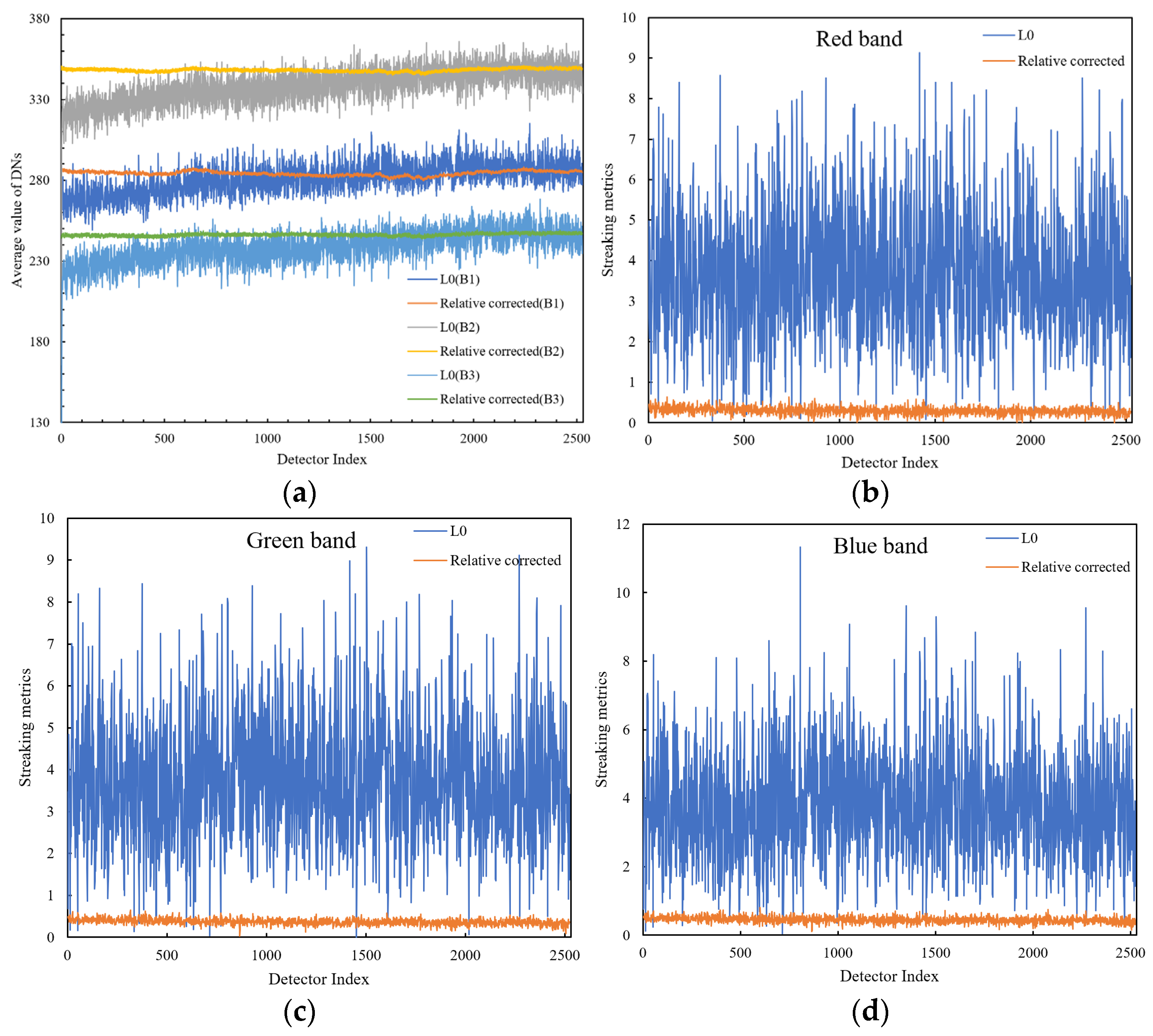
For the quantitative assessment, the residual error in the high-frequency radiometric response between adjacent detectors and the residual error in the low-frequency response between all detectors in the full field of view of the sensor are measured in terms of both the streaking metrics and the root-mean-square for the column mean of the images. In the ocean uniform scene, there is a jump in the mean value of the adjacent columns of the raw image (Figure 15a) and the value of the streaking metrics is much greater than 1% (Figure 15b–d), reaching around 9%. This indicates that there is a greater high frequency radiometric response error for each adjacent detector of the Bayer sensor, while the radiometric response of the left detectors in the field of view is systematically lower than that of the right detectors (Figure 15a). There is also a low frequency radiometric response error in all detectors; however, after radiometric correction, both high- and low-frequency radiometric response errors were eliminated, but the mean values of the images in each band remained unchanged and the spectral characteristics of the features were maintained, which indicates that the radiometric quality of the three-band images was improved (Figure 15) and that the method in this study can calibrate Bayer pattern sensors and eliminate their various low- and high-frequency radiometric response errors.
Furthermore, the specific indexes of a dozen regional radiometric correction images under the various previously mentioned incident radiances were calculated, as shown in Table 2. The accuracy of the relative radiation calibration of three-band the OVS is better than 0.80%, 0.71%, and 0.54% for the red, green, and blue bands, respectively, meeting the requirement of obtaining a relative radiation calibration accuracy better than 3%.
Although the relative radiation correction accuracy for both high and low frequencies of the OVS satellite is better than 1%, there is a tendency for the radiometric correction accuracy to deteriorate for each band at varying DNs. Figure 16 shows that the correction accuracy for low and medium incident DNs was better than that for high DNs and that the relative radiation correction accuracy became progressively worse as the DN increases. This result shows that although the calibration samples are large, the medium DN samples account for the majority of DNs and high DN samples are relatively limited. This results in a lack of accuracy in the expression of the relative radiometric response model relationships between the high DNs, which is a limitation of the statistical calibration method and requires attention in the on-orbit relative radiometric calibration.
4. Discussion
The conversion of a Bayer pattern into a virtual linear array push-broom sensor is the first step in calibration. Moreover, accurately tracking the position relationship of each Bayer pattern before and after the Bayer pattern reconstruction is key to building a calibration sample for each detector. A method using linecounters as the correlation was designed to resolve this issue; however, the solution of the calibration parameters relies on statistical calibration theory, and thus the method has the limitations of statistical calibration methods. The accumulation of a large number of samples, the time-consuming nature of querying statistical samples, the large in-orbit calibration effort, and the low timeliness of the method [19] are among its major limitations. The calibration accuracy is also affected by the sample distribution and the large fluctuations in different brightness ranges [22]. An excessively large single calibration sample results in difficulty in calibrating the complex non-linear radiometric response, an inability to calibrate the full dynamic range radiometric response of the load, or even a failure in calibration. Therefore, on-orbit calibration samples should be selected to cover as many typical features as possible (such as oceans, cities, clouds, and snow), and the number of samples for the various types of features should be as equal as possible. Additionally, the samples should attempt to cover the dynamic range of the sensor to avoid or reduce the influence of the sample distribution on the calibration results.
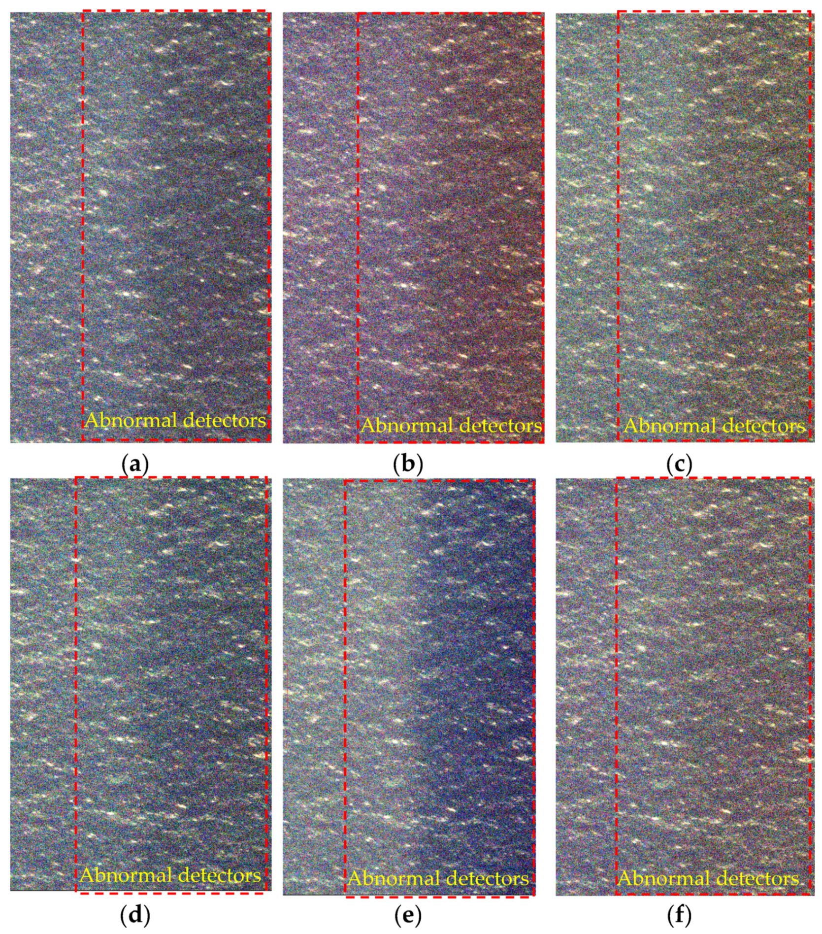
For the OVS satellite, the calibration process identified an occasional anomalous radiometric response issue with some of its CMOS detector edge detectors (Figure 17) with approximately 380 detectors at the CMOS5 edge with an anomalous radiometric response from October to November 2019. The effect of such short periods of large differential radiometric response on on-orbit radiometric calibrations can be fatal, directly causing calibration failure. Anomalous data must be removed from the calibration sample during the orbital radiometric calibration to exclude the partial failure of the calibration coefficients due to sample anomalies; however, this problem needs to be reported to the satellite manufacturer to investigate the fundamental cause of the anomalous radiometric response of the OVS sensor and reduce the difficulty of radiometric calibration. Preliminary analyses of possible causes include the following: the abnormal radiometric response of the camera due to a single particle event, which is automatically recovered after a camera restart; “subtle” differences in the bonding of the filter and the CMOS itself, which causes changes in the light transmission rate; and a camera designed to use the fixed pattern noise (FPN) parameter by default, which may cause abnormal radiometric response if there is a problem with the FPN setting. These shortcomings will be circumvented in subsequent satellite designs.
5. Conclusions
The Zhuhai-1 video satellite plane array Bayer pattern sensor provides two imaging modes for one satellite, which expands the application capability of a single satellite but also brings up new problems for radiometric calibration. This study developed an on-orbit relative radiometric calibration method for the OVS satellite with a Bayer pattern push-broom imaging mode. The novel aspects of this study include:
- (1)
- reconstructing the order of each detector of the Bayer pattern sensor and converting it into a virtual linear array sensor to separate the RGB three-band components from the Bayer pattern; and
- (2)
- designing a positioning method linked by “linecounters” to detect the specific position of each detector of each Bayer pattern.
The visual and quantitative assessment of the calibration and correction results revealed the superior performance of the method at reducing image stripes and preserving image details. Furthermore, this study also provides an effective method for the on-orbit radiometric calibration of Bayer pattern sensors and meaningful lessons for the radiometric calibration of similar remote sensing satellites. The Bayer interpolation algorithm is greatly affected by the radiometric response error of the Bayer detectors. Therefore, the relative radiometric calibration method has a pronounced impact on the Bayer interpolation and must be performed for Bayer pattern type remote sensing sensors.
From the calibration results, the on-orbit relative radiation calibration accuracy of the OVS was better than 1%, meeting the technical index requirements. The image streaks and strip noise were effectively removed after calibration, and the image radiation quality was greatly improved; however, there were occasional radiation response anomalies in the single CMOS edge detectors of the OVS, which increased the uncertainty of the on-orbit radiation calibration and the subsequent application of the image.
Author Contributions
Conceptualization, L.L. and Y.J.; methodology, L.L.; software, Z.L. and Z.W.; validation, X.S. and J.W.; formal analysis, L.L.; investigation, Z.L.; resources, Z.W.; data curation, J.W.; L.L. wrote the paper; and all authors edited the paper. All authors have read and agreed to the published version of the manuscript.
Funding
This research was funded by the National Natural Science Foundation of China, grant number 41971412, 42171341.
Data Availability Statement
Restrictions apply to the availability of these data.
Acknowledgments
We thank the research team at Orbita for providing the OHS images. Furthermore, we would like to thank the reviewers for their helpful comments.
Conflicts of Interest
The authors declare no conflict of interest.
References
- Li, L.; Jiang, L.; Zhang, J.; Wang, S.; Chen, F. A complete YOLO-based ship detection method for thermal infrared remote sensing images under complex backgrounds. Remote Sens. 2022, 14, 1534. [Google Scholar] [CrossRef]
- Teillet, P.M. Image correction for radiometric effects in remote sensing. Int. J. Remote Sens. 1986, 7, 1637–1651. [Google Scholar] [CrossRef]
- Moghimi, A.; Celik, T.; Mohammadzadeh, A. Tensor-based keypoint detection and switching regression model for relative radiometric normalization of bitemporal multispectral images. Int. J. Remote Sens. 2022, 43, 3927–3956. [Google Scholar] [CrossRef]
- Blanchet, G.; Lebegue, L.; Fourest, S.; Latry, C.; Porez-Nadal, F.; Lacherade, S.; Thiebaut, C. Pleiades-HR innovative techniques for radiometric image quality commissioning. In Proceedings of the ISPRS—International Archives of the Photogrammetry, Remote Sensing and Spatial Information Sciences, Melbourne, Australia, 25 August–1 September 2012; Volume XXXIX-B1; pp. 513–518. [Google Scholar]
- Pesta, F.; Bhatta, S.; Helder, D.; Mishra, N. Radiometric non-uniformity characterization and correction of Landsat 8 OLI using earth imagery-based techniques. Remote Sens. 2014, 7, 430–446. [Google Scholar] [CrossRef] [Green Version]
- Kabir, S.; Leigh, L.; Helder, D. Vicarious methodologies to assess and improve the quality of the optical remote sensing images: A critical review. Remote Sens. 2020, 12, 4029. [Google Scholar] [CrossRef]
- Murthy, K.; Shearn, M.; Smiley, B.D.; Chau, A.H.; Levine, J.; Robinson, M.D. SkySat-1: Very high-resolution imagery from a small satellite. In Proceedings of the Sensors, Systems, and Next-Generation Satellites XVIII, Amsterdam, The Netherlands, 22–25 September 2014; Volume 9241, pp. 92411E-1–92411E-12. [Google Scholar]
- Zhang, G.; Li, L.; Jiang, Y.; Shen, X.; Li, D. On-orbit relative radiometric calibration of the night-time sensor of the LuoJia1-01 satellite. Sensors 2018, 18, 4225. [Google Scholar] [CrossRef] [PubMed] [Green Version]
- Zhang, G.; Li, L.T.; Jiang, Y.H.; Shi, X.T. On-orbit relative radiometric calibration of optical video satellites without uniform calibration sites. Int. J. Remote Sens. 2019, 40, 5454–5474. [Google Scholar] [CrossRef]
- Pascal, V.; Lebegue, L.; Meygret, A.; Laubies, M.; Hourcastagnou, J.; Hillairet, E. SPOT5 first in-flight radiometric image quality results. In Proceedings of the Sensors, Systems, and Next-Generation Satellites VI, Crete, Greece, 23–27 September 2002; Volume 4881, pp. 200–211. [Google Scholar]
- Pagnutti, M.; Ryan, R.E.; Kelly, M.; Holekamp, K.; Zanoni, V.; Thome, K.; Schiller, S. Radiometric characterization of IKONOS multispectral imagery. Remote Sens. Environ. 2003, 88, 53–68. [Google Scholar] [CrossRef] [Green Version]
- Anderson, C.; Helder, D.L.; Jeno, D. Statistical relative gain calculation for Landsat 8. In Proceedings of the Conference on Earth Observing Systems XXII, San Diego, CA, USA, August 10 June 2017. [Google Scholar]
- WEGENER, M. Destriping multiple sensor imagery by improved histogram matching. Int. J. Remote Sens. 1990, 11, 859–879. [Google Scholar] [CrossRef]
- Henderson, B.G.; Krauseb, K.S. Relative radiometric correction of QuickBird imagery using the side-slither technique on orbit. In Proceedings of the Earth Observing Systems IX, Denver, CO, USA, 4–6 August 2004; SPIE: Paris, France; Volume 5542, pp. 426–436. [Google Scholar] [CrossRef]
- Gerace, A.; Schott, J.; Gartley, M.; Montanaro, M. An analysis of the side slither on-orbit calibration technique using the DIRSIG model. Remote Sens. 2014, 6, 10523–10545. [Google Scholar] [CrossRef] [Green Version]
- Begeman, C.; Helder, D.; Leigh, L.; Pinkert, C. Relative radiometric correction of pushbroom satellites using the yaw maneuver. Remote Sens. 2022, 14, 2820. [Google Scholar] [CrossRef]
- Zhang, G.; Li, L. A study on relative radiometric calibration without calibration field for YG-25. Acta Geod. Cartogr. Sin. 2017, 46, 1009–1016. [Google Scholar]
- Li, L.; Zhang, G.; Jiang, Y.; Shen, X. An Improved On-Orbit Relative Radiometric Calibration Method for Agile High-Resolution Optical Remote-Sensing Satellites with Sensor Geometric Distortion. IEEE Trans. Geosci. Remote Sens. 2022, 60, 1–15. [Google Scholar] [CrossRef]
- Angal, A.; Helder, D. Advanced Land Imager Relative Gain characterization and Correction. In Proceedings of the Pecora 16—Global Priorities in Land Remote Sensing 2005, Sioux Falls, SD, USA, 23–27 October 2005. [Google Scholar]
- Chung, K.H.; Chan, Y.H. An edge-directed demosaicing algorithm based on integrated gradient. In Proceedings of the 2010 IEEE International Conference on Multimedia and Expo, Singapore, 19–23 July 2010; pp. 388–393. [Google Scholar]
- Pekkucuksen, I.; Altunbasak, Y. Multiscale gradients-based color filter array interpolation. IEEE Trans. Image Process. 2013, 22, 157–165. [Google Scholar] [CrossRef] [PubMed]
- Shrestha, A.K.; Helder, D. Relative gain characterization and correction for pushbroom sensors based on lifetime image statistics. In Proceedings of the Civil Commercial Imagery Evaluation Workshop 2010, Fairfax, VA, USA, 16–18 March 2010. [Google Scholar]
Figure 1.
CMOS arrangement of the focal plane of the OVS satellite (a), “GBRG” Bayer pattern (b), and “GRBG” Bayer pattern (c).
Figure 1.
CMOS arrangement of the focal plane of the OVS satellite (a), “GBRG” Bayer pattern (b), and “GRBG” Bayer pattern (c).

Figure 2.
Workflow of Bayer color reconstruction (a) and a Bayer interpolation example image (b).

Figure 3.
Schematic of Bayer sensor staring (a) and push-broom imaging (b).

Figure 4.
Schematic of multi-level TDI in (a) a linear array push-broom sensor and (b) a Bayer pattern push-broom sensor.
Figure 4.
Schematic of multi-level TDI in (a) a linear array push-broom sensor and (b) a Bayer pattern push-broom sensor.

Figure 5.
Uniform ocean zone images captured from an OVS Bayer sensor: (a) raw Bayer data, (b) color reconstructed image without relative radiometric calibration, and (c) color reconstructed image after relative radiometric calibration.
Figure 5.
Uniform ocean zone images captured from an OVS Bayer sensor: (a) raw Bayer data, (b) color reconstructed image without relative radiometric calibration, and (c) color reconstructed image after relative radiometric calibration.

Figure 6.
Schematic of Bayer pattern conversion at a single integration.

Figure 7.
Schematic of Bayer pattern changes caused by a row data loss (a) from a GBRG Bayer pattern to (b) a RGGB Bayer pattern in lines 3–4.
Figure 7.
Schematic of Bayer pattern changes caused by a row data loss (a) from a GBRG Bayer pattern to (b) a RGGB Bayer pattern in lines 3–4.

Figure 8.
Bayer pattern data with a linecounter.

Figure 9.
Calibration and validation zone data.

Figure 10.
Bayer pattern data (a); conversion to push-broom data, including the red band data (b); green band data (c); and blue band data (d).
Figure 10.
Bayer pattern data (a); conversion to push-broom data, including the red band data (b); green band data (c); and blue band data (d).

Figure 11.
Relative radiometric calibration parameters of OVS mapping between the raw digital numbers (DNs) and the calibrated DNs (a), and radiometric response curves of various detectors under low, medium, and high DNs (b).
Figure 11.
Relative radiometric calibration parameters of OVS mapping between the raw digital numbers (DNs) and the calibrated DNs (a), and radiometric response curves of various detectors under low, medium, and high DNs (b).

Figure 12.
The relative corrected reconstructed Bayer data, including red band data (a), green band data (b), and blue band data (c).
Figure 12.
The relative corrected reconstructed Bayer data, including red band data (a), green band data (b), and blue band data (c).

Figure 13.
Relative corrected images for various feature types of ocean (a–c), clouds (d–f), and urban areas (g–i): raw Bayer pattern images (a,d,g); uncalibrated Bayer interpolation images (b,e,h); and calibrated Bayer interpolation images (c,f,i).
Figure 13.
Relative corrected images for various feature types of ocean (a–c), clouds (d–f), and urban areas (g–i): raw Bayer pattern images (a,d,g); uncalibrated Bayer interpolation images (b,e,h); and calibrated Bayer interpolation images (c,f,i).

Figure 14.
Comparison of a specific Bayer image enlarged four times: (a) raw Bayer data, (b) uncalibrated Bayer interpolation data, and (c) calibrated Bayer interpolation data.
Figure 14.
Comparison of a specific Bayer image enlarged four times: (a) raw Bayer data, (b) uncalibrated Bayer interpolation data, and (c) calibrated Bayer interpolation data.

Figure 15.
Distribution of column means of level zero image (a) and RGB band streaking metrics (b–d) before and after relative correction.
Figure 15.
Distribution of column means of level zero image (a) and RGB band streaking metrics (b–d) before and after relative correction.

Figure 16.
Distribution of image radiometric correction accuracy under various DNs.

Figure 17.
Anomalous changes in the radiometric response of CMOS edge detectors of the OVS at specific times during calibration of the 2019 data: (a) 26 October; (b) 28 October; (c) 29 October; (d) 30 October; (e) 1 November; and (f) 2 November.
Figure 17.
Anomalous changes in the radiometric response of CMOS edge detectors of the OVS at specific times during calibration of the 2019 data: (a) 26 October; (b) 28 October; (c) 29 October; (d) 30 October; (e) 1 November; and (f) 2 November.


Table 1.
Detailed information for the OVS sensor.
| Parameter | Value |
|---|---|
| Ground swath | 22.5 km @ 500 km |
| Imaging mode | Staring video mode: frame rate: 10–25 fps Push-broom mode |
| Resolution | 0.9 m |
| Quantization bits | Video mode: 8 bits Push-broom mode: 10 bits |
| Color | Bayer pattern |
| Modulation Transfer Function | ≥0.12 @ Nyquist frequency |
| Signal To Noise Ratio | ≥35 dB (Sun elevation angle ≥ 50°) |
Table 2.
Accuracy of the OVS satellite relative radiometric calibration.
| CMOS | Zone | Band | Average DNs | Streaking Metrics (%) | RMS (%) |
|---|---|---|---|---|---|
| 1 | 1 | R | 174.464505 | 0.252942 | 0.553052 |
| G | 303.027251 | 0.128574 | 0.389035 | ||
| B | 299.120944 | 0.101004 | 0.286782 | ||
| 2 | R | 145.834542 | 0.602074 | 0.689595 | |
| G | 278.809108 | 0.434780 | 0.380873 | ||
| B | 280.663032 | 0.358834 | 0.377148 | ||
| 3 | R | 187.183937 | 0.834730 | 0.602284 | |
| G | 330.415927 | 0.708178 | 0.472996 | ||
| B | 322.815496 | 0.643862 | 0.382063 | ||
| 4 | R | 633.844315 | 0.505590 | 1.452498 | |
| G | 885.569805 | 0.469941 | 1.384834 | ||
| B | 689.440504 | 0.438069 | 0.987072 | ||
| 2 | 1 | R | 213.339061 | 0.391711 | 0.654857 |
| G | 331.792004 | 0.289577 | 0.598556 | ||
| B | 313.929878 | 0.224774 | 0.529018 | ||
| 2 | R | 183.932816 | 0.818849 | 1.050736 | |
| G | 306.118564 | 0.706289 | 0.998101 | ||
| B | 298.570655 | 0.656120 | 0.635410 | ||
| 3 | R | 210.372869 | 0.212614 | 0.598503 | |
| G | 334.387692 | 0.315220 | 0.538775 | ||
| B | 318.118987 | 0.379993 | 0.545816 | ||
| 4 | R | 677.060288 | 0.188683 | 0.637184 | |
| G | 918.258576 | 0.158117 | 1.107705 | ||
| B | 706.071616 | 0.130670 | 0.643381 | ||
| 3 | 1 | R | 167.416066 | 0.234464 | 0.402989 |
| G | 301.497830 | 0.108619 | 0.220347 | ||
| B | 301.903464 | 0.093085 | 0.289550 | ||
| 2 | R | 126.881600 | 0.549097 | 0.769455 | |
| G | 254.414065 | 0.357859 | 0.607761 | ||
| B | 272.225351 | 0.286836 | 0.363299 | ||
| 3 | R | 623.796314 | 0.814639 | 1.237399 | |
| G | 882.974602 | 0.780348 | 1.039002 | ||
| B | 694.270148 | 0.748270 | 0.548426 | ||
| 4 | 1 | R | 210.705489 | 0.437302 | 0.733809 |
| G | 327.850046 | 0.337556 | 0.424513 | ||
| B | 301.488013 | 0.273422 | 0.451469 | ||
| 2 | R | 169.106208 | 0.420492 | 0.866250 | |
| G | 282.933319 | 0.297154 | 0.726361 | ||
| B | 273.462593 | 0.230403 | 0.564223 | ||
| 3 | R | 194.781064 | 0.151181 | 0.828773 | |
| G | 314.900084 | 0.073915 | 0.573989 | ||
| B | 296.537163 | 0.091034 | 0.663551 | ||
| 4 | R | 678.343272 | 0.188817 | 0.616931 | |
| G | 919.031208 | 0.159909 | 0.740941 | ||
| B | 681.249269 | 0.131942 | 0.742365 | ||
| 5 | 1 | R | 234.104145 | 0.098038 | 0.885455 |
| G | 386.938663 | 0.043580 | 0.674836 | ||
| B | 381.137859 | 0.080850 | 0.595346 | ||
| 2 | R | 179.405221 | 0.160321 | 0.135142 | |
| G | 319.111673 | 0.037737 | 0.185095 | ||
| B | 333.812995 | 0.036985 | 0.176527 | ||
| 3 | R | 212.526180 | 0.542912 | 0.638558 | |
| G | 364.433856 | 0.434148 | 0.476657 | ||
| B | 372.303330 | 0.381670 | 0.367203 |
Disclaimer/Publisher’s Note: The statements, opinions and data contained in all publications are solely those of the individual author(s) and contributor(s) and not of MDPI and/or the editor(s). MDPI and/or the editor(s) disclaim responsibility for any injury to people or property resulting from any ideas, methods, instructions or products referred to in the content. |
© 2023 by the authors. Licensee MDPI, Basel, Switzerland. This article is an open access article distributed under the terms and conditions of the Creative Commons Attribution (CC BY) license (https://creativecommons.org/licenses/by/4.0/).
Share and Cite
MDPI and ACS Style
Li, L.; Li, Z.; Wang, Z.; Jiang, Y.; Shen, X.; Wu, J. On-Orbit Relative Radiometric Calibration of the Bayer Pattern Push-Broom Sensor for Zhuhai-1 Video Satellites. Remote Sens. 2023, 15, 377. https://doi.org/10.3390/rs15020377
AMA Style
Li L, Li Z, Wang Z, Jiang Y, Shen X, Wu J. On-Orbit Relative Radiometric Calibration of the Bayer Pattern Push-Broom Sensor for Zhuhai-1 Video Satellites. Remote Sensing. 2023; 15(2):377. https://doi.org/10.3390/rs15020377
Chicago/Turabian StyleLi, Litao, Zhen Li, Zhixin Wang, Yonghua Jiang, Xin Shen, and Jiaqi Wu. 2023. "On-Orbit Relative Radiometric Calibration of the Bayer Pattern Push-Broom Sensor for Zhuhai-1 Video Satellites" Remote Sensing 15, no. 2: 377. https://doi.org/10.3390/rs15020377
Note that from the first issue of 2016, this journal uses article numbers instead of page numbers. See further details here.