
2D Phase-Based RFID Localization for On-Site Landslide Monitoring


1
Université Grenoble Alpes, Université Savoie Mont Blanc, CNRS, IRD, Université Gustave Eiffel, ISTerre, 38000 Grenoble, France
2
Géolithe, 38920 Crolles, France
*
Author to whom correspondence should be addressed.
Remote Sens. 2022, 14(15), 3577; https://doi.org/10.3390/rs14153577
Submission received: 23 May 2022
/
Revised: 20 July 2022
/
Accepted: 22 July 2022
/
Published: 26 July 2022
(This article belongs to the Special Issue Remote Sensing Techniques for Landslides Studies and Their Hazards Assessment)
Abstract
:Passive radio-frequency identification (RFID) was recently used to monitor landslide displacement at a high spatio-temporal resolution but only measured 1D displacement. This study demonstrates the tracking of 2D displacements, using an array of antennas connected to an RFID interrogator. Ten tags were deployed on a landslide for 12 months and 2D relative localization was performed using a phase-of-arrival approach. A period of landslide activity was monitored through RFID and displacements were confirmed by reference measurements. The tags showed displacements of up to 1.2 m over the monitored period. The centimeter-scale accuracy of the technique was confirmed experimentally and theoretically for horizontal localization by developing a measurement model that included antenna and tag positions, as well as multipath interference. This study confirms that 2D landslide displacement tracking with RFID is feasible at relatively low instrumental and maintenance cost.
1. Introduction
Ground deformation monitoring with high resolution both in space and time remains a challenge due to the high cost of existing solutions, and to environmental limitations, such as meteorological phenomena, rough terrain or dense vegetation. Amongst several remote sensing methods [1,2], surface monitoring of large landslides can be typically performed through interferometric synthetic aperture radar (InSAR), either by space-borne measurements [3,4] or using ground-based stations [5,6,7,8,9]. Despite the high space resolution of these methods, the station cost remains high and the time resolution can be multiple days in the case of satellite remote sensing. More localized techniques, such as GPS [10,11,12,13] and radiofrequency-transponders [14,15], show higher time resolution, but also require on-board power sources which greatly increase initial cost and maintenance.
In this context, radio-rrequency identification (RFID) has shown increasing potential for earth science applications [16,17]. Amongst other applications, it is foreseen as a promising alternative for landslide and civil engineering structure deformation monitoring [18] due to its low cost relative to other solutions, and because it works under rain, snow and vegetation cover conditions [19,20]. It can thus be used as a tool for landslide early-warning [21], forecasting or long-term monitoring [22]. A wide range of solutions exist for tag localization using RFID [23,24], with various possibilities both in measured quantity and in terms of the measuring scheme.
The quantities most used for localization are the received signal strength and the back-scattered phase of arrival. Signal-strength-based methods have been widely used for tag localization [25,26,27,28,29,29]. However, phase-based methods have shown better precision and reliability in recent years [30,31,32], primarily because they are less sensitive to environmental variations and because the phase of the signal varies more rapidly with distance than the received signal strength.
Phase-based localization is divided into multiple schemes, which are extensively presented elsewhere [33,34,35,36]. These schemes generally rely on either multistatic stationary antennas and different carrier frequencies [30,37,38], or on a moving antenna with a known trajectory (e.g., the synthetic aperture radar technique) [39,40,41,42,43]. This paper focuses on a monostatic multi-antenna time-domain phase difference (TD-PD)-inspired scheme, as TD-PD has shown the best results for measuring relative displacements outdoors [18], with a precision of about 1 cm over long time periods for 1D displacement tracking. To date, RFID systems deployed to monitor moving ground only provide one-dimensional distance information and are subject to phase unwrapping issues that could be solved by using multiple antennas. In this article, we test the stationary configuration for 2D RFID tag localization using a set of four antennas in a TD-PD relative localization approach, and also discuss 3D localization perspectives. To the best of our knowledge, this is the first attempt at 2D-localization of RFID tags in an outdoor scenario, using a monostatic, monofrequency multi-antenna setup.
In the following section, we present the instrumentation of the experimental site and the methodology for data acquisition and processing. Section 4 provides theoretical background and experimental validation of the RFID measurement error in order to decide on ideal antenna positioning by optimizing the localization accuracy and phase ambiguity. Section 5 reports on an example of 12 months of surface deformation monitoring on the slow-moving Harmalière landslide.
2. Instrumentation and Methods
2.1. Experimental Site: Harmalière Landslide
The Harmalière landslide (Sinard, Isère, France) is located in the Trièves area about 50 km south of Grenoble in the western Prealps (see Figure 1). Trièves appears as a sedimentary plateau eroded by the Drac river; the plateau is formed by Quaternary varved clays and alluvial materials deposited in a glacially dammed lake during the Würm period [44]. Quaternary sediments also include silts, sometimes with a morainic cover, and rest on either interglacial Riss-–Würm period glaciofluvial materials (gravels and sands) or on the underlying Jurassic carbonate bedrock. The thickness of the clay deposits can vary from 0 to a maximum of 200 m [45]. The landslide is southeast oriented, 400 m wide at the top, narrowing to 150 m at the toe. It develops from an altitude of 735 m (asl), down to the Monteynard Lake (480 m), over a distance of about 1.5 km. It was abruptly activated in 1981 and has remained active ever since, with new peaks of activity in 2016 and 2017 [46]. The slow moving landslide shows regressive behaviour, the headscarp retreating at an average velocity of 1 m/year, with very strong variations from year-to-year (including almost a decade of rest). The central body of the landslide is moving at velocities ranging from cm/year to m/year, with possible dramatic acceleration phases (m/day). A variety of research subjects are currently investigated in connection with it [46,47].
2.2. RFID Instrumentation and Localization
2.2.1. RFID Instrumentation
In February 2020, a section of the landslide was equipped with an RFID system consisting of 32 battery-assisted passive tags and an acquisition station located near the landslide scar (see Figure 1). These tags can last about a decade without maintenance or replacement in the present real-time monitoring scenario. The station includes four antennas, an interrogator (Impinj SR420), a micro-computer (RPI-3B), and a modem to send the data automatically to a remote server, as described by (patent pending FR-17/53739). It is powered by a photovoltaic module and a wind turbine. The station collects RFID data for 3 min every 20 min from every tag and every antenna. The data includes the phase of arrival (termed here "phase") measured at 865.7 Hz, the received signal strength indication and the tag temperature. The tags were placed in pairs on fiber glass stakes 50 cm and 1 m above ground. They were spread out within the antennas reading range in a zone approximately 30 m × 30 m wide (see Figure 1), in such a way as to maximize the line-of-sight readability of each tag by multiple antennas. To validate the RFID localization calculations, the position of the tags was measured with a LEICA TCR805 tacheometer and a handheld target (estimated precision 4 cm), approximately once every month.
2.2.2. RFID Localization Scheme
TD-PD is a relative ranging technique based on phase variation between two measurements at different points in time. is related to the radial distance variation between the tag and reader antenna, by the following equation:
where f is the frequency of the electromagnetic wave (see values above) and c is the speed of light in the propagation medium. It is important to note that Equation (1) is only valid for displacements smaller than cm between two phase measurements because of phase ambiguity. In the present case, this condition is generally fulfilled as the incremental displacements are small compared to the wavelength (usually less than 1 cm between two successive acquisitions). Moreover, a series of phase measurements can generally be unwrapped using well-defined algorithms. In this case, Equation (1) is valid for any unwrapped phase variation.
Section 3 presents a multidimensional localization scheme based on TD-PD.
3. Theoretical Model
In this section, we derive a mathematical model for phase-based RFID localization to compute the localization error of our real experiment. The main goal of this derivation is to study the origins of the localization uncertainty, mainly with respect to the system geometry and the physical measurement process.
From now on, we will consider that all phase measurements are unwrapped, and that Equation (1) is valid for all phase variations. Most presented tags were correctly read and no unwrapping error was detected in the monitored period. The specific case of an unwrapping error is examined separately, and does not fall within the scope of the present study.
In the following, index i describes a series of measurements starting at and j describes the antenna indexing.
3.1. Localization Model
3.1.1. One Dimensional TD-PD
The localization method presented in this paper is based on the tag phase shift measured by each antenna at different points in time (TD-PD) [36]. In a homogeneous medium, the phase shift between the initial and the i-th (unwrapped) phase measurement, is directly proportional to the radial displacement between the tag and antenna j (see Equation (1)).
Assuming an initial radial distance , we obtain a series of radial distances from a measured phase series :
where is obtained directly through Equation (1). This localization method is, hence, relative to the initial position, as it does not allow for absolute positioning without further information about the system (e.g., when is not known).
3.1.2. 2D Relative Displacement Approach
Using the measurements of multiple antennas, we can expand this TD-PD method with spatial considerations. For this purpose, we need both the phase measurements and the geometrical coordinates of each antenna. This derivation focuses on the 2D problem; the 3D case will be briefly discussed at the end.
We define the initial distance from the antenna j to the tag:
where are the initial coordinates of the tag and those of the antenna.
Applying Equation (2), we obtain a series of radial displacements from the phase measurements of each antenna. From these radial distance measurements, a multilateration approach [48] can be applied to estimate the most probable position for the tag at the ith position. Amongst various possible methods of multilateration, we use an optimization algorithm that minimizes the following cost function for the i-th measurement:
where are the test point coordinates, is the number of antennas, is the i-th radial distance from antenna j, and is the most probable tag position. The minimization of this cost function was performed using the Trust-region optimization algorithm [49] implemented in the Scipy-optimize Python module.
3.2. Geometrical Localization Sensitivity
In this section, we focus on theoretical considerations regarding the localization sensitivity of the geometrical antenna-tag system to compute the value and direction of a displacement error of the tag with respect to a phase measurement error [19]. For a given antenna position , the absolute phase accumulated on a linear ray path (line of sight, LOS) between the antenna and a point is expressed as follows:
Let us define as the space gradient of the measured phase , also defined as the phase sensitivity kernel, expressed in the spatial dimension as:
For a system consisting of two antennas (A and B) and small phase variations, the relation between the phase variation vector and the true tag displacement can then be approximated by the linear matrix system:
That we can simply rewrite:
Equation (5) holds for any number of phase measurements (thus any number of antennas ), and any number of space dimensions M; in such cases, K will be an matrix. It expresses the direct solution of the phase-based relative localization problem, where K represents the transformation matrix from measured phase space to localization space.
For the sake of simplicity, consider now that , which implies a bijective relationship between phase measurements and tag 2D relative displacement. In this case, the invertibility of the K matrix is almost always possible—the only exceptions are when the point position coincides with that of one antenna, or when it is aligned with the two antennas. We exclude these limit cases that have no significance in our experiments. The above equation can then be reversed and gives the theoretical phase sensitivity of the tag position:
We now consider the linear transformation matrix to which we apply singular value decomposition (SVD). Any real matrix can be decomposed as follows [50]:
In our model, represents the eigenvectors in phase space, the diagonal eigenvalue matrix and U the eigenvectors in localization space.
In this derivation, we assume the same variance for all phase measurements; hence, the covariance matrix is defined as follows:
where is the typical phase standard deviation and is an identity matrix of size . is, thus, a constant diagonal matrix in our model, with typical values of 0.04 rad. This phase standard deviation is both an experimentally computed value and also corresponds to the modeled approximation of Equation (12) (see next Section).
Considering a given phase measurement uncertainty for each antenna, we can plug any phase distribution into the transformation from Equation (7). The shape and orientation of the resulting spatial distribution around tag position (that we will call localization spot) is described by the localization-space covariance matrix . This matrix can be expressed in the following way, depending on as well as the hypothetical covariance of the phase measurement matrix :
Extracting the eigenvalues and eigenvectors of allows for a completely analytical determination of the localization spot properties (especially the direction of highest error) for a given antenna-tag geometry, as shown in Figure 2. With a phase error of 0.04 rad, and at the given tag position, we expect a localization random error of about 1 cm. Note that in the model, any relative increase in phase error will result in the same relative increase in localization error, as the measurement operator is linear.
The calculation presented above can be extended to a three-antenna system for a 3D localization problem, following Equations (1) to (9) with K a matrix. In the case where , the system from Equation (5) is overdetermined, and a least-squares solution has to be found [51,52]. Using the pseudo-inverse of K, Equation (6) then gives:
This new system can be solved and the eigenvectors computed by considering the transformation matrix .
3.3. Phase Error Model: Multipath, Phase Standard Deviation and Radiation Pattern
While the previous section focuses on geometrical localization error, we will now incorporate the impact of real-scenario error sources, e.g., antenna radiation pattern and multipath. The following derivation is based on the work of [20].
3.3.1. Multipath Propagation Model
Multipath interference is a major challenge in RFID-localization and several solutions have been proposed to estimate, reduce or mitigate its effect on measurements [53,54]. To start investigating the multipath, we use a simple two-ray model, assuming that the measured signal is a superposition of the line-of-sight () signal and a signal reflected on the ground (), as shown in Figure 3. The two signals propagate over different path lengths and orientations, which translate in different received power values due to Friis’ law:
where is the power transmitted by the antenna, is the received power along path p, and are the receiver and transmitter gain which depend on the signal orientation angle and the antenna radiation pattern, is the carrier wavelength and is the path propagation distance. We can then define the amplitude gain for the line-of-sight (1) and reflected (2) signals:
where is the reflection coefficient impacting the reflected ray (which depends on ground relative permittivity). The received signal voltage after normalization by the initial emitted voltage can be expressed by the following phasor:
where k is the wave number. The resulting signal arriving on the tag is the sum of the two phasors:
After accounting for tag modulation efficiency [55], and due to the reciprocity of all gain values during the back-scattered propagation, the full signal phasor received by the station antenna is finally expressed as follows:
As a reminder, the squared corresponds to the back-and-forth path of the signal.
3.3.2. Two Types of Phase Error
We define the phase measurement error as the difference between the ideal LOS phase and the full received phase. This error can be divided into two contributions: the phase random deviation and the systematic phase bias , which are both consequences of multipath interference. Let us now consider these two error contributions separately. Previous investigations [18] have shown a direct relationship between antenna received power P(W) and phase random deviation (rad), using the same acquisition configuration (tag, interrogator, and communication protocol):
where c is the light velocity and f the carrier frequency. This empirical relationship reproduces the phase error value of 0.04 rad used in the previous section. The received power greatly depends on propagation distance, but also on multipath interference, which is why is multipath-sensitive. The systematic phase bias is defined as the difference between the ideal LOS phase and the full received phase :
The phase bias obviously depends on multipath behaviour. In phase space, the two error contributions and can be interpreted, respectively, as a scaling and translation operation on an ideal phase measurement distribution. Indeed, represents the width of the measurement error distribution, and the bias represents the center of this distribution; compared to the LOS ideal measurement; the true measurement will thus be translated by and scaled to a width of . Assuming Gaussian behaviour for the measurement process, each antenna j will, hence, present a measurement distribution following a normal law:
These considerations can be applied in the phase-localization scheme presented in the previous section via a multi-antenna phase distribution.
Let us define the scaling matrix S and the translation vector T as follows:
The entries of S originate from Equation (12) and the entries of T from Equation (13). They correspond to the values of phase random error and phase bias measured by each antenna ( = 2 in this simple scenario). Note that the phase random deviation values are different for each antenna for geometrical reasons; each antenna is in a different location, hence, the multipath and radiation patterns do not yield the same error values. The scaling S in phase space allows for a definition of the phase covariance matrix :
can be used in the singular value decomposition to compute the displacement error eigenvectors via the displacement covariance matrix (see Equation (9)). The localization spot dimensions are, hence, fully described by the following covariance matrix in displacement space :
On the other hand, the translation T induced by the phase bias corresponds to a translation in displacement space, obtained by:
Equations (14) and (15) represent our best attempt to model the deviation from an ideal LOS phase measurement, taking into account the various phase measurement errors, and the geometry of the system. Figure 4 presents a 2D schematic view of the measurement distributions from phase space to displacement space. We see that the phase distribution is scaled and translated in phase space, compared to the centered distribution that was set in Equation (8). In displacement space, this gives a specific localization spot with covariance , translated from the true LOS measurement by vector . The specific values of and are discussed in Section 4.2.
4. Harmalière Landslide Monitoring
In this section, we will discuss the specific case of the Harmalière landslide RFID system. After presenting the acquired data, the theoretical model will be applied to the real system geometry, then the localization results will be presented.
4.1. Real Phase Data
Among the 32 tags installed in the field, 10 were read almost continuously by more than two antennas for 12 months (January 2021–February 2022). The rest of the tags yielded partial results that could not be used for 2D localization via the present scheme. Two main factors can explain the lack of readability of some tags, namely, the narrow horizontal directivity of the antennas (+/−30° aperture) and signal attenuation—the furthest tags showed the lowest signal quality. Generally speaking, the tags placed 50 cm above ground showed worse results than those placed 1 m above ground, both in terms of data quality and localization accuracy. This observation corresponds to the above theoretical results (see Section 4.2 and Figure 5c), which tend to show that displacements close to the ground are subject to stronger multipath interference. This study will only show the tags read by at least two antennas during the whole period. The unwrapped phase measured during the January 2021–February 2022 time period is presented in Figure 6 for tag A. The data (70 measurements per day) were averaged over 24 h periods before applying the localization algorithm to mitigate the daily phase variations due to humidity and temperature. The missing values correspond to strong weather events that most likely depleted the battery of the acquisition system, or to hardware failures.
4.2. Application of the Model to a Real Geometry
Before presenting the localization results, we will first apply the previously developed model to the real system geometry. The workflow is presented in Figure 7, showing how the real parameters come together with the geometry and model to compute the localization error mapping.
We have set the model geometry according to Table 1, which corresponds to the Harmalière setup geometry. The number of antennas is now set to . The ground relative permittivity is set according to the literature for dry soils [56,57], and the following results correspond to this dry soil scenario. In the case of a wet soil, we expect the relative permittivity to reach values around 25. In the model, this turned out generally to increase the phase error (and localization error) values by about 30%, which can represent millimeter to centimeter values depending on the context (see Section 4.2.2).
4.2.1. Random Localization Error of the Experimental Field
The previous developments (Equations (14) and (15)) have been applied to the geometry installed in the Harmalière landslide, as shown in Figure 5. A mapping of the random localization error (related to , Equation (12)) is shown in Figure 5a. We see that the lowest error is obtained when facing the antennas, which are oriented eastward. The plot is separated in two main areas, discriminated by the 2 cm random localization error value. This value was chosen because it reflects the target precision in our application.
4.2.2. Systematic Localization Bias of the Experimental Field
The systematic localization bias (related to , Equation (13)) presented in Figure 5b,c is not to be understood as a raw localization error, but as a varying bias when moving in space; the interference between LOS and the reflected signal changes with tag position.
To better understand the effect of the multipath-induced phase bias on 3D displacement measurements, we propose to consider the typical case of a 1 m displacement along a given spatial direction, starting from the position of tag A. The symmetry of our experiment being mainly cylindrical, we consider a cylindrical coordinate system with its central axis in (, ). For this displacement, we compute the localization bias fluctuation, and project it on every space direction (along , , ) to obtain an amplitude value. The displacement length of 1 m was chosen both because it encompasses about one phase bias cycle, and because it corresponds to the actual displacement we measured in the real landslide scenario (see next section).
Table 2 reports the simulated localization bias amplitude in the three space directions, together with real error measurements that were performed on field.
- The direction that produces the least bias variation is a displacement, which corresponds to the quasi rotational symmetry of the system.
- A horizontal displacement along yields a small localization error. This confirms previous studies and demonstrates a centimeter precision for the RFID technique in the horizontal plane [18].
- A vertical displacement along undergoes several strong bias oscillations (Figure 5c). The subsequent localization error is a cumulative effect of both the strong multipath interference and the small vertical aperture of the measurement system.

Table 2.
Direction-dependent localization bias in the 3 directions (cylindrical coordinates), for a typical 1 m displacement. Each column corresponds to a different direction of displacement. Each line represents the localization bias amplitude along a certain direction, during the 1 m displacement. The values in italic correspond to field experiment localization bias measurements.
| Dir. | ||||
|---|---|---|---|---|
| Bias | ||||
| max. bias | <1 cm | <1 cm | 10 cm | |
| (1 cm ) | (20 cm) | |||
| max. bias | 1 cm | 1 cm | 2 cm | |
| (1 cm) | (15 cm) | |||
| max. bias | 1 cm | <1 cm | 70 cm | |
| (5 cm) | (110 cm) | |||
These results tend to show that vertical localization in the current localization scheme cannot be performed with precision. The multipath effect, along with the high system sensitivity in this direction, yield a very high localization bias. This is why we will not present localization results in the following section. This model highlights the importance of the geometrical features of the system, such as antenna position and spacing, tag height and direction of displacement.
4.3. Surface Displacement Monitoring Results
In this section, we present the experimental localization of the tags in the Harmalière landslide. We first focus on the 2D localization of one specific tag (tag A) in Figure 1, then we recapitulate on the whole setup and discuss the results.
4.3.1. 2D Relative Displacement for One Tag
The 2D displacement of tag A, computed from the radial displacements using multilateration and data from the four antennas (see Equation (3)), is shown in Figure 8 against reference tacheometer position measurements. The xOy results are in good agreement with the reference points. Note that, for stable phase periods (for example July 2021), the localization algorithm yields very stable results with a centimeter scale variability, which is in agreement with the theoretical localization error presented in Figure 2. This correspondence between theory and experiment during stable periods is observed for several tags, further validating the measurement error model. Note that Figure 2 does not present any phase bias results, but focuses only on measurement random deviation (dimensions of the localization spot).
4.3.2. 2D Localization for All Tags
Figure 9 shows an overview of the xOy displacement norm measured by the RFID-phase for all available tags during the measurement period. The total displacement is also shown for every tag in Table 3. All RFID localization results fit with reference measurements, notably for displacements greater than 1 m. The steep displacement increase in January 2022 concerning tags 51, 4e and A, was confirmed by tacheometer measurement. This rapid and localized deformation generated cracks and a landslide retrogression of about two meters in this area. A south-east tendency is clearly validated and corresponds to the landslide main direction, as can be seen in the qualitative vector mapping in Figure 10, with various displacement amplitudes depending on tag location. This opens the way to 2D spatio-temporal monitoring of the landslide surface, offering the possibility to better understand the physical mechanisms at the origin of the landslide activation and propagation, and to build new early warning monitoring systems.
4.4. Discussion
In this section we briefly discuss some of the results presented in this paper, as well as future development of the RFID localization system.
4.5. Localization Error and Reference Measurements
In the context in which RFID localization was performed, absolute reference localization at a centimeter level was a complicated task. For practical reasons, reference positions taken via GPS were not sufficiently accurate to be compared to the RFID localization results. This is why tacheometry was used, which is a relative localization method. A landslide is an ever-changing environment, and using absolute references such as trees or antennas involves several sources of error. For this reason, the tacheometer uncertainty given in Table 3 is ±4 cm. As has been described in previous reports [18], RFID phase outdoor localization can outperform the reference measurements.
4.5.1. Discussion on Antenna Position
The above model (Section 4.2) is a tool for optimizing the antenna positions in a given terrain to minimize localization errors originating from both multipath and geometry. We performed calculations for several geometrical cases in a plane xOy geometry, searching for the lowest random deviation in the monitored zone. As a general rule, we conclude that surrounding the field with antennas yields the best accuracy (lowest localization random deviation). For example, if four antennas are spread around the Harmalière field, the horizontal random localization error is expected to reduce to 1 mm.
Such setups are not always possible in real-environment operational situations—the experimental setup obviously has to be designed taking into account the operational constraints and priorities. In cases where a portion of the field is inaccessible, for example, the distance between antennas (system aperture) should be maximized to obtain the lowest random deviation. This guideline has limitations, such as cable length or station cost, hence the final setup will generally be a compromise between precision and station/maintenance cost. Note that other localization methods, such as angle of arrival techniques [54,58] rely on different system geometries and will not lead to the same optimal antenna disposition. The guidelines provided here only apply to a relative displacement scheme; absolute positioning is a different matter which we do not discuss here.
4.5.2. Perspective for Improving Data Availability
In this investigation, the tags that yielded only partial data (i.e., less than two antenna readings, long time periods without data) were not used, although more complex data assimilation techniques could be of use [59,60]. Exploiting both the knowledge of the landslide mechanics and the redundancy of information that the system yields could allow tag monitoring even in partial data scenarios, which are a common issue in outdoor environments. Such techniques will be implemented in future work.
5. Conclusions
We have derived a phase-based 2D localization error theoretical model that allows for error estimation in a scenario of two to four static interrogator antennas, taking into account the specific setup geometry. The model is based on both the sensitivity kernel of the measurement system and a two-ray propagation model (multipath). Under certain conditions, this model confirms the ability to track centimetric ground displacements. The in-plane horizontal measurements demonstrate much better accuracy than the out-of-plane vertical measurements, due to the preferential horizontal antenna distribution, and to ground-reflection multipath interference.
A set of RFID tags was placed on an active landslide and phase measurements were performed over several months to monitor the tags’ displacement. The results show a clear south-east displacement of about 1 m in the horizontal plane over the monitored area. The presented method, inspired by the time-difference phase-difference scheme, has shown very good results for the monitoring of relative displacements in 2D at the centimeter scale. The monitoring of landslides using RFID technology was demonstrated to be a viable solution, with centimeter-scale accuracy over large periods of time. A further step in large scale monitoring could be to deploy a moving antenna (SAR) over greater lengths, and to implement a data assimilation approach to increase data availability.
Author Contributions
Conceptualization, A.C., M.L.B., E.L. and L.B.; Data curation, A.C.; Funding acquisition, M.L.B., E.L. and L.B.; Investigation, A.C.; Methodology, M.L.B., E.L. and L.B.; Supervision, M.L.B., E.L. and L.B.; Validation, A.C., M.L.B., E.L. and L.B.; Writing—original draft, A.C.; Writing—review & editing, M.L.B., E.L. and L.B. All authors have read and agreed to the published version of the manuscript.
Funding
This work was partially funded by the ANR LABCOM GEO3ILAB and by the Region Auvergne Rhone Alpes RISQID project. This work is part of the “Habitability” LABEX coordinated by OSUG. We acknowledge experimental help from B. Vial, M. Langlais, G. Scheiblin, and G. Bièvre from ISTerre.
Conflicts of Interest
The authors declare no conflict of interest.
References
- Scaioni, M.; Longoni, L.; Melillo, V.; Papini, M. Remote sensing for landslide investigations: An overview of recent achievements and perspectives. Remote Sens. 2014, 6, 9600–9652. [Google Scholar] [CrossRef] [Green Version]
- Zhao, C.; Lu, Z. Remote sensing of landslides—A review. Remote Sens. 2018, 10, 279. [Google Scholar] [CrossRef] [Green Version]
- Colesanti, C.; Wasowski, J. Investigating landslides with space-borne Synthetic Aperture Radar (SAR) interferometry. Eng. Geol. 2006, 88, 173–199. [Google Scholar] [CrossRef]
- Strozzi, T.; Farina, P.; Corsini, A.; Ambrosi, C.; Thüring, M.; Zilger, J.; Wiesmann, A.; Wegmüller, U.; Werner, C. Survey and monitoring of landslide displacements by means of L-band satellite SAR interferometry. Landslides 2005, 2, 193–201. [Google Scholar] [CrossRef]
- Wang, Y.; Hong, W.; Zhang, Y.; Lin, Y.; Li, Y.; Bai, Z.; Zhang, Q.; Lv, S.; Liu, H.; Song, Y. Ground-based differential interferometry SAR: A review. IEEE Geosci. Remote Sens. Mag. 2020, 8, 43–70. [Google Scholar] [CrossRef]
- Tarchi, D.; Casagli, N.; Fanti, R.; Leva, D.D.; Luzi, G.; Pasuto, A.; Pieraccini, M.; Silvano, S. Landslide monitoring by using ground-based SAR interferometry: An example of application to the Tessina landslide in Italy. Eng. Geol. 2003, 68, 15–30. [Google Scholar] [CrossRef]
- Monserrat, O.; Crosetto, M.; Luzi, G. A review of ground-based SAR interferometry for deformation measurement. ISPRS J. Photogramm. Remote Sens. 2014, 93, 40–48. [Google Scholar] [CrossRef] [Green Version]
- Helmstetter, A.; Garambois, S. Seismic monitoring of Séchilienne rockslide (French Alps): Analysis of seismic signals and their correlation with rainfalls. J. Geophys. Res. Earth Surf. 2010, 115. [Google Scholar] [CrossRef]
- Aryal, A.; Brooks, B.A.; Reid, M.E.; Bawden, G.W.; Pawlak, G.R. Displacement fields from point cloud data: Application of particle imaging velocimetry to landslide geodesy. J. Geophys. Res. Earth Surf. 2012, 117. [Google Scholar] [CrossRef]
- Benoit, L.; Briole, P.; Martin, O.; Thom, C.; Malet, J.P.; Ulrich, P. Monitoring landslide displacements with the Geocube wireless network of low-cost GPS. Eng. Geol. 2015, 195, 111–121. [Google Scholar] [CrossRef]
- Li, Y.; Huang, J.; Jiang, S.H.; Huang, F.; Chang, Z. A web-based GPS system for displacement monitoring and failure mechanism analysis of reservoir landslide. Sci. Rep. 2017, 7, 17171. [Google Scholar] [CrossRef] [Green Version]
- Šegina, E.; Peternel, T.; Urbančič, T.; Realini, E.; Zupan, M.; Jež, J.; Caldera, S.; Gatti, A.; Tagliaferro, G.; Consoli, A.; et al. Monitoring Surface Displacement of a Deep-Seated Landslide by a Low-Cost and near Real-Time GNSS System. Remote Sens. 2020, 12, 3375. [Google Scholar] [CrossRef]
- Dong, M.; Wu, H.; Hu, H.; Azzam, R.; Zhang, L.; Zheng, Z.; Gong, X. Deformation prediction of unstable slopes based on real-time monitoring and deepar model. Sensors 2020, 21, 14. [Google Scholar] [CrossRef]
- Intrieri, E.; Gigli, G.; Gracchi, T.; Nocentini, M.; Lombardi, L.; Mugnai, F.; Frodella, W.; Bertolini, G.; Carnevale, E.; Favalli, M.; et al. Application of an ultra-wide band sensor-free wireless network for ground monitoring. Eng. Geol. 2018, 238, 1–14. [Google Scholar] [CrossRef]
- Mucchi, L.; Jayousi, S.; Martinelli, A.; Caputo, S.; Intrieri, E.; Gigli, G.; Gracchi, T.; Mugnai, F.; Favalli, M.; Fornaciai, A.; et al. A flexible wireless sensor network based on ultra-wide band technology for ground instability monitoring. Sensors 2018, 18, 2948. [Google Scholar] [CrossRef]
- Schneider, J.M.; Turowski, J.M.; Rickenmann, D.; Hegglin, R.; Arrigo, S.; Mao, L.; Kirchner, J.W. Scaling relationships between bed load volumes, transport distances, and stream power in steep mountain channels. J. Geophys. Res. Earth Surf. 2014, 119, 533–549. [Google Scholar] [CrossRef]
- Breton, M.L.; Liébault, F.; Baillet, L.; Charléty, A.; Larose, E.; Tedjini, S. Dense and longdterm monitoring of Earth surface processes with passive RFID—A review. arXiv 2021, arXiv:2112.11965. [Google Scholar]
- Le Breton, M.; Baillet, L.; Larose, E.; Rey, E.; Benech, P.; Jongmans, D.; Guyoton, F.; Jaboyedoff, M. Passive radio-frequency identification ranging, a dense and weather-robust technique for landslide displacement monitoring. Eng. Geol. 2019, 250, 1–10. [Google Scholar] [CrossRef]
- Le Breton, M.; Baillet, L.; Larose, E.; Rey, E.; Benech, P.; Jongmans, D.; Guyoton, F. Outdoor uhf rfid: Phase stabilization for real-world applications. IEEE J. Radio Freq. Identif. 2017, 1, 279–290. [Google Scholar] [CrossRef]
- Le Breton, M. Suivi Temporel d’un Glissement de Terrain à l’Aide d’Étiquettes RFID Passives, Couplé à l’Observation de Pluviométrie et de Bruit Sismique Ambiant. Ph.D. Thesis, Université Grenoble Alpes (ComUE), Grenoble, France, 2019. [Google Scholar]
- Intrieri, E.; Gigli, G.; Mugnai, F.; Fanti, R.; Casagli, N. Design and implementation of a landslide early warning system. Eng. Geol. 2012, 147, 124–136. [Google Scholar] [CrossRef] [Green Version]
- Intrieri, E.; Carlà, T.; Gigli, G. Forecasting the time of failure of landslides at slope-scale: A literature review. Earth-Sci. Rev. 2019, 193, 333–349. [Google Scholar] [CrossRef]
- Balaji, R.; Malathi, R.; Priya, M.; Kannammal, K. A Comprehensive Nomenclature Of RFID Localization. In Proceedings of the 2020 International Conference on Computer Communication and Informatics (ICCCI), Coimbatore, India, 22–24 January 2020; pp. 1–9. [Google Scholar]
- Miesen, R.; Ebelt, R.; Kirsch, F.; Schäfer, T.; Li, G.; Wang, H.; Vossiek, M. Where is the tag? IEEE Microw. Mag. 2011, 12, S49–S63. [Google Scholar] [CrossRef]
- Ni, L.M.; Liu, Y.; Lau, Y.C.; Patil, A.P. LANDMARC: Indoor location sensing using active RFID. In Proceedings of the 1st IEEE International Conference on Pervasive Computing and Communications, 2003.(PerCom 2003), Fort Worth, TX, USA, 23–26 March 2003; pp. 407–415. [Google Scholar]
- Subedi, S.; Pauls, E.; Zhang, Y.D. Accurate localization and tracking of a passive RFID reader based on RSSI measurements. IEEE J. Radio Freq. Identif. 2017, 1, 144–154. [Google Scholar] [CrossRef]
- Rohmat Rose, N.D.; Low, T.J.; Ahmad, M. 3D trilateration localization using RSSI in indoor environment. Int. J. Adv. Comput. Sci. Appl. 2020, 11, 385–391. [Google Scholar]
- Martinelli, F. A robot localization system combining RSSI and phase shift in UHF-RFID signals. IEEE Trans. Control. Syst. Technol. 2015, 23, 1782–1796. [Google Scholar] [CrossRef]
- Shen, L.; Zhang, Q.; Pang, J.; Xu, H.; Li, P. PRDL: Relative localization method of RFID tags via phase and RSSI based on deep learning. IEEE Access 2019, 7, 20249–20261. [Google Scholar] [CrossRef]
- Scherhäufl, M.; Pichler, M.; Stelzer, A. UHF RFID localization based on evaluation of backscattered tag signals. IEEE Trans. Instrum. Meas. 2015, 64, 2889–2899. [Google Scholar] [CrossRef]
- Wang, Z.; Ye, N.; Malekian, R.; Xiao, F.; Wang, R. TrackT: Accurate tracking of RFID tags with mm-level accuracy using first-order taylor series approximation. Ad Hoc Netw. 2016, 53, 132–144. [Google Scholar] [CrossRef]
- Zhou, C.; Griffin, J.D. Accurate phase-based ranging measurements for backscatter RFID tags. IEEE Antennas Wirel. Propag. Lett. 2012, 11, 152–155. [Google Scholar] [CrossRef]
- Li, C.; Mo, L.; Zhang, D. Review on UHF RFID localization methods. IEEE J. Radio Freq. Identif. 2019, 3, 205–215. [Google Scholar] [CrossRef]
- Huiting, J.; Flisijn, H.; Kokkeler, A.B.; Smit, G.J. Exploiting phase measurements of EPC Gen2 RFID tags. In Proceedings of the 2013 IEEE International Conference on RFID-Technologies and Applications (RFID-TA), Johor Bahru, Malaysia, 4–5 September 2013; pp. 1–6. [Google Scholar]
- Pelka, M.; Bollmeyer, C.; Hellbrück, H. Accurate radio distance estimation by phase measurements with multiple frequencies. In Proceedings of the 2014 International Conference on Indoor Positioning and Indoor Navigation (IPIN), Busan, Korea, 27–30 October 2014; pp. 142–151. [Google Scholar]
- Nikitin, P.V.; Martinez, R.; Ramamurthy, S.; Leland, H.; Spiess, G.; Rao, K. Phase based spatial identification of UHF RFID tags. In Proceedings of the 2010 IEEE International Conference on RFID (IEEE RFID 2010), Orlando, FL, USA, 14–16 April 2010; pp. 102–109. [Google Scholar]
- Povalac, A.; Sebesta, J. Phase difference of arrival distance estimation for RFID tags in frequency domain. In Proceedings of the 2011 IEEE International Conference on RFID-Technologies and Applications, Sitges, Spain, 15–16 September 2011; pp. 188–193. [Google Scholar]
- Scherhäufl, M.; Pichler, M.; Stelzer, A. UHF RFID localization based on phase evaluation of passive tag arrays. IEEE Trans. Instrum. Meas. 2014, 64, 913–922. [Google Scholar] [CrossRef]
- Buffi, A.; Nepa, P.; Cioni, R. SARFID on drone: Drone-based UHF-RFID tag localization. In Proceedings of the 2017 IEEE International Conference on RFID Technology & Application (RFID-TA), Warsaw, Poland, 20–22 September 2017; pp. 40–44. [Google Scholar]
- Buffi, A.; Motroni, A.; Nepa, P.; Tellini, B.; Cioni, R. A SAR-based measurement method for passive-tag positioning with a flying UHF-RFID reader. IEEE Trans. Instrum. Meas. 2018, 68, 845–853. [Google Scholar] [CrossRef]
- Motroni, A.; Nepa, P.; Magnago, V.; Buffi, A.; Tellini, B.; Fontanelli, D.; Macii, D. SAR-based indoor localization of UHF-RFID tags via mobile robot. In Proceedings of the 2018 International Conference on Indoor Positioning and Indoor Navigation (IPIN), Nantes, France, 24–27 September 2018; pp. 1–8. [Google Scholar]
- Bernardini, F.; Buffi, A.; Motroni, A.; Nepa, P.; Tellini, B.; Tripicchio, P.; Unetti, M. Particle swarm optimization in SAR-based method enabling real-time 3D positioning of UHF-RFID tags. IEEE J. Radio Freq. Identif. 2020, 4, 300–313. [Google Scholar] [CrossRef]
- Gareis, M.; Fenske, P.; Carlowitz, C.; Vossiek, M. Particle filter-based SAR approach and trajectory optimization for real-time 3D UHF-RFID tag localization. In Proceedings of the 2020 IEEE International Conference on RFID (RFID), Orlando, FL, USA, 28 September–16 October 2020; pp. 1–8. [Google Scholar]
- Monjuvent, G. La transfluence Durance-Isère Essai de synthèse du Quaternaire du bassin du Drac’(Alpes françaises). Géol. Alp. 1973, 49, 57–118. [Google Scholar]
- Jongmans, D.; Bièvre, G.; Renalier, F.; Schwartz, S.; Beaurez, N.; Orengo, Y. Geophysical investigation of a large landslide in glaciolacustrine clays in the Trièves area (French Alps). Eng. Geol. 2009, 109, 45–56. [Google Scholar] [CrossRef] [Green Version]
- Fiolleau, S.; Borgniet, L.; Jongmans, D.; Bièvre, G.; Chambon, G. Using UAV’s imagery and LiDAR to accurately monitor Harmalière (France) landslide evolution. In Geophysical Research Abstracts; European Geosciences Union: Munchen, Germany, 2019; Volume 21. [Google Scholar]
- Fiolleau, S.; Jongmans, D.; Bièvre, G.; Chambon, G.; Lacroix, P.; Helmstetter, A.; Wathelet, M.; Demierre, M. Multi-method investigation of mass transfer mechanisms in a retrogressive clayey landslide (Harmalière, French Alps). Landslides 2021, 18, 1981–2000. [Google Scholar] [CrossRef]
- Norrdine, A. An algebraic solution to the multilateration problem. In Proceedings of the 15th International Conference on Indoor Positioning and Indoor Navigation, Sydney, Australia, 13–15 November 2012; Volume 1315. [Google Scholar]
- Conn, A.R.; Gould, N.I.; Toint, P.L. Trust Region Methods; SIAM: Philadelphia, PA, USA, 2000. [Google Scholar]
- Van Loan, C.F. Generalizing the singular value decomposition. SIAM J. Numer. Anal. 1976, 13, 76–83. [Google Scholar] [CrossRef]
- Anton, H.; Rorres, C. Elementary Linear Algebra: Applications Version; John Wiley & Sons: Hoboken, NJ, USA, 2013. [Google Scholar]
- Golub, G.; Kahan, W. Calculating the singular values and pseudo-inverse of a matrix. J. Soc. Ind. Appl. Math. Ser. Numer. Anal. 1965, 2, 205–224. [Google Scholar] [CrossRef]
- Wang, G.; Qian, C.; Cui, K.; Shi, X.; Ding, H.; Xi, W.; Zhao, J.; Han, J. A Universal Method to Combat Multipaths for RFID Sensing. In Proceedings of the IEEE INFOCOM 2020-IEEE Conference on Computer Communications, Toronto, ON, Canada, 6–9 July 2020; pp. 277–286. [Google Scholar]
- Faseth, T.; Winkler, M.; Arthaber, H.; Magerl, G. The influence of multipath propagation on phase-based narrowband positioning principles in UHF RFID. In Proceedings of the 2011 IEEE-APS Topical Conference on Antennas and Propagation in Wireless Communications, Torino, Italy, 12–16 September 2011; pp. 1144–1147. [Google Scholar]
- Rembold, B. Optimum modulation efficiency and sideband backscatter power response of RFID-tags. Frequenz 2009, 63, 9–13. [Google Scholar] [CrossRef]
- ITU-R P. 523-7; Electrical Characteristics of the Surface of the Earth. ITU-R: Geneva, Switzerland, 1992.
- Lytle, R.J. Measurement of earth medium electrical characteristics: Techniques, results, and applications. IEEE Trans. Geosci. Electron. 1974, 12, 81–101. [Google Scholar] [CrossRef] [Green Version]
- Azzouzi, S.; Cremer, M.; Dettmar, U.; Kronberger, R.; Knie, T. New measurement results for the localization of uhf rfid transponders using an angle of arrival (aoa) approach. In Proceedings of the 2011 IEEE International Conference on RFID, Sitges, Spain, 15–16 September 2011; pp. 91–97. [Google Scholar]
- Sun, S.L.; Deng, Z.L. Multi-sensor optimal information fusion Kalman filter. Automatica 2004, 40, 1017–1023. [Google Scholar] [CrossRef]
- Sarkka, S.; Viikari, V.V.; Huusko, M.; Jaakkola, K. Phase-based UHF RFID tracking with nonlinear Kalman filtering and smoothing. IEEE Sens. J. 2011, 12, 904–910. [Google Scholar] [CrossRef]
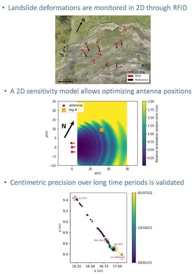
Figure 1.
(Top) The Harmalière landslide location in France. (Bottom) Overview of the Harmalière landslide, with the RFID tag distribution (red points). Blue points: antennas and acquisition system. The dotted black line represents the landslide scar, the gray dotted lines represent 1-m isolines.
Figure 1.
(Top) The Harmalière landslide location in France. (Bottom) Overview of the Harmalière landslide, with the RFID tag distribution (red points). Blue points: antennas and acquisition system. The dotted black line represents the landslide scar, the gray dotted lines represent 1-m isolines.

Figure 2.
Localization error shape at the position of tag A (see Figure 1) compared with the RFID position estimation during a stable period in the Harmalière (November to December 2020). The green point distribution is computed through the transformation (see Equation (6)), using a Gaussian phase distribution with a standard deviation of 0.04 rad. The eigenvectors of the green distribution (red lines) are scaled up to encompass 97% of the data. The black points correspond to the RFID-phase localization results. The antenna positions are set as in the real experiment (see Figure 1).

Figure 3.
Schematic definition of the two-ray multipath model. The orange line represents the line-of-sight path with angle and propagation distance . The blue line represents the reflected path with angle and propagation distance . and are the tag and antenna heights above ground.
Figure 3.
Schematic definition of the two-ray multipath model. The orange line represents the line-of-sight path with angle and propagation distance . The blue line represents the reflected path with angle and propagation distance . and are the tag and antenna heights above ground.

Figure 4.
Schematic description of the matrix transformations in phase space towards real 2D space for a 2-antenna system. (a) Representation of the simulated multipath-induced phase measurement distribution (orange) compared to the previously assumed centered distribution (blue), highlighting the scaling S and translation T. The translation is illustrated by the shift between the center of the blue distribution and the center of the red distribution. (b) True space localization spot obtained by further transformation via the matrix. The antennas are not represented. The systematic bias is again illustrated by the shift between the real position (black point) and the center of the measured distribution (red point).

Figure 5.
Mapping of the 2D localization error extracted from Equations (14) and (15), simulating the geometry of the Harmalière setup. The red dots represent the reader antennas, and the arrows show the principal antenna directions. The orange cross indicates the position of tag A. The vectors ) define the cylindrical coordinate system used later on. (a) The colormap shows the random localization error (maximum dimension of the localization spot) up to 2 cm, related to the phase random deviation . The localization bias is not shown. (b) Color-mapping of the systematic localization bias (related to ) in the xOy plane shows oscillations with meter-order spatial frequency and increasing amplitude with distance from the measurement system. The random localization error is not shown. (c) Color-mapping of the systematic localization bias in the xOz plane, with higher oscillation amplitude and frequency. The ground is located at z= −3 m.

Figure 6.
Unwrapped phase variation for tag A, measured by four antennas at a frequency f = 865 MHz, from January 2021 to February 2022. The grey bar shows a period of missing data due to hardware failure. Data was directly available after replacement of the malfunctioning device.
Figure 6.
Unwrapped phase variation for tag A, measured by four antennas at a frequency f = 865 MHz, from January 2021 to February 2022. The grey bar shows a period of missing data due to hardware failure. Data was directly available after replacement of the malfunctioning device.

Figure 7.
Schematic view of the workflow used to estimate the localization error and bias in the real-scenario Harmalière geometry.
Figure 7.
Schematic view of the workflow used to estimate the localization error and bias in the real-scenario Harmalière geometry.

Figure 8.
RFID localization in the xOy plane, using phase data for tag A (Figure 6). The total displacement is about 1.6 m. The color plot represents the time evolution of the RFID relative localization. The red crosses represent the reference measurements using a tacheometer, with an estimated error of about 4 cm. The tacheometer measurement of March 2021 is set as an absolute reference for relative localization. The black crosses correspond to the estimated random error bars for TD-phase localization (calculated via the model developed in Section 4.2).

Figure 9.
Cumulative 2D displacement norm for each tag, with reference measurements performed via tacheometer (black crosses). An offset was added to every plot to increase readability. The total displacement values are given in Table 3.
Figure 9.
Cumulative 2D displacement norm for each tag, with reference measurements performed via tacheometer (black crosses). An offset was added to every plot to increase readability. The total displacement values are given in Table 3.

Figure 10.
Vector mapping of the total 2D displacement for all available tags from January 2021 to September 2021. The scale is modified for clarity with a 1 m displacement reference (black arrow). The red arrows represent the displacement estimated from the RFID measurements, and the black arrows represent the displacement computed from reference measurements. The blue points numbered 1 to 4 correspond to the reader antennas.

Table 1.
(Up) Geometrical parameters for the positions of the four antennas in the Harmalière setup. (Down) Values of the main variables used in the two-ray model (see Figure 3); the height of the station is relative to the ground at the same position.
Table 1.
(Up) Geometrical parameters for the positions of the four antennas in the Harmalière setup. (Down) Values of the main variables used in the two-ray model (see Figure 3); the height of the station is relative to the ground at the same position.
| Antenna No. | x (m) | y (m) | z (m) |
|---|---|---|---|
| 1 | 0 | 0 | 0 |
| 2 | 0.018 | −0.034 | 1.55 |
| 3 | 0.013 | −2.608 | 0.256 |
| 4 | −0.338 | 2.148 | 0.287 |
| (m) | 3 | ||
| (m) | 1 | ||
| Ground relative permittivity | 2.4 | ||
Table 3.
Total 2D displacement norm for all presented tags computed from the RFID phase, from January 2021 to February 2022. The reference is computed from the tacheometry measurements, with an estimated error of ±4 cm.
Table 3.
Total 2D displacement norm for all presented tags computed from the RFID phase, from January 2021 to February 2022. The reference is computed from the tacheometry measurements, with an estimated error of ±4 cm.
| Tag | 51 | A | 4e | 26 | 55 | 5f | 2d | 5c | 59 | 5b |
|---|---|---|---|---|---|---|---|---|---|---|
| Total disp (m) | 1.54 | 1.37 | 1.20 | 0.81 | 0.75 | 0.85 | 0.69 | 0.67 | 0.74 | 0.56 |
| Reference (m) | 1.57 | 1.45 | 1.28 | 0.81 | 0.79 | 0.74 | 0.77 | 0.74 | 0.72 | 0.59 |
Publisher’s Note: MDPI stays neutral with regard to jurisdictional claims in published maps and institutional affiliations. |
© 2022 by the authors. Licensee MDPI, Basel, Switzerland. This article is an open access article distributed under the terms and conditions of the Creative Commons Attribution (CC BY) license (https://creativecommons.org/licenses/by/4.0/).
Share and Cite
MDPI and ACS Style
Charléty, A.; Le Breton, M.; Larose, E.; Baillet, L. 2D Phase-Based RFID Localization for On-Site Landslide Monitoring. Remote Sens. 2022, 14, 3577. https://doi.org/10.3390/rs14153577
AMA Style
Charléty A, Le Breton M, Larose E, Baillet L. 2D Phase-Based RFID Localization for On-Site Landslide Monitoring. Remote Sensing. 2022; 14(15):3577. https://doi.org/10.3390/rs14153577
Chicago/Turabian StyleCharléty, Arthur, Mathieu Le Breton, Eric Larose, and Laurent Baillet. 2022. "2D Phase-Based RFID Localization for On-Site Landslide Monitoring" Remote Sensing 14, no. 15: 3577. https://doi.org/10.3390/rs14153577
Note that from the first issue of 2016, this journal uses article numbers instead of page numbers. See further details here.