Modelling and Assessment of Single-Frequency PPP Time Transfer with BDS-3 B1I and B1C Observations

Abstract

BDS-3 is now providing global positioning, navigation and timing (PNT) services. BDS-3 has new B1C, B2a and B2b signals compared to BDS-2. This work presents two single-frequency (SF) PPP time transfer models using BDS-3, B1C and B1I observations, and studies the performance of BDS-3 SF PPP time transfer by using 30-day data of 10 globally distributed stations from a multi-GNSS experiment (MGEX). We found that the ionospheric constraint SF PPP (SF1) time transfer model outperforms the method of SF PPP with the receiver clock offset at first epoch as the datum (SF2). Importantly, the statistical uncertainty of SF1 was less than 1 nanosecond, with (0.75, 0.71) ns in the average scheme for all time-links, using both B1I and B1C observations, respectively. The frequency stability of SF1 with B1C observations was improved from 1.73% to 13.04% in the short-term and from 0.88% to 17.49% in the long term, compared to that of B1I for all time-links. Hence, SF1 with B1C observations was recommended for SF PPP time transfer.

1. Introduction

BDS in China has officially provided PNT services for the world since July 2020 [1,2]. Compared to GPS, the BDS-3 adds many new features such as PPP-B2b service [3] and short-message communication devices [4]. In addition, BDS-3 provides B1C and B2a signals for improving compatibility with GPS and Galileo signals, in addition to B2b signals [5,6].

With the successful construction of the BDS-3, it has since been applied in different fields [7,8,9]. Interestingly, the code biases at the satellite ends, as pointed out by Wanninger and Beer [10] in BDS-2 satellites, have been removed from the signals of BDS-3 [11]. This will significantly improve the performance in many precision applications, such as time transfer. Jiao et al. [12] evaluated the BDS-2/3 broadcast ephemeris and concluded that the RMS of BDS-3 broadcast orbit errors were much improved with respect to BDS-2 satellites in all RAC directions. For orbit determination, Zeng et al. [13] investigated the POD with the uncombined GPS and BDS-3 observations. The assessments of SPP/RTK/PPP, ephemeris and new signal for BDS-3 were presented by Shi et al. [14] in detail. They again confirmed that BDS-3 outperformed BDS-2. For precise positioning with QF observations, Li et al. [15] studied the benefit of the QF signals of BDS-3 in ambiguity resolutions and positioning. The results suggested that the accuracy of ERTK positioning was about 1 m in the horizontal direction using IF EWL observations for a 300 km baseline. The performance of PPP with single-, dual-, triple- and quad-frequency observations was evaluated by Jin and Su [16]. They found that the BDS PPP would be greatly enhanced with the use of multi-frequency observations. Then, the PPP-RTK [17] with combined BDS-2/3 and GPS satellites was studied by Li et al. [18]. They showed that high-accuracy positioning services in Europe could be provided by BDS-only positioning in its current state. More interestingly, a real-time PPP in high-precision positioning applications based on the SMC technique was investigated by Nie et al. [4]. The SMC is a unique function of BDS, which can resolve the problem of implementing real-time PPP without a network by other GNSS constellations. Nie et al. [4] suggested that teal-time PPP could reach 3D positioning accuracy of 0.116 m in the offshore experiment using the SMC technique to deliver corrections. In addition, another beneficial feature of BDS-3 is that it provides PPP-B2b services, a special feature that no other navigation systems currently have [1]. Tao et al. [3] analysed the PPP-B2b service and compared it with real-time products from CNES. The results illustrated that the BDS-3 PPP-B2b presented better completeness and availability than the CNES in Asia. The performance of B1C/B2a and B1I/B2I IF combination PPP with BDS-3 satellites based on PPP-B2b service was further studied by Xu et al. [19], indicating that real-time kinematic PPP with B1C/B2a could achieve 27.8 cm and 36 cm in horizontal and vertical directions after convergence, whilst for B1I/B3I they are 53 cm and 42.8 cm.

In addition to high precision positioning, BDS-3 satellites are also employed to determine time transfer. PPP time transfer with TF observations was presented by Su and Jin [20]. They suggested that the stability and accuracy of BDS-3 TF PPP time transfer was identical to that of DF PPP. Ge et al. [21] presented different DF IF combination PPP models with QF BDS-3 observations for time transfer. The performance of BDS-3 time transfer with the CV, AV and PPP models in terms of accuracy and instability was investigated by Guang et al. [22]. They found that the uncertainty stability of BDS-3 B1C/B2a IF combination reached 0.36 ns and 0.8 ns with CV and AV models, respectively, and BDS PPP time transfer using B1I/B3I IF combination was similar to GPS L1/L2. Ge et al. [23] studied the PPP time transfer with BDS-3/Galileo QF observations. Their experiment demonstrated that the redundancy and reliability of PPP time transfer could be enhanced with QF observations, in regards to the DF observations. In addition, real-time PPP time transfer was further investigated by Ge et al. [24] and it was found that the stability of real-time PPP with BDS-3 achieved 1E-15 at 122,880 s. However, the above research mainly uses dual- or multi-frequency observations to achieve PPP time transfer. Ge et al. [25] further presented a multi-GNSS SF PPP time transfer model. They suggested that SF PPP with the GIM constraint, called SF1 in our work, presented the best performance compared to other SF PPP models. However, no research has so far studied the SF PPP time transfer with BDS-3 satellites, especially using B1C observations, at present. In addition, Zhang et al. [26] introduced an SF model with no external constraints, which is called SF2 in our work, and this model has not yet been applied or evaluated for time transfer. Hence, the SF1 and SF2 time models were first studied and assessed with BDS-3 B1I observations. Then, to evaluate the performance of both models, the SF PPP time transfer using B1C and B1I observations was investigated and compared by in-depth analysis.

The organization of our work was as follows. Two SF PPP models and the principles of time transfer are introduced in Section 2. Then, the processing strategies and dataset are presented in Section 3. Section 4 covers the comparison of two SF PPP models and the results of the SF PPP time transfer using B1C and B1I. Finally, the main conclusions of our work are summarized in Section 5.

2. Methods

Firstly, the general observations for SF pseudorange and carrier phase observations were outlined. Then, two SF PPP models were introduced. Additionally, the principle of SF PPP time transfer was exhibited.

2.1. Observations

The SF uncombined observations are introduced as [27,28,29]

$$\{\begin{array}{l}{p}_{r,1}^s(i)={\rho }_{r,1}^s(i)+d{t}_r(i)-d{t}^s(i)+m_r^s\cdot Z_r(i)+I_{r,1}^s(i)+b_{r,1}-b_1^s+{\xi }_r^s(i)\\ l_{r,1}^s(i)={\rho }_{r,1}^s(i)+d{t}_r(i)-d{t}^s(i)+m_r^s\cdot Z_r(i)-I_{r,1}^s(i)+{\lambda }_1^s\underset{N_{r,1}^s}{\underbrace{(n_{r,1}^s+d_{r,1}-d_1^s)}}+{\varsigma }_{r,1}^s(i)\end{array}$$

(1)

where $p$ and $l$ illustrate pseudorange and carrier phase observations; s and r indicate the satellites and receivers; $d{t}_r(i)$ and $d{t}^s(i)$ represent the receiver and satellites clock offsets at epoch i; $m_r^s$ and $Z_r(i)$ are the mapping function and ZTD at station r. $I_{r,1}^s(i)$ is the slant ionospheric delay; $b_{r,1}$ and $b_1^s$ denote the receiver and satellite code biases, respectively. ${\lambda }_1^s$ and $N_{r,1}^s$ are the wavelength of the carrier phase in the L1 band and the float ambiguity for absorbing the phase hardware delays from both receiver $d_{r,1}$ and satellite $d_1^s$ ends; ${\xi }_r^s(i)$ and ${\varsigma }_{r,1}^s(i)$ are the pseudorange and carrier phase noises at epoch i.

Generally, the precise clock products released from IGS are referred to as DF IF combination. By applying the precise products, the SF PPP observations can be rewritten as

$$\{\begin{array}{l}\Delta p_{r,1}^s(i)={\overrightarrow{e}}_r^s\cdot \overrightarrow{\Delta }x+\underset{\overline{d}{t}_r(i)}{\underbrace{[d{t}_r(i)+b_{r,1}^{}]}}+m_r^s\cdot Z_r(i)+\underset{{\overline{I}}_r^s(i)}{\underbrace{[I_{r,1}^s(i)+\frac{f_2^2}{f_1^2-f_3^2}(b_1^s-b_3^s)]}}+{\xi }_r^s(i)\\ \Delta l_{r,1}^s(i)={\overrightarrow{e}}_r^s\cdot \overrightarrow{\Delta }x+\overline{d}{t}_r(i)+m_r^s\cdot Z_r(i)-{\overline{I}}_r^s(i)+\underset{{\overline{N}}_{r,1}^s}{\underbrace{[{\lambda }_1^s{N}_{r,1}^s-b_{r,1}^{}+\frac{f_2^2}{f_1^2-f_3^2}(b_1^s-b_3^s)]}}+{\varsigma }_{r,1}^s(i)\end{array}$$

(2)

where $\Delta p_{r,1}^s(i)$ and $\Delta l_{r,1}^s(i)$ are the OMC at the pseudorange and carrier phase, respectively. ${\overrightarrow{e}}_r^s$ indicates the unit vector. $\overrightarrow{\Delta }x$ is the vector of receiver coordinates. f represents the frequency. Note the reference of precise clock products for BDS-3 is B1I/B3I IF combination. Here, f₁ and f₃ indicate the frequencies of B1I/B3I or B1C/B2a.

2.2. SF1

Obviously, Equation (2) is rank-deficient. Here, the GIM model with IGS ionospheric products was used to constrain SF PPP, called SF1 in our work. Then, the SF PPP time transfer model is written as:

$$\left[\begin{array}{c}\Delta p_{r,f}^{1,}\\ \Delta l_{r,f}^1\\ ⋮\\ \Delta p_{r,f}^m\\ \Delta l_{r,f}^m\\ {\overline{I}}_{r,f}^1\\ ⋮\\ {\overline{I}}_{r,f}^m\end{array}\right]=\left[\begin{array}{ccccc}{e}_r& 1& M& I& R_1\\ U& U& U& K& U\end{array}\right]\left[\begin{array}{c}\Delta \overrightarrow{x}\\ \overline{d}{t}_r\\ Z_r\\ {\overline{I}}_{r,1}^s\\ {\overline{N}}_{r,1}^s\end{array}\right]+\left[\begin{array}{l}{\xi }_{r,1}^s\\ {\varsigma }_{r,1}^s\\ {\epsilon }_{r,ion}^s\end{array}\right]$$

(3)

where $U$ indicates the zero matrix; $K$ is the identity matrix; ${\overline{I}}_{r,1}^m$ indicates the slant ionospheric delay from the GIM model. I is the unit matrix. $R_1$ is the coefficient matrix of the ambiguity parameters. ${\epsilon }_{r,ion}^s$.

The ionospheric observations were heavier at the beginning of SF PPP due to the accuracy of ionospheric products, but their weight was reduced after convergence. Here, the progressive relaxation constraint as used in [30] is applied:

$${\sigma }_{{\epsilon }_{r,\mathrm{ion}}^s}^2(i)={\sigma }_{{\epsilon }_{\mathrm{ion}},0}^2+\alpha (i-1)\Delta T$$

(4)

$\alpha$ indicates the change rate of variance; $\Delta T$ is the sample interval; ${\sigma }_{{\epsilon }_{\mathrm{ion}},0}^2$ and $\alpha$ are generally set as 0.09 m² and 0.04 m²/min [30].

2.3. SF2

Zhang et al. [26] presented an SF PPP method without using the virtual ionospheric observations. The receiver clock offset at the first epoch was set as the datum to eliminate the correlation of the ambiguities, slant ionosphere and receiver clock offset. Then, the full-rank SF PPP model for epoch 1 and i = 2, 3 k can be written as follows:

$$\{\begin{array}{l}\Delta p_{r,1}^s(1)={\overrightarrow{e}}_r^s\cdot \overrightarrow{\Delta }x+m_r^s\cdot Z_r(1)+\underset{{\widehat{\overline{I}}}_r^s(1)}{\underbrace{[{\overline{I}}_r^s(1)+\overline{d}{t}_r(1)]}}\\ \Delta p_{r,1}^s(i)={\overrightarrow{e}}_r^s\cdot \overrightarrow{\Delta }x+\underset{\Delta \overline{d}{t}_r(i)}{\underbrace{[\overline{d}{t}_r(i)-\overline{d}{t}_r(1)]}}+m_r^s\cdot Z_r(i)+{\widehat{\overline{I}}}_r^s(i)\\ \Delta l_{r,1}^s(1)={\overrightarrow{e}}_r^s\cdot \overrightarrow{\Delta }x+m_r^s\cdot Z_r(1)-{\widehat{\overline{I}}}_r^s(1)+\underset{{\widehat{\overline{N}}}_{r,1}^s}{\underbrace{[{\overline{N}}_{r,1}^s+2\overline{d}{t}_r(1)]}}\\ \Delta l_{r,1}^s(i)={\overrightarrow{e}}_r^s\cdot \overrightarrow{\Delta }x+\Delta \overline{d}{t}_r(i)+m_r^s\cdot Z_r(i)-{\widehat{\overline{I}}}_r^s(i)+{\widehat{\overline{N}}}_{r,1}^s\end{array}$$

(5)

Equation (6) shows the full-rank uncombined SF PPP functional model and depicts the parameters to be estimated. We find that the receiver clock offsets that were estimated starting from the second epoch are the receiver clock difference between the current epoch and the first epoch. The estimated slant ionosphere delay and ambiguities are all biased by a constant receiver clock offset at the first epoch [31]. Hence, SF2 can be applied for frequency transfer without knowing the receiver clock offset at first epoch but can be applied for time transfer if the receiver clock offset at first epoch is known.

2.4. Time Transfer

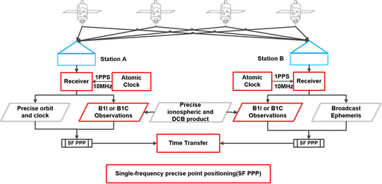
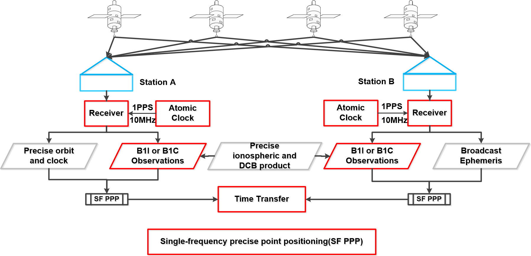
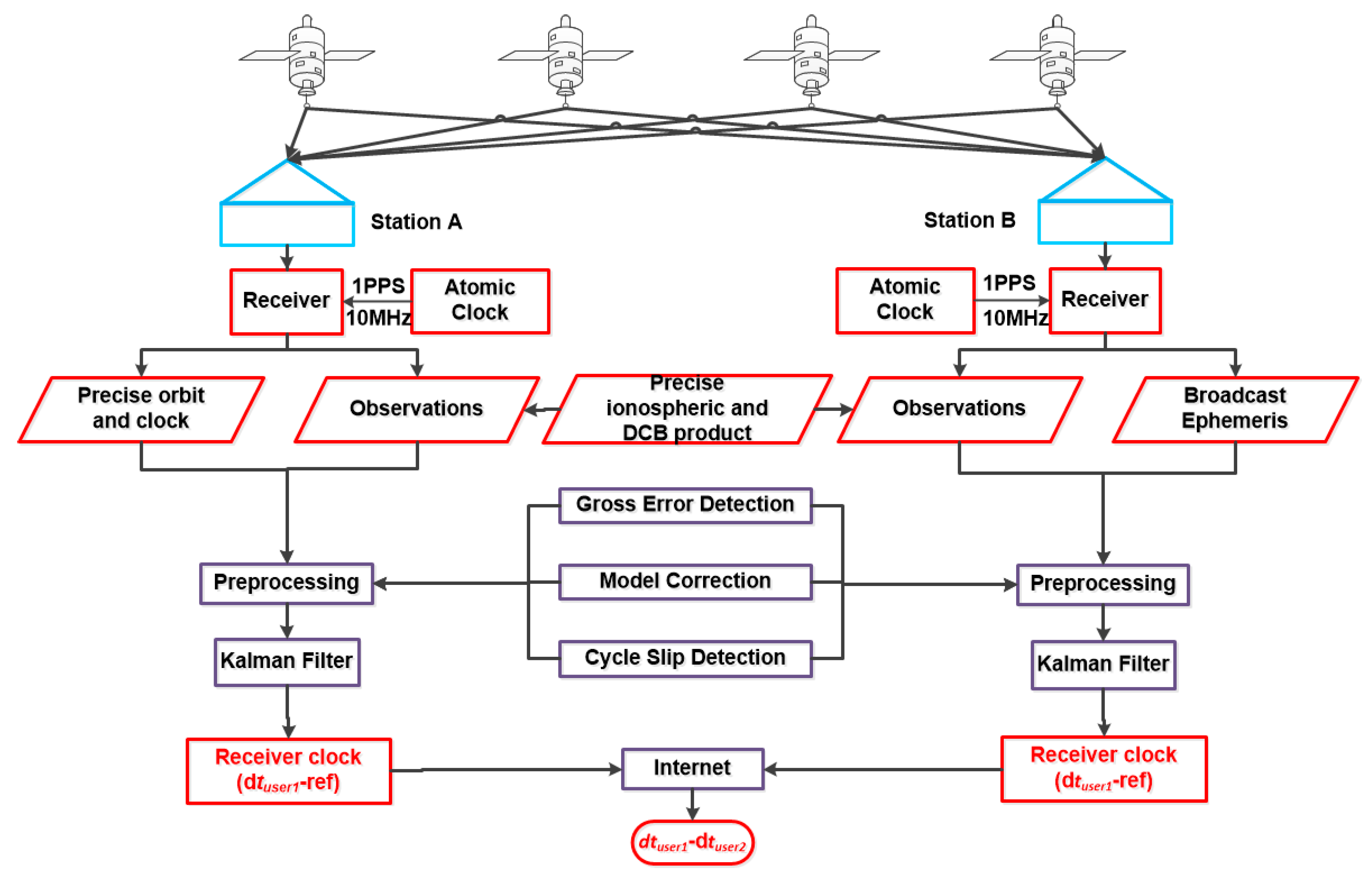
A flowchart of the SF PPP time transfer is exhibited in Figure 1. Station A and B were both connected to the local atomic clocks. The observations and broadcast ephemeris from the receivers and the precise orbit/clock products, ionospheric/DCB products were prepared first. Then, the SF PPP model was used to estimate the receivers’ clock offsets after gross error detection, model correction, cycle slip detection, etc. The receiver clock offsets are calculated as follows for stations A or B:

$$T_A=t_{user1}-t_{ref}$$

(6)

$$T_B=t_{user2}-t_{ref}$$

(7)

where $T_A$ and $T_B$ refer to the receiver clock offsets; $t_{user1}$ and $t_{user2}$ are the local time. $t_{ref}$ illustrates the reference of the precise clock products from IGS.

Then, the difference $\Delta T$ between station A and B, can be expressed as:

$$\Delta T=T_B-T_A$$

(8)

3. Processing Strategies and Experimental Data

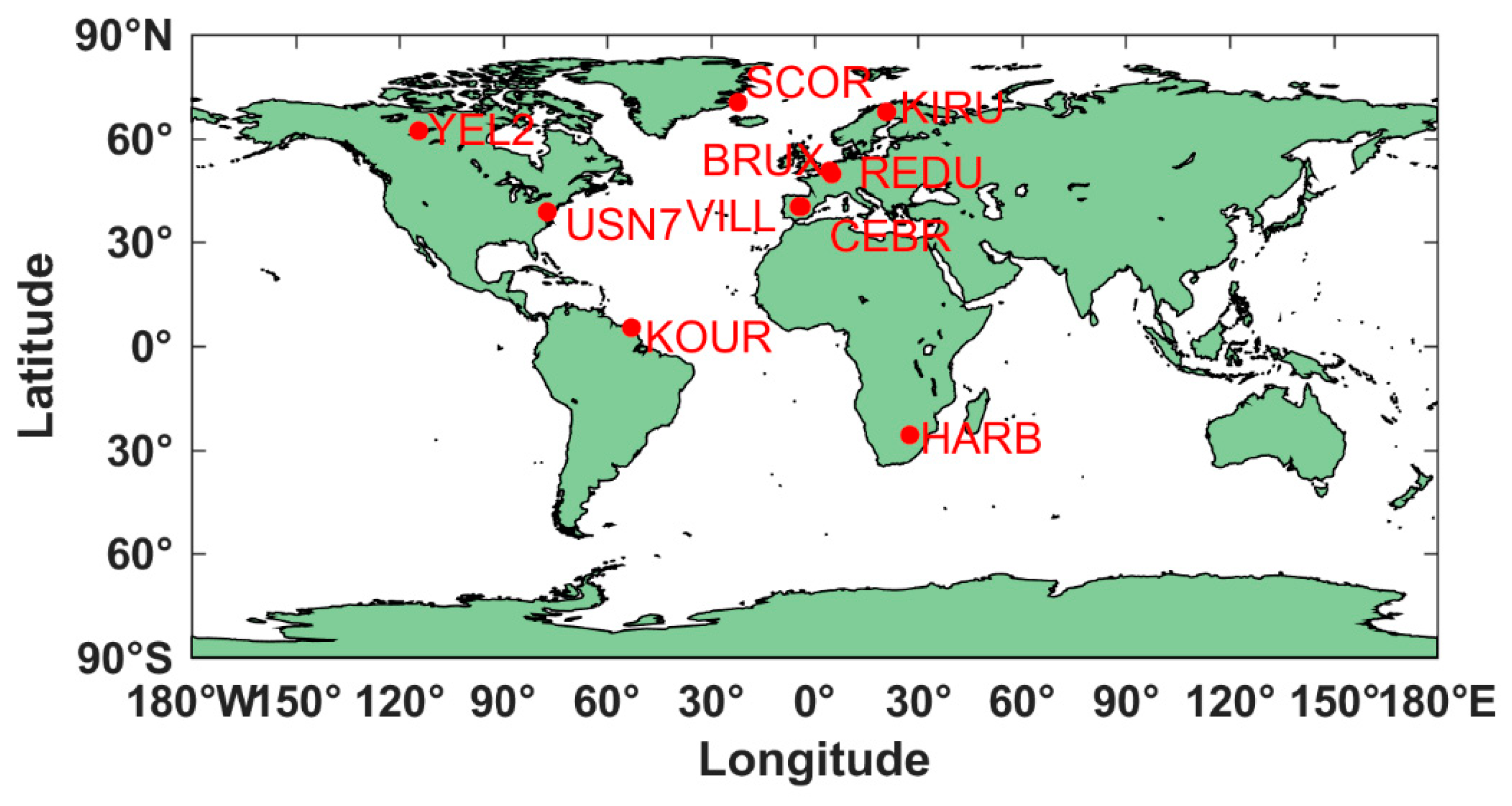
To study the performance of BDS-3 SF PPP time transfer using B1I or B1C signals, 10 stations from MGEX were chosen and tested. In this work, BRUX was set as the central node because an atomic clock was connected. Nine time links were then presented. The observations are from DOY 30 to 60, 2021. Precise orbit/clock products are from GFZ, the ionosphere products were attained from IGS. The locations of the selected stations are exhibited in Figure 2. A summary of all the stations is listed in

Table 1. A summary of stations for the SF PPP time transfer with BDS-3 B1C/B1I observations.

Station	Receiver	Antenna	Clock
CEBR	SEPT POLARX4	SEPCHOKE_MC	H-MASER
HARB	TRIMBLE NETR9	TRM59800.00	CESIUM
REDU	SEPT POLARX4	SEPCHOKE_MC	CESIUM
SCOR	JAVAD TRE_G3TH SIGMA	ASH701941.B	RUBIDIUM
VILL	SEPT POLARX4	SEPCHOKE_MC	CESIUM
USN7	ASHTECH Z-XII3T	TPSCR.G5	H-MASER
KIRU	SEPT POLARX4	SEPCHOKE_MC	CESIUM
KOUR	SEPT POLARX4	SEPCHOKE_MC	H-MASER
BRUX	SEPT POLARX4TR	JAVRINGANT_DM	UTC(ROB)
YEL2	SEPT POLARX4TR	LEIAR25.R4	H-MASER

, which includes information for receiver, antenna and external atomic clock. In addition, our work will be tested with the development of GAMP software [29].

Two experiments were designed for the BDS-3 SF PPP approach, using B1I and B1C observations and the GBM/IGS products. First, time transfer performance of SF1 and SF2 with B1I observation were compared. Second, the better SF PPP model using B1I/B1C observations were tested to prove the characteristic of BDS-3 SF PPP time transfer with two observations.

Table 2. BDS-3 SF PPP processing strategies.

Scheme	Strategies
Estimation method	Kalman filter
Signal selected	BDS-3: B1I and B1C
Sampling rate	30 s
Phase wind-up	Modified [32]
Tropospheric delay	ZHD: modified by models [33]
	ZWD: estimated using GMF [34]
Tidal displacement	Modified [35]
Cut-off angle	10°
Sagnac effect	Modified [35]
Station coordinates	Fixed
Relativistic effect	Modified [35]
PCV and PCO	igs14.atx
Phase ambiguities	Estimate as constant
DCB	DLR
Receiver clock offset	White noise
Ionospheric delay	White noise

presented processing strategies for the BDS-3 based SF PPP.

4. Results

We begin this section by introducing a comparison of multipath errors of BDS-3 B1I and B1C observations. Then, the two SF PPP models are studied with BDS-3 B1I signals. Furthermore, the characteristic of the BDS-3 SF PPP with B1I and B1C is investigated and presented in detail.

4.1. The Multipath Error Analysis of B1C and B1I Observations

As we know, the quality of observations in pseudorange is very important for PPP convergence and the estimation of the receiver clock offsets. In order to analyse the SF PPP time transfer using B1I and B1C observations, the multipath errors of B1C and B1I pseudorange observations for 9 stations on DOY 30, 2021 were studied in detail. Figure 3 exhibits the multipath errors of 9 stations with B1C and B1I signals for all BDS-3 satellites. The elevation of all BDS-3, which can be observed at each station, is larger than 10° for multipath errors calculation. From the figure, three findings emerge. First, the multipath errors of different stations show obvious differences, which may be caused by the observation environment of different stations. Second, obviously, the lower the height angle, the greater the multipath error for B1I and B1C at all stations. Third, importantly, the RMS values of multipath errors for B1C observations at all stations are smaller than that of B1I observations, and this conclusion is consistent with the conclusions from papers [11,36,37].

4.2. Different SF Model Comparison with B1I Observations

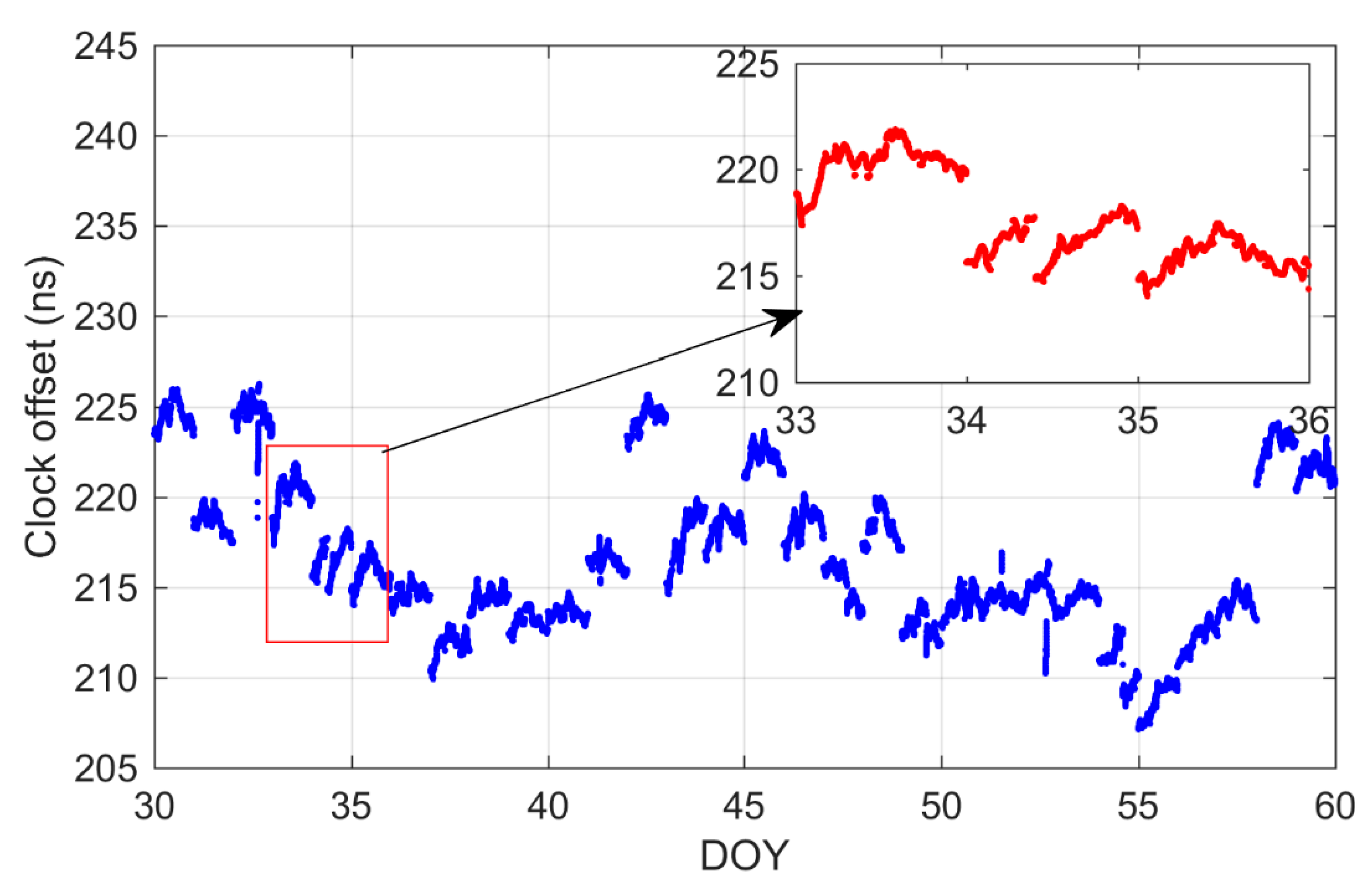
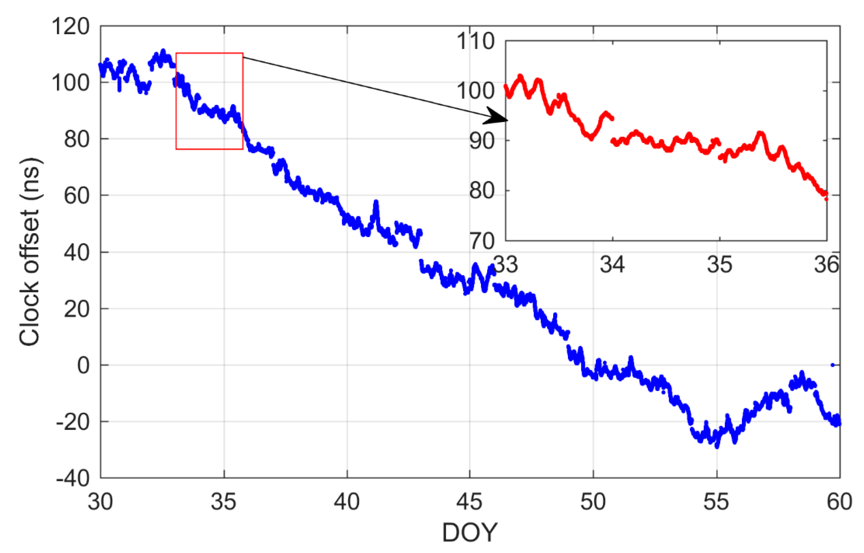
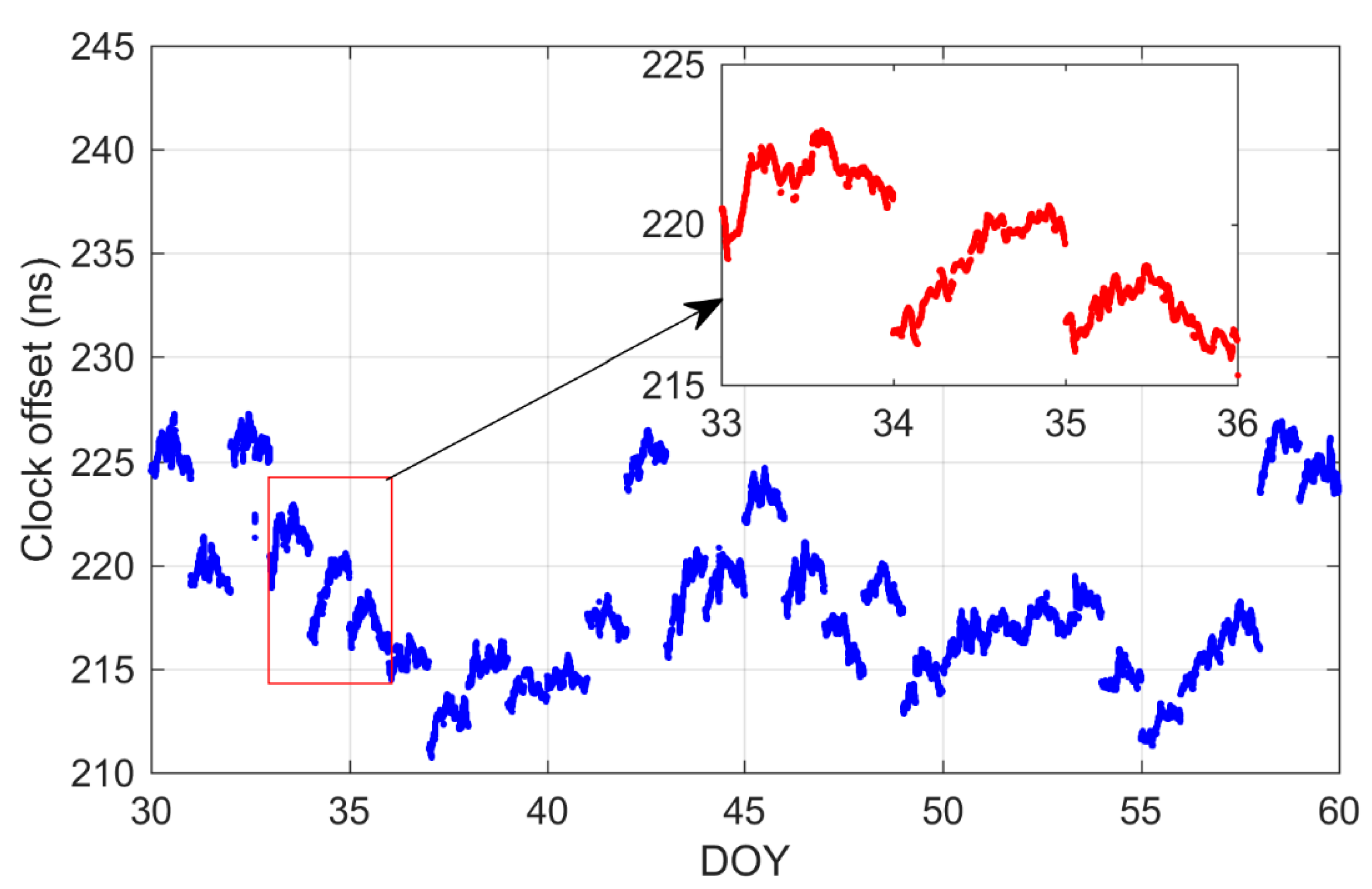
Since Ge et al. [25] have selected the optimal model (SF1) among IF, ionospheric-corrected and SF1 SF PPP time transfer models, we studied the performance of SF1 and SF2 time transfer methods. Figure 4 and Figure 5 exhibit the receiver clock offsets calculated with the SF1 model with B1I for BRUX and REDU stations. In addition, the receiver clock offsets obtained from the SF2 model with B1I observations for BRUX and REDU stations are displayed in Figure 6 and Figure 7. By comparing the four figures, four preliminary conclusions were drawn, which will be outlined later. First, obvious jumps in the daily time series in both SF1 and SF2 methods were found, especially at BRUX station. Usually, the time series of an atomic clock in the timing lab is generally stable, such as that of BRUX station, which is connected to UTC (ROB). Hence, the jumps in the receiver clock offsets are mainly caused by the datum of precise satellite clock products. At present, the datum of precise satellite clock is aligned to the broadcast GPS time for GPS-only at GBM products, while the references for other satellite system clocks, such as BDS, GLONASS and Galileo are not imputed to a stable time system. Luckily, the reference time of precise clock products will be eliminated for the SF PPP time transfer, see Equations (6)–(8). The second finding is that the values of the receiver clock offset obtained from SF1 and SF2, respectively, are obviously different. However, the trend of the time series from SF1 and SF2 is basically the same. As we pointed out in Equation (6), the receiver clock offsets calculated from the SF2 model absorbed the receiver clock offsets at first epoch. Note that the time series in Figure 6 and Figure 7 add initial values. However, the initial value is not very accurate because we used the initial value of the first epoch calculated by the SF1 model. Thirdly, compared with Figure 4 and Figure 6 or Figure 5 and Figure 7, we can find that the noise levels of the solutions from SF2 are larger than that of SF1, especially in partial magnification. That means SF2 is not as good as SF1. This conclusion will be further proved later. Fourthly, although the noise of SF2 is larger than that of SF1, the short-term fluctuation of its time series is relatively smaller than that of SF1. This may be affected by the characteristics of the ionospheric products used in SF1.

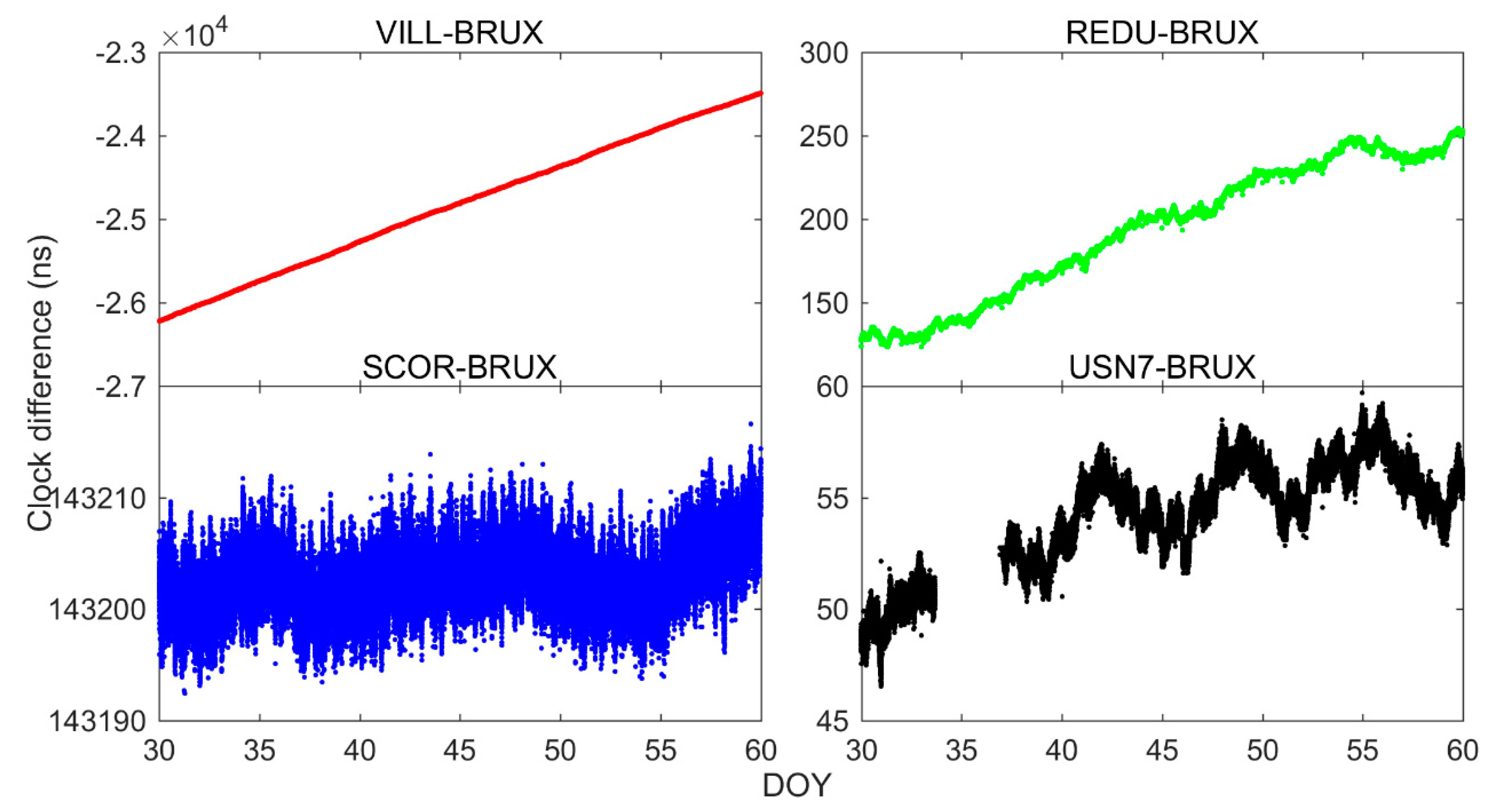
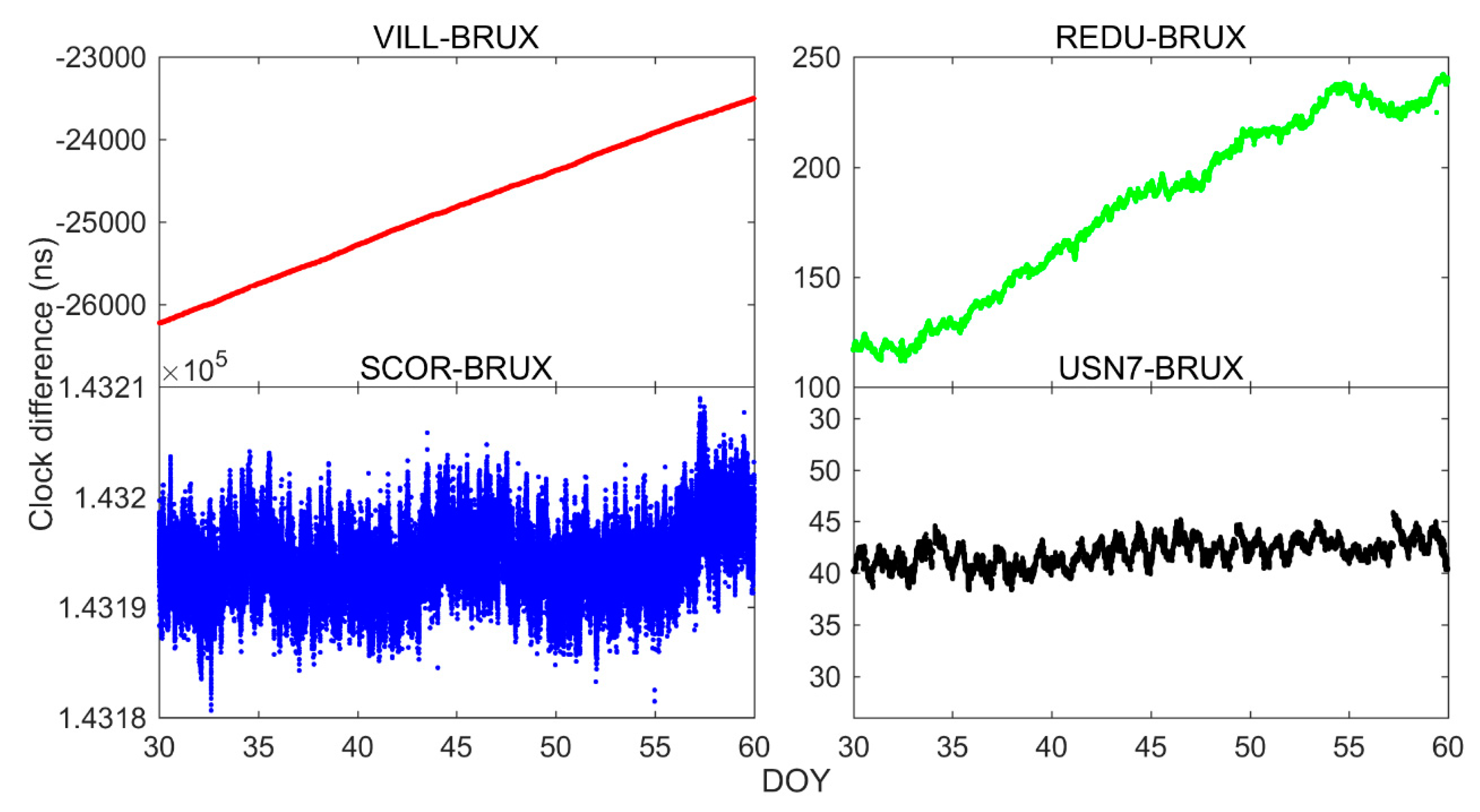
Time transfer usually takes the time difference between two places. Figure 8 and Figure 9 exhibit the time transfer solutions obtained from SF1 and SF2, respectively, for four time links. Note that other time links show similar performance and are not described in detail here. Additionally, part of the time series in the figure is missing due to the loss of observations. Combining two figures, we can draw three initial conclusions. First, for time transfer solutions, the jumps in the receiver clock offsets have completely disappeared, see REDU-BRUX, which further proves that the jumps in the receiver clock offsets were mainly caused by the reference of precise clock products. Secondly, the trend of time transfer with SF2 is similar to that of SF1. Thirdly, the noise of time transfer solutions for USN7 and BRUX with SF2 are larger than that of SF1, which is consistent with the above conclusions.

To further compare the disadvantages and advantages of two SF PPP models, the mean and STD values of the difference between time transfer solutions from SF1 and SF2 models with B1I observations and IGS final clock products are calculated and listed in

Table 3. The mean and STD values of the differences between SF1 and SF2 with B1I observations and IGS final clock product (unit: ns).

	Mean		STD
	SF1	SF2	SF1	SF2
CEBR_BRUX	3.65	−8.16	0.64	0.66
HARB_BRUX	4.93	−5.35	0.90	0.98
KIRU_BRUX	0.17	−7.91	0.64	0.68
KOUR_BRUX	1.45	−4.82	0.93	0.94
REDU_BRUX	0.46	−3.33	0.60	0.82
SCOR_BRUX	17.21	6.10	0.65	0.77
USN7_BRUX	1.13	−7.04	0.90	0.91
VILL_BRUX	4.84	−6.69	0.67	0.68
YEL2_BRUX	3.35	−9.63	0.76	0.77

. We can suggest that, although we correct the initial value, there is still a significant difference between the mean values of SF2 and SF1 solutions, because the exact initial value is still difficult to determine. Therefore, SF2 is not recommended for time transfer. From STD values of the difference in Table 3, two findings were suggested. First, all the STD values of the difference is less than 1 ns. Therefore, it suggests that the SF PPP time transfer with BDS-3 satellites can release sub-nanosecond level. Secondly, the performance of SF1 is slightly better than SF2. Note that the final clock products from IGS are set as the true values here.

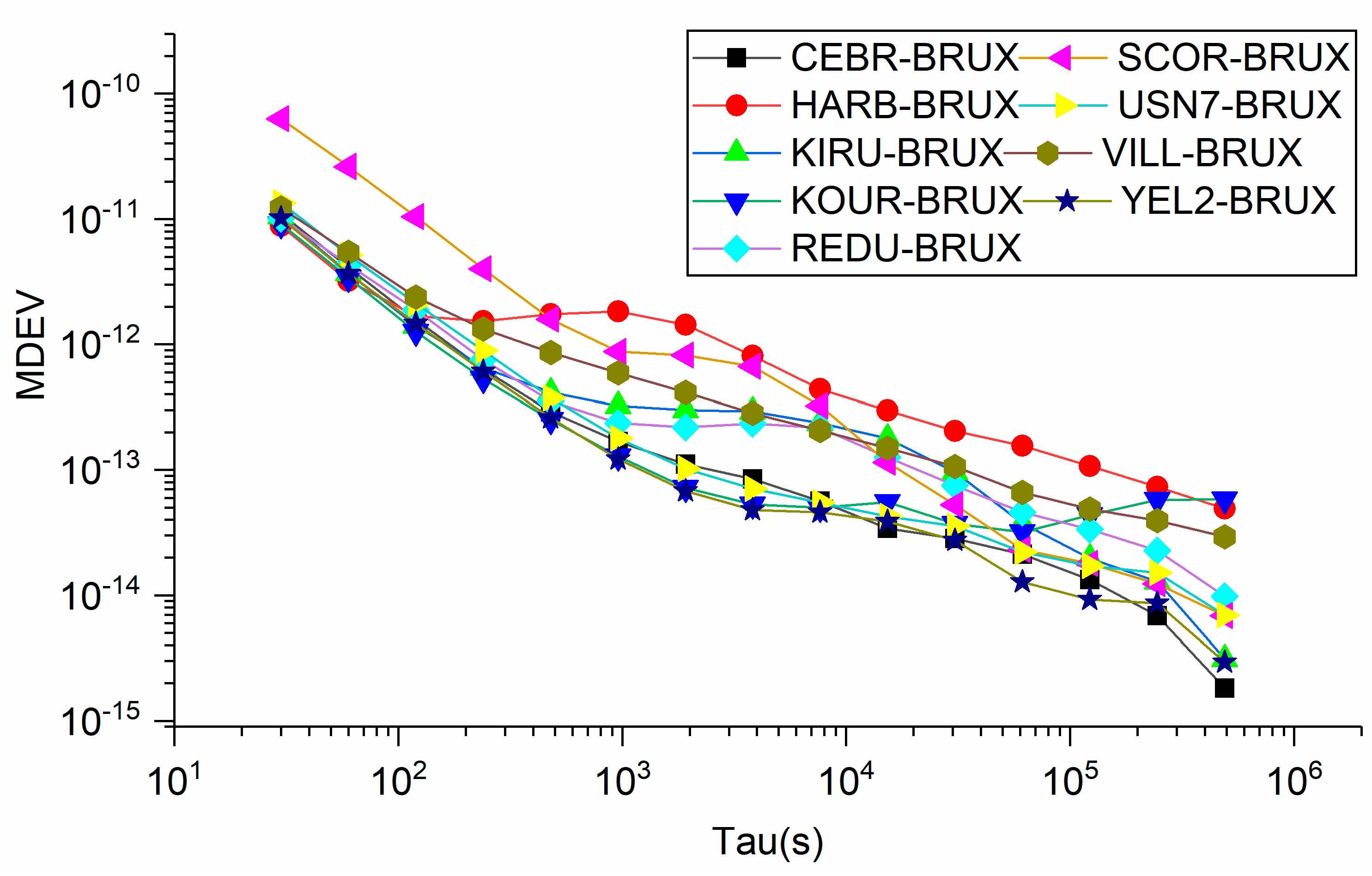
In addition, we further present the MDEV of 9 time links obtained from SF1 and SF2 in Figure 10 and Figure 11, respectively, which can explain the characteristics of the two models in the frequency domain. One finding, which can be observed obviously, is that the short-term frequency stability of SF1 outperforms that of SF2. This can explain our previous finding that the noise of SF2 solutions is larger than that of SF1, while the frequency stability in the long-term exhibits the same performance between the SF1 and SF2 models. More interestingly, we find that the frequency stability of SF2 before 120 s shows a similar performance for all time links, except SCOR-BRUX, while that of SF1 presents a different performance for different stations. This is because the accuracy of ionospheric products is different at different latitudes. Overall, we recommend the SF1 model for time transfer.

4.3. SF PPP Time Transfer with B1C and B1I

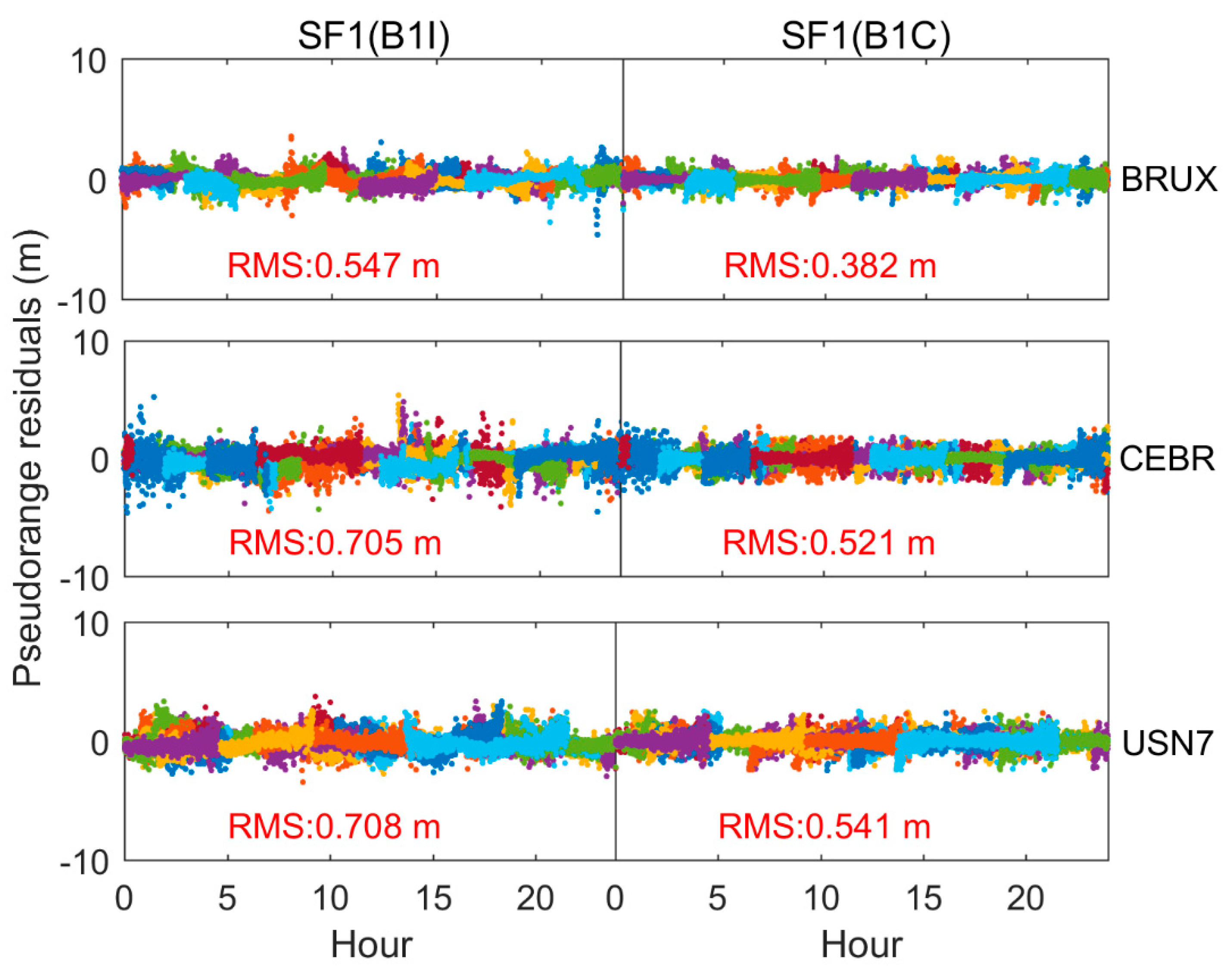
Pseudorange residuals can reflect the performance of PPP from another aspect. Figure 12 exhibits the pseudorange residuals of the SF1 model with B1C and B1I observations for three stations. From the figure, two findings are presented. First, because the reference of precise satellite clock products is an IF ionospheric combination, the DCB correction is required. The pseudorange residuals of SF1 with B1I and B1C did not show significant system differences, indicating the correctness of our method for correcting DCB. Secondly, the RMS of SF1 with B1C is smaller than that of B1I, such as (0.547, 0.382) m for the RMS of SF1 with B1I and B1C, respectively, at BRUX station. This can explain the superiority of SF1 with B1C observations.

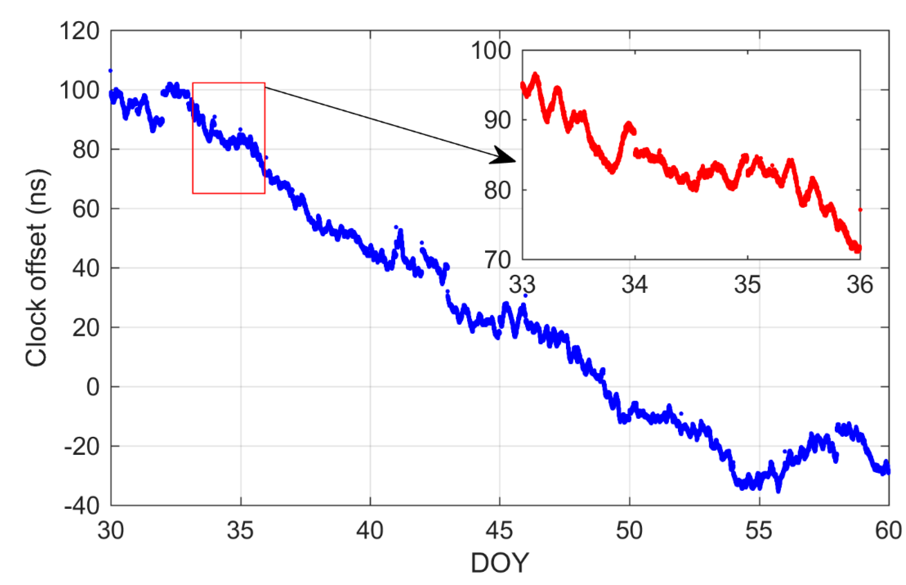
According to the conclusions we have reached, a SF1 model can be employed to study the SF PPP with B1I and B1C observations. Note that time transfer with the SF1 model using B1I has been presented at the above findings. Here, we present the results obtained from SF1 with B1C observations. Figure 13 and Figure 14 display the receiver clock offsets from SF1 with B1C observations for BRUX and REDU stations. According to Figure 4, Figure 5, Figure 13 and Figure 14, we can conclude three suggestions. First, as we mentioned earlier, whether B1I or B1C observation was used, the time series of the clock offset present obvious jumps from day to day. That phenomenon further proves that current product references for BDS-3 clocks are not reduced to a unified time scale at GBM products. Fortunately, it does not affect time transfer or high precision positioning, but it cannot be used for timing. Second, the trend of time transfer with B1I and B1C observations are almost overlapped. Although SF PPP uses different observations (B1I and B1C observations), the difference between the user time and the datum of the product is the same. The only difference is the hardware delay of the different signals at the receiver. Thirdly, compared with the partial enlarged insets in Figure 4 and Figure 13, the receiver clock offset obtained from B1C is continuous throughout the day, whereas that of B1I tends to jump. This suggests the advantage of the B1C observations. This conclusion is further proved in the following section. Additionally, similar to before, the time transfer solutions for four time links obtained from the SF1 model with B1C observations are exhibited in Figure 15 and Figure 8 and Figure 15 are synthesised for overall analysis. The performance of SF1 with B1C at USN7-BRUX time link is better than that of B1I observations, because the time transfer solutions for USN7-BRUX was more continuous and smoother, although the performance of the time transfer results of the other three time links were very similar.

As before, we calculated the mean and STD values of the differences between the solutions from SF1 with B1I and B1C observations and IGS final clock products, the results of which are

Table 4. The mean and STD values of SF1 with B1I and B1C observations (unit: ns). Here, the IGS final clock product was set as the reference. Note that the improvement indicates the performance of SF1 with B1C observations with respect to that of with B1I observations with STD values.

	Mean		STD		Improvement (%)
	B1I	B1C	B1I	B1C
CEBR_BRUX	3.65	4.58	0.64	0.63	1.56
HARB_BRUX	4.93	4.86	0.90	0.85	5.55
KIRU_BRUX	0.17	1.55	0.74	0.71	4.03
KOUR_BRUX	1.45	2.74	0.93	0.89	4.30
REDU_BRUX	0.46	1.34	0.60	0.51	15.00
SCOR_BRUX	17.21	13.48	0.65	0.61	6.15
USN7_BRUX	1.13	1.16	0.90	0.86	4.44
VILL_BRUX	4.84	5.32	0.67	0.63	5.97
YEL2_BRUX	3.35	4.20	0.76	0.75	1.31

. Although it is not clear from the figure, there is an obvious system difference in the time transfer solutions calculated by the SF1 with B1I and B1C observations; it can be seen from the mean value of the differences that there is system bias in the results obtained from different time links calculated by the SF1 with B1I and B1C observations. This system bias for SF1 with B1C and B1I observations can be explained by the fact that the time difference has absorbed the hardware delay at the receiver ends, because the time delays of different signals in hardware are quite different. Additionally, the STD values of the time difference calculated from SF1 with B1I and B1C observations are all less than 1 ns, which is similar to SF1 with GPS L1 or Galileo E1 observations in [25]. Hence, we suggest that the accuracy of SF PPP with B1I and B1C release sub-nanosecond levels.

Ions smaller than that of B1I observations and the improvement of the SF1 model with B1C observations range from 1.3% to 15% with respect to that of B1I observations. Hence, for SF PPP with BDS-3, B1C observations are recommended.

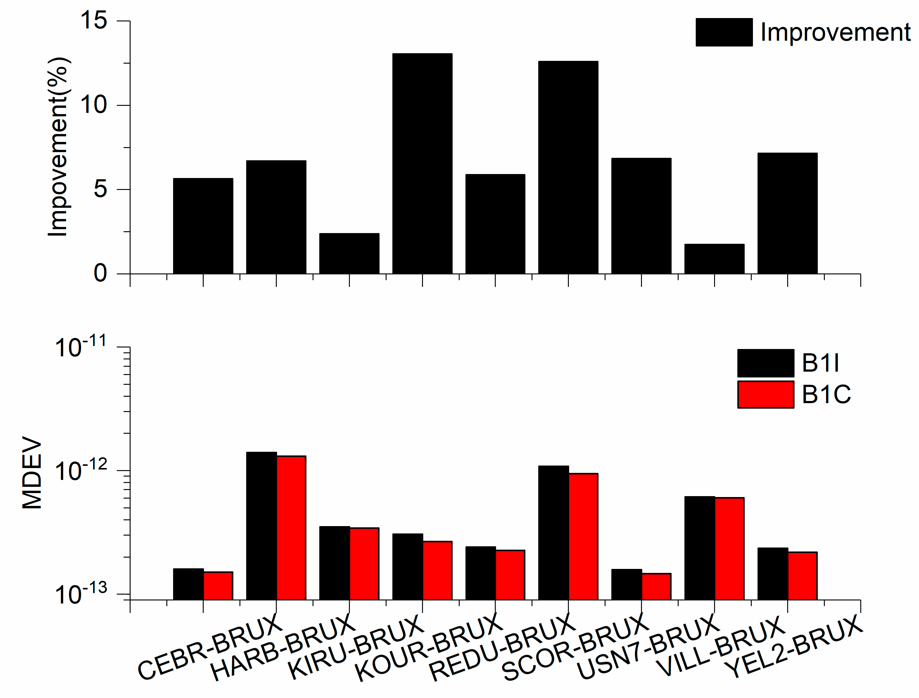
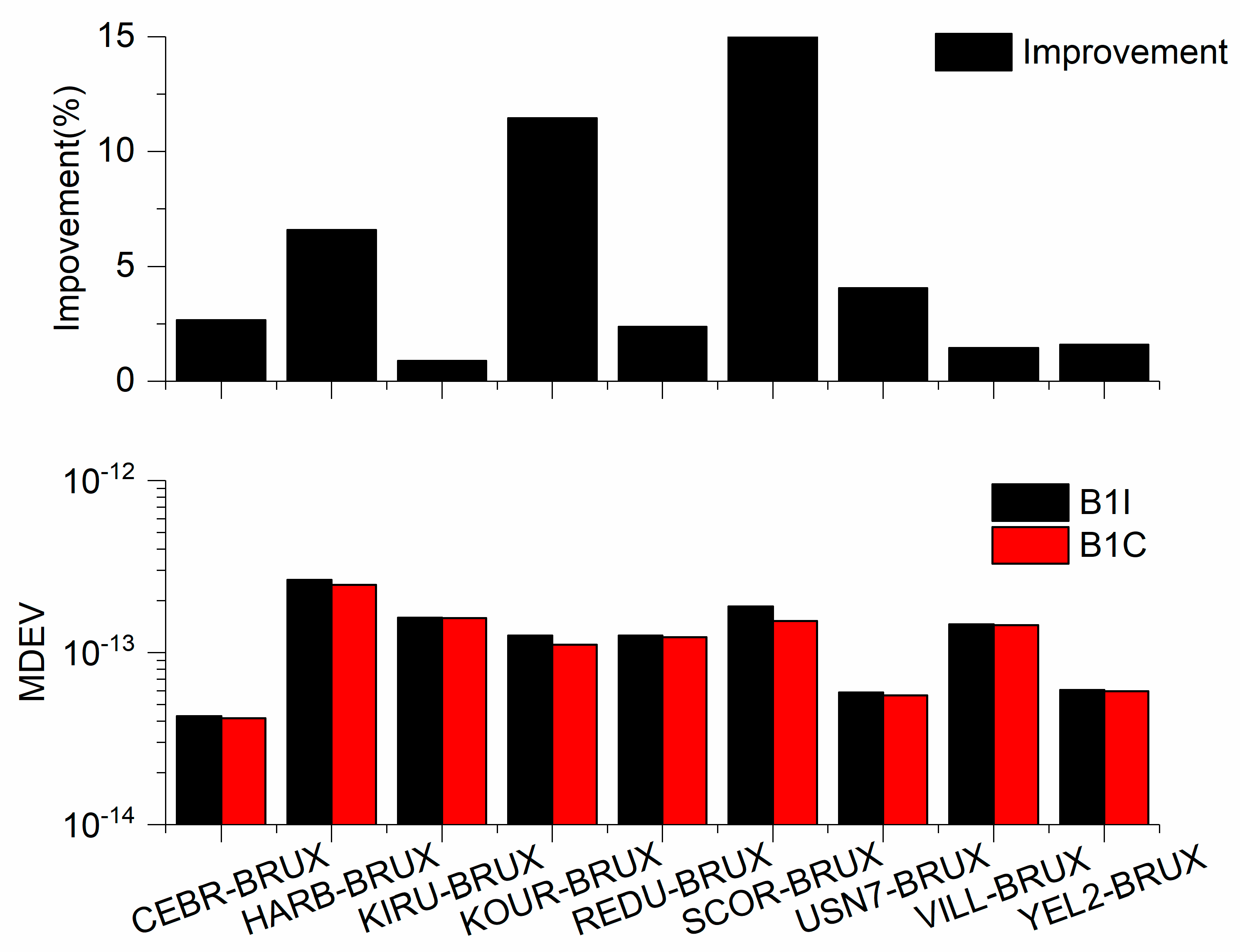
In addition, the MDEV of the 9 time links obtained from the SF1 model with B1C observations is displayed in Figure 16. From the combined Figure 10 and Figure 16, it can be seen that the frequency stability of the SF1 model with B1C and B1I observations can reach a similar level. In order to clearly express the frequency stability short- and long-term, the frequency stability with durations of 960 s and 15,360 s of all time links was exhibited in Figure 17 and Figure 18. The mean frequency stability of 960 s is about 5.01E-13 and 4.67E-13 for B1I and B1C observations. Compared with the short-term frequency stability from B1I observations, the short-term frequency stability of B1C observations was improved from 1.73% to 13.04%. Furthermore, the mean frequency stability at 15,360 s is about 1.29E-13 and 1.21E-13 for B1I and B1C observations. The improvement of B1C ranges from 0.88%to 17.49% with respect to B1I observation.

5. Conclusions

BDS-3 is now capable of providing global PNT services. This study exhibited two single-frequency PPP models with BDS-3 B1I or B1C observations for time transfer and assessed the performance of BDS-3 SF PPP with 30-day observations from 10 stations selected from MGEX networks. Before studying the time transfer, the quality of pseudorange observations for B1I and B1C signals was analysed. The better SF PPP time transfer model was then chosen with BDS-3 B1I observations between two SF PPP models. Furthermore, the performance of a better SF PPP time transfer with B1I and B1C observations was investigated and evaluated. The two main findings of this study are concluded as follows:

Firstly, compared with the quality of BDS-3 B1C and B1I pseudorange observations, we found that the quality of B1C outperforms that of B1I, as can be seen from the RMS values of multipath errors. This also foreshadows the performance of SF PPP time transfer with B1C observations over that of B1I observations.

Secondly, by comparing the performance of the SF1 and SF2 time transfer methods with B1I observations, it is of interest that the statistical uncertainty of two SF PPP models are less than a sub-nanosecond. In addition, the performance of the SF1 time transfer overperforms that of SF2 in terms of statistical uncertainty and frequency stability. Furthermore, the SF2 model is affected by the initial values and thus reduces the accuracy of the time transfer. Hence, the SF1 model is recommended for time transfer.

Thirdly, comparing the performance of the SF1 time transfer method using BDS-3 B1I and B1C observations, we found that the average statistical uncertainties of the SF1 time transfer method with B1I and B1C observations are 0.75 ns and 0.71 ns for all time links. The statistical uncertainty of SF1 with B1C observations is improved from 1.3% to 15%, with respect to that of B1I observations. The mean frequency stabilities of SF1 with B1I and B1C observations are (5.01E-13 and 4.67E-13) during 960 s and (1.29E-13 and 1.21E-13) during 15,360 s, respectively. The frequency stability of the B1C observations was improved from 1.73% to 13.04% in the short-term and from 0.88% to 17.49% in the long-term, compared to that of B1I for all time links. Hence, it is suggested that SF1 with B1C observations presents the optimal choice for single-frequency PPP time transfer.

References

- Yang, Y.; Gao, W.; Guo, S.; Mao, Y.; Yang, Y. Introduction to BeiDou-3 navigation satellite system. Navigation 2019, 66, 7–18. [Google Scholar] [CrossRef] [Green Version]
- Yang, Y.; Mao, Y.; Sun, B. Basic performance and future developments of BeiDou global navigation satellite system. Satell. Navig. 2020, 1, 1. [Google Scholar] [CrossRef] [Green Version]
- Tao, J.; Liu, J.; Hu, Z.; Zhao, Q.; Chen, G.; Ju, B. Initial Assessment of the BDS-3 PPP-B2b RTS compared with the CNES RTS. GPS Solut. 2021, 25, 131. [Google Scholar] [CrossRef]
- Nie, Z.; Wang, B.; Wang, Z.; He, K. An offshore real-time precise point positioning technique based on a single set of BeiDou short-message communication devices. J. Geod. 2020, 94, 78. [Google Scholar] [CrossRef]
- Zhang, Y.; Kubo, N.; Chen, J.; Wang, J.; Wang, H. Initial Positioning Assessment of BDS New Satellites and New Signals. Remote Sens. 2019, 11, 1320. [Google Scholar] [CrossRef] [Green Version]
- Lu, M.; Li, W.; Yao, Z.; Cui, X. Overview of BDS III new signals. Navigation 2019, 66, 19–35. [Google Scholar] [CrossRef] [Green Version]
- Wanninger, L.; Beer, S. BeiDou satellite-induced code pseudorange variations: Diagnosis and therapy. GPS Solut. 2015, 19, 639–648. [Google Scholar] [CrossRef] [Green Version]
- Gao, Z.; Ge, M.; Li, Y.; Shen, W.; Zhang, H.; Schuh, H. Railway irregularity measuring using Rauch–Tung–Striebel smoothed multi-sensors fusion system: Quad-GNSS PPP, IMU, odometer, and track gauge. GPS Solut. 2018, 22, 36. [Google Scholar] [CrossRef]
- Paziewski, J.; Sieradzki, R.; Baryla, R. Multi-GNSS high-rate RTK, PPP and novel direct phase observation processing method: Application to precise dynamic displacement detection. Meas. Sci. Technol. 2018, 29, 035002. [Google Scholar] [CrossRef]
- Szot, T.; Specht, C.; Specht, M.; Dabrowski, P.S. Comparative analysis of positioning accuracy of Samsung Galaxy smartphones in stationary measurements. PLoS ONE 2019, 14, e0215562. [Google Scholar] [CrossRef]
- Zhang, X.; Wu, M.; Liu, W.; Li, X.; Yu, S.; Lu, C.; Wickert, J. Initial assessment of the COMPASS/BeiDou-3: New-generation navigation signals. J. Geod. 2017, 91, 1225–1240. [Google Scholar] [CrossRef]
- Jiao, G.; Song, S.; Liu, Y.; Su, K.; Cheng, N.; Wang, S. Analysis and Assessment of BDS-2 and BDS-3 Broadcast Ephemeris: Accuracy, the Datum of Broadcast Clocks and Its Impact on Single Point Positioning. Remote Sens. 2020, 12, 2081. [Google Scholar] [CrossRef]
- Zeng, T.; Sui, L.; Ruan, R.; Jia, X.; Feng, L. Uncombined precise orbit and clock determination of GPS and BDS-3. Satell. Navig. 2020, 1, 19. [Google Scholar] [CrossRef]
- Shi, J.; Ouyang, C.; Huang, Y.; Peng, W. Assessment of BDS-3 global positioning service: Ephemeris, SPP, PPP, RTK, and new signal. GPS Solut. 2020, 24, 81. [Google Scholar] [CrossRef]
- Li, B.; Zhang, Z.; Miao, W.; Chen, G.E. Improved precise positioning with BDS-3 quad-frequency signals. Satell. Navig. 2020, 1, 30. [Google Scholar] [CrossRef]
- Jin, S.; Su, K. PPP models and performances from single- to quad-frequency BDS observations. Satell. Navig. 2020, 1, 16. [Google Scholar] [CrossRef]
- Zhang, B.; Chen, Y.; Yuan, Y. PPP-RTK based on undifferenced and uncombined observations: Theoretical and practical aspects. J. Geod. 2018, 93, 1011–1024. [Google Scholar] [CrossRef]
- Li, Z.; Chen, W.; Ruan, R.; Liu, X. Evaluation of PPP-RTK based on BDS-3/BDS-2/GPS observations: A case study in Europe. GPS Solut. 2020, 24, 38. [Google Scholar] [CrossRef]
- Xu, Y.; Yang, Y.; Li, J. Performance evaluation of BDS-3 PPP-B2b precise point positioning service. GPS Solut. 2021, 25, 142. [Google Scholar] [CrossRef]
- Su, K.; Jin, S. Triple-frequency carrier phase precise time and frequency transfer models for BDS-3. GPS Solut. 2019, 23, 86. [Google Scholar] [CrossRef]
- Ge, Y.; Ding, S.; Qin, W.; Zhou, F.; Yang, X.; Wang, S. Performance of ionospheric-free PPP time transfer models with BDS-3 quad-frequency observations. Measurement 2020, 160, 107836. [Google Scholar] [CrossRef]
- Guang, W.; Zhang, J.; Yuan, H.; Wu, W.; Dong, S. Analysis on the time transfer performance of BDS-3 signals. Metrologia 2020, 57, 065023. [Google Scholar] [CrossRef]
- Ge, Y.; Cao, X.; Shen, F.; Yang, X.; Wang, S. BDS-3/Galileo Time and Frequency Transfer with Quad-Frequency Precise Point Positioning. Remote Sens. 2021, 13, 2704. [Google Scholar] [CrossRef]
- Ge, Y.; Chen, S.; Wu, T.; Fan, C.; Qin, W.; Zhou, F.; Yang, X. An analysis of BDS-3 real-time PPP: Time transfer, positioning, and tropospheric delay retrieval. Measurement 2021, 172, 108871. [Google Scholar] [CrossRef]
- Ge, Y.; Zhou, F.; Dai, P.; Qin, W.; Wang, S.; Yang, X. Precise point positioning time transfer with multi-GNSS single-frequency observations. Measurement 2019, 146, 628–642. [Google Scholar] [CrossRef]
- Zhang, B.; Teunissen, P.J.G.; Yuan, Y.; Zhang, H.; Li, M. Joint estimation of vertical total electron content (VTEC) and satellite differential code biases (SDCBs) using low-cost receivers. J. Geod. 2017, 92, 401–413. [Google Scholar] [CrossRef] [Green Version]
- Zhou, F.; Dong, D.; Ge, M.; Li, P.; Wickert, J.; Schuh, H. Simultaneous estimation of GLONASS pseudorange inter-frequency biases in precise point positioning using undifferenced and uncombined observations. GPS Solut. 2018, 22, 19. [Google Scholar] [CrossRef]
- Erol, S.; Alkan, R.M.; Ozulu, I.M.; Ilçi, V. Real-time and post–mission kinematic precise point positioning performance analysis in marine environments. Geod. Geodyn. 2020, 11, 401–410. [Google Scholar] [CrossRef]
- Xiong, J.; Han, F. Positioning performance analysis on combined GPS/BDS precise point positioning. Geod. Geodyn. 2019, 11, 78–83. [Google Scholar] [CrossRef]
- Cai, C.; Gong, Y.; Gao, Y.; Kuang, C. An Approach to Speed up Single-Frequency PPP Convergence with Quad-Constellation GNSS and GIM. Sensors 2017, 17, 1302. [Google Scholar] [CrossRef] [Green Version]
- Zhao, C.; Zhang, B.; Zhang, X. SUPREME: An open-source single-frequency uncombined precise point positioning software. GPS Solut. 2021, 25, 86. [Google Scholar] [CrossRef]
- Wu, J.T.; Wu, S.C.; Hajj, G.A.; Bertiger, W.I.; Lichten, S.M. Effects of antenna orienation on GPS carrier phase. Manuscr. Geod. 1992, 18, 91–98. [Google Scholar]
- Saastamoinen, J. Atmospheric correction for the troposphere and stratosphere in radio ranging satellites. In The Use of Artificial Satellites for Geodesy; Geophysical Monograph Series; American Geophysical Union: Washington, DC, USA, 1972; Volume 15, pp. 247–251. [Google Scholar] [CrossRef]
- Boehm, J.; Niell, A.; Tregoning, P.; Schuh, H. Global Mapping Function (GMF): A new empirical mapping function based on numerical weather model data. Geophys. Res. Lett. 2006, 33, L07304. [Google Scholar] [CrossRef] [Green Version]
- Petit, G.; Luzum, B. IERS Conventions; No. IERS-TN-36; Bureau International des Poids et Mesures Sevres: Sèvres, France, 2010. [Google Scholar]
- Hong, J.; Tu, R.; Zhang, R.; Fan, L.; Zhang, P.; Han, J.; Lu, X. Analyzing the Satellite-Induced Code Bias Variation Characteristics for the BDS-3 Via a 40 m Dish Antenna. Sensors 2020, 20, 1339. [Google Scholar] [CrossRef] [PubMed] [Green Version]
- Shi, C.; Wu, X.; Zheng, F.; Wang, X.; Wang, J. Modeling of BDS-2/BDS-3 single-frequency PPP with B1I and B1C signals and positioning performance analysis. Measurement 2021, 178, 109355. [Google Scholar] [CrossRef]
Figure 1.
The flowchart of the SF PPP time transfer with BDS-3 satellites.
Figure 2.
The station distribution which is selected from MGEX.
Figure 3.
The multipath error of B1C and B1I observations from 9 stations.
Figure 4.
The receiver clock offset from SF1 at BRUX station.
Figure 5.
The receiver clock offset from SF1 at REDU station.
Figure 6.
The receiver clock offset from SF2 at BRUX station.
Figure 7.
The receiver clock offset from SF2 at REDU station.
Figure 8.
The time difference from SF1 model at four time-links.
Figure 9.
The time difference from SF2 model at four time-links.
Figure 10.
The MDEV of 9 time-links from the SF1 model with B1I observations.
Figure 11.
The MDEV of 9 time-links from the SF2 model with B1I observations.
Figure 12.
Pseudorange residuals of SF1 with B1I and B1C observations, respectively.
Figure 13.
The receiver clock offset from SF1 at BRUX station using B1C observations.
Figure 14.
The receiver clock offset from SF1 at REDU station using B1C observations.
Figure 15.
The time difference from SF1 with B1C observations for time-links.
Figure 16.
The MDEV of 9 time-links from SF1 with B1C observations.
Figure 17.
The MDEV of 9 time-links from SF1 with B1I and B1C observations at 960 s average time. The improvement indicates the frequency stability of SF1 with B1I is compared to that of with B1C observations.
Figure 18.
The MDEV of 9 time links from SF1 with B1I and B1C observations of 15,360 s average. The improvement indicates the frequency stability of SF1 with B1I is compared to that of with B1C observations.