Article

Synergetic Classification of Coastal Wetlands over the Yellow River Delta with GF-3 Full-Polarization SAR and Zhuhai-1 OHS Hyperspectral Remote Sensing

1
Institute of Estuarine and Coastal Zone, College of Marine Geosciences, Key Lab of Submarine Geosciences and Prospecting Technology, Ministry of Education, Ocean University of China, Qingdao 266100, China
2
Laboratory of Marine Geology, Qingdao National Laboratory for Marine Science and Technology, Qingdao 266061, China
3
State Key Laboratory of Estuarine and Coastal Research, East China Normal University, Shanghai 200062, China
4
College of Geological Engineering and Geomatics, Chang’an University, Xi’an 710054, China
5
Guangdong Pearl River Talent Plan “Local Innovation Team”, Zhuhai Surveying and Mapping Institute, Zhuhai 519000, China
6
Key Laboratory of Geographic Information Science, Ministry of Education, School of Geographic Sciences, East China Normal University, Shanghai 200241, China
*
Author to whom correspondence should be addressed.
Remote Sens. 2021, 13(21), 4444; https://doi.org/10.3390/rs13214444
Submission received: 12 September 2021 / Revised: 25 October 2021 / Accepted: 2 November 2021 / Published: 4 November 2021
(This article belongs to the Special Issue Remote Sensing in Coastal Ecosystem Monitoring)

Abstract

:
The spatial distribution of coastal wetlands affects their ecological functions. Wetland classification is a challenging task for remote sensing research due to the similarity of different wetlands. In this study, a synergetic classification method developed by fusing the 10 m Zhuhai-1 Constellation Orbita Hyperspectral Satellite (OHS) imagery with 8 m C-band Gaofen-3 (GF-3) full-polarization Synthetic Aperture Radar (SAR) imagery was proposed to offer an updated and reliable quantitative description of the spatial distribution for the entire Yellow River Delta coastal wetlands. Three classical machine learning algorithms, namely, the maximum likelihood (ML), Mahalanobis distance (MD), and support vector machine (SVM), were used for the synergetic classification of 18 spectral, index, polarization, and texture features. The results showed that the overall synergetic classification accuracy of 97% is significantly higher than that of single GF-3 or OHS classification, proving the performance of the fusion of full-polarization SAR data and hyperspectral data in wetland mapping. The synergy of polarimetric SAR (PolSAR) and hyperspectral imagery enables high-resolution classification of wetlands by capturing images throughout the year, regardless of cloud cover. The proposed method has the potential to provide wetland classification results with high accuracy and better temporal resolution in different regions. Detailed and reliable wetland classification results would provide important wetlands information for better understanding the habitat area of species, migration corridors, and the habitat change caused by natural and anthropogenic disturbances.

1. Introduction

Coastal wetlands play a pivotal role in providing many ecological services, including storing runoff, reducing seawater erosion, providing food, and sheltering many organisms, including plants and animals [1]. Most coastal wetlands have a vital carbon sink function, which is crucial to reduce atmospheric carbon dioxide concentration and slow down global climate change [2,3]. In addition, the mudflats [4], mangroves, and vegetation (e.g., Tamarix chinensis, Suaeda salsa, and Spartina alterniflora) [5] in coastal wetlands have strong carbon sequestration ability. Therefore, the coastal wetland is called the main body of the blue carbon ecosystem in the coastal zone [6].
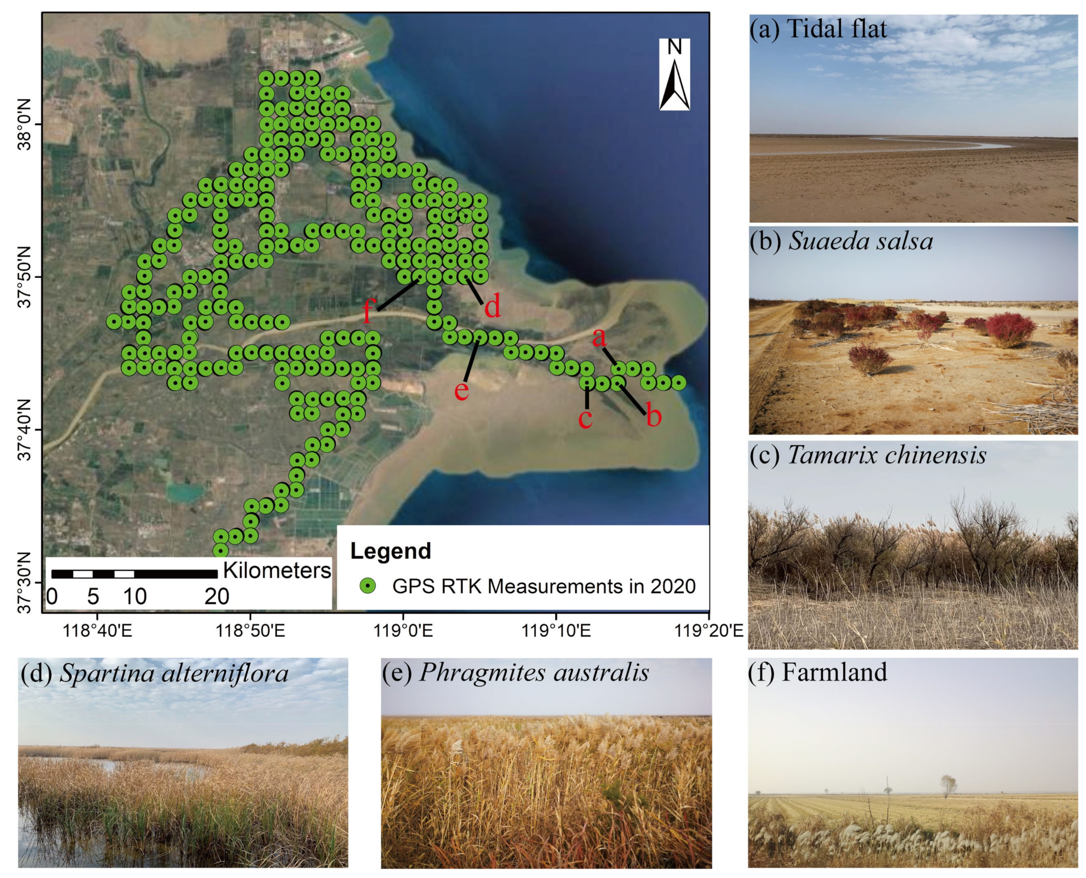
The Yellow River Delta (hereinafter referred to as YRD) has a complete range of estuarine wetland types, including salt marshes, mudflats, and tidal creeks [7,8]. However, intense anthropogenic activities in recent decades, such as dam building, agricultural irrigation, groundwater pumping, hydrocarbon extraction, and the artificial diversion of the estuary, have posed serious threats to the coastal wetlands of YRD [9,10,11,12,13]. Therefore, it is of great significance to carry out dynamic monitoring and obtain a reliable and up-to-date classification of coastal wetlands over the YRD for studying the impact of human activities on habitat area [14].
Wetland classification can illustrate the distribution and area of wetlands over geographical regions, which are helpful tools for evaluating the effectiveness of wetland policies [14]. In the last sixty years, wetland mapping and monitoring methods have been varied, mainly divided into field-based methods and remote sensing (RS) methods. Field-based wetland classification requires field work, which is labor-intensive, high in cost, time-consuming, and usually impractical due to poor accessibility. Therefore, it is only practical for relatively small areas [15]. In contrast, RS imagery can currently provide spatial coverage and repeatable observations in long-term series from local to regional scales, enabling effective detection and monitoring of different wetlands at a lower cost. However, wetland RS classification needs to be combined with sufficient field observations to train and evaluate the accuracy of classification [14]. RS has been demonstrated to be the most effective and economical method in wetland classification [15]. In addition, large-scale coastal wetland mapping is becoming a reality thanks to cloud computing platforms such as Google Earth Engine (GEE) [16,17].
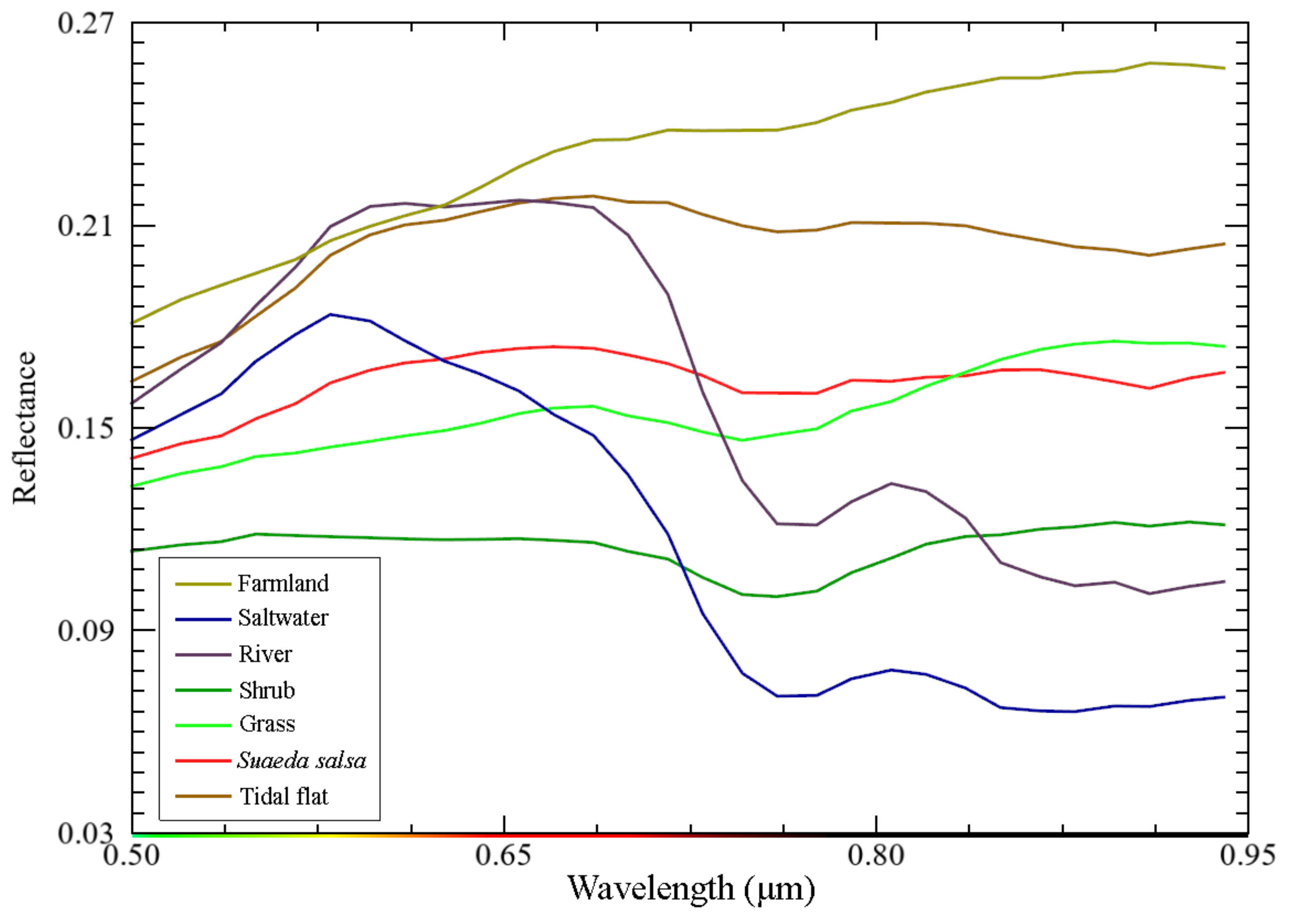
However, there are still some problems in the detection and classification of different types of wetland using satellite remote sensing images. The spectral curves of the same vegetation may be different due to the influence of growth environment, diseases, and insect pests. Additionally, two different vegetation may present the same spectral characteristics or mixed spectral phenomenon in a certain spectral segment, which makes it difficult to identify wetland types well by only using spectral response curves. These two phenomena greatly influence the classification algorithm based on spectral information and easily cause misclassification [18]. The particularity of wetlands makes wetland classification a challenging topic in remote sensing study.
Optical images can classify ground objects according to spectral features and various vegetation indices. Since the launch of the Landsat satellite in the late 1960s, wetland mapping has been an important application of remote sensing [19,20,21,22]. In the early stages, single data source and classical algorithms were mainly used, but now mapping has gradually started using multisource data fusion and complex algorithms [23]. With the launch of hyperspectral satellites, hyperspectral remote sensing images are gradually becoming widely used [24,25,26]. Hyperspectral data are sensitive to tiny spectral details and can detect resonance absorption and other spectral features of materials within the wavelength range of the sensor [27]. Melgani and Bruzzone [21] introduced support vector machines (SVM) to class hyperspectral images and proved that SVM is an effective alternative to conventional pattern recognition approaches (feature-reduction procedures combined with a classification method) to classify hyperspectral remote sensing data. Xi et al. [28] utilized Zhuhai-1 Constellation Orbita Hyperspectral Satellite (OHS) hyperspectral images for tree species mapping and indicated that hyperspectral imagery can efficiently improve the accuracy of tree species classification and has great application prospects for the future.
In recent years, the continuous launch of spaceborne synthetic aperture radar (SAR) systems have obtained a large number of on-orbit and historical archived data, providing an excellent opportunity for multi-temporal analysis, especially in coastal and cloudy areas [29]. Radar reflectivity is usually determined by the complex dielectric constant of the landcover, which in turn is dominated by the water content and geometric detail of the surface, e.g., smoothness or roughness of the surface and the adjacency of reflecting faces [27]. In the last two decades, many complicated and efficient classifiers and features have been investigated and integrated into the polarimetric SAR (hereinafter referred to as PolSAR) image classification framework to improve classification accuracy [30,31,32,33]. Li et al. [34] used Sentinel-1 dual polarization VV and VH data to discriminate treed and non-treed wetlands in boreal ecosystems. Mahdianpari et al. [35] use multi-temporal RADARSAT-2 fine resolution quad polarization (FQ) data to classify wetlands in Finland. The results show that the covariance matrix is a critical feature set of wetland mapping, and polarization and texture features can improve the overall accuracy. Therefore, the use of multi-temporal PolSAR classification shows considerable potential for wetland mapping. Full-polarization SAR data also have great advantages in wetland classification.
Previous studies have shown that multisensor remote sensing information fusion can improve the final quality of information extraction by relying on the existing sensor data without increasing the cost [23,36,37,38,39]. Due to the variety and complexity of coastal wetland types, it is necessary to consider multisource data fusion to improve the accuracy of wetland classification [7,40,41,42]. One approach is the synergetic classification of optical and SAR images, considered to be an effective way to improve the accuracy of ground object recognition and classification. For example, Li et al. [43] used GF-3 full-polarization SAR data and Sentinel-2 multispectral data to carry out synergetic classification of YRD wetlands, and the results were significantly superior to that of the single datum. Kpienbaareh et al. [44] used the dual polarization Sentinel-1, Sentinel-2, and PlanetScope optical data to map crop types. Niculescu et al. [45] identified an optimal combination of Sentinel-1, Sentinel-2, and Pleiades data using ground-reference data to accurately map wetland macrophytes in the Danube Delta, which suggests that diverse combinations of sensors are valuable for improving the overall classification accuracy of all of the communities of aquatic macrophytes, except Myriophyllum spicatum L. Thus, the fusion of available SAR and optical remote sensing data provides an opportunity for operational wetland mapping to support decisions such as environmental management.
However, a review of the existing literature yields few studies focused on the synergetic classification of coastal wetlands over the YRD, especially with GaoFen-3 (GF-3) full-polarization SAR and Zhuhai-1 OHS hyperspectral remote sensing in China. Therefore, in this study, we first introduce a combination method for coastal wetland classification over the YRD with both GF-3 and OHS images, and we then evaluate the classification accuracy. Furthermore, we investigate the influence of an optimal feature subset, seasonal change, and tidal height on the final classification.

2. Datasets and Methods

2.1. Study Area

As shown in Figure 1, the YRD is located in the northeast of Shandong province, China, and is bounded by the Bohai Sea to the north and Laizhou Bay to the east [12,39]. It is a fan-shaped area formed by sedimentation of the Yellow River as it flows into the Bohai Sea, where newly formed wetlands are increasing at a rate of 30 km2 per year. The terrain of the region is flat, with diverse types and complex geomorphic forms and an average slope of 2.14% [10,36,39,46]. Tidal creeks are widely distributed in the coastal areas on the north and south sides of the YRD. This region is in the temperate monsoon climate zone, with an average annual temperature of 14.7 °C and average precipitation of approximately 526 mm/year during January 2019 and December 2020 [7].
The YRD wetland is a typical estuarine wetland ecosystem of salt marsh, which belongs to the coastal wetland classified by the Ramsar Wetland Convention [47,48]. The total area of wetland in the YRD is approximately 700 km2, of which the area of natural wetland accounts for approximately 89%, mainly including shallow sea, tidal flat, river, and vegetation, and the area of human-made wetland accounts for approximately 11%, mainly including aquaculture ponds, salt pans, and farmland. Four dominant salt marsh plant species, namely, Phragmites australis, Tamarix chinensis, Spartina alterniflora, and Suaeda salsa, occupy the broad tidal flats of the YRD [20,37]. Suaeda salsa and Tamarix chinensis are the only halophytic plants in heavy saline soil and tidal flats. When the soil is desalted, the vegetation type changes to Phragmites australis.

2.2. Datasets

2.2.1. GF-3 and OHS

The Chinese Gaofen-3 (GF-3) satellite carried a SAR sensor and was launched on 10 August 2016 [30]. The GF-3 supports operations in single-polarization (HH or VV), dual-polarization (HH+HV or VH+VV), and quad-polarization (HH+HV+VH+VV) modes with respect to 12 different observing modes [49], and has been widely used for water conservancy, land and ocean monitoring, and other vital applications [50,51].
QPSI is a quad-polarization strip imaging mode with a spatial resolution of 8 m that captures four polarization channels by transmitting and receiving horizontal and vertical waves and can improve the classification accuracy of ground targets [33]. The detailed parameters of GF-3 data selected for this study are shown in Table 1.
The Zhuhai-1 satellite constellation of Orbita company includes four Orbita hyperspectral satellites (OHS-A, OHS-B, OHS-C, and OHS-D) that have the same hardware configuration and operating status as well as strong hyperspectral data acquisition abilities [52]. The hyperspectral sensor CMOSMSS (Complementary Metal-Oxide-Semiconductor Multispectral Scanner System) mounted on the OHS satellites can acquire images with a resolution of 10 m, a width of 150 km, and 32 spectral segments [53]. The detailed parameters and spectral range of the OHS bands used for this study are shown in Table 1 and Table 2.

2.2.2. Training and Validation Samples

The quality of samples is directly related to the accuracy of wetland information extraction, so pure typical and representative pixels should be selected as samples. The training and validation samples in this study are mainly derived from two methods: field survey and visual interpretation with Google Earth high-resolution optical remote sensing images, as well as GaoFen-2 (GF-2) panchromatic and multispectral fusion images with nadir pixel resolution of 0.8 m. In November 2020, our research group conducted a detailed field survey of the YRD National Nature Reserve, using Global Position System real time kinematic (GPS RTK) measurements to locate, record, and take photos of different wetland distributions and wetland types, as shown in Figure 2. The above two categories of data constitute sample data and validation data, which are used to establish classifiers and verify accuracy. Table 3 lists the per-class numbers for the classification training and validation samples (a total of 219,269 samples).
According to the investigation of wetlands in the YRD, the main wetland types in the wetland are Tamarix chinensis, Suaeda salsa, Phragmites australis, and invasive species Spartina alterniflora [7,37,41].
  • Tamarix chinensis is a kind of tree or shrub with a height of 3–6 m. It is popular on river alluvial plain, seashore, beachhead, wet saline land, and sandy wasteland.
  • Suaeda salsa is an annual herb that grows up to 1 m tall, growing in the seashore, wasteland, ditch shore, the edge of the field, and other saline soil.
  • Phragmites australis (commonly known as reed) is a tall aquatic or wet perennial grass, up to 1–3 m tall. It does not grow in forest habitats but in various open waterborne areas, such as rivers, lakes, ponds, watercourses, and lowland wetlands.
  • Spartina alterniflora grows best on muddy beaches in estuaries. In the YRD, Spartina alterniflora usually grows in the intertidal zone of estuaries, bays, and other coastal tidal flats with elevations from 0.7 m below the mean sea level to the mean high-water level and forms a dense single-species community.
As shown in Figure 2, a field survey of the YRD wetland was conducted from 9 November 2020 to 13 November 2020. Due to the similar morphological and spectral characteristics as well as lack of prior knowledge, Phragmites australis and Spartina alterniflora were merged into the group of grass, whereas shrub was used to represent the Tamarix chinensis. Therefore, the wetlands in the YRD is divided into seven types: saltwater, farmland, river, shrub, grass, Suaeda salsa, and tidal flat.

2.3. Methods

Figure 3 presents the overall technical flow chart of this study, including data preprocessing, features extraction, datasets fusion, supervised classification, and accuracy evaluation. The detailed data processing process is shown below.

2.3.1. GF-3 Preprocessing

As shown in Figure 3, GF-3 PolSAR image processing consists of image preprocessing, features extraction, image classification, and accuracy evaluation.
First, the preprocessing of the original PolSAR image in single look complex (SLC) format was performed with Pixel Information Expert SAR (PIE-SAR®) 6.0 and ENVI® 5.6, including radiometric calibration, polarization filtering, and polarization matrix conversion. After importing the GF-3 full-polarization SAR data, the radiometric correction process can be completed automatically. A polarized scattering matrix can only describe so-called coherent or pure scatterers, whereas distributed scatterers usually use second-order descriptors [54]. Therefore, after importing the data, the polarization scattering matrix was converted into the polarization covariance matrix or polarization coherence matrix by means of a transformation function. PolSAR image speckle noise seriously affects the image quality, accuracy of landcover information extraction, and ground object interpretation. Azimuth and range multi-looking of 3*3 and the refined Lee filter with the window size of 3 × 3 were employed to reduce speckle noise with the output image grid size of 8 m.
Feature extraction is divided into two steps. The first step is polarization decomposition, which aims to effectively separate ground objects dominated by different scattering mechanisms. Polarization features derived from polarization decomposition can reveal the scattering mechanism of the ground object to determine the type. For example, surface scattering is dominant in water bodies, whereas secondary scattering and volume scattering are dominant in residential land and forest, respectively. The polarization decomposition was carried by the H-A-α decomposition method and the three-component Freeman decomposition method, respectively [23].
H-A-α decomposition uses the scattering matrix transformation to obtain the coherency matrix [T3], where [T3] is a semi-positive definite Hermite matrix [31]. The three second-order parameters of H-A-α decomposition are the eigenvalues and eigenvector functions of [T3], which are defined as follows [32]:
  • entropy H:
    H = k = 1 3 P k log 3 ( P k )
In the formula, P i = λ i / k = 1 3 λ k , k = 1 3 P i = 1 . Entropy H reflects the randomness of the target scattering mechanism. For example, a low H indicates that only one scattering mechanism is dominant, whereas a high H indicates more than two primary scattering mechanisms.
  • alpha α:
    α = P 1 α 1 + P 2 α 2 + P 3 α 3
In the formula, the magnitude of α1, α2,and α3 indicates the primary scattering mechanism: surface scattering, secondary scattering, and volume scattering; α denotes the scattering angle. When α is close to 0, it indicates that only one scattering mechanism exists. In contrast, a larger α value (maximum 90 degrees) indicates a more complex surface scattering mechanism.
  • anisotropy A:
    A = λ 2 λ 3 λ 2 + λ 3
In the formula, λi is the eigenvalue of the coherency matrix [T3]. Anisotropy reflects the relationship between two smaller scattering mechanisms. High A represents that two scattering mechanisms are dominant simultaneously, whereas low values of A and H show that only one scattering mechanism is dominant. However, low A and high H indicate that three scattering mechanisms are similar, and the scattering is almost random.
Therefore, the polarization scattering information of ground objects can be fully used to distinguish the surface types effectively. Figure 4 roughly shows the general distribution of wetlands in the YRD. The low entropy value of water bodies such as oceans and rivers indicates that surface scattering is dominant, whereas the high entropy value and low anisotropy of land show a mixture of two or more scattering mechanisms (Figure 4b,c). The estuarine and riverside areas appear red (Figure 4a), mainly due to the volume scattering of vegetation.
The Freeman three-component decomposition based on the physical reality was used to establish a polarization covariance matrix with three basic scattering mechanism models, namely, surface scattering, P S ; volume scattering, P V ; and secondary scattering, P D . The total polarization power was then solved using the above three scattering components, and the formula is as follows [23,54]:
P S P A N = S H H 2 + 2 S H V 2 + S V V 2 = P S + P D + P V
The second step is to extract texture features from the total polarization power by using gray level co-occurrence matrix (GLCM) and generate eight features, namely, mean, variance, homogeneity, contrast, dissimilarity, entropy, angular second moment, and correlation [55]. Correlation can quantify the directionality of terrain texture. In addition, variance, dissimilarity, and contrast can be used to analyze texture periodicity, whereas entropy, angular second moment, and homogeneity can represent texture complexity [56].
M e a n x = x y P S P A N x , y x M e a n y = x y P S P A N x , y y
V a r i a n c e x = x y P S P A N x , y x M e a n x 2 V a r i a n c e y = x y P S P A N x , y y M e a n y 2
H o m o g e n e i t y = x y P S P A N x , y 1 + x y 2 , x y
C o n t r a s t = x y x y 2 P S P A N x , y
D i s s i m i l a r i t y = x y P S P A N x , y x y
E n t r o p y = - x y P S P A N x , y log P S P A N x , y
E n e r g y ( a n g u l a r   s e c o n d   m o m e n t ) = x y P S P A N 2 x , y
C o r r e l a t i o n = x y x , y P S P A N x , y M e a n x M e a n y V a r i a n c e x V a r i a n c e y
As shown in Figure 5, a false color image with three texture features can be used to display the surface texture information, river extension, and tidal creek development in the YRD. Red land and blue water indicate that the land surface is rough and ground types vary with obvious texture, whereas the texture difference of the water area is slight. Due to the significant morphological differences between estuarine and riverside vegetations, such as Phragmites australis and Tamarix chinensis, the texture changes rapidly.

2.3.2. OHS Preprocessing

The procedure of OHS data preprocessing with the hyperspectral image processing software PIE-Hyp® 6.0 and ENVI® 5.6 is shown in Figure 3. There are 32 bands in the original OHS hyperspectral data [52]. First, all the bands were tested to identify any bad bands. Bands with no data or poor quality were marked as bad. If there was a bad band, it needed to be repaired. Radiation calibration [57] and atmospheric correction [58] were then carried out for the above bands, respectively.
Hyperspectral images have rich spectral features, which can be combined with their derived features to carry out fine wetland classification. As shown in Figure 6, spectral values of different wetland types in OHS hyperspectral images were plotted according to the region of interest (ROI) of the training samples. The spectral curves of seven wetland types are relatively low, with the highest spectral reflectance of farmland and tidal flat and the lowest spectral reflectance of saltwater. The spectral reflectance curves of saltwater and river are similar with an absorption peak in the near-infrared band, but the spectral reflectance of the river is slightly higher than that of saltwater on the whole. Additionally, the spectral reflectance curves of shrub and grass are also similar, but the overall reflectance of grass is higher than that of the shrub. There is no obvious difference in spectral reflectance between Suaeda salsa and grass, especially in the near-infrared band, resulting in a low separability between the two types of wetlands. In conclusion, the spectral reflectance separability of the seven wetland types is not very significant, which would lead to classification errors of some wetlands and affect the accuracy of classification results to a certain extent.
Previous studies have shown that the Hughes phenomenon exists in the classification process due to a large number of hyperspectral bands [59]. Feature extraction, also known as dimensionality reduction, can not only compress the amount of data, but also improve the separability between different categories of features to obtain the optimal features, which is conducive to accurate and rapid classification [60].
The classification of remote sensing images is mainly based on the spectral feature of pixels and their derived features. In this study, principal component analysis (PCA) was used as the spectral feature extraction algorithm to obtain the first five bands, whose eigenvalues were much larger than those of other bands [61]. As one of the most widely used data dimension reduction algorithms, PCA is defined as an optimal orthogonal linear transformation with minimum mean square error established on statistical characteristics [24]. By transforming the data into a new coordinate system, the greatest variance by some scalar projection of the data comes to lie on the first coordinate, which is called the first principal component, the second greatest variance on the second coordinate, etc. In addition to spectral features, we also employed normalized difference vegetation index (NDVI) [62] and normalized difference water index (NDWI) [63] to obtain index features. The formulas of NDVI and NDWI are as follows.
N D V I = ( N I R R e d ) ( N I R + R e d ) = B 24 B 14 B 24 + B 14
N D W I = ( G r e e n N I R ) ( G r e e n + N I R ) = B 7 B 23 B 7 + B 23
where NIR, Red, and Green represent the near-infrared band, red band, and green band, respectively.
As shown in Table 3, band 24 and band 14 from the OHS data are selected for NDVI, whereas band 7 and band 23 are suitable for NDWI. Figure 7 presents the two kinds of OHS hyperspectral index features. Both the NDVI value for land and NDWI value for water are positive, which can basically represent the spatial distribution of land vegetation and water.

2.3.3. Synergetic Classification

GF-3 polarization and texture features (8 m) and OHS spectral and index features (10 m) derived from the above steps were used to carry out synergetic classification. Before classification, the spatial resolution of the two kinds of data should be consistent through resampling, which was set to 10 m in this study.
After ortho-rectification and image coregistration, the above features were classified through three classical supervised classification methods, including maximum likelihood (ML) [25], Mahalanobis distance (MD) [26], and support vector machine (SVM) [21]. In this study, to obtain the fusion datasets of GF-3 PolSAR and OHS hyperspectral data for coastal wetland classification, the layer stacking method was used to combine 11 GF-3-derived polarization and texture features and seven OHS derived spectral and index features into one multiband image at the feature level. This new multiband image includes a total of 18 bands.
The classifiers represent three different classification principles, as shown below.
  • The ML classifier is one of the most popular methods of classification in remote sensing, in which a pixel with the maximum likelihood is classified into the corresponding class. The likelihood Lk is defined as the posterior probability of a pixel belonging to class k.
    L ω i = p ω i x = p x ω i p ω i p x = p x ω i p ω i i = 1 M p x ω i p ω i
    where p(ωi) and p(x|ωi) are the prior probability of class ωi and the conditional probability density function to observe x from class ωi, respectively. Usually, p(ωi) is assumed to be equal, and p(x|ωi)p(ωi) is also common to all classes. Therefore, i depends on the probability density function p(x|ωi).
  • The MD classifier is a direction-sensitive distance classifier that uses statistics for each class. It is similar to the ML classifier, but it assumes that all classes have equal covariances, and is, therefore, less time-consuming. The MD of an observation x = (x1, x2, x3, …, xn)T from a set of observations with mean μ = (μ1, μ2, μ3,…, μn)T and covariance matrix S is defined as [26]:
    D M x = = x μ T S 1 x μ
  • The SVM classifier is a supervised classification method that often yields good classification results from complex and noisy data. It is derived from statistical learning theory that separates the classes with a decision surface that maximizes the margin between the classes. The surface is often called the optimal hyperplane, and the data points closest to the hyperplane are called support vectors. If the training data are linearly separable, any hyperplane can be written as the set of points x satisfying:
    w T x b = 0
    where w is the normal vector to the hyperplane.
The labeled training samples were used as input, and the classification results of seven wetland types were obtained by using the above classifiers to predict the class labels of test images.

2.3.4. Accuracy Assessment

As the most standard method for remote sensing image classification accuracy, the confusion matrix (also called error matrix) was employed to quantify misclassification results. The accuracy metrics derived from the confusion matrix include overall accuracy (OA), Kappa coefficient, user’s accuracy (UA), producer’s accuracy (PA), and F1-score [64]. The number of validation samples per class used to evaluate classification accuracy is shown in Table 3. A total of 98,009 samples were applied to assess the classification accuracies.
The OA describes the proportion of correctly classified pixels, with 85% being the threshold for good classification results. The UA is the accuracy from a map user’s view, which is equal to the percentage of all classification results that are correct. The PA is the probability that the classifier has labeled a pixel as class B given that the actual (reference data) class is B and is an indication of classifier performance. The F1-score is the harmonic mean of the UA and PA and gives a better measure of the incorrectly classified cases than the UA and PA. The Kappa coefficient is the ratio of agreement between the classification results and the validation samples, and the formula is shown as follows [22].
K a p p a   c o e f f i c i e n t = N i = 1 r X i i i = 1 r X i + X + i N 2 i = 1 r X i + X + i
where r represents the total number of the rows in the confusion matrix, N is the total number of samples, X i i is on the i diagonal of the confusion matrix, X i + is the total number of observations in the i row, and X + i is the total number of observations in the i column.

3. Results

The classification results derived from the ML, MD, and SVM methods for the GF-3, OHS, and synergetic data sets in the YRD are presented in Figure 8. First, a larger amount of noise deteriorates the quality of GF-3 classification results, and many pixels belonging to the river are misclassified as saltwater (Figure 8a,d,g), indicating that the GF-3 fails to separate different water bodies (e.g., river and saltwater). Second, the OHS classification results (Figure 8b,e,h) are more consistent with the actual distribution of wetland types, proving the spectral superiority of OHS. However, there are many river noises in the sea that are probably attributed to the high sediment concentrations in shallow sea areas (see Figure 1). Third, the complete classification results generated by the synergetic classification are clearer than those of GF-3 and OHS data separately (Figure 8c,f,i). Similarly, some unreasonable distributions of wetland classes in the OHS classification also exist in the synergetic classification results, which reduces the classification performance. For example, river pixels appear in the saltwater, and Suaeda salsa and tidal flat exhibit unreasonable mixing. Overall, the ML and SVM methods can produce a more accurate full classification that is closer to the real distribution.
The accuracy results obtained by different classification methods for different data sets are shown in Table 4, Table 5, Table 6, and Table 7, and Figure 9, Figure 10, and Figure 11. The OAs obtained by the ML, MD, and SVM methods for the GF-3 data are 52.5%, 55.7%, and 80.7%, and the Kappa coefficients are 0.36, 0.41, and 0.70, respectively. The above classification accuracy is the lowest of all classification processes, possibly due to common wetland structural conditions. In contrast, the OAs with the ML, MD, and SVM methods for the OHS data are 96.7%, 87.6%, and 95.6%, and the Kappa coefficients are 0.95, 0.82, and 0.94, respectively. This may be attributed to the increased spectral separation capacity of the biochemical characteristics of wetland types. Subsequently, the classification accuracy after data fusion is improved by approximately 30% compared with the GF-3 data alone. This is mainly due to the consideration of the biophysical and biochemical changes that occur with the change in the phenology of wetland types.
Considering that the synergetic technique essentially combines the structural and dielectric information of wetland types with the scattered power components, GF-3 and OHS data are transformed into more meaningful target information content than the GF-3 or OHS data alone. Therefore, we found that the accuracy metrics of synergetic classification were significantly improved compared with the single data classification in Table 4 and Figure 9. Among the three tested classifiers, the MD method provides the lowest synergetic classification accuracy of 89%, and the other two methods (ML and SVM) are relatively close, with an overall accuracy of 97% and a Kappa coefficient of 0.96.
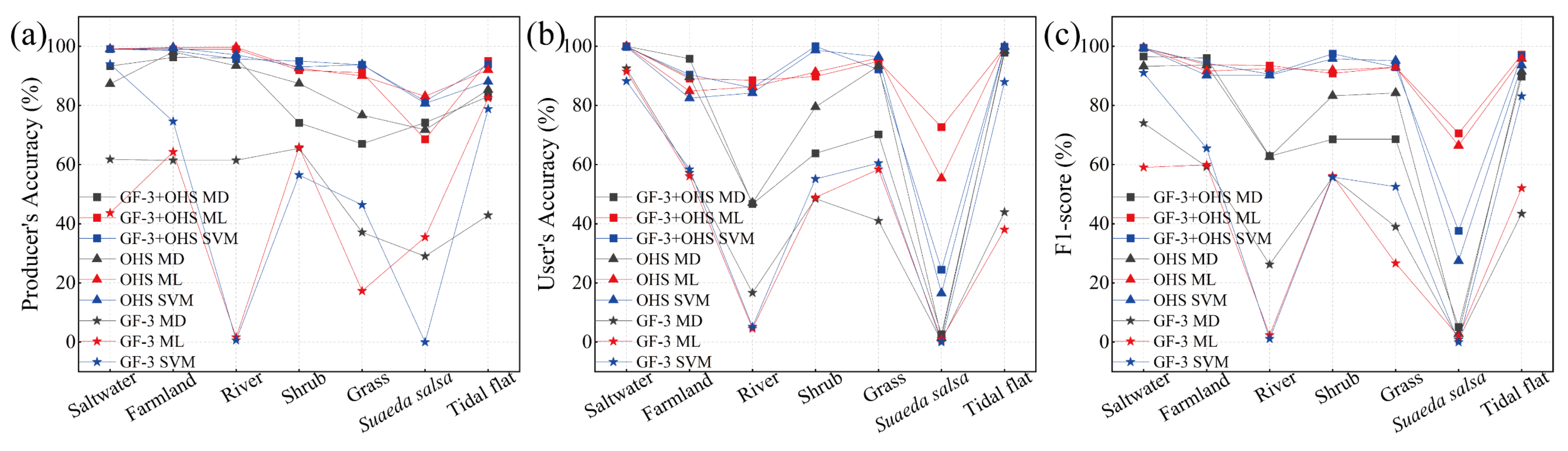
In addition to the OA and Kappa coefficients (Table 4 and Figure 9) and corresponding classification images (Figure 8), the PA, UA, and F1-score were calculated according to the confusion matrix (Table 5, Table 6 and Table 7 and Figure 10). Concerning the values of PA, UA, and F1-score obtained for each wetland type, the best classified types are saltwater, farmland, river, and tidal flat, with values above 80%. The accuracy of Suaeda salsa was the lowest, mainly due to the fact that Suaeda salsa is small in size (approximately 1 m in height and width) and sparsely distributed on the tidal flat, whereas the image resolution of 10 m was used in this study. The PA, UA, and F1-score of saltwater and river for GF-3 data are significantly lower than those of the other two datasets. Since SAR distinguishes objects by different scattering mechanisms and surface roughness, the above two factors are basically the same in saltwater and river, making it difficult to distinguish between them. Therefore, the spectral characteristics of optical images are required to improve the PA, UA, and F1 scores of water bodies.
For synergetic classification, the PA, UA, and F1-score are above 90% as most phenological features are captured by the SAR backscatter coefficients and OHS spectral information. Although there is an overall increase in the Kappa coefficient, OA, UA, PA, and F1-score for different wetlands with synergetic classification, the PA, UA, and F1-score of shrub, grass, and Suaeda salsa are abnormal, respectively. The decrease in the UA, PA, and F1-score could be due to the fact that the sample pixels used for training are insufficient. Considering the complexity of wetlands in the study areas, these levels of accuracy prove the robustness and high performance of the proposed synergetic classification in different study areas with various ecological characteristics.
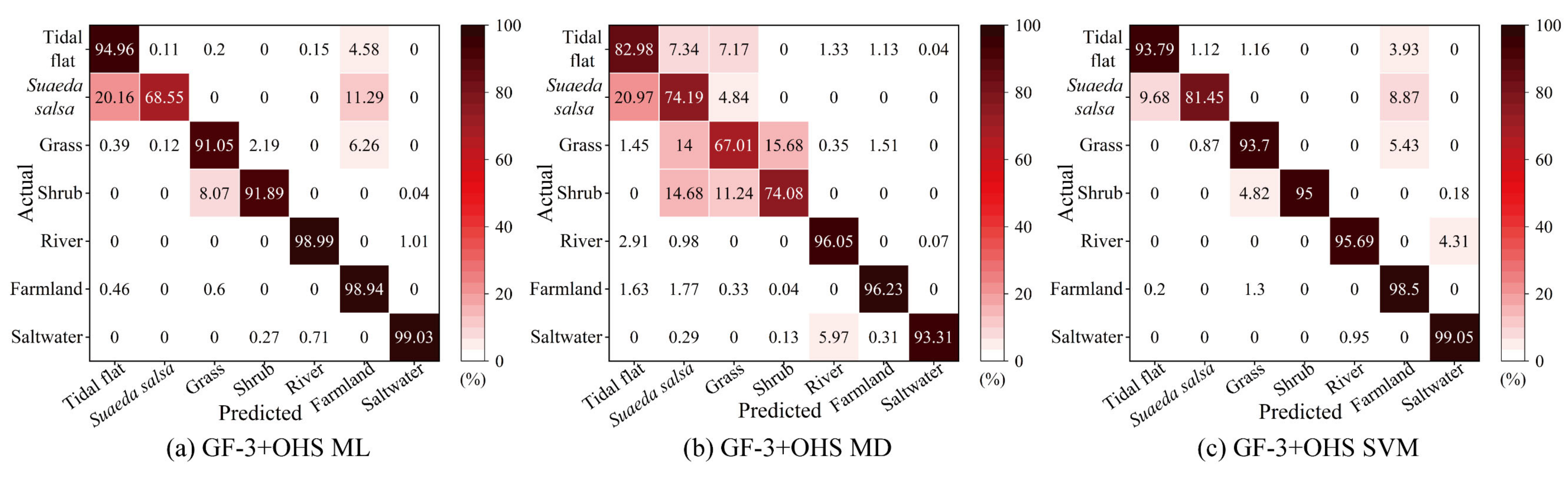
Misclassification commonly occurs in the process of image classification. The fewer misclassified categories and misclassified pixels, the better the results of the classification. Figure 11 is a graphical representation of the confusion matrix. Most off-diagonal cells have low values, indicating that most pixels are reasonably well classified. In particular, the results of the ML synergetic classification show that part of the tidal flats were wrongly classified as Suaeda salsa, grass, river, and farmland. In a few cases, saltwater was also misclassified as shrub and river. The biggest omission was the misclassification of Suaeda salsa as tidal flat and farmland. In general, there is extensive confusion between adjacent succession groups, such as saltwater vs. river, farmland vs. tidal flat, and shrub vs. grass.

4. Discussion

4.1. Significance Analysis of Multi-Features

Hyperspectral remote sensing images have rich spectral information, which is the main basis of image classification. In contrast, SAR images can record geometric and physical properties, such as surface roughness and dielectric constant through backscattering intensity. The PolSAR image features that can be used for classification include polarization features and texture features. The unique spatial information of these features can effectively supplement the hyperspectral image information, which has proven to be beneficial to the fine classification of ground objects.
The ranking of the importance of all the GF-3 and OHS features by the Recursive Feature Elimination (RFE) [65] method is shown in Figure 12a, which is used to represent the separate contributions to the final synergetic classification. There are seven most important features, namely, entropy (T), contrast, anisotropy, correlation, homogeneity, energy, and NDWI. However, we found that the final overall accuracy and Kappa coefficient derived from all 18 features are higher than those from the seven most important features, as shown in Figure 12b.
Figure 13 shows box-and-whisker diagrams for the seven most important features, which provide a preliminary insight into the causes of misclassification. It can be seen that these seven features can better distinguish the wetland landcover types. The features, such as entropy, anisotropy, homogeneity, and NDWI, contribute greatly to distinguishing different landcover due to the spectrum and appearances of wetland (Figure 13a,c,e,g). However, contrast and correlation features do not perform well due to similar wetland texture features (Figure 13b,d). The low separability of some wetland types, e.g., saltwater vs. river, farmland vs. tidal flat, and shrub vs. grass, gives rise to misclassification to a great extent.

4.2. Influence of Seasonal Change

For multi-source satellite remote sensing images obtained in different seasons, the phenological differences cause false changes, which make the synergetic classification of wetlands very challenging [38]. Images taken at different times show different types of land types and different vegetation growth states. Therefore, when multi-source data are fused, images observed in the same season should be used; otherwise, the reliability of synergetic classification may be affected [38,66].
The YRD is located in the warm temperate zone with four distinct seasons and large seasonal variations in land cover [67]. The GF-3 and OHS remote sensing images in this study were collected on 13 March2019, and 23 March 2020, respectively. As shown in Figure 14, the highest temperature in March in this region was 17 °C, the lowest temperature was 2 °C, and the highest precipitation was 4 mm. Most plants were not in the vigorous growth stage, and the change rate of land cover was relatively low. In addition, the study area is located in the YRD National Nature Reserve with relatively little human disturbance. In recent years, the impact of sediment transport on the Yellow River estuary has gradually decreased [39]. Therefore, the images collected in the same month in this study can ensure the maximum reduction in the impact of wetland phenological changes.

4.3. Influence of Tidal Level

Because the wetlands in the tidal flats over the YRD are greatly affected by tides, the effect of tidal height on synergetic classification accuracy should be considered when using multi-source images to classify coastal wetlands.
Combined with the tidal data of Dongying Port, the tidal heights are 103 cm and 106 cm of SAR and hyperspectral, respectively, and the tidal difference between SAR and hyperspectral image acquisition time is approximately 3 cm. The OHS image in 2020 corresponds to saltwater, but the GF-3 image in 2019 corresponds to tidal flat. According to the Advanced Land Observing Satellite World 3D-30m (AW3D30) v3.2, the average slope of the estuary is estimated at 2.14%. A tidal difference of 3 cm corresponds to a horizontal change of nearly 70 m along the coastline. As the spatial resolution of the classification is 10 m, 70 m corresponds to 7 pixels. Therefore, the difference in tide level could introduce uncertainty in the classification results.

4.4. Comparison with Other Studies

In this study, a synergetic wetland classification method combining GF-3 full-polarization SAR and OHS hyperspectral images is proposed to generate a high-accuracy and reliable wetland classification of the YRD. The OAs obtained by the ML, MD, and SVM methods for the synergetic data sets are 97.3%, 89.0%, and 97.2%, and the Kappa coefficients are 0.96, 0.84, and 0.96, respectively. Compared with the single data set, the synergetic classification method combined with OHS and GF-3 can further improve the accuracy and meet the demand of a high-accuracy wetland classification in the YRD, which has great potential in other wetland classification scenarios.
Previous studies have provided a number of synergetic classification cases for multi-source SAR and optical remote sensing data integration, such as Sentinel-1, Sentinel-2, and PlanetScope, to generate high-precision land cover and wetland classification results, regardless of seasonal variations and tidal effects [23,40,42,44,45]. For example, Slagter et al. [40] used Sentinel-1 and Sentinel-2 data to provide a more detailed spatial distribution of the St. Lucia wetland habitats without considering wetland dynamics. Cai et al. [42] demonstrated the good performance of the object-based stacked generalization method by combining multitemporal optical and SAR data, with an overall accuracy of 92.4% and a Kappa coefficient of 0.92, respectively. Nevertheless, some prediction errors may exist in the low-resolution prior images if the temporal land surface changes are too indiscernible.
Some scholars have conducted preliminary studies on the classification of coastal wetlands in the YRD without using full-polarization SAR data or hyperspectral data. In particular, there are few synergetic wetland classification studies that evaluate the GF-3 and OHS data. For example, Feng et al. [36] proposed a multibranch convolutional neural network (MBCNN) to fuse Sentinel-1 and Sentinel-2 images to map YRD coastal land cover, with an overall accuracy of 93.8% and a Kappa coefficient of 0.93. Zhang et al. [7] mapped the distribution of salt marsh species with the integration of Sentinel-1 and Sentinel-2 images. However, only the Sentinel-2 vegetation index and Sentinel-1 backscattering feature are used, but the polarization feature of SAR images is not fully utilized.

5. Conclusions

Wetland classification is a challenging task for remote sensing research due to the similarity of different wetland types in spectrum and texture, but this challenge could be eased by the use of multi-source satellite data. In this study, a synergetic classification method for GF-3 full-polarization SAR and OHS hyperspectral imagery was proposed in order to offer an updated and reliable spatial distribution map for the entire YRD coastal wetland. Three classical machine learning algorithms (ML, MD, and SVM) were used for the synergetic classification of 18 spectral, index, polarization, and texture features. According to the field investigation and visual interpretation, the overall synergetic classification accuracy of 97% for ML and SVM algorithms is higher than that of single GF-3 or OHS classification, which proves the performance of the fusion of fully polarized SAR data and hyperspectral data in wetland mapping.
The spatial distribution of coastal wetlands affects their ecological functions. Detailed and reliable wetland classification can provide important wetland type information to better understand the habitat range of species, migration corridors, and the consequences of habitat change caused by natural and anthropogenic disturbances. The synergy of PolSAR and hyperspectral imagery enables high-resolution classification of wetlands by capturing images throughout the year, regardless of cloud cover. Therefore, the proposed method has the potential to provide accurate results in different regions.

Author Contributions

Conceptualization, P.L. and Z.L.; methodology, C.T., P.L., D.L., and Z.L.; formal analysis and validation, C.T., D.L., and P.L.; investigation, C.T., P.L., D.L., Q.Z., M.C., J.L., G.W., and H.W.; resources, P.L., S.Y., and Z.L.; writing—original draft preparation, C.T. and P.L.; writing—review and editing, C.T., P.L., Z.L., H.W., M.C., and Q.Z.; project administration, P.L., Z.L., and H.W.; data curation, C.T., S.Y., and P. L.; visualization, C.T. and P. L.; supervision, P.L., Z.L., and H.W.; funding acquisition, P.L., Z.L., and H.W. All authors have read and agreed to the published version of the manuscript.

Funding

This work was jointly supported by the Natural Science Foundation of China (no. 42041005-4; no. 41806108), National Key Research and Development Program of China (no. 2017YFE0133500; no. 2016YFA0600903), Open Research Fund of State Key Laboratory of Estuarine and Coastal Research (no. SKLEC-KF202002) from East China Normal University, as well as State Key Laboratory of Geodesy and Earth’s Dynamics from Innovation Academy for Precision Measurement Science and Technology, Chinese Academy of Sciences (SKLGED2021-5-2). Z.H. Li was supported by the European Space Agency through the ESA-MOST DRAGON-5 Project (ref.: 59339).

Acknowledgments

The authors are grateful to colleagues from the Ocean University of China for conducting the field GPS RTK measurements in the Yellow River Delta. ERA5 data are freely available from the Copernicus Climate Change Service (C3S). Tide level data are provided by the National Marine Data and Information Service (NMDIS), China. The authors thank the National Satellite Ocean Application Service for providing the GF-2 and GF-3 data. We also thank the Zhuhai Orbita Aerospace Science & Technology Co. Ltd. for providing the Zhuhai-1 OHS data. Finally, the authors sincerely thank all anonymous reviewers and the editors for their constructive and excellent reviews that have greatly improved the quality of the article.

Conflicts of Interest

The authors declare no conflict of interest.

References

  1. Schuerch, M.; Spencer, T.; Temmerman, S.; Kirwan, M.L.; Wolff, C.; Lincke, D.; McOwen, C.J.; Pickering, M.D.; Reef, R.; Vafeidis, A.T.; et al. Future response of global coastal wetlands to sea-level rise. Nature 2018, 561, 231–234. [Google Scholar] [CrossRef] [PubMed]
  2. Bonan, G.B. Forests and Climate Change: Forcings, Feedbacks, and the Climate Benefits of Forests. Science 2008, 320, 1444. [Google Scholar] [CrossRef] [PubMed] [Green Version]
  3. Wang, F.; Lu, X.; Sanders, C.J.; Tang, J. Tidal wetland resilience to sea level rise increases their carbon sequestration capacity in United States. Nat. Commun. 2019, 10, 5434. [Google Scholar] [CrossRef]
  4. Lin, W.-J.; Wu, J.; Lin, H.-J. Contribution of unvegetated tidal flats to coastal carbon flux. Glob. Chang. Biol. 2020, 26, 3443–3454. [Google Scholar] [CrossRef]
  5. Wang, F.; Sanders, C.J.; Santos, I.R.; Tang, J.; Schurech, M.; Kirwan, M.L.; Kopp, R.E.; Zhu, K.; Li, X.; Yuan, J.; et al. Global blue carbon accumulation in tidal wetlands increases with climate change. Natl. Sci. Rev. 2020, 8, nwaa296. [Google Scholar] [CrossRef]
  6. Wang, F.; Tang, J.; Ye, S.; Liu, J. Blue Carbon Sink Function of Chinese Coastal Wetlands and Carbon Neutrality Strategy. Bull. Chin. Acad. Sci. 2021, 36, 1–11. [Google Scholar] [CrossRef]
  7. Zhang, C.; Gong, Z.; Qiu, H.; Zhang, Y.; Zhou, D. Mapping typical salt-marsh species in the Yellow River Delta wetland supported by temporal-spatial-spectral multidimensional features. Sci. Total Environ. 2021, 783, 147061. [Google Scholar] [CrossRef]
  8. Su, H.; Yao, W.; Wu, Z.; Zheng, P.; Du, Q. Kernel low-rank representation with elastic net for China coastal wetland land cover classification using GF-5 hyperspectral imagery. ISPRS J. Photogramm. Remote Sens. 2021, 171, 238–252. [Google Scholar] [CrossRef]
  9. Lin, Q.; Yu, S. Losses of natural coastal wetlands by land conversion and ecological degradation in the urbanizing Chinese coast. Sci. Rep. 2018, 8, 15046. [Google Scholar] [CrossRef]
  10. Wu, X.; Bi, N.; Xu, J.; Nittrouer, J.A.; Yang, Z.; Saito, Y.; Wang, H. Stepwise morphological evolution of the active Yellow River (Huanghe) delta lobe (1976–2013): Dominant roles of riverine discharge and sediment grain size. Geomorphology 2017, 292, 115–127. [Google Scholar] [CrossRef]
  11. Kirwan, M.L.; Megonigal, J.P. Tidal wetland stability in the face of human impacts and sea-level rise. Nature 2013, 504, 53–60. [Google Scholar] [CrossRef] [PubMed]
  12. Wang, G.; Li, P.; Li, Z.; Ding, D.; Qiao, L.; Xu, J.; Li, G.; Wang, H. Coastal Dam Inundation Assessment for the Yellow River Delta: Measurements, Analysis and Scenario. Remote Sens. 2020, 12, 3658. [Google Scholar] [CrossRef]
  13. Syvitski, J.P.M.; Kettner, A.J.; Overeem, I.; Hutton, E.W.H.; Hannon, M.T.; Brakenridge, G.R.; Day, J.; Vörösmarty, C.; Saito, Y.; Giosan, L.; et al. Sinking deltas due to human activities. Nat. Geosci. 2009, 2, 681–686. [Google Scholar] [CrossRef]
  14. Mahdavi, S.; Salehi, B.; Granger, J.; Amani, M.; Brisco, B.; Huang, W. Remote sensing for wetland classification: A comprehensive review. GIScience Remote Sens. 2018, 55, 623–658. [Google Scholar] [CrossRef]
  15. Schmidt, K.S.; Skidmore, A.K. Spectral discrimination of vegetation types in a coastal wetland. Remote Sens. Environ. 2003, 85, 92–108. [Google Scholar] [CrossRef]
  16. Sun, S.; Zhang, Y.; Song, Z.; Chen, B.; Zhang, Y.; Yuan, W.; Chen, C.; Chen, W.; Ran, X.; Wang, Y. Mapping Coastal Wetlands of the Bohai Rim at a Spatial Resolution of 10 m Using Multiple Open-Access Satellite Data and Terrain Indices. Remote Sens. 2020, 12, 4114. [Google Scholar] [CrossRef]
  17. Wang, X.; Xiao, X.; Zou, Z.; Hou, L.; Qin, Y.; Dong, J.; Doughty, R.B.; Chen, B.; Zhang, X.; Chen, Y.; et al. Mapping coastal wetlands of China using time series Landsat images in 2018 and Google Earth Engine. ISPRS J. Photogramm. Remote Sens. 2020, 163, 312–326. [Google Scholar] [CrossRef]
  18. Asner, G.P.; Martin, R.E.; Knapp, D.E.; Tupayachi, R.; Anderson, C.B.; Sinca, F.; Vaughn, N.R.; Llactayo, W. Airborne laser-guided imaging spectroscopy to map forest trait diversity and guide conservation. Science 2017, 355, 385. [Google Scholar] [CrossRef]
  19. Butera, M.K. Remote Sensing of Wetlands. IEEE Trans. Geosci. Remote Sens. 1983, GE-21, 383–392. [Google Scholar] [CrossRef]
  20. Sun, C.; Li, J.; Liu, Y.; Liu, Y.; Liu, R. Plant species classification in salt marshes using phenological parameters derived from Sentinel-2 pixel-differential time-series. Remote Sens. Environ. 2021, 256, 112320. [Google Scholar] [CrossRef]
  21. Melgani, F.; Bruzzone, L. Classification of hyperspectral remote sensing images with support vector machines. IEEE Trans. Geosci. Remote Sens. 2004, 42, 1778–1790. [Google Scholar] [CrossRef] [Green Version]
  22. Foody, G.M. Status of land cover classification accuracy assessment. Remote Sens. Environ. 2002, 80, 185–201. [Google Scholar] [CrossRef]
  23. Amani, M.; Salehi, B.; Mahdavi, S.; Granger, J.; Brisco, B. Wetland classification in Newfoundland and Labrador using multi-source SAR and optical data integration. GIScience Remote Sens. 2017, 54, 779–796. [Google Scholar] [CrossRef]
  24. Jia, X.; Richards, J.A. Segmented principal components transformation for efficient hyperspectral remote-sensing image display and classification. IEEE Trans. Geosci. Remote Sens. 1999, 37, 538–542. [Google Scholar] [CrossRef] [Green Version]
  25. Bruzzone, L.; Prieto, D.F. Unsupervised retraining of a maximum likelihood classifier for the analysis of multitemporal remote sensing images. IEEE Trans. Geosci. Remote Sens. 2001, 39, 456–460. [Google Scholar] [CrossRef] [Green Version]
  26. Abdi, L.; Hashemi, S. To Combat Multi-Class Imbalanced Problems by Means of Over-Sampling Techniques. IEEE Trans. Knowl. Data Eng. 2016, 28, 238–251. [Google Scholar] [CrossRef]
  27. Richards, J.A. (Ed.) Multisource Image Analysis. In Remote Sensing Digital Image Analysis: An Introduction; Springer: Berlin/Heidelberg, Germany, 2013. [Google Scholar]
  28. Xi, Y.B.; Ren, C.Y.; Wang, Z.M.; Wei, S.Q.; Bai, J.L.; Zhang, B.; Xiang, H.X.; Chen, L. Mapping Tree Species Composition Using OHS-1 Hyperspectral Data and Deep Learning Algorithms in Changbai Mountains, Northeast China. Forests 2019, 10, 818. [Google Scholar] [CrossRef] [Green Version]
  29. Guo, J.; Li, H.; Ning, J.; Han, W.; Zhang, W.; Zhou, Z.-S. Feature Dimension Reduction Using Stacked Sparse Auto-Encoders for Crop Classification with Multi-Temporal, Quad-Pol SAR Data. Remote Sens. 2020, 12, 321. [Google Scholar] [CrossRef] [Green Version]
  30. Fang, Y.; Zhang, H.; Mao, Q.; Li, Z. Land Cover Classification with GF-3 Polarimetric Synthetic Aperture Radar Data by Random Forest Classifier and Fast Super-Pixel Segmentation. Sensors 2018, 18, 2014. [Google Scholar] [CrossRef] [Green Version]
  31. Yin, J.; Yang, J.; Zhang, Q. Assessment of GF-3 Polarimetric SAR Data for Physical Scattering Mechanism Analysis and Terrain Classification. Sensors 2017, 17, 2785. [Google Scholar] [CrossRef] [Green Version]
  32. Shuai, G.; Zhang, J.; Basso, B.; Pan, Y.; Zhu, X.; Zhu, S.; Liu, H. Multi-temporal RADARSAT-2 polarimetric SAR for maize mapping supported by segmentations from high-resolution optical image. Int. J. Appl. Earth Obs. Geoinf. 2019, 74, 1–15. [Google Scholar] [CrossRef]
  33. Dong, H.; Xu, X.; Wang, L.; Pu, F. Gaofen-3 PolSAR Image Classification via XGBoost and Polarimetric Spatial Information. Sensors 2018, 18, 611. [Google Scholar] [CrossRef] [Green Version]
  34. Li, Z.; Chen, H.; White, J.C.; Wulder, M.A.; Hermosilla, T. Discriminating treed and non-treed wetlands in boreal ecosystems using time series Sentinel-1 data. Int. J. Appl. Earth Obs. Geoinf. 2020, 85, 102007. [Google Scholar] [CrossRef]
  35. Mahdianpari, M.; Salehi, B.; Mohammadimanesh, F.; Brisco, B.; Mahdavi, S.; Amani, M.; Granger, J.E. Fisher Linear Discriminant Analysis of coherency matrix for wetland classification using PolSAR imagery. Remote Sens. Environ. 2018, 206, 300–317. [Google Scholar] [CrossRef]
  36. Feng, Q.; Yang, J.; Zhu, D.; Liu, J.; Guo, H.; Bayartungalag, B.; Li, B. Integrating Multitemporal Sentinel-1/2 Data for Coastal Land Cover Classification Using a Multibranch Convolutional Neural Network: A Case of the Yellow River Delta. Remote Sens. 2019, 11, 1006. [Google Scholar] [CrossRef] [Green Version]
  37. Gong, Z.; Zhang, C.; Zhang, L.; Bai, J.; Zhou, D. Assessing spatiotemporal characteristics of native and invasive species with multi-temporal remote sensing images in the Yellow River Delta, China. Land Degrad. Dev. 2021, 32, 1338–1352. [Google Scholar] [CrossRef]
  38. Lu, M.; Chen, J.; Tang, H.; Rao, Y.; Yang, P.; Wu, W. Land cover change detection by integrating object-based data blending model of Landsat and MODIS. Remote Sens. Environ. 2016, 184, 374–386. [Google Scholar] [CrossRef]
  39. Zhu, Q.; Li, P.; Li, Z.; Pu, S.; Wu, X.; Bi, N.; Wang, H. Spatiotemporal Changes of Coastline over the Yellow River Delta in the Previous 40 Years with Optical and SAR Remote Sensing. Remote Sens. 2021, 13, 1940. [Google Scholar] [CrossRef]
  40. Slagter, B.; Tsendbazar, N.-E.; Vollrath, A.; Reiche, J. Mapping wetland characteristics using temporally dense Sentinel-1 and Sentinel-2 data: A case study in the St. Lucia wetlands, South Africa. Int. J. Appl. Earth Obs. Geoinf. 2020, 86, 102009. [Google Scholar] [CrossRef]
  41. Hu, Y.; Zhang, J.; Ma, Y.; Li, X.; Sun, Q.; An, J. Deep learning classification of coastal wetland hyperspectral image combined spectra and texture features: A case study of Huanghe (Yellow) River Estuary wetland. Acta Oceanol. Sin. 2019, 38, 142–150. [Google Scholar] [CrossRef]
  42. Cai, Y.; Li, X.; Zhang, M.; Lin, H. Mapping wetland using the object-based stacked generalization method based on multi-temporal optical and SAR data. Int. J. Appl. Earth Obs. Geoinf. 2020, 92, 102164. [Google Scholar] [CrossRef]
  43. Li, P.; Li, D.; Li, Z.; Wang, H. Wetland Classification Through Integration of GF-3 SAR and Sentinel⁃2B Multispectral Data over the Yellow River Delta. Geomat. Inf. Sci. Wuhan Univ. 2019, 44, 1641–1649. [Google Scholar] [CrossRef]
  44. Kpienbaareh, D.; Sun, X.; Wang, J.; Luginaah, I.; Bezner Kerr, R.; Lupafya, E.; Dakishoni, L. Crop Type and Land Cover Mapping in Northern Malawi Using the Integration of Sentinel-1, Sentinel-2, and PlanetScope Satellite Data. Remote Sens. 2021, 13, 700. [Google Scholar] [CrossRef]
  45. Niculescu, S.; Boissonnat, J.-B.; Lardeux, C.; Roberts, D.; Hanganu, J.; Billey, A.; Constantinescu, A.; Doroftei, M. Synergy of High-Resolution Radar and Optical Images Satellite for Identification and Mapping of Wetland Macrophytes on the Danube Delta. Remote Sens. 2020, 12, 2188. [Google Scholar] [CrossRef]
  46. Bi, N.; Wang, H.; Wu, X.; Saito, Y.; Xu, C.; Yang, Z. Phase change in evolution of the modern Huanghe (Yellow River) Delta: Process, pattern, and mechanisms. Mar. Geol. 2021, 437, 106516. [Google Scholar] [CrossRef]
  47. Finlayson, C.M.; Milton, G.R.; Prentice, R.C. Wetland Types and Distribution. In The Wetland Book: II: Distribution, Description, and Conservation; Finlayson, C.M., Milton, G.R., Prentice, R.C., Davidson, N.C., Eds.; Springer: Dordrecht, The Netherlands, 2018. [Google Scholar]
  48. Xi, Y.; Peng, S.; Ciais, P.; Chen, Y. Future impacts of climate change on inland Ramsar wetlands. Nat. Clim. Chang. 2021, 11, 45–51. [Google Scholar] [CrossRef]
  49. Sun, J.; Yu, W.; Deng, Y. The SAR Payload Design and Performance for the GF-3 Mission. Sensors 2017, 17, 2419. [Google Scholar] [CrossRef] [PubMed] [Green Version]
  50. Zhao, R.; Zhang, G.; Deng, M.; Xu, K.; Guo, F. Geometric Calibration and Accuracy Verification of the GF-3 Satellite. Sensors 2017, 17, 1977. [Google Scholar] [CrossRef] [Green Version]
  51. Ren, L.; Yang, J.; Mouche, A.; Wang, H.; Wang, J.; Zheng, G.; Zhang, H. Preliminary Analysis of Chinese GF-3 SAR Quad-Polarization Measurements to Extract Winds in Each Polarization. Remote Sens. 2017, 9, 1215. [Google Scholar] [CrossRef] [Green Version]
  52. Meng, J.; Wu, J.; Lu, L.; Li, Q.; Zhang, Q.; Feng, S.; Yan, J. A Full-Spectrum Registration Method for Zhuhai-1 Satellite Hyperspectral Imagery. Sensors 2020, 20, 6298. [Google Scholar] [CrossRef]
  53. Jiang, Y.; Wang, J.; Zhang, L.; Zhang, G.; Li, X.; Wu, J. Geometric Processing and Accuracy Verification of Zhuhai-1 Hyperspectral Satellites. Remote Sens. 2019, 11, 996. [Google Scholar] [CrossRef] [Green Version]
  54. Li, X.; Zhang, T.; Huang, B.; Jia, T. Capabilities of Chinese Gaofen-3 Synthetic Aperture Radar in Selected Topics for Coastal and Ocean Observations. Remote Sens. 2018, 10, 1929. [Google Scholar] [CrossRef] [Green Version]
  55. Zhang, X.; Cui, J.; Wang, W.; Lin, C. A Study for Texture Feature Extraction of High-Resolution Satellite Images Based on a Direction Measure and Gray Level Co-Occurrence Matrix Fusion Algorithm. Sensors 2017, 17, 1474. [Google Scholar] [CrossRef] [Green Version]
  56. Soh, L.; Tsatsoulis, C. Texture analysis of SAR sea ice imagery using gray level co-occurrence matrices. IEEE Trans. Geosci. Remote Sens. 1999, 37, 780–795. [Google Scholar] [CrossRef] [Green Version]
  57. Tan, K.; Wang, X.; Niu, C.; Wang, F.; Du, P.J.; Sun, D.X.; Yuan, J.; Zhang, J. Vicarious Calibration for the AHSI Instrument of Gaofen-5 With Reference to the CRCS Dunhuang Test Site. IEEE Trans. Geosci. Remote Sens. 2021, 59, 3409–3419. [Google Scholar] [CrossRef]
  58. Kaufman, Y.J.; Tanré, D.; Gordon, H.R.; Nakajima, T.; Lenoble, J.; Frouin, R.; Grassl, H.; Herman, B.M.; King, M.D.; Teillet, P.M. Passive remote sensing of tropospheric aerosol and atmospheric correction for the aerosol effect. J. Geophys. Res. Atmos. 1997, 102, 16815–16830. [Google Scholar] [CrossRef] [Green Version]
  59. Hong, D.; Yokoya, N.; Chanussot, J.; Zhu, X.X. CoSpace: Common Subspace Learning From Hyperspectral-Multispectral Correspondences. IEEE Trans. Geosci. Remote Sens. 2019, 57, 4349–4359. [Google Scholar] [CrossRef] [Green Version]
  60. Rasti, B.; Hong, D.; Hang, R.; Ghamisi, P.; Kang, X.; Chanussot, J.; Benediktsson, J.A. Feature Extraction for Hyperspectral Imagery: The Evolution From Shallow to Deep: Overview and Toolbox. IEEE Geosci. Remote Sens. Mag. 2020, 8, 60–88. [Google Scholar] [CrossRef]
  61. Rasti, B.; Ulfarsson, M.O.; Sveinsson, J.R. Hyperspectral Feature Extraction Using Total Variation Component Analysis. IEEE Trans. Geosci. Remote Sens. 2016, 54, 6976–6985. [Google Scholar] [CrossRef]
  62. Sun, Y.H.; Ren, H.Z.; Zhang, T.Y.; Zhang, C.Y.; Qin, Q.M. Crop Leaf Area Index Retrieval Based on Inverted Difference Vegetation Index and NDVI. IEEE Geosci. Remote Sens. Lett. 2018, 15, 1662–1666. [Google Scholar] [CrossRef]
  63. Datt, B.; McVicar, T.R.; Niel, T.G.V.; Jupp, D.L.B.; Pearlman, J.S. Preprocessing EO-1 Hyperion hyperspectral data to support the application of agricultural indexes. IEEE Trans. Geosci. Remote Sens. 2003, 41, 1246–1259. [Google Scholar] [CrossRef] [Green Version]
  64. Richards, J.A. (Ed.) Supervised Classification Techniques. In Remote Sensing Digital Image Analysis: An Introduction; Springer: Berlin/Heidelberg, Germany, 2013. [Google Scholar]
  65. Demarchi, L.; Kania, A.; Ciężkowski, W.; Piórkowski, H.; Oświecimska-Piasko, Z.; Chormański, J. Recursive Feature Elimination and Random Forest Classification of Natura 2000 Grasslands in Lowland River Valleys of Poland Based on Airborne Hyperspectral and LiDAR Data Fusion. Remote Sens. 2020, 12, 1842. [Google Scholar] [CrossRef]
  66. Silveira, E.M.O.; Bueno, I.T.; Acerbi-Junior, F.W.; Mello, J.M.; Scolforo, J.R.S.; Wulder, M.A. Using Spatial Features to Reduce the Impact of Seasonality for Detecting Tropical Forest Changes from Landsat Time Series. Remote Sens. 2018, 10, 808. [Google Scholar] [CrossRef] [Green Version]
  67. Chen, A.; Sui, X.; Wang, D.S.; Liao, W.G.; Ge, H.F.; Tao, J. Landscape and avifauna changes as an indicator of Yellow River Delta Wetland restoration. Ecol. Eng. 2016, 86, 162–173. [Google Scholar] [CrossRef]
Figure 1. Location of the study area. The base map is derived from the 10 m false color OHS composite image on 23 March 2020 (red = band 28; green = band 14; blue = band 8). The red rectangular box on the false color image represents the study area. The blue and green boxes in the inset indicate the coverage of OHS hyperspectral remote sensing and GF-3 SAR remote sensing images, respectively.
Remotesensing 13 04444 g001
Figure 2. Schematic diagram of field survey marks and site photos for YRD wetland types in November 2020. Green points represent the GPS RTK locations. Note that the RTK points are sampled at a distance of approximately 5 to 10 m, so there are many points that overlap and are not fully visible in this figure. (a) Tidal Flat, (b) Suaeda sala (c) Tamarix chinensis, (d) Spartina alterniflora (e) Phragmites australis (f) Farmland.
Remotesensing 13 04444 g002
Figure 3. The overall technical flow chart of this study.
Remotesensing 13 04444 g003
Figure 4. GF-3 polarization features in the YRD include (a) alpha, (b) anisotropy, and (c) entropy.
Remotesensing 13 04444 g004
Figure 5. False color image of GF-3 texture features in the YRD (red = mean; green = variance; blue = homogeneity).
Remotesensing 13 04444 g005
Figure 6. Spectral curves of the wetland types in the YRD derived from the OHS image.
Remotesensing 13 04444 g006
Figure 7. OHS hyperspectral index features in the YRD. (a) NDVI (b) NDWI.
Remotesensing 13 04444 g007
Figure 8. Classification results obtained by ML, MD, and SVM methods for GF-3, OHS, and synergetic data sets in the YRD. (a) GF-3 ML, (b) OHS ML, (c) GF-3 and OHS ML, (d) GF-3 MD, (e) OHS MD, (f) GF-3 and OHS MD, (g) GF-3 SVM, (h) OHS SVM, (i) GF-3 and OHS SVM.
Remotesensing 13 04444 g008
Figure 9. The overall accuracy (OA) and Kappa coefficient obtained by ML, MD, and SVM methods for GF-3, OHS, and synergetic data sets.
Remotesensing 13 04444 g009
Figure 10. The PA (a), UA (b), and F1-score (c) obtained by ML, MD, and SVM methods for GF-3, OHS, and synergetic data sets.
Remotesensing 13 04444 g010
Figure 11. The confusion matrixes obtained by ML, MD, and SVM methods for synergetic data sets. (a) GF-3 and OHS ML, (b) GF-3 and OHS MD, (c) GF-3 and OHS SVM.
Remotesensing 13 04444 g011
Figure 12. (a) Ranking of the importance of the features used for synergetic classification. Entropy (T) and entropy (P) represent the entropy of the GF-3 texture feature and polarization feature, respectively. (b) The accuracy metrics of feature sets.
Remotesensing 13 04444 g012
Figure 13. Box-and-whisker diagrams of the seven most important features. Green boxes represent 25th to 75th percentiles, and whiskers extend to minimum and maximum values (excluding outliers). Red square and green line within the green box indicate mean and median, respectively. (a) entropy, (b) contrast, (c) anisotropy, (d) correlation, (e) homogeneity, (f) energy, (g) NDWI.
Remotesensing 13 04444 g013
Figure 14. Daily mean temperature and precipitation in the YRD in 2019 and 2020 derived from the fifth generation ECMWF reanalysis (ERA5) in the Copernicus Climate Change Service (C3S) Climate Data Store (CDS).
Remotesensing 13 04444 g014
Table 1. Parameters of GF-3 and OHS data used in this study.
ParametersGF-3OHS
Imaging time13 March 201923 March 2020
Product typeSingle Look ComplexSTANDARD
Nominal resolution (m)810
Product level1L1B
Satellite IDGF-3OHS 2-D
SensorSARCMOSMSS
Band number432
Band5.6 cm (C)400–1000 nm (VIS+NIR)
Polarization modeHH+HV+VH+VV——
Cloud percent (%)——0
Table 2. Comparison of OHS bands with Landsat-8 OLI and Sentinel-2.
Band NameOHSLandsat-8 OLISentinel-2
Green566 nm561 nm560 nm
580 nm
Red670 nm655 nm664 nm
NIR806 nm865 nm833 nm
820 nm
880 nm
Table 3. The number of classification training and validation samples per class.
ClassNumber of Training Sample (Points)Number of Validation Sample (Points)
Saltwater59,35750,710
Farmland20,78312,162
River86733047
Shrub22252695
Grass11,4016863
Suaeda salsa269124
Tidal flat18,55222,408
Total121,26098,009
Table 4. Accuracy assessment results obtained by ML, MD, and SVM methods for GF-3, OHS, and synergetic data sets.
Accuracy MetricDataMLMDSVM
Overall AccuracyGF-352.5%55.7%80.7%
OHS96.7%87.6%95.9%
GF-3+OHS97.3%89.0%97.2%
Kappa CoefficientGF-30.360.410.70
OHS0.950.820.94
GF-3+OHS0.960.840.96
Table 5. PA (%) for different wetland types using different input feature sets and supervised classification methods.
WetlandSaltwaterFarmlandRiverShrubGrassSuaeda salsaTidal Flat
GF-3 ML43.664.261.665.8617.2635.4882.5
GF-3 MD61.7461.4161.4365.537.1129.0342.88
GF-3 SVM93.9774.570.6256.4446.38078.81
OHS ML99.0599.5799.6492.5489.9583.0691.99
OHS MD87.398.0993.487.3876.771.7785.28
OHS SVM98.999.4797.0892.9993.7880.6588.03
GF-3+OHS ML99.0398.9498.9991.8991.0568.5594.96
GF-3+OHS MD93.3196.2396.0574.0867.0174.1982.98
GF-3+OHS SVM99.0598.595.699593.781.4593.79
Table 6. UA (%) for different wetland types using different input feature sets and supervised classification methods.
WetlandSaltwaterFarmlandRiverShrubGrassSuaeda salsaTidal Flat
GF-3 ML91.4656.074.5848.9358.370.9638.02
GF-3 MD92.4757.216.6748.4740.980.4443.92
GF-3 SVM88.258.45.1855.1460.49087.93
OHS ML99.9884.8286.2591.2696.0355.3899.93
OHS MD10089.647.0679.4893.321.498.5
OHS SVM99.8282.4584.1898.6696.4616.5399.81
GF-3+OHS ML99.9489.0688.5289.7694.8872.6599.5
GF-3+OHS MD99.9795.7846.7163.7870.192.6397.82
GF-3+OHS SVM99.7390.4185.910092.1524.4699.83
Table 7. F1-score (%) for different wetland types using different input feature sets and supervised classification methods.
WetlandSaltwaterFarmlandRiverShrubGrassSuaeda salsaTidal Flat
GF-3 ML59.0559.892.3756.1526.641.8752.05
GF-3 MD74.0459.2326.2255.7138.950.8743.39
GF-3 SVM90.9965.501.1155.7852.500.0083.12
OHS ML99.5191.6192.4691.9092.8966.4595.80
OHS MD93.2293.6562.5983.2484.202.7591.41
OHS SVM99.3690.1690.1795.7495.1027.4493.55
GF-3+OHS ML99.4893.7493.4690.8192.9370.5497.18
GF-3+OHS MD96.5396.0062.8568.5568.565.0889.79
GF-3+OHS SVM99.3994.2890.5397.4492.9237.6296.72
Publisher’s Note: MDPI stays neutral with regard to jurisdictional claims in published maps and institutional affiliations.

