
Marine Heatwaves in Siberian Arctic Seas and Adjacent Region


Institute of Computational Mathematics and Mathematical Geophysics, SB RAS, 630090 Novosibirsk, Russia
*
Author to whom correspondence should be addressed.
Remote Sens. 2021, 13(21), 4436; https://doi.org/10.3390/rs13214436
Submission received: 20 September 2021
/
Revised: 31 October 2021
/
Accepted: 2 November 2021
/
Published: 4 November 2021
(This article belongs to the Special Issue Remote Sensing of Ocean and Sea Ice Dynamics in the Arctic and Antarctic Oceans)
Abstract
:We used a satellite-derived global daily sea surface temperature (SST) dataset with resolution 0.25 × 0.25 to analyze interannual changes in the Arctic Shelf seas from 2000 to 2020 and to reveal extreme events in SST distribution. Results show that the second decade of the 21st century for the Siberian Arctic seas turned significantly warmer than the first decade, and the increase in SST in the Arctic seas could be considered in terms of marine heatwaves. Analyzing the spatial distribution of heatwaves and their characteristics, we showed that from 2018 to 2020, the surface warming extended to the northern deep-water region of the Laptev Sea 75 to 81N. To reveal the most important forcing for the northward extension of the marine heatwaves, we used three-dimensional numerical modeling of the Arctic Ocean based on a sea-ice and ocean model forced by the NCEP/NCAR Reanalysis. The simulation of the Arctic Ocean variability from 2000 to 2020 showed marine heatwaves and their increasing intensity in the northern region of the Kara and Laptev seas, closely connected to the disappearance of ice cover. A series of numerical experiments on the sensitivity of the model showed that the main factors affecting the Arctic sea-ice loss and the formation of anomalous temperature north of the Siberian Arctic seas are equally the thermal and dynamic effects of the atmosphere. Numerical modeling allows us to examine the impact of other physical mechanisms as well. Among them were the state of the ocean and winter sea ice, the formation of fast ice polynias and riverine heat influx.
1. Introduction
The prolonged periods of abnormally high water temperatures in some regions of the oceans and seas known as marine heatwaves (MHWs) [1] are currently referred to as extreme manifestations of climatic variability [2]. Disrupting the usual seasonal course of the warming and cooling of sea surface water layers and their exchange with deep waters, they create favorable conditions for some marine lives and lead to the death of others [3]. Research shows that the frequency, intensity, and duration of MHWs have increased in recent decades [4]. Besides, MHWs are expected to become even more intense and long-lasting [5]. The most numerous studies of MHWs and their drivers (see [6] for review) focus on these events in tropical and subtropical regions where MHWs have the most damaging effects on the marine environment and, therefore, affect the fishing industry [7].
The processes in the polar regions are among the most discussed topics today. More intense warming in the Arctic than over the rest of the globe, known as Arctic amplification [8], is closely connected with the sea ice loss [9,10,11]. Since 1978, the start of satellite monitoring of sea ice growth and retreat, the Arctic sea ice showed a declining trend in all months and regions. The declining trend for the summer minimum extent was evaluated as 13.1% per decade relative to the 1981–2010 average [12]. The sea ice reduction is accompanied by a shift from multiyear to first-year ice, which is more sensitive to the variability of the atmospheric forcing. During 1999–2017, the multiyear Arctic ice extent decreased by more than 50% [11]. The extended ice-free period in the Arctic seas creates favorable conditions for heating the ocean’s surface layer due to the incoming radiation and air–sea interaction.
Since the end of the twentieth century, the warming of Arctic seawater has been reported by many researchers [2,13,14,15,16]. The Arctic Report Card https://arctic.noaa.gov/Report-Card (accessed on 3 November 2021), updated annually, publishes Arctic Essays, one of which analyses seawater temperature variability and shows extreme temperature anomalies in different parts of the Arctic Ocean (see, for example, [17]). Warming of the surface waters of the Arctic seas will undoubtedly impact the Arctic marine ecosystems (see, for example, [18] for review). Nevertheless, compared to investigation in the low and middle latitudes, many fewer works define seawater temperature anomalies in the Arctic Ocean as MHWs [19,20,21,22].
One of the few studies devoted to the analysis of MHWs in the Arctic Ocean is the work [21]. By analyzing the surface temperature in the Arctic Ocean and the ice cover distribution, the authors showed significant annual growth in MHW frequency, duration, and intensity in the region of first-year ice. The intensity composite index (ICI) of MHWs in the Arctic marginal seas increased sharply during 1988–2017. The authors showed that a significant increase in ICI occurred mainly in the area south of 80N after 2005. The area affected by strong heatwaves has been continuously expanding northward, gradually reaching the central Arctic. As shown in the space-time characteristics, seasonal northward expansion mainly occurs in the East Siberian Sea, the Chukchi Sea, and the Beaufort Sea on the border of the Pacific sector. The area affected by severe events reaches a northern territorial maximum in August and grows interannually, while the Atlantic sector is mainly subject to only seasonal changes in ICI values.
In this work, we extend the analyzed period to 2020 and focus on the Siberian Arctic seas, including the Kara, Laptev, East Siberian, and Chukchi seas (Figure 1). Analysis of surface air temperature changes using observations from meteorological stations, moorings, drifting ice stations and buoys are presented in [23]. Air temperature anomalies were calculated as deviations from the 1961–1990 averaged values in 60–85, 60–70, and 70–85N latitudinal bands. Table 1 presents the annual anomaly values provided by data analysis in [23]. Based on these observational data, we can conclude that the most intense heat accumulation in the surface layer of the Siberian Arctic shelf waters occurred over the past five years, 2016–2020. In Arctic, 2016 became the first in the rank of warm years since the beginning of observations in 1936 [23]. Besides, the analysis of land observations north of 60N carried out in [24] confirms that the mean annual surface air temperature anomaly reached 2.0 C relative to the 1981–2010 mean value and this value was the highest in the observations starting in 1900 (see Figure 1.1 in [24]).
The above zero air temperature anomaly persisted in the next two years, although it was lower in amplitude than in 2016 (Table 1). In 2019, the average annual air temperature anomaly in the latitudinal zone of 70–85N turned out to be equal to 3.4 C, and in the 60–70N zone, it was 2.4 C [23]. These values were the second-highest record. However, in 2020, the amplitude of the annual air temperature anomaly in the northern polar region was 3.2 C, and 2020 pushed 2019 from the second position among the warmest years since 1936. The mean annual air temperature anomaly in the latitudinal zone of 70–85N was equal to 3.6 C, and in the 60–70N zone, it was 2.9 C. Accordingly, in the 70–85N latitudinal zone, 2020 became the second and even the warmest in the latitudinal zone 60–70N in the series of years ordered by decreasing temperatures. The spatially averaged air temperature anomaly in the Kara Sea area was 8.4 C, and in the Laptev Sea area it was 8.2 C. Autumn 2020 became the warmest in the Eurasian sector since 1936 [23].
Significant changes have taken place in the upper layer of the Arctic Ocean. The progression of anomalously warm water from the Atlantic sector of sub-Arctic seas into the Arctic Ocean (also known as atlantification) first occurred in the Barents Sea [27] and north of Spitsbergen [28]. According to measurements, this process has been actively moving eastward in the last decade [29,30].
Compared to 1981–1995, in 2006–2017, the entire Arctic Ocean basin experienced a substantial temperature increase in the Atlantic Water (AW) layer [30], which is often defined as the layer between the 0 C isotherms [31]. In the early 2010s, the AW layer in the eastern part of the Eurasian Basin began to warm, and the most significant temperature changes occurred at the upper layer of the ocean [32]. Thus, the AW temperature was on average 0.5–0.7 C higher in 2018 relative to 2011, and the temperature increase at a depth of 150 m exceeded 1.5 C during this period. The authors associate this warming, observed at depths of 150–750 m, with the rising of the halocline upper boundary and a significant increase in the thickness of the AW layer. The associated shoaling of the upper AW boundary occurred across the entire Arctic Ocean except for the eastern part of the Chukchi Sea and the Fram Strait. Winter 2017/18 observations indicated that this shallowing reached 80 m in the eastern Eurasian Basin, the lowest depth of the AW upper boundary in this region over the 15 years of mooring records [30].
An analysis of 2003–2015 observations [29,33] revealed a weakening stratification in the eastern Eurasian Basin halocline, which isolates the surface ocean layers from AW heat. Observational data for the later period (2015–2018) showed that this weakening continued at an increasing rate [32]. As a result, heat flux from the AW layer to the ice cover increased in winter from 3–4 W/m in 2007–2008 up to >10 W/m in 2016–2018. It corresponds to more than a twofold reduction in winter ice growth over the past decade and indicates the increased importance of ocean heat for this region in recent years.
Based on a simplified mathematical model and comparison with observational data, the authors in [34] show that seasonal fluctuations in the AW temperature create prerequisites favorable for the formation of negative ice area anomalies in winter in the Nansen Basin. In recent years, the accelerated reduction of the Arctic summer ice has led to increased heat accumulation in the upper ocean layer in summer. It creates favorable conditions for winter thermohaline convection in the ocean and heat transfer from the AW layer to the ice cover [34].
The two main objectives of the work we present are: (1) to analyze the interannual change in sea surface temperature based on the satellite-derived global daily sea surface temperature (SST) dataset in order to reveal the most prominent processes and areas of most changes in 2000–2020; (2) to find the most important physical processes for this change applying the numerical modeling.
To solve the first task, we used the method described in [1], which allows us to identify and analyze the spatial distribution of the extreme SST warmings and their characteristics, including the time, trends, and cumulative intensity, in terms of MHW. To solve the second task, we firstly simulated the Arctic Ocean state in 2000–2020, based on a three-dimensional coupled ice-ocean model. Applying the method of MHW to the numerical monthly temperature, we show that the model reflects extreme events in SST distributions obtained in the first task. The most interesting for us was the extent of SST warming from the shelf region of the Siberian Arctic seas to the northern deep-water area. To examine the contribution of some physical mechanism into the northward extent of the Arctic Ocean warming, we carried out a series of numerical experiments, consisting of disabling some physical processes, which, as we assumed, could have affected the state of sea ice and the sea surface temperature in addition to the abnormally high air temperature. Among them, we have highlighted the following: (1) riverine heat influx, as one of the sources of heat for the Arctic seas [35,36]; (2) the formation of fast ice polynyas [37], the region of open water surrounded by sea ice where intensive air–ocean heat and moisture exchange leads to the early warming of surface waters in spring [38]. The contribution of lower atmosphere dynamics to sea ice compared to the thermal effect is analyzed assuming that the ice cover is at rest and only air–ice and ocean–ice heat fluxes can change the ice state. Knowing that there has been a significant reduction in ice cover and an increase in the temperature of the ocean’s surface layer over the past decade, we also experimented with the model’s sensitivity to the initial state of the ocean and sea ice.
The paper is organized as follows: Section 2 describes analyzed data, the method of MHW identification, a numerical model used for the Arctic Ocean simulation and sensitivity study experiments. In Section 3, we show the results of MHWs analysis in the Siberian Arctic seas based on observations (Section 3.1) and numerical modeling (Section 3.2). The results of sensitivity study numerical experiments to the physical processes forming the sea ice and surface temperature state are represented in Section 3.3. In the following two Section 4 and Section 5, we discuss our findings and conclusions.
2. Data and Methods
2.1. Data
To analyze annual change and detect the extreme events over the Siberian Arctic seas and adjacent regions of the Arctic Ocean, we consider changes in sea surface temperature. For this purpose, we used SST daily data on 0.25 global grid provided by the National Oceanic and Atmospheric Administration (NOAA High-resolution Blended Analysis of Daily SST and Ice [39]). It is an analysis constructed by combining observations from different platforms (satellites, ships, buoys, and Argo floats). The product uses the Advanced Very High-Resolution Radiometer (AVHRR) infrared satellite SST data. The AVHRR-only product uses Pathfinder AVHRR data (currently available from January 1985 to December 2005) and operational AVHRR data for 2006–2020. The AVHRR Pathfinder Version 5.3 (PFV53) level 3 collated Sea Surface Temperature dataset is a collection of global, twice-daily (Day and Night) 4 km SST data produced by the NOAA National Centers for Environmental Information (NCEI). PFV53 was computed with data from the AVHRR instruments onboard NOAA’s polar-orbiting satellite series using an entirely modernized system based on SeaDAS (version 6.4). Details can be found in [40]. Data used in the study cover the period from January 1982 to December 2020.
The sea ice extent was obtained using polygon shapefiles derived from publicly available satellite data collected for the period 1981–2020 (National Snow and Ice Data Center; NSIDC [12]). The GIS shapefiles were created at NSIDC and are distributed in a geographic projection with WGS84 (World Geodetic System 1984) datum [41]. Each row in a data file contains coordinates in sequence specifying points along the ice edge.
To simulate the interannual variability of the Arctic Ocean state, we used NCEP/NCAR atmospheric reanalysis data [42] to define air-ice and air-ocean exchange. Model experiments used monthly averaged river runoff data for the largest Arctic rivers (Lena, Yenisei, Ob, Pur, Kolyma, Yana, Indigirka, Olenek, Northern Dvina, Pechora, Mackenzie) from ArcticGRO (Arctic Great Rivers Observatory) Discharge Dataset [43] in the period from 2000 to June 2020. The ArcticGRO Discharge Dataset combines data from estuarine station measurements carried out in several Arctic countries simultaneously and following a unified sampling protocol. Data for each river are provided by national services: Roshydromet (13 Russian rivers), Water Survey of Canada (Mackenzie River), and US Geological Survey (Yukon River). Monthly average discharge temperatures for Eurasian rivers were obtained from Arctic River Discharge and Temperature (ARDAT) dataset [35].
2.2. Method of MHW Identification
We have analyzed sea daily SST data [39] in the Siberian Arctic seas using a standard method of MHW identification [1] imbodied in Matlab software (https://github.com/ZijieZhaoMMHW/m_mhw1.0, accessed on 3 November 2021). The method helps find ‘anomalously warm’ events—positive temperature anomalies in some water regions that exist at least five days with a magnitude exceeding a threshold value above the daily climatology. The daily climatology was calculated based on the baseline 30-years period (1982–2010 in the present study):
where j is the day of the year, and , are the start and end of the baseline period respectively, is the daily SST on the day d of the year y. The threshold for j-th day of the year is derived from the daily ocean temperature distribution, as an upper limit covering 90% of all years daily values:
where X is a statistical sampling of the daily SST value:
and is the 90th percentile of its distribution.
The MHW method defines some metrics. The MHW duration is the time between the start and end date when the temperature exceeds the 90% threshold. An intensity of MHW is defined as the temperature deviation value relative to the climate temperature in a selected day. Maximum intensity is the highest temperature anomaly relative to the climate temperature in the period of the event:
where t is time corresponding to any year y and day d and , and j is corresponding day of the year. Also, is the time, where and , and is the time , where and .
The mean intensity of MHW is the average temperature anomaly for the considered event, that is,
As a third metric, we will also use the total duration of MHWs, while understanding the total number of days of existence of MHWs during each year.
To analyze the marine heatwaves, we carried out our calculations of these metrics from 2000 to 2020. Then linear trends were calculated for each characteristic with a confidence interval of 95%.
To summarize MHWs characteristics such as total duration and intensity of heatwaves, the intensity composite index (ICI) was calculated [21]:
where numbers the heatwave events, is the duration of i-th event in days, is the intensity of i-th event on its d-th day.
We calculated this index separately for three time periods: 2000–2010, 2011–2015, 2016–2020. Initially, we divided the entire period into two decades, but later we found that in the second decade, the processes are progressing too fast compared to the first decade. Therefore, we divided the second decade into two equal periods. All characteristics were calculated for four Arctic seas: Kara, Laptev, East Siberian, and Chukchi seas.
2.3. Method of Numerical Simulation of the Arctic Ocean and Sea Ice State
To examine the most relevant physical mechanisms forcing the MHW phenomena, we used a three-dimensional numerical model of the ocean and sea ice SibCIOM (Siberian coupled ice-ocean model) [44,45]. The ocean model is based on Reynolds-averaged primitive equations using hydrostatic and Boussinesq approximations. The equations represented the conservation laws for heat, salt, and momentum are written in the orthogonal curvilinear coordinates and physical z-vertical coordinate system. Some physical processes which numerical model can not resolve adequately we described using parameterizations such as parameterization of vertical convective and turbulent mixing, formation of slope flows, or cascading [46].
The ocean circulation model has been coupled with sea ice model CICE v.3 [47]. The model simulates the rheology and multi-category sea-ice thermodynamics [48] and sea-ice advection based on a semi-lagrangian scheme [49]. The existence of fast ice, which is a stationary ice mass for an extended period (about eight months a year), is a characteristic of the ice cover of the Arctic seas [37]. We assumed the fast ice in the model when ice thickness was over 10% of the sea depth. In this case, we set the ice drift velocity to be zero at this point of the grid. The simulated fast ice in the summer became free moving when the melting rate at the ice bottom was over 0.1 cm/day.
The modeling area included the Atlantic Ocean from the 20S northward and the Arctic Ocean, bounded by the Bering Strait. A model numerical grid is three-polar with 0.5 resolution in the Atlantic Ocean. The horizontal grid size varies from 10 to 25 km in the Arctic and about 15 km in the Siberian Arctic seas. We used the International Bathymetric Chart of the Arctic Ocean (IBCAO) [25] to build model bathymetry. The vertical grid includes 38 levels. The minimum shelf depth is 12.5 m. In the case of shallower depths, depending on the geometry of the coastline, the depth was assumed to be zero (land) or equal to the minimum value (ocean).
NCEP/NCAR atmospheric reanalysis data [42] are used to set forcing at the ocean and sea ice surfaces. The initial fields of temperature, salinity, current velocity, and sea ice distribution were taken for 2000 from the results of our previous calculations using the SibCIOM model [50,51], started from 1948.
On the lateral boundaries corresponding to the coast of continents and islands, the boundary conditions correspond to the absence of heat and salt fluxes and zero current velocity. Water inflow at open boundaries has a prescribed transport, temperature, and salinity. The incoming Bering Strait water has characteristics recommended by climatology data from [52]. The river runoff temperature is equal to one obtained in [35] and its salinity is zero. The river discharge corresponds to the [53] database. For Arctic rivers, we used ArcticGRO Discharge Dataset [43].
3. Results
3.1. Marine Heatwaves: Data Analysis
Following the above definition of MHWs [1] and Equations (1)–(3), we have determined the characteristics of MHWs obtained according to this approach. The ICI index, which characterizes the accumulation of heat in the surface layer of the sea over a certain period, was calculated for the Siberian Arctic seas and adjacent waters. Figure 2 shows the spatial distribution of the index over the periods of 2000–2010, 2011–2015, and 2016–2020. The comparison of results shows that 2011–2020 was much warmer than the previous period 2000–2010 for the Siberian Arctic seas. In 2000–2010, a significant accumulation of heat (up to 1000 C·days) was seen only in the Chukchi Sea and the eastern part of the East Siberian Sea (see Figure S1 of Supplementary Materials). We can see the same ICI value at the river mouths in the Kara Sea and the Laptev Sea.
In 2011–2015, the maximum ICI temperature anomaly (2000 C·days) for the Kara Sea shifted to the northwest and ran along the Novaya Zemlya. Analysis of the data for this period showed that 2012 was the foremost year of intense heat accumulation. In February of this year, large-scale atmospheric circulation changed its mode in this region and entailed restructuring the ice drift field [23]. Heat advection to the western region of the Russian sector of the Arctic led to the preservation of the negative ice extent anomaly in the Kara Sea. Two large ice-free areas were formed (east of Novaya Zemlya and north of 76N), remaining until late February. This phenomenon has not been operationally observed since 2007. The second important region of heat accumulation in 2011–2015 is the Laptev Sea, where the ICI belt of more than 1000 C·days spreads from the Taimyr Peninsula to the New Siberian Islands. The maximum ICI value (1500 C·days) is concentrated near the Taimyr Peninsula.
According to Figure 2, the heat accumulation in the Chukchi and East Siberian Seas decreased in 2011–2015 compared to 2000–2010. Primarily, this is because the positive SST anomalies observed in this region during 2011–2015 did not reach the record values of 2007 [58,59,60,61,62]. Analysis of observations carried out in [23] has shown a downward trend in the time series of summer mean air temperature anomalies over the areas of the Chukchi and East Siberian Seas during the period 2007–2015, while the trend for other seas of the Russian Arctic was upward for the same period. As shown in [61], August 2007 showed the maximum positive SST anomalies in the Chukchi and East Siberian Seas for 1982–2014, which were up to 5 C. In August 2015, low sea ice extent and exposure of surface waters to direct solar heating resulted in an anomalous SST increase in the Chukchi Sea (up to 3 C relative to 1982–2010), which also did not exceed the 2007 anomalies [62]. Moreover, there were periods of cold anomalies for these seas during 2011–2015. In August 2012 and August 2013, the lower SST in both seas was caused by the later and less intense retreat of sea ice in the region [59,60]. In August 2015, the below-average air temperature over the East Siberian Sea also influenced the SST decrease relative to 1982–2010 [62].
In the last considered period, 2016–2020, ICI shows significantly higher values than in previous 2011–2015 and 2000–2010 periods in all Siberian Arctic seas. In the Kara and Laptev seas, the heat accumulation in the surface layer is most intense in 2016–2020 (by 500–1000 C·days exceeds ICI in 2011–2015 and by 1500–2000 C·days in 2000–2010). The ICI index for the East Siberian Sea also shows the highest heat accumulation in the coastal zone in 2016–2020. The ICI index for the Chukchi Sea shows an increase in heat input throughout the sea area, especially in its central and northern parts and along the coast of Alaska.
In addition to the spatial distribution of ICI, we show the time-series of surface temperature in some points and mark the periods of MHWs detected based on the method from [1] (Figure 2 and Figures S1 and S2 of Supplementary Materials). Analysis of the obtained MHWs shows positive temperature anomalies lasting 2–3 months over the years 2018–2020 on the Siberian Arctic shelf. Geographically, we can track MHWs throughout the entire water area, not only in the shelf zone but also in the deep-water part of the seas. The selected point in the Laptev Sea is located on the outer shelf, an area extending to the northern border of the sea where data analysis shows intense heat accumulation from 2011 to 2020. At this point, the time series of temperature shows intense warming in 2018–2020, with 2020 being the extreme year with the largest amplitude and duration of an MHW. A similar picture of intensive MHWs is observed in the Kara Sea; moreover, MHWs are recorded even in winter. Analysis of the surface temperature in the East Siberian Sea revealed less intense and prolonged MHWs in summer, but according to the analyzed data, MHWs are present in winter. At the selected point of the Chukchi Sea, the MHWs are the least intense of all the selected points. The temperature value for 2020 is higher than the average climatic for 1980–2010 but does not go beyond the threshold value.
Analysis of the mean and maximum intensity for the Kara and Laptev seas shows their positive trends (Figure 3a,b) over the water area in the last 20 years. The maximum values are in estuarine and coastal areas. Trends in the total duration of MHWs (Figure 3c) indicate their intensive increase over the shelf zone, not only at river mouths. On average, the total duration of MHWs in two seas increased by 10–12 days per year. For the East Siberian Sea, the maximum and average intensity trends for the 20 years turned out to be reliable (within 95% confidence interval) only for the southwestern coast. The maximum rate of growth of intensity was 0.2 C per year. The duration of MHWs showed growth throughout the sea area, with a maximum growth of 11 days per year in the southwestern coastal zone. The trends in the intensity of MHWs for the Chukchi Sea demonstrated an increase in the temperature anomaly in the Alaska Current with a maximum rate of 0.15 C per year. On average, the total duration of MHWs in the Chukchi Sea increased by about 6–10 days every year.
Although the highest values of the ICI index and MHW trends were obtained in the coastal area of the Siberian Arctic seas, the expansion of the area of heat accumulation in the northern direction will be our next focus. For further research, we considered an area from 60E to 180E and 70N to 81N. It includes the Kara, Laptev, and East Siberian seas and part of the deep-water basin. To examine the last events in the domain, we calculated and analyzed some MHW characteristics in every sea point from 2016 to 2020, namely: the mean and maximum MHW intensity during the year and the total duration of the MHW. Figure 4 shows that the most intense MHWs in the Laptev Sea have occurred in the last three years (2018–2020). The duration of MHWs could reach 250–300 days. In 2019, MHWs lasted less by days but were more intense in temperature than in 2020. Moreover, during these three years, the warming of the surface layer of the Laptev Sea gradually spread beyond the northern boundary of the sea.
3.2. Marine Heatwaves: Climate Tendency Elimination
The tendencies presented in Figure 2, Figure 3 and Figure 4 may partly be associated with the general climatic tendency of the SST rise. Usually, the definition of climate considers the long-term average state of the climate system, which is assumed to be a constant cycle, including seasonal changes. However, if we assume that the climate has a systematic tendency, and consider temperature anomalies developing against the background of this trend as MHWs, then the definition of MHWs given in [1] requires modification. In this case, the analysis of the data, carried out according to the Formulas (1)–(3), must be preceded by the elimination of the climate trend. As a result of such elimination, extreme manifestations will be analyzed relative to the current state of the climate. Earlier in [63], the authors presented similar analysis of MHWs, but in Southern California Bight. We believe, that to a greater extent than in previous section, this analysis will characterize short-period changes in the state. Accordingly, the conclusions made earlier can also change regarding the intensity of MHWs and their localization.
In particular, the increasing trend of MHW activity could be partly due to the long-term ocean warming effect. Assuming that the existing trend can be represented as a linear growth, instead of the original series of temperature values, we considered its deviation from the linear trend, namely where is time corresponding to k-th member of the time series. Coefficients A and B are minimizing mean squared error, that is, and .
Figure 5 presents the resulting linear trend (coefficient A of the above notation). Among the important features, one should note a significant linear growth of SST in the western and central parts of the Kara Sea (0.4–0.5 C/decade), in the shallow southern part of the Laptev Sea (∼0.3 C/decade), and in the Chukchi Sea at a latitude of 70–75N (∼0.4 C/decade). There is also a slight increase in the coastal strip of the East Siberian Sea (0.2–0.3 C/decade). The presence of an ice-free ocean surface during the boreal summer unites all of these areas.
After eliminating the linear trend, the new series was used to estimate MHWs in the same way as the original series in accordance with Equations (1)–(3). Figure 6 represents the resulting index ICI.
The main features presented in this figure are qualitatively the same as those of Figure 2 (see also Figures S3–S5 of Supplementary Materials for corresponding time series at the selected points shown in Figure 2). However, the quantitative values of the index decreased by about 40%. Thus, we can conclude that the obtained changes in the intensity of MHWs by 40% are a direct result of climatic trends associated with an increase in surface temperature. It can be assumed that the remaining 60% are also the result of climatic changes but related to them by more complex mechanisms. To find out their nature, we carried out several numerical experiments, the results of which are described in the following Section 3.4.
The analysis shows that in 2016–2020, even with the exclusion of climatic warming, there is a gradual increase in the area occupied by MHWs in the Laptev Sea and the adjacent deep-water area (Figure 7). The combination of the three metrics presented in the Figure shows that, in 2020, MHWs were the most intense and most prolonged in 75–80N latitudes. (Figures S3–S5 of Supplementary Materials show the time series of MHWs for detrended SST at the points highlighted in Figure 2). Figure 7 also shows the maximum values of the total duration of MHWs in the East Siberian Sea and the adjacent deep-water part of the ocean in 2016–2019. However, the average and maximum intensity of MHWs in this area do not exceed 1 C.
Tendency analysis in the mean and maximum intensity and total duration of MHWs shows (Figure 8) that in general, the area in which the presence or absence of a trend is observed with certainty (within 95% confidence interval) has decreased compared to the previous analysis. The MHW intensity (both mean and maximum) grows in the vicinity of the Taimyr Peninsula at a rate of 0.15–0.20 C/year. This area includes the eastern part of the Kara Sea and the deep and coastal parts west of the Laptev Sea. Comparing Figure 3a,b and Figure 8a,b, we note that, in contrast to the previous analysis, there is no reliable trend in the whole shallow part of the Laptev Sea, except for the coastal line of the western part. This fact suggests that the temperature rise in this area has a long-term character. In remote areas of this sea, short-term changes become more intense in the region of 75–80N. Their intensity grows here at a rate of 0.10–0.15 C/year.
As before, in the northern part of the East Siberian and Chukchi seas, we can reliably observe the zero trends on the border with the deep ocean. In the shallow southern part of these seas, it is impossible to reliably say about the presence or absence of a trend based on the data used.
As for the total duration of MHWs (Figure 8c), it has a noticeable growth trend in the western part of the East Siberian Sea, which is about 7 days per year. A noticeable increase in the duration of the periods of warming in the Kara and Laptev Seas, 10–12 days/year, is to a greater extent associated with the climatic trend, and in its absence, the growth is only 2–3 days per year.
3.3. Marine Heatwaves: Model Simulation
In order to identify the most effective processes among the possible physical mechanisms contributing to the formation of MHWs in the Siberian Arctic seas, we relied on the method of three-dimensional numerical modeling, which makes it possible to trace the process in dynamics. We used the experimental design described in Section 2.3 and Table 2 and carried out the control experiment (hereafter A0) simulated seasonal variability of the Arctic Ocean from 2000 to December 2020.
A significant reduction in the area of ice cover in the summer, in this century, as well as warming in the layer of Atlantic Waters in the Arctic Ocean, which began in the late 1980s, simulated in numerical experiments, were presented in our previous works [45,50]. The numerical calculations continued until 2020 show that the numerical model reproduces the continuing process of sea ice reduction. Figure 9 illustrates the intensive ice-freeing of the Siberian Arctic seas and the adjacent water area in summer 2018–2020 resulted from the model simulation. In September 2020, the ice concentration field showed a vast area of open water extending up to 83N in the Eurasian sector. Moreover, the distribution for October 2020 shows the persistence of an ice-free area north of the New Siberian Islands.
The numerical experiment shows a significant increase in the summer temperature of the surface layer in the Siberian Arctic seas. Analyzing the simulated change in the ocean thermohaline structure we found that, on average, in the 75–81N region, the ocean heat content in numerical results increased by 1.3·10 J/m from the beginning of 2000s to 2017. To determine the regions with the most significant positive temperature deviations in the model fields, we used the method of MHW definition [1]. In contrast to the original method, we analyzed the monthly average fields saved during the numerical experiment instead of daily ones. Although we cannot show individual short-term MHW, we can show areas of long-lasting high-temperature anomalies. Figure 10 presents the fields of mean monthly temperature excess above the 90% threshold in summer, which can be classified as MHWs [1].
These fields show the increasing intensity of MHW in the Siberian Arctic seas in 2018–2020. Our calculated fields show that the most significant temperature anomalies are located on the boundary of the shallow-water and the deep-water regions in the northwestern part of the Laptev Sea. Besides the growing intensity of anomalies, we can note an increase in the area occupied by the heatwave in the northern direction. In September 2020, this area extended beyond 80N.
An increase of intensity and the total duration of MHWs over most of the global ocean [5] is related to both the rising of atmospheric temperature and climate change. Nevertheless, in the Arctic Ocean, these events could also be influenced by other physical processes and the state of the ocean and sea ice.
3.4. Sensitivity Tests
In this work, we tried to understand whether the increase in atmospheric temperature in the northern polar regions is the main climatic factor affecting the summer state of the sea ice and SST. The numerical simulation method allows us to carry out the sensitivity study of the simulated state of the ocean and sea ice to some physical processes under conditions of a given atmospheric forcing. To clarify the most critical climatic processes that can affect the formation of temperature anomalies and the reduction of ice cover, we performed a series of numerical experiments. Table 2 contains a list of them.
3.4.1. Analysis of Atmospheric Forcing
The simulated state of the ocean and sea ice in this experimental design responds to changing atmospheric forcing. To assess the variability of the thermal and dynamic state of the atmosphere in the period under study, we analyzed the surface characteristics, which in our simulations do not depend on the quality of the numerical ocean model. Among them are surface air temperature and sea level pressure. Figure 11 shows the change in the average monthly surface air temperature used in our simulations from the NCEP/NCAR atmospheric reanalysis data [42]. Averaging the atmospheric temperature over each sea, we can show that, for the last five years, from 2016 to 2020, except for 2017, there was anomalous warming in summer over the Siberian Arctic seas. The increase in the average monthly temperature is most pronounced in September and October.
The dynamic state of the lower atmosphere is also an essential component of atmospheric forcing. It determines the intensity of ice drift and the transfer of warm or cold air and sea waters. Figure 12 combines the atmospheric sea surface pressure from the NCEP/NCAR Reanalysis [42], and the ice edge position [12] from June to October in 2016–2020.
The isobars in Figure 12 show that in the summer of 2018–2020, the winds in the Siberian Arctic seas were mainly favorable to contribute to the transport of water masses and sea ice toward the deeper Arctic area. In order to clarify the information on the dynamic state of the atmosphere presented in Figure 13, we analyzed the eastern component of the pressure gradient at latitude 75N, which characterizes the meridional component of airflows. Figure 13 shows that the dynamic state of the atmosphere in the summer of 2018–2020 was significantly different from 2016–2017. In the Kara and Laptev Seas, most of the summer months show a positive value of the component of the pressure gradient, which reflects the northward direction in the air mass transfer. In the Kara Sea, a negative value of the component in summer was obtained only in July 2018 and 2019. Except for July 2019, the component of the pressure gradient is positive in the Laptev Sea. The picture is not as straightforward in the East Siberian Sea as in the Kara and Laptev seas. In the pressure gradient field, the most prominent are the positive values of the eastern component in October in 2018–2020, which is significantly different from 2016–2017 and the rest of the summer months of 2018–2020. We should also note that the pressure gradient in the Laptev Sea in both September and October indicates the transfer of air masses to the polar region of the Arctic. The transport of water masses and sea ice toward the deeper Arctic area resulted in the delay in the formation of ice cover in the autumn, not only over the shelf area but also in the adjacent deep-water area. Figure 12 also shows that most of the Siberian Arctic seas and the adjacent water area up to 80N are ice-free in October 2018–2020.
3.4.2. Sensitivity to Fast Ice Parameterization
The maps of ice distribution from June to July (Figure 12, see also [64]) show the vast polynya regions surrounded by sea ice. Analyzing the changing of ice-free water extent and MHW location based on satellite data analysis and results of our simulations, we have revealed that the areas with anomalous surface temperature coincide with the ice polynyas’ location along the continental slope. The polynya formation is determined by the offshore wind [37] and fast ice existence in the shallow part of the Siberian Arctic seas [64].
In the real ocean, polynyas could arise even in winter [64]. In our model with the coarse numerical grid, we can reveal them basically in June–July. On the average monthly calculated ice fields in June, the polynya area looks firstly like a narrow strip with an ice thickness of less than 10 cm and an ice concentration of less than 15% (not shown). In July, under forcing of the offshore wind, the area of polynya gradually expands, contributing to further warming of surface waters (Figure 14). An increase in the water surface temperature is observed directly in the same place compared to the rest of the water area occupied by ice, including the coastal zone. Riverine heat also contributes to creating an ice-free area in the vicinity of the river mouth.
Later in summer, an increase in air temperature leads to a gradual reduction in ice thickness and the destruction of fast ice. The dynamic state of the atmosphere contributes to the rapid removal of ice outside the shelf area [65], which leads to intense heating of the surface layer of both the shelf area and the ice-free deep-water part.
To examine the contribution of early warming of surface waters in the polynya to MHWs forming, we carried out a new numerical experiment A1 (Table 2), which did not include the parameterization of fast ice formation and destruction. In this formulation, the ice is in continuous motion under wind force and ocean circulation. Thus polynia cannot appear. The experiment was carried out for the same period from 2000 to 2020.
In June–July, when the ice had already ceased to freeze, the results from A1 show ice removal beyond the shelf area and a significant warming of shallow water areas. Sea surface temperature simulated under such conditions in the shallow Laptev and East Siberian seas was 2–6 C higher in A1 than that in the A0 (Figure 15a). On the contrary, in the continental slope area, SST in the A1 is 2–4 C lower than in the A0 experiment where polynya exists. In August-September, the difference in the SST in A0 and A1 decreases (Figure 15b). In August, the maximum differences are about 1 C, while in the shelf part in A1, the warming up remains higher than 4 C. In September, the difference between the calculated fields is further reduced and mostly does not exceed 0.5 C in the water area north from 75N. Also, in our experiment, there were no essential differences in sea ice volume and the timing of the establishment of ice cover in the water area adjacent to the shelf of the Siberian Arctic seas in October.
3.4.3. Sensitivity to Riverine Heat Inflow
To assess the contribution of the riverine heat inflow of the Siberian rivers to the process of sea ice reduction and sea surface warming in the deep-water part of the Laptev Sea, we carried out a numerical experiment A2 (Table 2), which is, unlike experiment A0, not taking into account the temperature of the river waters. In this case, in terms of salinity, the freshwater runoff of Siberian rivers was taken into account similarly to experiment A0. However, we assumed that the temperature of the river water entering the sea is equal to the temperature of the sea. Thus, the rivers carried no extra heat. The numerical experiment simulated the time interval of 2000–2020. Comparison of the results A0 and A2 shows that accounting for the thermal runoff of rivers most affects the ice state in the area adjacent to the river mouths. The difference in sea ice volume relative to the annual mean is on average 3.5 % for the shallowest part of the sea (the time-series not shown) and could reach 15% in June. In winter, the impact of riverine heat on this region is about 2%. The deep part of the region of our interest shows the difference less 2% (Figure 16). In winter 2018 and 2019, the relative difference reached its maximum values. However, even in these years, its value did not exceed 4%.
3.4.4. Sensitivity to Ice Drift
To study the sensitivity of the simulated ice cover to the dynamic state of the atmosphere, we performed the numerical experiment, D1 (Table 2), where the ice drift velocity was assumed to be zero. The experiment was carried out from January to December 2020 using data obtained at the very beginning of January 2020 in the A0 experiment for initialization. We choose 2020 as the year of the warmest summer. An analysis of ice characteristics shows that the two experiments’ most significant differences in ice distribution appeared in June. As illustrated in Figure 17, even the thermal effect of anomalously warm atmosphere in the spring-summer season, with no ice removal due to its drift, is not enough to melt all the ice formed in winter in the deep-water part of the basin. In September, the ice thickness in D1 exceeds 40 cm in most regions in the 75–81N latitudinal zone. The ice compactness is higher than 70%, so ice cover isolates the ocean from surface heat fluxes. It explains the significant surface temperature deviations of 1 to 6 C in the 75–81N latitudinal zone from the values of the A0 experiment (Figure 17). In October, the monthly average distribution showed an increase in ice compactness up to 80% in the deep-water area. The simulated ice thickness in the shelf part of the Laptev and East Siberian seas in this experiment varied within 1–10 cm with the compactness of 15–20% (figure not shown).
3.4.5. Sensitivity to Initial State of the Ocean and Sea Ice
The model’s sensitivity to the initial state of the ocean and sea ice was considered at two temporal intervals: one and five years. In experiments B1, B2, and B3 (Table 2), the calculations were carried out for the time interval from November 2019 to December 2020. We examined the sensitivity of summer ice distribution and SST to the initial ice and ocean state. Figure 18 illustrates the deviation in the ice thickness and SST obtained in these experiments from A0 in September 2020.
In the B1, the initial state of the oceanic fields corresponded to November 2019 from the A0 experiment. As the initial fields for sea ice, we used the calculated data from the A0 experiment, but in November 2003, characterized by thicker ice. The resulting distribution of the September 2020 ice thickness (Figure 18a) and concentration differs from similar A0 fields in the Canadian Basin and along the continental slope of the Eurasian Basin. The region north of 75N in the East Siberian and Chukchi seas and from 77N in the Laptev Sea turned ice-covered. Deviations in the ice field range from 10 cm to 1.5 m. Deviations in the temperature field in the specified region are 1–4 C (Figure 18b).
In the B2 experiment, in contrast to B1, to determine the initial oceanic fields, we used the previous ocean state in November 2003 from A0 characterized by the less warm upper layer of the Arctic Ocean and initial ice state from November 2019 obtained in the A0 experiment. The most critical differences in ice thickness are located north of the Barents Sea, Greenland, and Canadian Straits (Figure 18c). Although the most significant deviations in the ice field are off Greenland, this did not affect the change in surface temperature since thick ice was also present in this area in A0. The colder ocean’s upper layer has led to an increase in ice thickness along the continental slope of the Eurasian Basin. The area of change corresponds to the path of the Atlantic waters in the Arctic. The changes in ice thickness are not as dramatic as in the B1 experiment. However, the persistence of ice cover in summer, in contrast to A0, in the northern regions of the Kara and Laptev seas limited the penetration of solar heat into the surface layer of the sea. In the northwestern part of the Laptev Sea, ice is preserved with a thickness from 15 to 50 cm. In the same area, temperature deviations from the base experiment are negative (Figure 18d).
Experiment B3 combined the previous two and used the initial state most different from the A0 experiment: we took both ice and ocean states from November 2003 in A0 for initialization. For the September distribution (Figure 18e), the calculation results show the most significant deviation from the A0 experiment in the simulated ice thickness and compactness along the Eurasian Basin’s continental slope, the northern region of the Kara Sea, and the Laptev Sea’s deep-water area. Due to summer ice in B3, the model does not reproduce the extreme heating of the surface layer, which was present in A0. The deviations in the surface water temperature from the A0 experiment reached 6 C (Figure 18f). The most negligible differences of the analyzed fields from the A0 experiment were obtained to the northeast of the New Siberian Islands. All the experiments show a positive difference in ice thickness and a negative difference in SST compared to the A0 experiment in the study region.
In our next two experiments, B11 and B33 (Table 2), we increased the duration of the experiment to five years. The starting point for these experiments and atmospheric forcing was January 2016. Accordingly, in B11, the initial distribution for oceanic fields was taken from experiment A0 for this period. We also took the A0 ice distribution of January 2004 for initialization. Analyzing the results obtained (Figure 19a), we found that the rate of the difference decreasing between ice volume time-series in B11 and A0 is the same for the three 75–81N regions: in the Kara Sea, the Laptev Sea, and the East Siberian Sea. Figure 19a illustrates that the sensitivity of the ice volume to its initial state is most pronounced in the first year of the experiment and decreases evenly in the second and subsequent years.
In experiment B33, which additionally includes sensitivity to the initial state of the ocean as in the B3, deviations caused by an additional change in the initial state of the ocean appear gradually. Starting from the summer period of the first year of the calculation, the ice thickness difference between B11 and B33 increases, significantly exceeding the difference between B11 and A0. In contrast to the B11, in B33, the difference decreasing between the curves is more dependent on the region. In the northern part of the Kara Sea, the most considerable deviations appear from July to December in the first and second years of the calculation. For the northern region, including the Laptev Sea, the most significant deviations are formed in the winter period of the second and third years of the experiment. In the third year, the deviations are much more significant than in the second. For the region, including the East Siberian Sea, the attenuation of the deviations is more uniform. The influence of the ocean in experiment B33 is most pronounced in the winter of the second year of the experiment and gradually disappears in the subsequent period. After three years, there are practically no differences between experiments.
The spatial distribution of the ice thickness and concentration fields in the B33 experiment shows that the most significant deviations from the A0 distribution appeared in the third year of the calculation. Our previous analysis (Figure 19a) gives the same time interval. Deviations in ice thickness gradually disappeared later on. Nevertheless, they persisted in the Eurasian Basin. In the fifth year of the calculation, in September 2020, there were negative surface temperature anomalies in the field of deviations from experiment A0 in the northern part of the Kara Sea (−3 C) and the Laptev Sea (−4 C) (see Supplementary Materials, Figure S6). In experiment B11, a negative anomaly to A0 exists after five years in the northern part of the Kara Sea (up to −1.8 C), and there were no anomalies in the Laptev Sea (not shown).
A comparison of the results of numerical experiments B11, B33, and A0 showed that, due to thicker ice and a colder ocean, there was a decrease in the rate of ice melting at its lower interface with seawater. Figure 19b presents an estimate of the difference in accumulated ice thickness due to the reduction in the melting rate at the ice-ocean interface in summer for experiments B11 and B33 compared to experiment A0. The figure shows that the change in the upper ocean state causes corresponding changes in the ice cover state of the Siberian Arctic seas over the period from one to three years. The change in the thickness of the ice cover due to the initial thick ice and cold ocean (B33) reaches, on average, 40 cm. Numerical experiments show that the model’s sensitivity to an increase in the initial ice thickness without changing the state of the ocean (B11) is significantly lower in the Kara Sea and the Laptev Sea (up to 5 cm). In the northern part of the East Siberian Sea, the model’s sensitivity to changes in ice thickness is more significant than for the other two regions (up to 18 cm); however, here, the ocean’s influence makes a significant contribution.
A similar study based on changes in the melting rate on the upper ice surface shows that changes in ice thickness are the least pronounced in the Kara Sea. The accumulation of ice due to a decrease in the melting rate in the third year of calculation in the Kara Sea does not exceed 2 cm, in the Laptev Sea about 10 cm, in the East Siberian Sea—about 15 cm. The differences between experiments B11 and B33 are less expressed quantitatively, and according to the obtained distribution, we cannot conclude about the prevailing contribution of one of the processes.
4. Discussion
We used a satellite-derived global daily sea surface temperature (SST) dataset with resolution 0.25 0.25 [39] to analyze interannual changes in the Arctic Shelf seas from 2000 to 2020. Using the method of the marine heatwave (MHW) definition by [1], we reveal anomalously warm events in the Arctic Ocean, which we considered in terms of MHWs. From our analysis of the spatial distribution of MHWs and their characteristics: intensity, total duration, linear trends, and intensity composite index (ICI) during 2000–2020, we showed that last ten years, the Siberian Arctic seas experienced anomalous warming. Results show that the second decade of the 21st century for the Siberian Arctic seas turned significantly warmer than the first decade. The previous study [21] analyzed the SST in the Arctic ocean from 1982 to 2017. It was found that MHWs increased remarkably after 2005. The Arctic marginal seas were the primary region of MHWs existence and northward spreading of MHWs. In contrast to our results, the authors indicated the water area of most severe events in the seas of the Pacific sector, namely: the East Siberian Sea, the Chukchi Sea, and the Beaufort Sea on the border of the Pacific sector.
Our study shows that, from 2018 to 2020, the most anomalous events occurred in the Siberian Arctic seas. The most severe MHWs appeared near the coastline, but the warming extended to the northern deep-water region and approached 80N. Linear trends in the total duration of MHWs indicate their intensive increase over the shelf zone, not only at river mouths. On average, the duration of MHWs in the Kara, Laptev, and East Siberian seas increased by 10–12 days per year.
Additional analysis showed that a significant part (about 40%) of these trends is explained by the climatic warming trend in the Arctic seas. In this regard, we slightly modified the analysis of MHWs, considering significant deviations from the current climate as MHWs, taking into account its linear trend. With this approach, we were able to identify trends in the short-term variability of the SST. In this case, it turned out that the trends identified earlier are undergoing significant changes. A similar study by MHW in [63] for the Southern California Bight showed that detrended temperature data does not offer any long-term trend in the number of MHWs days. These results support the conclusion made in [4] that the warming of the ocean primarily drives the increasing frequency of MHWs. As a result of our analysis, it turned out that the increase in the intensity of MHWs (after the removal of the climatic trend) in the eastern part of the Kara Sea and the coastal western and deep-water parts of the Laptev Sea was 0.15–0.20 C/year. The shallow part of the Laptev Sea does not have any reliable trend. With this approach, the total duration of MHWs has the most significant growth tendency in the western part of the East Siberian Sea up to 7 days/year, while in the Kara and Laptev Seas, the growth rate was found to be 2–3 days/year.
Nevertheless, even after excluding the climatic warming trend, we found a gradual extension of the area occupied by MHWs in the Laptev Sea and the adjacent deep-water area in 2016–2020. Our results show that in 2018–2020 the Laptev Sea experienced warming above climate temperature trend. All three metrics, namely mean intensive, maximum intensive, and total duration, indicate that 2020 was extremely warm for the Laptev sea. A shift of the most intense and most prolonged MHWs northward to the 75–80N latitudinal band is even more evident in the detrended analysis results.
Both of the above approaches in determining MHW make sense and help us to consider various aspects related to changes in the state of the ocean’s upper layer. For example, when considering the biological activity, the most useful is the first approach, which accounts for the intensity and duration of warming in absolute terms. The life cycle of various organisms and plankton depends on this. The duration of an event may be used to measure the chronic stress that an MHW may inflict upon a target species or ecosystem and the intensity of the event estimates the acute stresses [7,69]. The second approach makes it possible to estimate the parameters of short-term variability, which do not directly depend on the climatic trend.
To reveal the most efficient forcing for the northward extension of the MHWs, we used three-dimensional numerical modeling of the Arctic Ocean. Based on a coupled sea-ice and ocean model, we simulated the Arctic Ocean variability from 2000 to 2020. The model was forced by the NCEP/NCAR Reanalysis [42]. The simulation showed the accelerated reduction in the sea ice and the increasing SST in the Siberian Arctic seas to the end of 2011–2020. We also obtained MHWs and their increasing intensity in the northern region of the Laptev Sea. Analysis of the simulated characteristics showed a direct connection between the formation of areas of anomalously high temperature and the disappearance of the ice cover in summer. A series of sensitivity tests showed that the main factors affecting the Arctic sea-ice loss and the formation of anomalous temperature north of the Siberian Arctic seas are equally the thermal and dynamic state of the lower atmosphere. Supposing motionless sea ice in 2020 in the numerical run shows that even an extremely warm summer atmosphere could not melt one-year sea ice frozen in winter in the deep-water regions. Ice drift helps in sea ice removal and opens the vast water regions for heat input.
Another effect of the wind is associated with the fast ice on the shelf of the Arctic seas. Polynia is an open water area formed between fast ice and drifting ice under offshore wind [37]. It usually works as an ice factory where new ice is formed under negative temperatures in winter [37,70]. Earlier investigations [71,72,73,74] discussed a noticeable polynia’s impact on the heat transfer between the ocean and the atmosphere in winter. Analyzing the ice cover maps, we found out that in 2018–2020 there was an extension of open water on the border of the Siberian shelf seas in the spring period, which began with the formation of a fast ice polynia. Assuming that the open water in these polynias receives additional heat in summer, we carried out a numerical experiment to investigate the sensitivity of the surface temperature field to the parameterization of fast ice. The results showed a significant increase in SST in the polynya in early summer; however, we did not obtain vastly extended polynia in our simulation. Consequently, the total contribution to the SST and sea ice concentration in the northern regions was small. We realize that our coarse numerical grid does not permit the reproduction of many physical processes. This question needs additional investigations because the contribution at the local and short-term scale could be essential and deserve consideration based on the model with a more acceptable resolution. Nonetheless, the result of this experiment shows that fast ice and polynia formed by offshore winds at the edge of fast ice are essential contributors to the propagation of MHWs towards the deep-water ocean areas.
Numerical modeling allows us to examine the impact of other physical mechanisms as well. Among them were the state of the ocean and winter sea ice, and riverine heat influx. In the investigation [36], the authors claim that the impact of riverine heat influx from the six major rivers has an essential effect on the state of Arctic sea ice and, more generally, the ocean–sea ice–atmosphere system. A detailed examination of the results obtained in [36] shows that the main effect concentrated near river mouths. Our previous studies [66] also showed that the Lena River heat impact mainly contributes to increasing the water temperature of the shallowest part of the Laptev Sea, particularly the near-bottom water temperature. In the present study, we argue that the impact of riverine heat on the ice volume decrease in the area north of 75N, which interested us most in this work, does not exceed 2% relative to the annual mean from 2000 to 2017. In addition, we have received a further decrease in ice volume due to riverine heat input of about 4% in the following two years. The increased discharge of rivers during this period may be one of the possible reasons for this process. However, since the total contribution to the reduction of summer ice cover remains small, we did not consider the reasons for such an increase, leaving this question for future research. As to the riverine heat impact on MHWs looks small in 2018–2020 according to our model results.
It follows from the experiments carried out that, on the scale of one year, the state of sea ice that has developed in the winter season is one of the determining factors, along with the thermal and dynamic effects of the atmosphere. The model’s sensitivity to changes in the state of oceanic fields on a scale of one year is less significant. However, the combination of both factors significantly increases the sensitivity of the model. When choosing more extended study periods (5 years), the model shows that deviations due to differences in the initial ice field attenuate in the first three years. The deviations in the ice field caused by differences in the initial thermohaline oceanic fields, on the contrary, increase within 2–3 years and then gradually decrease to a level of 15%–20% relative to the average annual distribution. The numerical model shows that the sensitivity of the model surface temperature fields to changes in the initial state of the ocean and sea ice persists for five years. Reducing the ice bottom melting in summer due to the colder state of the ocean contributes to the persisting ice cover. The presence of ice in summer prevents the absorption of atmospheric heat and the formation of areas of anomalously warm surface waters even with an extremely warm state of the region’s atmosphere. Thus, numerical experiments show that the state of the ocean and sea ice are essential prerequisites for the formation of intense MHWs in the Arctic, if there was thicker ice in 2018–2020 as in 2004 or a colder ocean as in 2004, the strengthening of MHWs in this period would hardly have taken place.
Summarizing, we can say that numerical modeling showed that the formation of the MHWs in the Siberian Arctic seas is due to the thermal and dynamic atmospheric impact under the conditions of the current state of the Arctic Ocean and thin sea ice state. In our experiments on the sensitivity of the model, each of these factors, being excluded or weakened, contributed to preserving the ice cover in the summer, which reduced the heat flux into the ocean and prevented the formation of areas of anomalously high temperature in the surface layer. Under the climate trend conditions, a weakened polar vortex contributes to an increase in local wave activity [75,76] and, consequently, an increase in meridional flows between the continent and the ocean. Given the current state of the ocean and sea ice, we can argue that MHWs will occur more frequently in the Arctic regions.
5. Conclusions
Analyzing a satellite-derived global daily sea surface temperature (SST) dataset [39] from 2000 to 2020, we examined the anomalous warming of Arctic Siberian seas in terms of two possible definitions of the marine heatwave (MHW): including and excluding the climatic SST trend. The first definition allows using the analysis results by researchers interested in the absolute values of anomalous increases in surface water temperature. The second provides help to the researchers interested in analyzing the short-period variability characteristics of these anomalies.
Using the first definition, we showed that in 2010–2020, the Arctic Siberian seas experienced anomalous warming, which could be considered as one of the dangerous climatic phenomena, namely MHW [1]. Our analysis showed that the extent of SST warming from the shelf region of the Siberian Seas to the northern deep-water area occurred after the extremely warm Arctic year 2016.
Based on the second definition, we showed that the intensity of MHWs developing over the background of the climatic trend of SST turned out to be about 40% less, and the fastest increase in the intensity of MHWs was found in the east of the Kara Sea and the west of the Laptev Sea. Nevertheless, the extent of MHWs in the area to the northern deep-water part of the Laptev Sea and the adjacent region that occurred after 2016 persists and is more evident after the long-term SST trend elimination. In agreement with earlier findings [4], the long-term trend in the total MHW duration in the original SST is dominant due to the climate warming trend. After eliminating this trend, the tendency of total MHW events’ duration essentially decreased to 2–3 days/year. The duration of MHW events most rapidly grows in the western part of the East Siberian Sea (up to 7 days/year), but the intensity of these MHWs is very low.
Using numerical modeling based on a three-dimensional ice-ocean model and the NCEP/NCAR reanalysis data, we examine the impact of the physical mechanisms on the disappearance of the ice cover and the formation of anomalously high surface temperatures of the Siberian seas and adjacent waters north of 75N. Among these physical mechanisms, we considered the state of the ocean and sea ice, the contribution of the dynamical state of the atmosphere, and riverine heat influx.
Based on a series of sensitivity study experiments, we show that the occurrence of marine heatwaves in the Siberian Arctic seas is closely related to freeing the water area from ice in the summer. Our results demonstrated that the main factors affecting the Arctic sea-ice loss and the formation of anomalous temperature north of the Siberian Arctic seas are equally the thermal and dynamic states of the atmosphere. Ice drift caused by wind stress is one of the essential processes in freeing the water area from ice coupled with atmospheric heating.
The formation of fast ice polynyas, also associated with wind action, contributes to the early warming of surface waters in early summer but does not make a significant contribution to the subsequent summer warming of waters. The impact of riverine heat influx on the ice volume is essential in the shelf region and decreases in the area north of 75N where it does not exceed 4% relative to the annual mean.
One of the most important findings from our sensitivity study is the following: the current state of the ocean and sea ice is an essential factor in the formation of summer ice cover and the appearance of temperature anomalies in the surface layer of the seas. The sensitivity of summer ice fields to an increase in the initial ice thickness is most remarkable during the first year. The additional inclusion of a colder ocean state significantly increases the sensitivity of the model fields and delays the adaptation in five years. By reducing the rate of ice bottom melting in the model, the amplitude of surface temperature anomalies is reduced even with the 2020 extremely warm state of the atmosphere.
Supplementary Materials
The following are available at https://www.mdpi.com/article/10.3390/rs13214436/s1, Figure S1: Temperature time series for the Siberian Arctic seas in 2000–2010 in the selected points, Figure S2: Temperature time series for the Siberian Arctic seas in 2011–2015 in the selected points, Figure S3: Temperature time series for the Siberian Arctic seas in 2000–2010, based on data with eliminated linear climate trend, in the selected points, Figure S4: Temperature time series for the Siberian Arctic seas in 2011-2015, based on data with eliminated linear climate trend, in the selected points, Figure S5: Temperature time series for the Siberian Arctic seas in 2015–2020, based on data with eliminated linear climate trend, in the selected points, Figure S6: The difference between simulated fields (exp.B33-A0) in September 2020.
Author Contributions
Conceptualization, E.G. and G.P.; methodology, E.G. and G.P.; software, E.G. and M.K.; validation, E.G., M.K., D.I. and M.T.; formal analysis, M.K.; investigation, E.G., M.K., D.I. and M.T.; writing—original draft preparation, E.G. and M.K.; writing—review and editing, G.P.; visualization, M.K., D.I., M.T.; supervision, E.G. and G.P.; project administration, G.P.; funding acquisition, G.P. and E.G. All authors have read and agreed to the published version of the manuscript.
Funding
This research is supported by Russian Science Foundation, Grant 19-17-00154.
Institutional Review Board Statement
Not applicable.
Informed Consent Statement
Not applicable.
Data Availability Statement
Matlab packages for calculating MHWs were obtained from https://github.com/ZijieZhaoMMHW/m_mhw1.0. NOAA high-resolution SST data are provided by NOAA/OAR/ESRL PSD (Boulder, CO, USA) from their website https://psl.noaa.gov/data/gridded/data.noaa.oisst.v2.highres.html. NSEP/NCAR Reanalysis Data are provided by National Centers for Environmental Prediction/National Weather Service—NOAA, U.S. Department of Commerce, NCEP/NCAR Global Reanalysis Products, 1948-continuing, Research Data Archive https://psl.noaa.gov/data/gridded/data.ncep.reanalysis.html. National Snow and Ice Data Center: Sea Ice Index available online: https://nsidc.org/data/seaice_index/archives.The used version of the ArcticGRO Discharge Dataset and monthly average river discharge temperatures are available online at http://research.cfos.uaf.edu/arctic-river/ and https://arcticgreatrivers.org/discharge/. All links were accessed on 3 November 2021.
Acknowledgments
The authors kindly thank three anonymous reviewers for their constructive criticism and suggestions. The Siberian Branch of the Russian Academy of Sciences (SB RAS) Siberian Supercomputer Center is gratefully acknowledged for providing supercomputer facilities.
Conflicts of Interest
The authors declare no conflict of interest. The funders had no role in the design of the study; in the collection, analyses, or interpretation of data; in the writing of the manuscript, or in the decision to publish the results.
References
- Hobday, A.J.; Alexander, L.V.; Perkins, S.E.; Smale, D.A.; Straub, S.C.; Oliver, E.C.J.; Benthuysen, J.A.; Burrows, M.T.; Donat, M.G.; Feng, M.; et al. A hierarchical approach to defining marine heatwaves. Prog. Oceanogr. 2016, 141, 227–238. [Google Scholar] [CrossRef] [Green Version]
- Collins, M.; Sutherland, M.; Bouwer, L.; Cheong, S.-M.; Frölicher, T.; Jacot Des Combes, H.; Koll Roxy, M.; Losada, I.; McInnes, K.; Ratter, B.; et al. IPCC Special Report on the Ocean and Cryosphere in a Changing Climate; Pörtner, H.-O., Roberts, D.C., Masson-Delmotte, V., Zhai, P., Tignor, M., Poloczanska, E., Mintenbeck, K., Alegría, A., Nicolai, M., Okem, A., et al., Eds.; Intergovernmental Panel on Climate Change: Genève, Switzerland, 2019; Available online: https://www.ipcc.ch/report/srocc/ (accessed on 3 November 2021).
- Cavole, L.M.; Demko, A.M.; Diner, R.E.; Giddings, A.; Koester, I.; Pagniello, C.M.L.S.; Paulsen, M.-L.; Ramirez-Valdez, A.; Schwenck, S.M.; Yen, N.K.; et al. Biological impacts of the 2013–2015 warm-water anomaly in the Northeast Pacific: Winners, losers, and the future. Oceanography 2016, 29, 273–285. [Google Scholar] [CrossRef] [Green Version]
- Oliver, E.C.J.; Donat, M.G.; Burrows, M.T.; Moore, P.J.; Smale, D.A.; Alexander, L.V.; Benthuysen, J.A.; Feng, M.; Sen Gupta, A.; Hobday, A.J.; et al. Longer and more frequent marine heatwaves over the past century. Nat. Commun. 2018, 9, 1324. [Google Scholar] [CrossRef]
- Oliver, E.C.J.; Burrows, M.T.; Donat, M.G.; Sen Gupta, A.; Alexander, L.V.; Perkins-Kirkpatrick, S.E.; Benthuysen, J.A.; Hobday, A.J.; Holbrook, N.J.; Moore, P.J.; et al. Projected Marine Heatwaves in the 21st Century and the Potential for Ecological Impact. Front. Mar. Sci. 2019, 6, 734. [Google Scholar] [CrossRef] [Green Version]
- Holbrook, N.J.; Scannell, H.A.; Sen Gupta, A.; Benthuysen, J.A.; Feng, M.; Oliver, E.C.J.; Alexander, L.V.; Burrows, M.T.; Donat, M.G.; Hobday, A.J.; et al. A global assessment of marine heatwaves and their drivers. Nat. Commun. 2019, 10, 2624. [Google Scholar] [CrossRef] [PubMed]
- Smale, D.A.; Wernberg, T.; Oliver, E.C.J.; Thomsen, M.; Harvey, B.P.; Straub, S.C.; Burrows, M.T.; Alexander, L.V.; Benthuysen, J.A.; Donat, M.G.; et al. Marine heatwaves threaten global biodiversity and the provision of ecosystem services. Nat. Clim. Chang. 2019, 9, 306–312. [Google Scholar] [CrossRef] [Green Version]
- Walsh, J.E. Intensified warming of the Arctic: Causes and impacts on middle latitudes. Glob. Planet. Chang. 2014, 117, 52–63. [Google Scholar] [CrossRef]
- Comiso, J.C.; Parkinson, C.L.; Gersten, R.; Stock, L. Accelerated decline in the Arctic sea ice cover. Geophys. Res. Lett. 2008, 35, L01703. [Google Scholar] [CrossRef] [Green Version]
- Ricker, R.; Girard-Ardhuin, F.; Krumpen, T.; Lique, C. Satellite-derived sea ice export and its impact on Arctic ice mass balance. Cryosphere 2018, 12, 3017–3032. [Google Scholar] [CrossRef] [Green Version]
- Kwok, R. Arctic sea ice thickness, volume, and multiyear ice coverage: Losses and coupled variability (1958–2018). Environ. Res. Lett. 2018, 13, 105005. [Google Scholar] [CrossRef]
- National Snow and Ice Data Center: Sea Ice Index. Available online: https://nsidc.org/data/seaice_index/archives (accessed on 20 June 2021).
- Martin, S.; Munoz, E.A.; Drucker, R. Recent observations of a spring-summer surface warming over the Arctic Ocean. Geophys. Res. Lett. 1997, 24, 1259–1262. [Google Scholar] [CrossRef]
- Comiso, J.C. Warming trends in the Arctic from clear sky satellite observations. J. Clim. 2003, 16, 3498–3510. [Google Scholar] [CrossRef] [Green Version]
- Steele, M.; Ermold, W.; Zhang, J. Arctic Ocean surface warming trends over the past 100 years. Geophys. Res. Lett. 2008, 35, L02614. [Google Scholar] [CrossRef] [Green Version]
- Singh, R.K.; Maheshwari, M.; Oza, S.R.; Kumar, R. Long-term variability in Arctic sea surface temperatures. Polar Sci. 2013, 7, 233–240. [Google Scholar] [CrossRef] [Green Version]
- Timmermans, M.-L.; Labe, Z. Sea Surface Temperature. In Arctic Report Card; update to 2020; National Oceanic and Atmospheric Administration (NOAA): Washington, DC, USA, 2020; pp. 54–58. [Google Scholar] [CrossRef]
- Wassmann, P.; Duarte, C.; Agusti, S.; Sejr, M. Footprints of climate change in the Arctic Marine Ecosystem. Glob. Chang. Biol. 2011, 17, 1235–1249. [Google Scholar] [CrossRef]
- Oliver, E.C.J.; Perkins-Kirkpatrick, S.E.; Holbrook, N.J.; Bindoff, N.L. Anthropogenic influences on record 2016 marine heatwaves. Bull. Am. Meteorol. Soc. 2018, 99, S44–S48. [Google Scholar] [CrossRef] [Green Version]
- Walsh, J.E.; Thoman, R.L.; Bhatt, U.S.; Bieniek, P.A.; Brettschneider, B.; Brubaker, M.; Danielson, S.; Lader, R.; Fetterer, F.; Holderied, K.; et al. The high latitude marine heat wave of 2016 and its impacts on Alaska. Bull. Am. Meteorol. Soc. 2018, 99, S39–S43. [Google Scholar] [CrossRef]
- Hu, S.; Zhang, L.; Qian, S. Marine heatwaves in the Arctic region: Variation in different ice covers. Geophys. Res. Lett. 2020, 47, e2020GL089329. [Google Scholar] [CrossRef]
- Carvalho, K.S.; Smith, T.E.; Wang, S. Bering Sea marine heatwaves: Patterns, trends and connections with the Arctic. J. Hydrol. 2021, 600, 126462. [Google Scholar] [CrossRef]
- Review of Hydrometeorological Processes in the Arctic Ocean. 2015–2020. Available online: http://www.aari.ru/main.php?lg=0&id=449 (accessed on 25 October 2021). (In Russian).
- Overland, J.; Hanna, E.; Hanssen-Bauer, I.; Kim, S.-J.; Walsh, J.E.; Wang, M.; Bhatt, U.S.; Thoman, R.L. Surface Air Temperature. In Arctic Report Card; update to 2016; National Oceanic and Atmospheric Administration (NOAA): Washington, DC, USA, 2016; pp. 18–24. Available online: https://arctic.noaa.gov/Portals/7/ArcticReportCard/Documents/ArcticReportCard_full_report2016.pdf (accessed on 23 October 2021).
- Jakobsson, M.; Macnab, R.; Mayer, L.; Anderson, R.; Edwards, M.; Hatzky, J.; Schenke, H.W.; Johnson, P. An improved bathymetric portrayal of the Arctic Ocean: Implications for ocean modeling and geological, geophysical and oceanographic analyses. Geophys. Res. Lett. 2008, 35, L07602. [Google Scholar] [CrossRef] [Green Version]
- Information about Arctic Seas. Available online: http://www.aari.ru/projects/ECIMOt/Docs/reports/21/html/page_2.html (accessed on 20 June 2021). (In Russian).
- Smedsrud, L.H.; Esau, I.; Ingvaldsen, R.B.; Eldevik, T.; Haugan, P.M.; Li, C.; Lien, V.S.; Olsen, A.; Omar, A.M.; Otterå, O.H.; et al. The role of the Barents Sea in the Arctic climate system. Rev. Geophys. 2013, 51, 415–449. [Google Scholar] [CrossRef] [Green Version]
- Onarheim, I.H.; Smedsrud, L.H.; Ingvaldsen, R.B.; Nilsen, F. Loss of sea ice during winter north of Svalbard. Tellus A Dyn. Meteorol. Oceanogr. 2014, 66, 23933. [Google Scholar] [CrossRef] [Green Version]
- Polyakov, I.V.; Pnyushkov, A.V.; Alkire, M.B.; Ashik, I.M.; Baumann, T.M.; Carmack, E.C.; Goszczko, I.; Guthrie, J.; Ivanov, V.V.; Kanzow, T.; et al. Greater role for Atlantic inflows on sea-ice loss in the Eurasian Basin of the Arctic Ocean. Science 2017, 356, 285–291. [Google Scholar] [CrossRef] [PubMed] [Green Version]
- Polyakov, I.V.; Alkire, M.B.; Bluhm, B.A.; Brown, K.A.; Carmack, E.C.; Chierici, M.; Danielson, S.L.; Ellingsen, I.; Ershova, E.A.; Gärdfeldt, K.; et al. Borealization of the Arctic Ocean in Response to Anomalous Advection From Sub-Arctic Seas. Front. Mar. Sci. 2020, 7, 491. [Google Scholar] [CrossRef]
- Coachman, L.K.; Barnes, C.A. Surface water in the Eurasian basin of the Arctic Ocean. Arctic 1962, 15, 251–277. [Google Scholar] [CrossRef] [Green Version]
- Polyakov, I.V.; Rippeth, T.P.; Fer, I.; Alkire, M.B.; Baumann, T.M.; Carmack, E.C.; Ingvaldsen, R.; Ivanov, V.V.; Janout, M.; Lind, S.; et al. Weakening of Cold Halocline Layer Exposes Sea Ice to Oceanic Heat in the Eastern Arctic Ocean. J. Clim. 2020, 33, 8107–8123. [Google Scholar] [CrossRef]
- Polyakov, I.V.; Pnyushkov, A.V.; Carmack, E.C. Stability of the Arctic halocline: A new indicator of Arctic climate change. Environ. Res. Lett. 2018, 13, 125008. [Google Scholar] [CrossRef]
- Ivanov, V.V.; Repina, I.A. The Effect of Seasonal Variability of Atlantic Water on the Arctic Sea Ice Cover. Izv. Atmos. Ocean. Phys. 2018, 54, 65–72. [Google Scholar] [CrossRef]
- Whitefield, J.; Winsor, P.; McClelland, J.; Menemenlis, D. A new river discharge and river temperature climatology dataset for the pan-Arctic region. Ocean Model. 2015, 88, 1–15. [Google Scholar] [CrossRef]
- Park, H.; Watanabe, E.; Kim, Y.; Polyakov, I.; Oshima, K.; Zhang, X.; Kimball, J.; Yang, D. Increasing riverine heat influx triggers Arctic sea ice decline and oceanic and atmospheric warming. Sci. Adv. 2020, 6, eabc4699. [Google Scholar] [CrossRef] [PubMed]
- Zakharov, V.F. The role of flaw leads off the edge of fast ice in the hydrological and ice regime of the Laptev Sea. Oceanol. Engl. Transl. 1966, 6, 815–821. [Google Scholar]
- Popov, A.V.; Karelin, I.D.; Rubchenya, A.V. The Role of Winter Flaw Polynyas in the Formation of Ice and Hydrologic Conditions in the Siberian Shelf Seas in the Summer Period. Russ. Meteorol. Hydrol. 2007, 32, 593–599. [Google Scholar] [CrossRef]
- Reynolds, R.W.; Smith, T.M.; Liu, C.; Chelton, D.B.; Casey, K.S.; Schlax, M.G. Daily High-Resolution-Blended Analyses for Sea Surface Temperature. J. Clim. 2007, 20, 5473–5496. [Google Scholar] [CrossRef]
- Saha, K.; Zhao, X.; Zhang, H.; Casey, K.S.; Zhang, D.; Baker-Yeboah, S.; Kilpatrick, K.A.; Evans, R.H.; Ryan, T.; Relph, J.M. AVHRR Pathfinder Version 5.3 Level 3 Collated (L3C) Global 4 km Sea Surface Temperature for 1981-Present; 2018 Dataset; NOAA National Centers for Environmental Information: Washington, DC, USA, 2018. [CrossRef]
- WGS 84/NSIDC Sea Ice Polar Stereographic North. Available online: http://epsg.io/3413 (accessed on 20 June 2021).
- Kalnay, E.; Kanamitsu, M.; Kistler, R.; Collins, W.; Deaven, D.; Gandin, L.; Iredell, M.; Saha, S.; White, G.; Woollen, J.; et al. The NCEP/NCAR 40-Year Reanalysis Project. Bull. Amer. Meteor. Soc. 1996, 77, 437–471. [Google Scholar] [CrossRef] [Green Version]
- Shiklomanov, A.I.; Holmes, R.M.; McClelland, J.W.; Tank, S.E.; Spencer, R.G.M. Arctic Great Rivers Observatory. Discharge Dataset, Version 20210527. Available online: https://arcticgreatrivers.org/discharge/ (accessed on 20 June 2021). Discharge Dataset, Version 20210527.
- Golubeva, E.N.; Platov, G.A. On improving the simulation of Atlantic Water circulation in the Arctic Ocean. J. Geophys. Res. 2007, 112, C04S05. [Google Scholar] [CrossRef] [Green Version]
- Golubeva, E.N.; Platov, G.A. Numerical modeling of the Arctic Ocean ice system response to variations in the atmospheric circulation from 1948 to 2007. Izv. Atmos. Ocean. Phys. 2009, 45, 137–151. [Google Scholar] [CrossRef]
- Platov, G.A. Numerical modeling of the Arctic Ocean deepwater formation: Part II. Results of regional and global experiments. Izv. Atmos. Ocean. Phys. 2011, 47, 377–392. [Google Scholar] [CrossRef]
- Hunke, E.C.; Dukowicz, J.K. An elastic-viscous-plastic model for ice dynamics. J. Phys. Oceanography 1997, 27, 1849–1867. [Google Scholar] [CrossRef] [Green Version]
- Bitz, C.M.; Lipscomb, W.H. An energy-conserving thermodynamic model of sea ice. J. Geophys. Res. 1999, 104, 15669–15677. [Google Scholar] [CrossRef]
- Lipscomb, W.H.; Hunke, E.C. Modeling Sea Ice Transport Using Incremental Remapping. Mon. Weather Rev. 2004, 132, 1341–1354. [Google Scholar] [CrossRef]
- Golubeva, E.N.; Platov, G.A.; Iakshina, D.F. Numerical simulations of the current state of waters and sea ice in the Arctic Ocean. Led I sneg 2015, 5, 81–92. (In Russian) [Google Scholar] [CrossRef] [Green Version]
- Platov, G.A.; Golubeva, E.N.; Kraineva, M.V.; Malakhova, V.V. Modeling of climate tendencies in Arctic seas based on atmospheric forcing EOF decomposition. Ocean. Dyn. 2019, 69, 747–767. [Google Scholar] [CrossRef]
- Woodgate, R.A. Increases in the Pacific inflow to the Arctic from 1990 to 2015, and insights into seasonal trends and driving mechanisms from year-round Bering Strait mooring data. Prog. Oceanogr. 2018, 160, 124–154. [Google Scholar] [CrossRef] [Green Version]
- Vorosmarty, C.J.; Fekete, B.M.; Tucker, B.A. Global River Discharge, 1807–1991, V[ersion]. 1.1 (RivDIS); ORNL DAAC: Oak Ridge, TN, USA, 1998. [CrossRef]
- Forum for Arctic Modeling and Observational Synthesis. Available online: https://web.whoi.edu/famos (accessed on 15 September 2021).
- Proshutinsky, A.; Aksenov, Y.; Kinney, C.J.; Gerdes, R.; Golubeva, E.; Holland, D.; Holloway, G.; Jahn, A.; Johnson, M.; Popova, E.; et al. Recent advances in Arctic ocean studies employing models from the Arctic Ocean Model Intercomparison Project. Oceanography 2011, 24, 102–113. [Google Scholar] [CrossRef] [Green Version]
- Proshutinsky, A.; Krishfield, R.; Toole, J.M.; Timmermans, M.-L.; Williams, W.; Zimmermann, S.; Yamamoto-Kawai, M.; Armitage, T.W.K.; Dukhovskoy, D.; Golubeva, E.; et al. Analysis of the Beaufort Gyre freshwater content in 2003–2018. J. Geophys. Res. Oceans 2019, 124. [Google Scholar] [CrossRef] [PubMed] [Green Version]
- Aksenov, Y.; Karcher, M.; Proshutinsky, A.; Gerdes, R.; de Cuevas, B.; Golubeva, E.; Kauker, F.; Nguyen, A.T.; Platov, G.A.; Wadley, M.; et al. Arctic pathways of Pacific Water: Arctic Ocean Model Intercomparison experiments. J. Geophys. Res. Oceans 2016, 121, 27–59. [Google Scholar] [CrossRef] [PubMed]
- Proshutinsky, A.; Timmermans, M.-L.; Ashik, I.; Beszczynska-Moeller, A.; Carmack, E.; Eert, J.; Frolov, I.; Itoh, M.; Kikuchi, T.; Krishfield, R.; et al. Ocean. In Arctic Report Card; update to 2011; National Oceanic and Atmospheric Administration (NOAA): Washington, DC, USA, 2011; pp. 42–54. Available online: https://arctic.noaa.gov/Portals/7/ArcticReportCard/Documents/ArcticReportCard_full_report2011.pdf (accessed on 23 October 2021).
- Timmermans, M.-L.; Proshutinsky, A.; Ashik, I.; Beszczynska-Moeller, A.; Carmack, E.; Frolov, I.; Ingvaldsen, R.; Itoh, M.; Jackson, J.; Kawaguchi, Y.; et al. Ocean. In Arctic Report Card; update to 2012; National Oceanic and Atmospheric Administration (NOAA): Washington, DC, USA, 2012; pp. 43–55. Available online: https://arctic.noaa.gov/Portals/7/ArcticReportCard/Documents/ArcticReportCard_full_report2012.pdf (accessed on 23 October 2021).
- Timmermans, M.-L.; Ashik, I.; Cao, Y.; Frolov, I.; Ha, H.K.; Ingvaldsen, R.; Kikuchi, T.; Kim, T.W.; Krishfield, R.; Loeng, H.; et al. Ocean Temperature and Salinity. In Arctic Report Card; update to 2013; National Oceanic and Atmospheric Administration (NOAA): Washington, DC, USA, 2013; pp. 44–49. Available online: https://arctic.noaa.gov/Portals/7/ArcticReportCard/Documents/ArcticReportCard_full_report2013.pdf (accessed on 23 October 2021).
- Timmermans, M.-L.; Proshutinsky, A. Arctic Ocean Sea Surface Temperature. In Arctic Report Card; update to 2014; National Oceanic and Atmospheric Administration (NOAA): Washington, DC, USA, 2014; pp. 39–43. Available online: https://arctic.noaa.gov/Portals/7/ArcticReportCard/Documents/ArcticReportCard_full_report2014.pdf (accessed on 23 October 2021).
- Timmermans, M.-L.; Proshutinsky, A. Sea Surface Temperature. In Arctic Report Card; update to 2015; National Oceanic and Atmospheric Administration (NOAA): Washington, DC, USA, 2015; pp. 41–43. Available online: https://arctic.noaa.gov/Portals/7/ArcticReportCard/Documents/ArcticReportCard_full_report2015.pdf (accessed on 23 October 2021).
- Fumo, J.T.; Carter, M.L.; Flick, R.E.; Rasmussen, L.L.; Rudnick, D.L.; Iacobellis, S.F. Contextualizing marine heatwaves in the Southern California bight under anthropogenic climate change. J. Geophys. Res. Ocean. 2020, 125, e2019JC015674. [Google Scholar] [CrossRef]
- Overview Maps of the State of the Ice Cover of the Arctic Ocean. Available online: http://www.aari.ru/projects/ECIMO/index.php (accessed on 20 June 2021). (In Russian).
- Platov, G.; Iakshina, D.; Krupchatnikov, V. Characteristics of Atmospheric Circulation Associated with Variability of Sea Ice in the Arctic. Geosciences 2020, 10, 359. [Google Scholar] [CrossRef]
- Golubeva, E.; Platov, G.; Malakhova, V.; Kraineva, M.; Iakshina, D. Modelling the Long-Term and Inter-Annual Variability in the Laptev Sea Hydrography and Subsea Permafrost State. Polarforsch. Bremerhav. Alfred Wegener Inst. Polar Mar. Res. 2017, 87, 195–210. [Google Scholar] [CrossRef]
- Kraineva, M.; Golubeva, E.; Platov, G. Simulation of the near-bottom water warming in the Laptev Sea in 2007–2008. Bull. Nov. Comp. Center Num. Model. in Atmosph. 2019, 17, 21–30. [Google Scholar]
- Golubeva, E.; Kraineva, M.; Platov, G. Simulation of near-bottom water warming in the Laptev Sea. IOP Conf. Ser. Earth Environ. Sci. 2020, 611, 012010. [Google Scholar] [CrossRef]
- Oliver, E.C.J.; Lago, V.; Holbrook, N.J.; Ling, S.D.; Mundy, C.N.; Hobday, A.J. Eastern Tasmania Marine Heatwave Atlas; Institute for Marine and Antarctic Studies; University of Tasmania: Hobart, Australia, 2017. [Google Scholar] [CrossRef]
- Martin, S.; Cavalieri, D.J. Contribution of the Siberian Shelf Polynyas to the Arctic Ocean Intermediate and Deep Water. J. Geophys. Res. 1989, 94, 12725–12738. [Google Scholar] [CrossRef]
- Dmitrenko, I.; Kirillov, S.; Tremblay, L.; Kassens, H.; Anisimov, O.; Lavrov, S.; Razumov, S.; Grigoriev, M. Recent changes in shelf hydrography in the Siberian Arctic: Potential for subsea permafrost instability. J. Geophys. Res. 2011, 116, C10027. [Google Scholar] [CrossRef]
- Bauch, D.; Rutgers van der Loeff, M.; Andersen, N.; Torres-Valdes, S.; Bakker, K.; Abrahamsen, P. Origin of freshwater and polynya water in the Arctic Ocean halocline in summer 2007. Prog. Oceanogr. 2011, 91, 482–495. [Google Scholar] [CrossRef] [Green Version]
- Dmitrenko, I.A.; Tyshko, K.N.; Kirillo, S.; Eicken, H.; Hölemann, J.; Kassens, H. Impact of flaw polynyas on the hydrography of the Laptev Sea. Glob. Planet. Chang. 2005, 48, 9–27. [Google Scholar] [CrossRef]
- Willmes, S.; Adams, S.; Schröder, D.; Heinemann, G. Spatio-temporal variability of polynya dynamics and ice production in the Laptev Sea between the winters of 1979/80 and 2007/08. Polar Res. 2011, 30, 5971. [Google Scholar] [CrossRef]
- Wills, R.C.J.; White, R.H.; Levine, X.J. Northern Hemisphere Stationary Waves in a Changing Climate. Curr. Clim. Chang. Rep. 2019, 5, 372–389. [Google Scholar] [CrossRef] [Green Version]
- Platov, G.; Krupchatnikov, V.; Gradov, V.; Borovko, I.; Volodin, E. Analysis of the Northern Hemisphere Atmospheric Circulation Response to Arctic Ice Reduction Based on Simulation Results. Geosciences 2021, 11, 373. [Google Scholar] [CrossRef]
Figure 1.
The map of the Siberian Arctic seas and the Arctic rivers. Colors represent the Arctic Ocean bathymetry (in m) [25]; red line shows the isobath of 45 m. The borders of the seas was taken from [26].

Figure 2.
Intensity composite index ICI (C·days) for the Siberian Arctic seas in 2000–2010, 2011–2015 and 2016–2020, based on original data series. Temperature time series (black line) in the selected points (black stars) illustrate marine heatwaves, marked as pink shading between black and green lines. Blue line shows baseline temperature climatology and green line—threshold values defined based on the 90th percentile value for each day of the year.

Figure 3.
Linear trends of MHW characteristics in the Siberian Arctic seas: (a) mean intensity (in C), (b) maximum intensity (in C) and (c) total duration (in days) per year. White spaces denote areas lying beyond 95% confidence interval.
Figure 3.
Linear trends of MHW characteristics in the Siberian Arctic seas: (a) mean intensity (in C), (b) maximum intensity (in C) and (c) total duration (in days) per year. White spaces denote areas lying beyond 95% confidence interval.

Figure 4.
MHWs in the Laptev and East Siberian seas in 2016–2020. Left column shows annual mean intensity (in C), central column—annual maximum intensity (in C), right column—total duration (in days) of the MHW during the year.
Figure 4.
MHWs in the Laptev and East Siberian seas in 2016–2020. Left column shows annual mean intensity (in C), central column—annual maximum intensity (in C), right column—total duration (in days) of the MHW during the year.

Figure 5.
Climate trend based on SST data [39] analysis (C/decade).
Figure 5.
Climate trend based on SST data [39] analysis (C/decade).

Figure 6.
Intensity composite index ICI (C·days) for the Siberian Arctic seas in 2000–2010, 2011–2015 and 2016–2020, based on detrended time series.
Figure 6.
Intensity composite index ICI (C·days) for the Siberian Arctic seas in 2000–2010, 2011–2015 and 2016–2020, based on detrended time series.

Figure 7.
MHWs after climate trend elimination in the Laptev and East Siberian seas in 2016–2020. Left column shows annual mean intensity (in C), central column—annual maximum intensity (in C), right column—total duration (in days) of the MHW during the year.
Figure 7.
MHWs after climate trend elimination in the Laptev and East Siberian seas in 2016–2020. Left column shows annual mean intensity (in C), central column—annual maximum intensity (in C), right column—total duration (in days) of the MHW during the year.

Figure 8.
Linear trends of MHW characteristics in the Siberian Arctic seas based on data with eliminated linear trend: (a) mean intensity (in C), (b) maximum intensity (in C) and (c) total duration (in days) per year. White spaces denote areas lying beyond 95% confidence interval.
Figure 8.
Linear trends of MHW characteristics in the Siberian Arctic seas based on data with eliminated linear trend: (a) mean intensity (in C), (b) maximum intensity (in C) and (c) total duration (in days) per year. White spaces denote areas lying beyond 95% confidence interval.

Figure 9.
A0 simulated sea ice compactness (%) in Arctic averaged over the summers of 2018–2020. White areas present ice with compactness exceeding 50%.
Figure 9.
A0 simulated sea ice compactness (%) in Arctic averaged over the summers of 2018–2020. White areas present ice with compactness exceeding 50%.

Figure 10.
MHWs presented in terms of mean monthly temperature excess above the 90% threshold (in C) in summer 2018–2020 obtained from the results of a numerical experiment. Contour lines are from 1 to 6 C with 1 C intervals.
Figure 10.
MHWs presented in terms of mean monthly temperature excess above the 90% threshold (in C) in summer 2018–2020 obtained from the results of a numerical experiment. Contour lines are from 1 to 6 C with 1 C intervals.

Figure 11.
Changes in the mean monthly air temperature (in C) over the Siberian Arctic seas from July (J) to October (O): (a)—Kara Sea, (b)—East Siberian Sea, (c)—Chukchi Sea; (d)—Laptev Sea (70–75N), (e)—Laptev Sea (75–80N).
Figure 11.
Changes in the mean monthly air temperature (in C) over the Siberian Arctic seas from July (J) to October (O): (a)—Kara Sea, (b)—East Siberian Sea, (c)—Chukchi Sea; (d)—Laptev Sea (70–75N), (e)—Laptev Sea (75–80N).

Figure 12.
Ice edge position from June to October 2018–2020 from [12] (bold blue lines) and the corresponding NCEP/NCAR sea level pressure (hPa) distribution [42] (colors are according to colobar, extra shading represents ice-free area). Contour lines represent isobars from 995 to 1025 hPa with 2.5 hPa interval.

Figure 13.
The eastern component of the monthly (from June (j) to October (o)) mean sea level pressure gradient (NCEP/NCAR [42]) averaged along a circle of 75N latitude over the Siberian Arctic seas (hPa/km).
Figure 13.
The eastern component of the monthly (from June (j) to October (o)) mean sea level pressure gradient (NCEP/NCAR [42]) averaged along a circle of 75N latitude over the Siberian Arctic seas (hPa/km).

Figure 14.
Simulated monthly average (a) ice concentration (%), (b) and sea surface temperature (C) in July 2020 in control experiment A0.
Figure 14.
Simulated monthly average (a) ice concentration (%), (b) and sea surface temperature (C) in July 2020 in control experiment A0.

Figure 15.
Sensitivity SST to fast ice parameterization: difference in monthly sea surface temperature SST(A1)-SST(A0) (in C) for July (a) and September (b).
Figure 15.
Sensitivity SST to fast ice parameterization: difference in monthly sea surface temperature SST(A1)-SST(A0) (in C) for July (a) and September (b).

Figure 16.
Impact of riverine heat inflow to the sea ice in 75–81N in the Kara Sea (60–100E), Laptev Sea (90–140E), and East Siberian Sea (140–180E) and adjacent water area. Kara sea (a), Laptev Sea (b), East Siberian Sea (c). Time-series of sea ice volume difference (A2-A0) relative to the annual mean of A0 (in %).

Figure 17.
Sensitivity of ice state and SST to removal of ice drift from consideration. Difference (D1-A0) in simulated ice thickness (a), (in m); SST (b), (in C) in September.
Figure 17.
Sensitivity of ice state and SST to removal of ice drift from consideration. Difference (D1-A0) in simulated ice thickness (a), (in m); SST (b), (in C) in September.

Figure 18.
Sensitivity to initial state of sea ice and ocean during one year. Difference in simulated fields in September 2020. (B1-A0)-(a,b); (B2-A0)-(c,d); (B3-A0)-(e,f) in ice thickness (in m)-(a,c,e) and SST (in C)-(b,d,f) distributions.
Figure 18.
Sensitivity to initial state of sea ice and ocean during one year. Difference in simulated fields in September 2020. (B1-A0)-(a,b); (B2-A0)-(c,d); (B3-A0)-(e,f) in ice thickness (in m)-(a,c,e) and SST (in C)-(b,d,f) distributions.

Figure 19.
Sensitivity of sea ice volume to initial state of sea ice and ocean during five year in the region 75–81N: (a) time series of sea ice volume (km) (b) estimate of the difference in accumulated ice thickness due to the reduction in the melting rate at the ice-ocean interface in summer for experiments B11 and B33 compared to experiment A0. Upper panels represent Kara Sea (60–100E), middle panels—Laptev Sea (90–140E), lower panels—East Siberian Sea (140–180E). Red line—A0 experiment, blue line—B11, black line—B33.


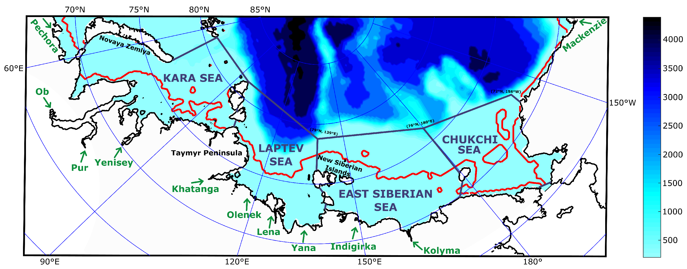
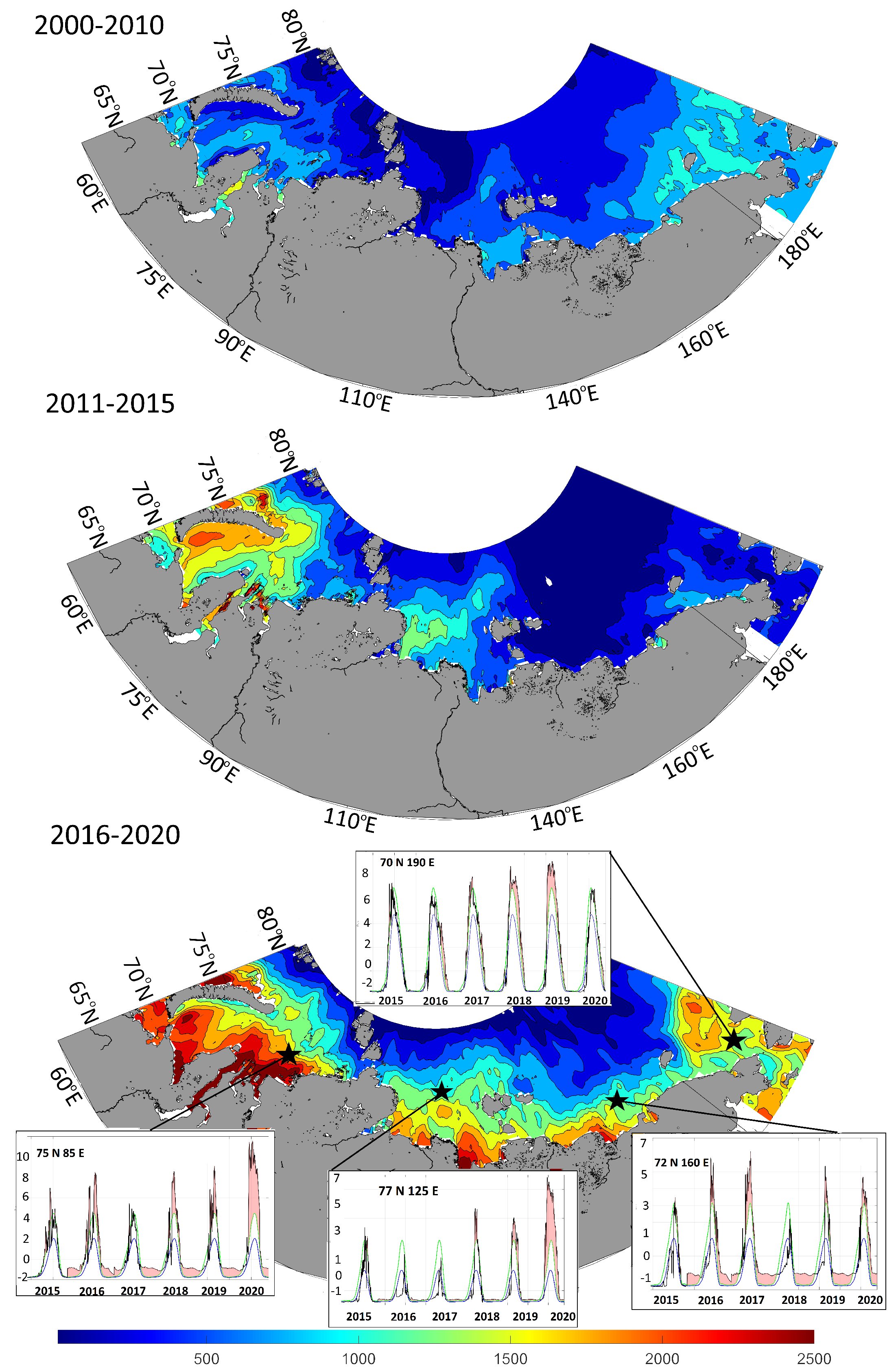
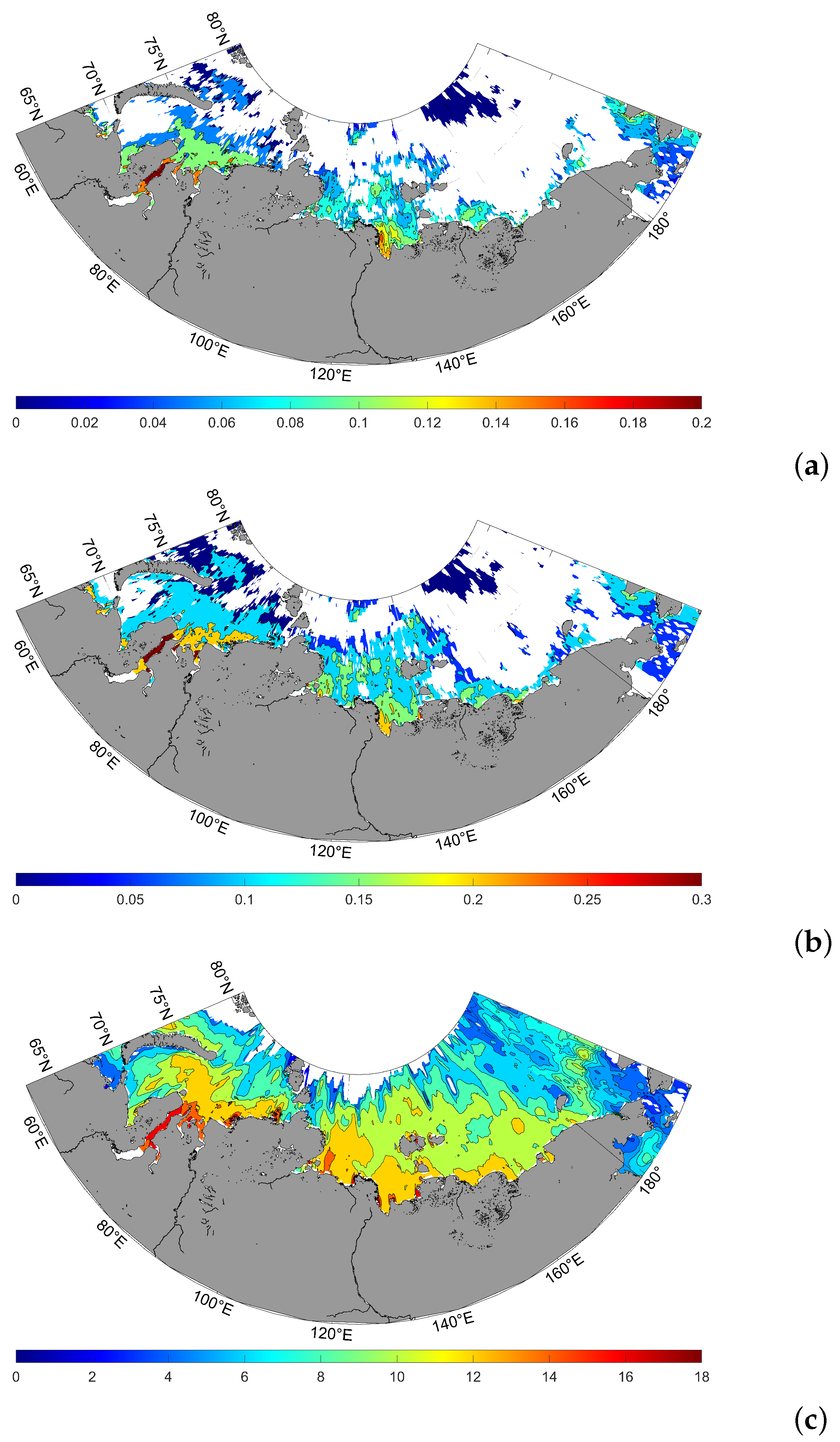
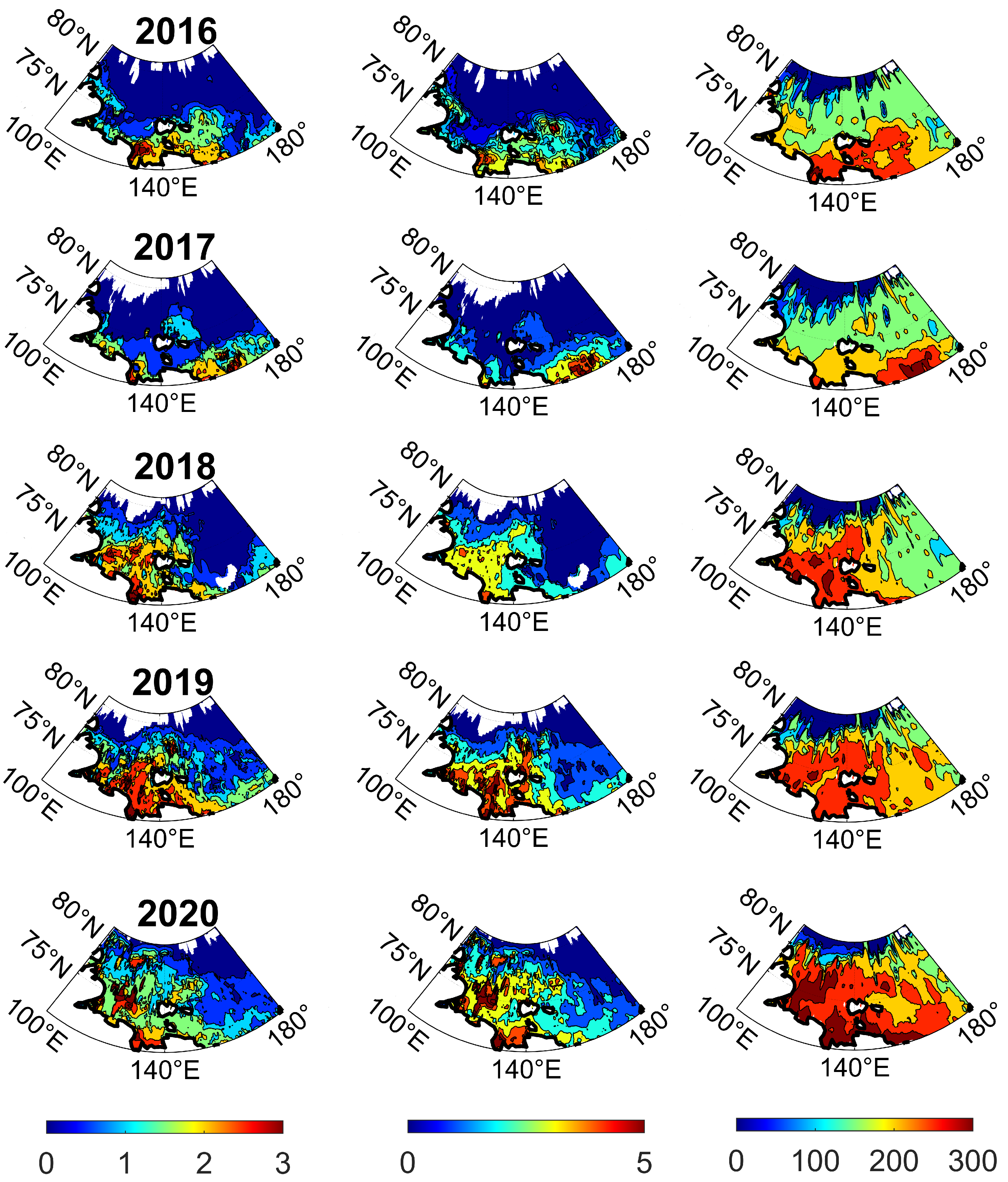
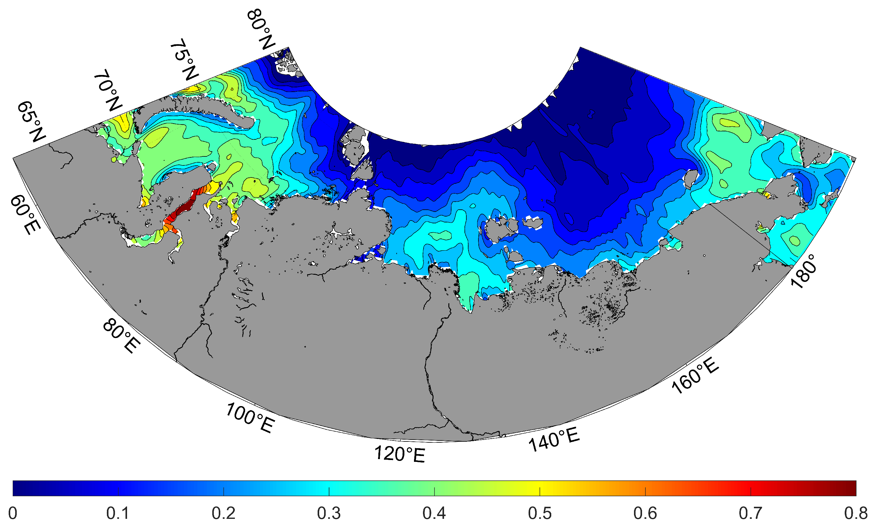
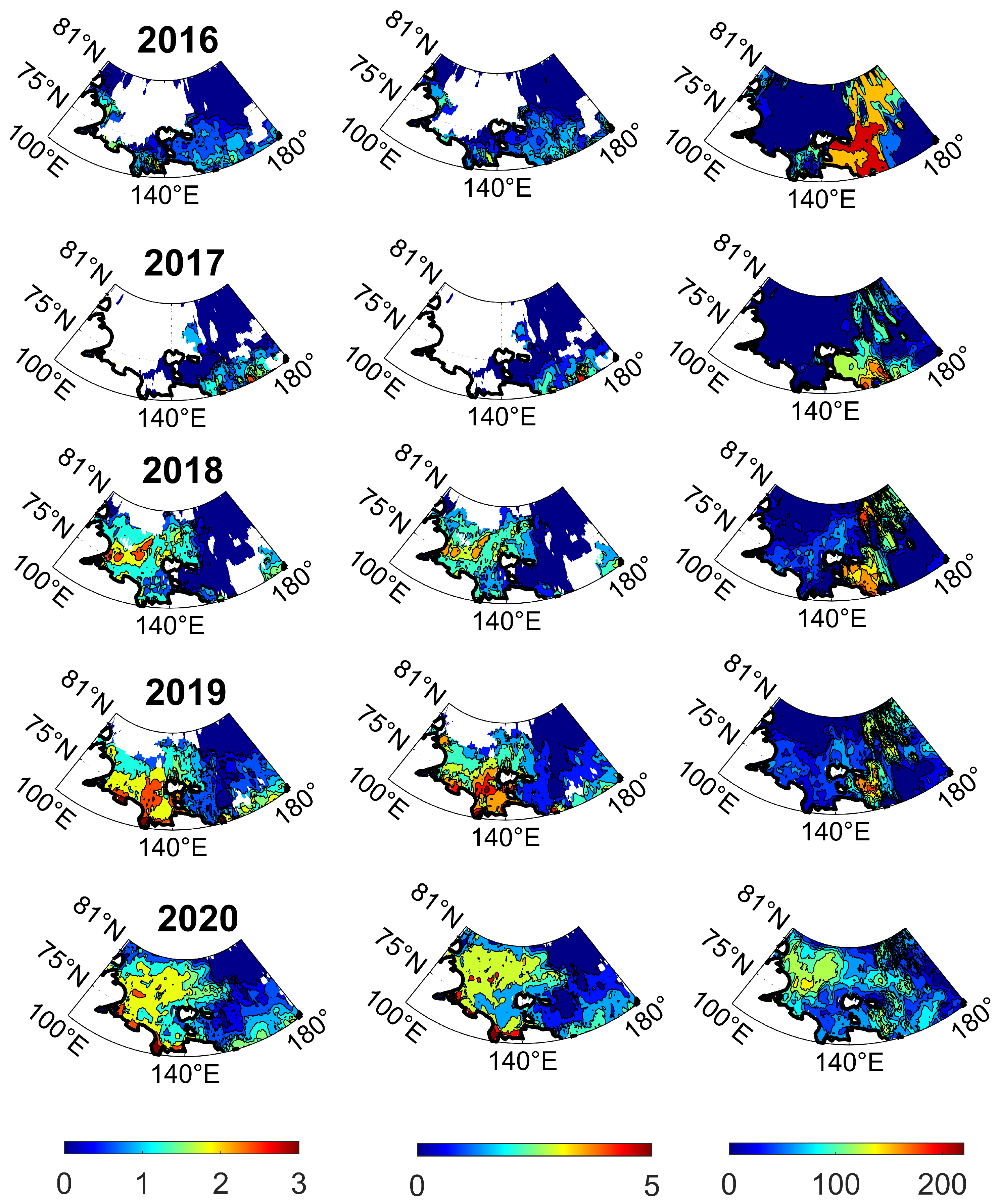
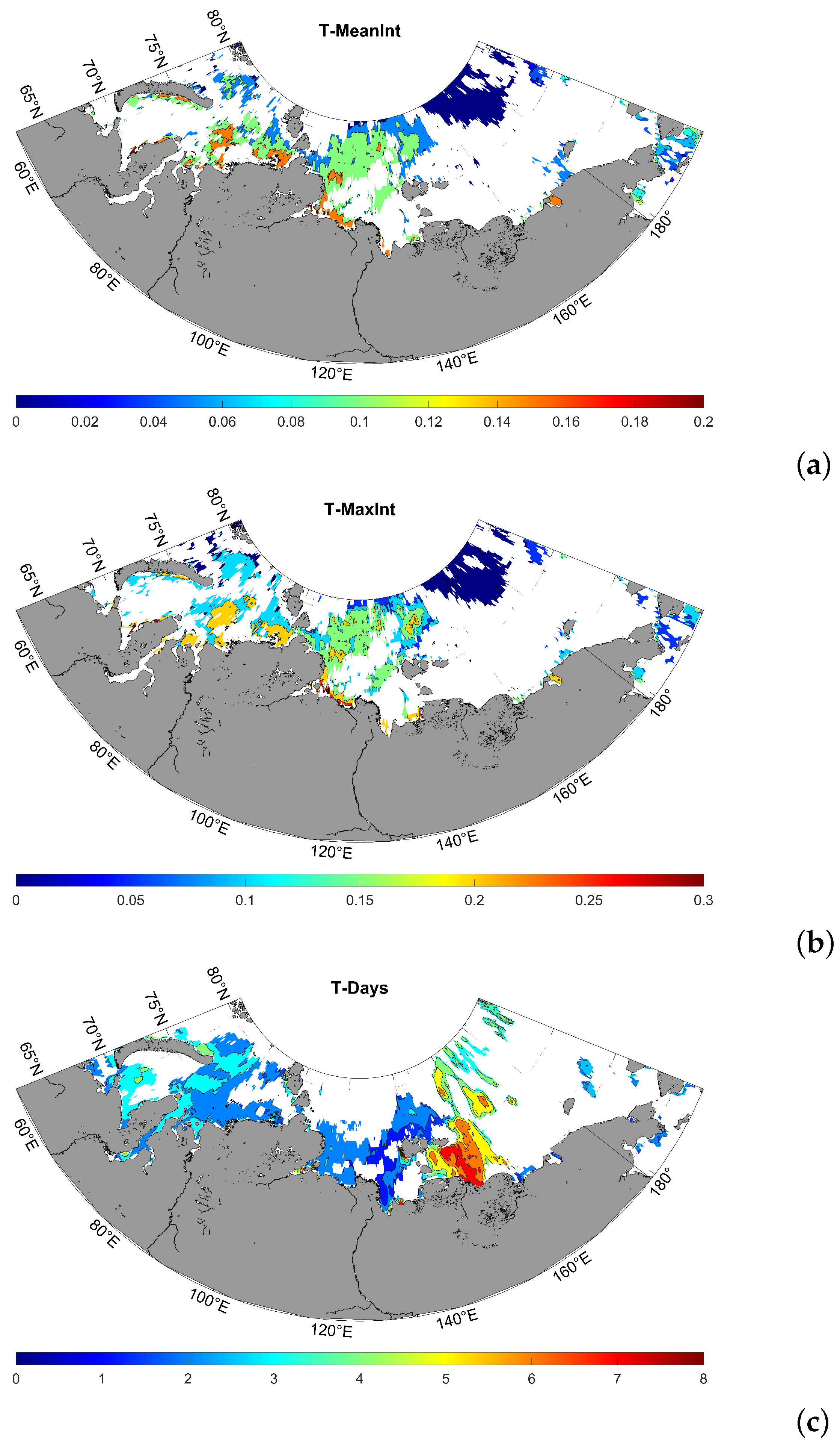
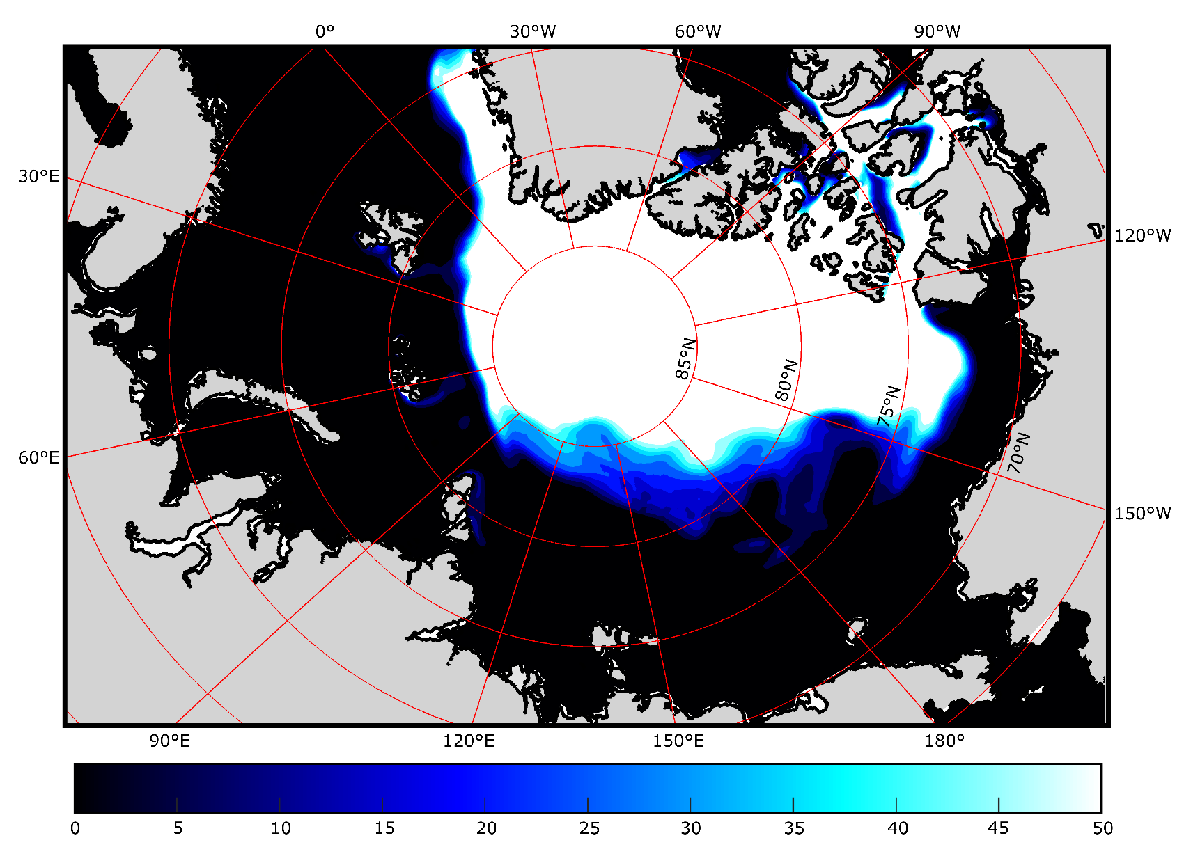
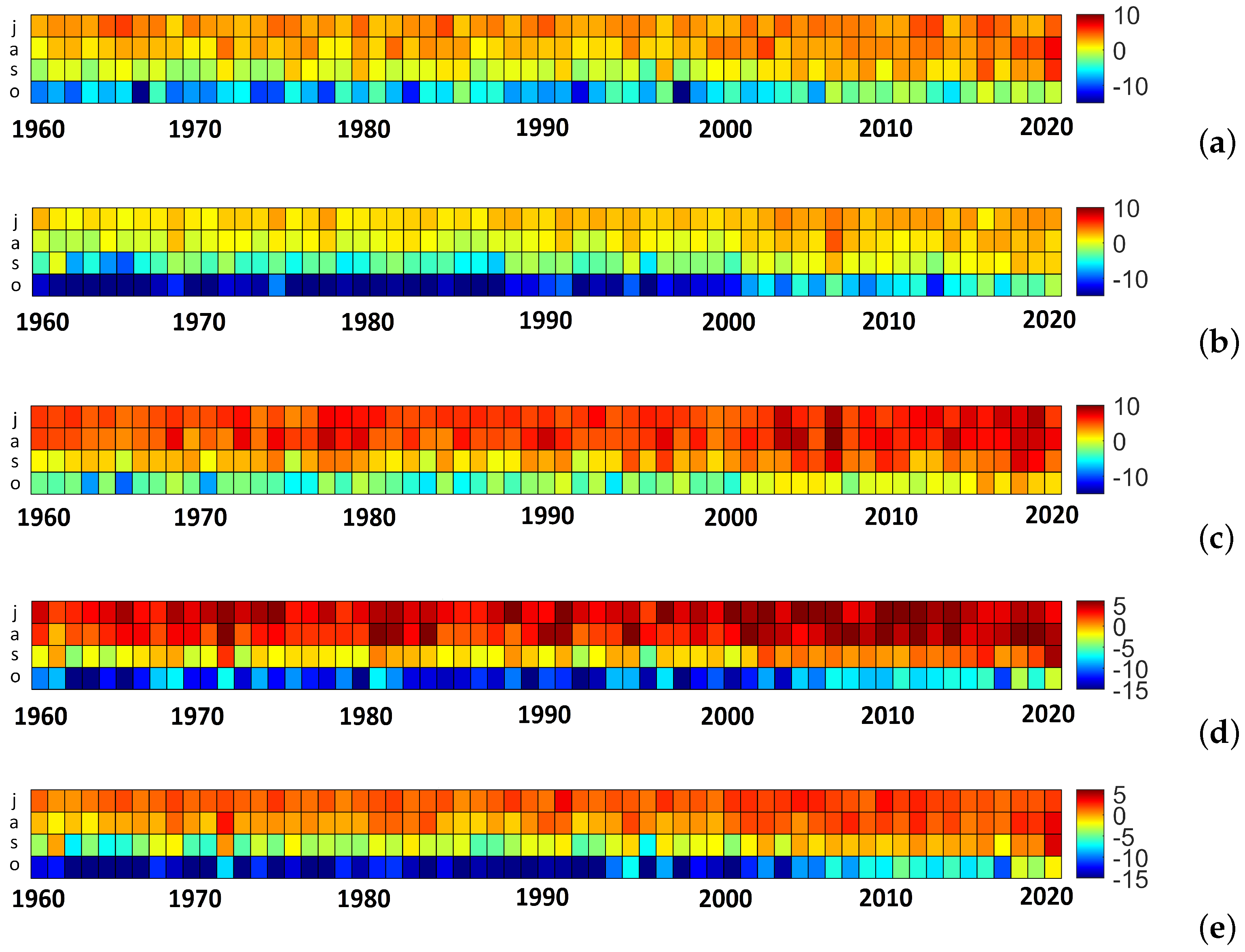
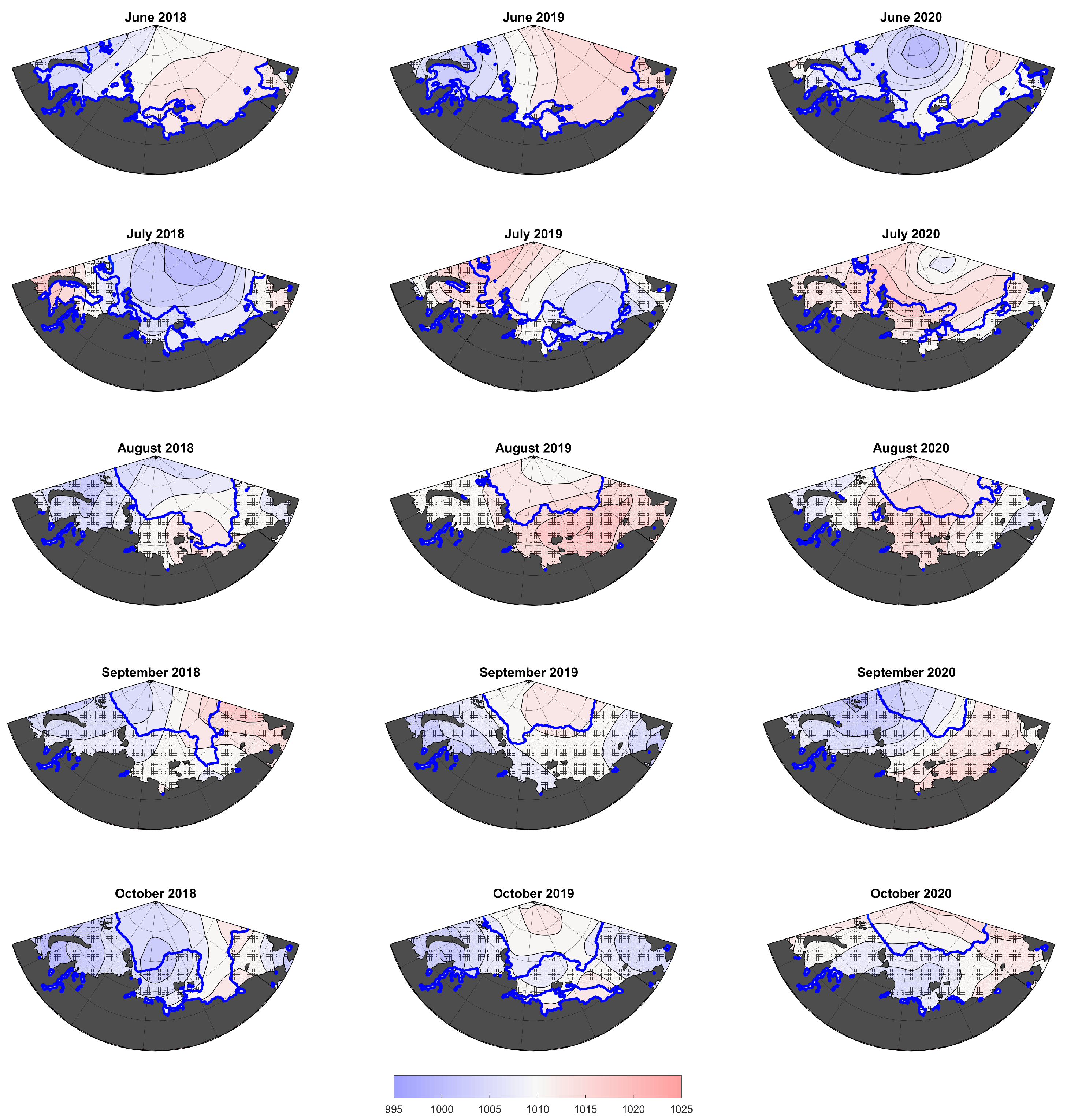
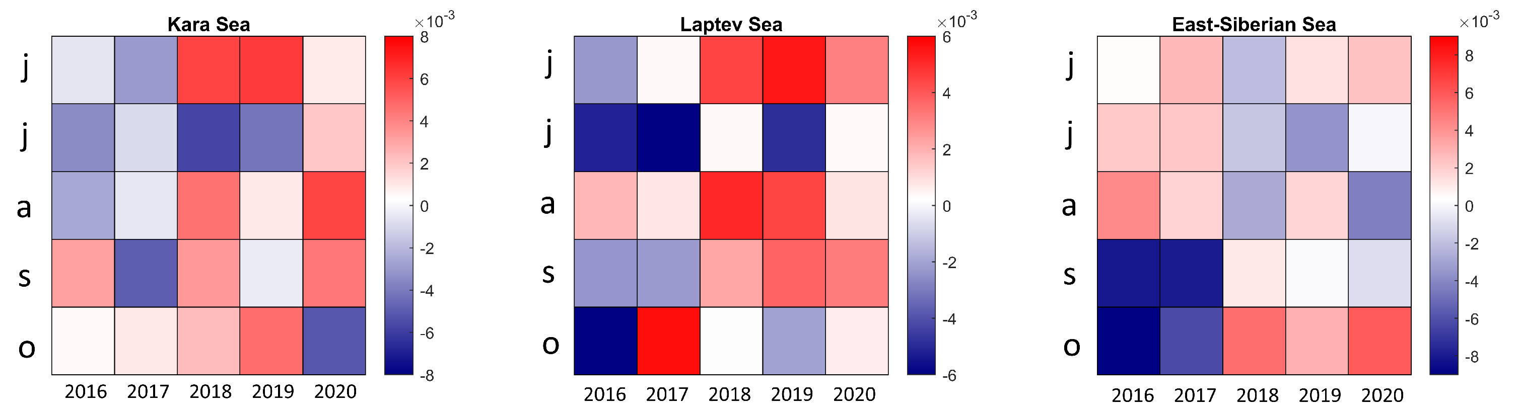
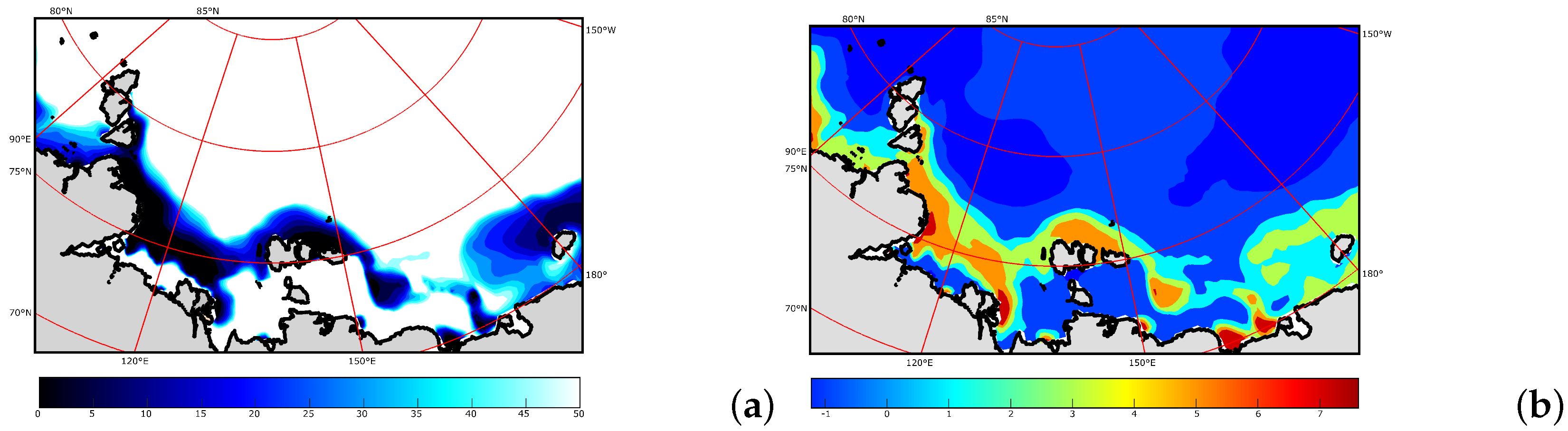
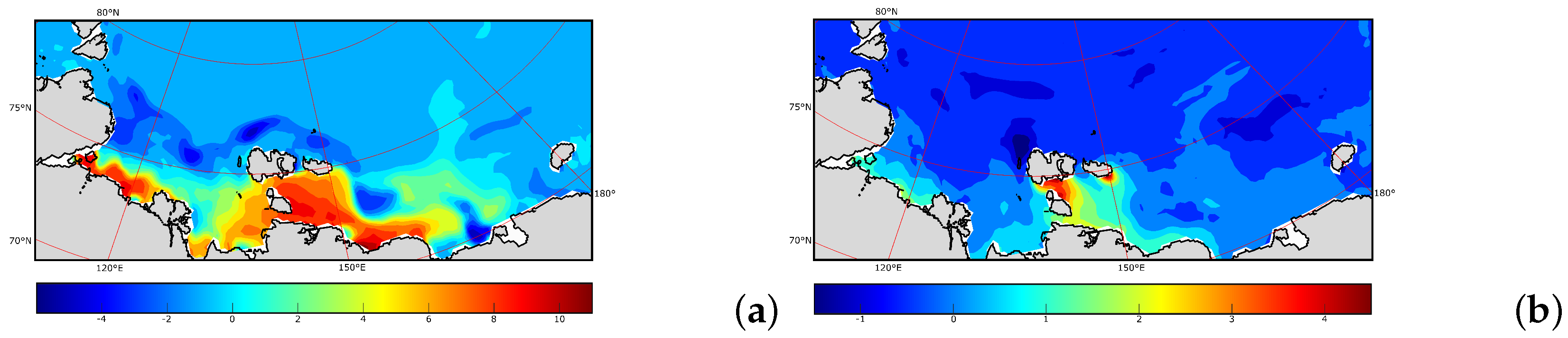
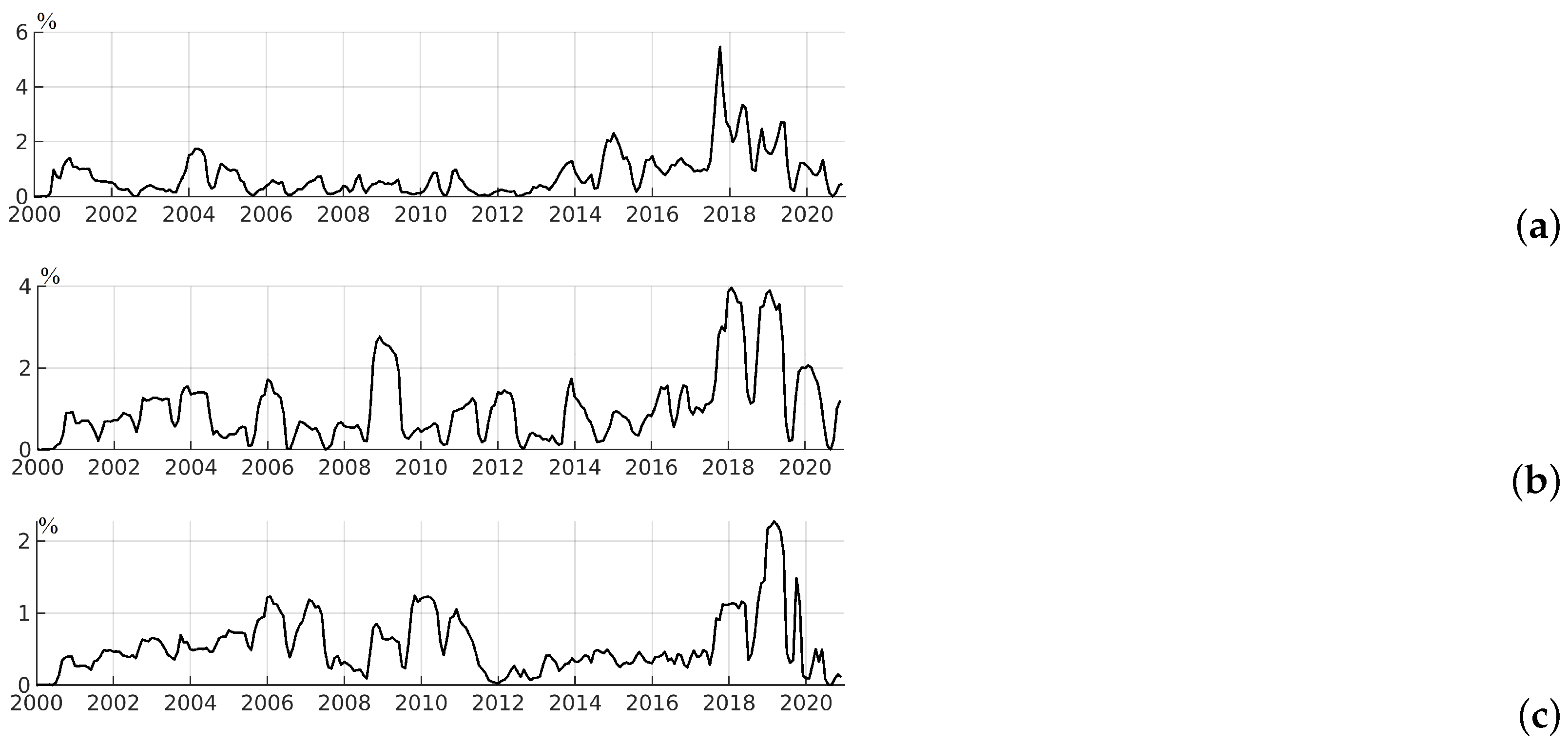
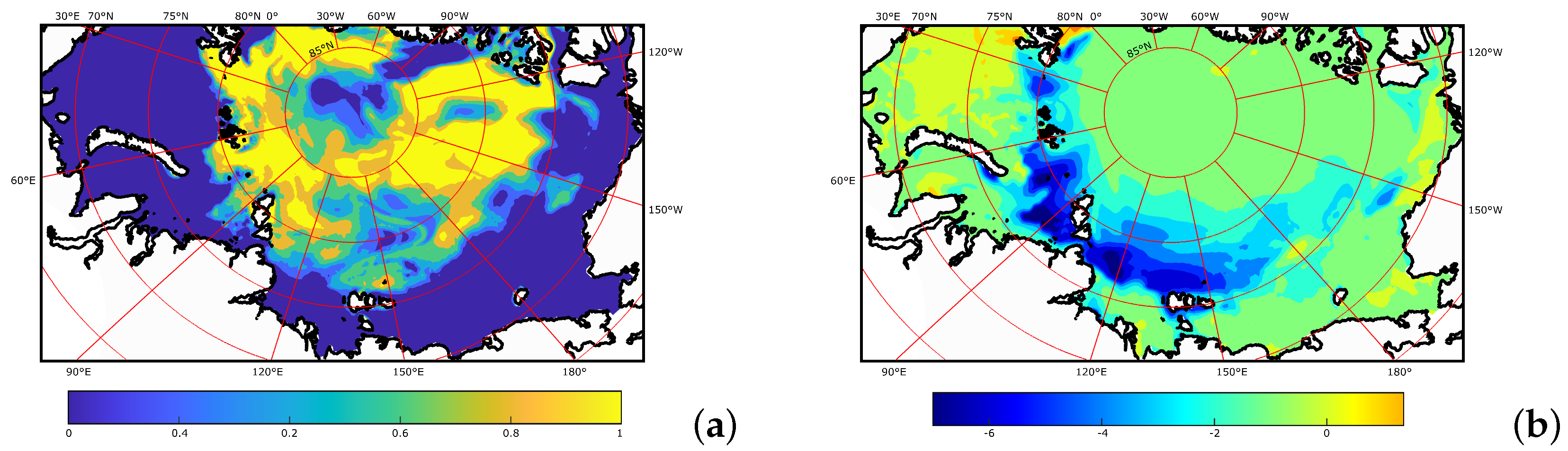
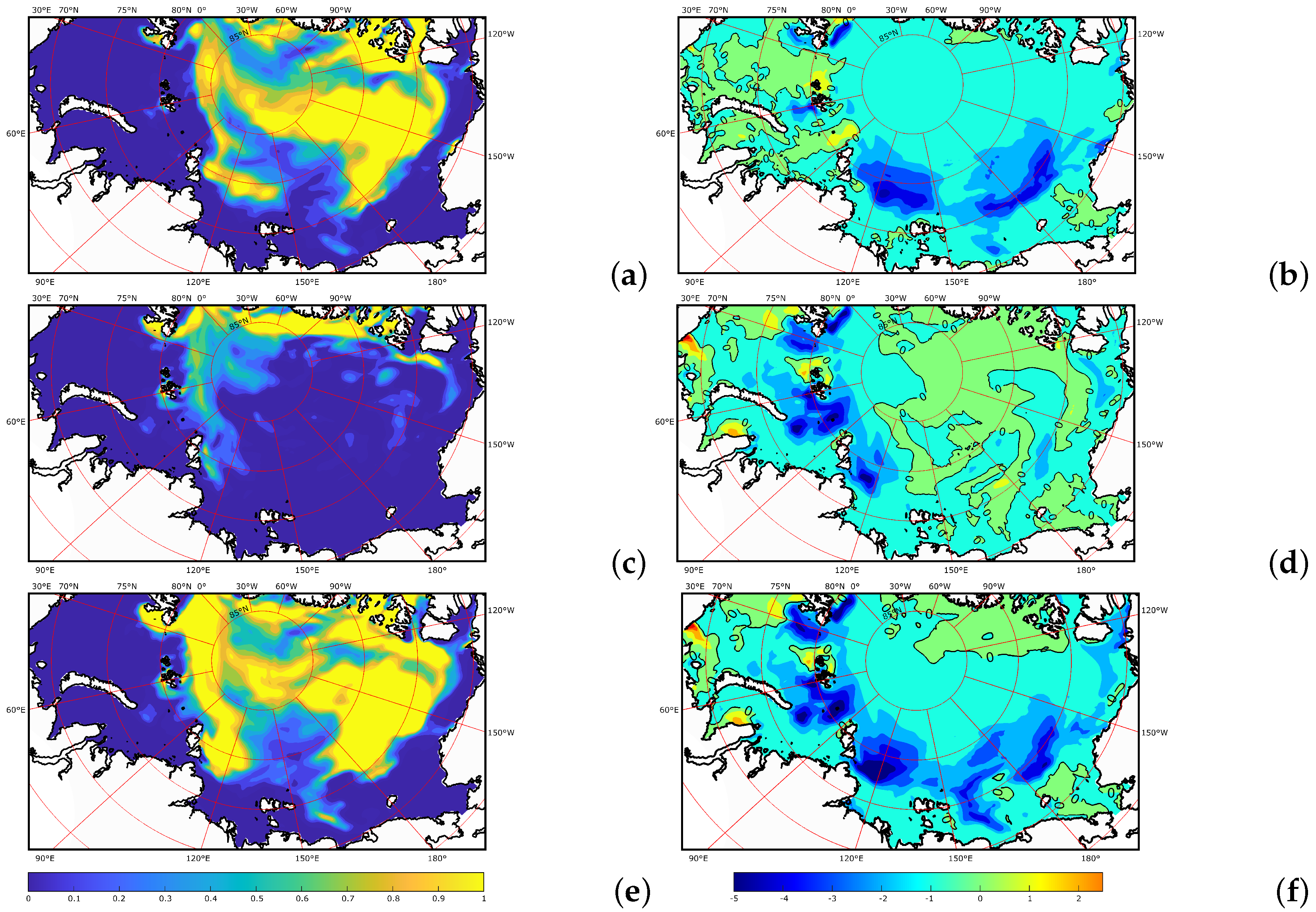
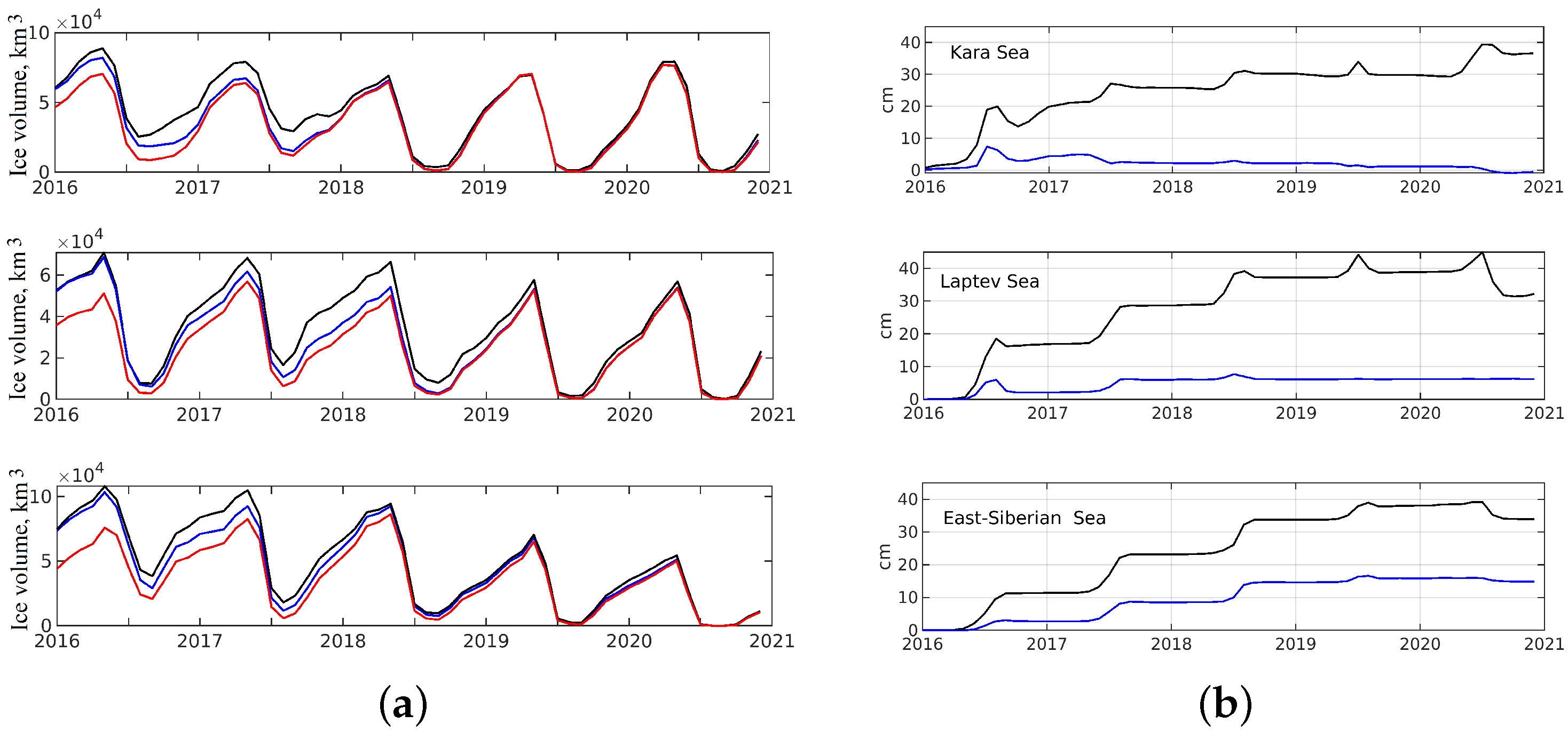
Table 1.
Annual mean surface air temperature anomalies averaged over latitude ranges of 60–70, 70–85, and 60–85N, relative to the average for the period 1961–1990 based on the results of the analysis of observations [23].
Table 1.
Annual mean surface air temperature anomalies averaged over latitude ranges of 60–70, 70–85, and 60–85N, relative to the average for the period 1961–1990 based on the results of the analysis of observations [23].
| 2007 | 2008 | 2009 | 2010 | 2011 | 2012 | 2013 | 2014 | 2015 | 2016 | 2017 | 2018 | 2019 | 2020 | |
|---|---|---|---|---|---|---|---|---|---|---|---|---|---|---|
| 60–70N | 1.5 | 1.3 | 0.4 | 1.0 | 1.6 | 1.5 | 1.0 | 1.7 | 1.9 | 2.7 | 1.8 | 2.1 | 2.4 | 2.9 |
| 70–85N | 2.4 | 2.1 | 2.6 | 1.9 | 3.1 | 2.9 | 1.9 | 2.6 | 2.5 | 3.9 | 2.7 | 3.0 | 3.4 | 3.6 |
| 60–85N | 1.5 | 1.6 | 2.3 | 2.2 | 1.4 | 2.2 | 2.2 | 3.3 | 2.2 | 2.5 | 2.8 | 3.2 |
Table 2.
Specifications of numerical experiments.
| Exps. | Peculiarity of | Period of | Initial Ice State | Initial Ocean |
|---|---|---|---|---|
| Experiment | Simulation | State | ||
| A0 | Control experiment | Jan 2000–Dec 2020 | Jan 2000 | Jan 2000 |
| A1 | No fast ice | Jan 2000–Dec 2020 | Jan 2000 | Jan 2000 |
| A2 | No riverine heat | Jan 2000–Dec 2020 | Jan 2000 | Jan 2000 |
| D1 | No ice drift | Jan 2020–Dec 2020 | Jan 2020 | Jan 2020 |
| Sensitivity to initial ocean and ice state | ||||
| 1 year | ||||
| B1 | Thick ice | Nov 2019–Dec 2020 | Nov 2003 | Nov 2019 |
| B2 | Cold ocean | Nov 2019–Dec 2020 | Nov 2019 | Nov 2003 |
| B3 | Thick ice, cold ocean | Nov 2019–Dec 2020 | Nov 2003 | Nov 2003 |
| 5 years | ||||
| B11 | Thick ice | Jan 2016–Dec 2020 | Jan 2004 | Jan 2016 |
| B33 | Thick ice, cold ocean | Jan 2016–Dec 2020 | Jan 2004 | Jan 2004 |
Publisher’s Note: MDPI stays neutral with regard to jurisdictional claims in published maps and institutional affiliations. |
© 2021 by the authors. Licensee MDPI, Basel, Switzerland. This article is an open access article distributed under the terms and conditions of the Creative Commons Attribution (CC BY) license (https://creativecommons.org/licenses/by/4.0/).
Share and Cite
MDPI and ACS Style
Golubeva, E.; Kraineva, M.; Platov, G.; Iakshina, D.; Tarkhanova, M. Marine Heatwaves in Siberian Arctic Seas and Adjacent Region. Remote Sens. 2021, 13, 4436. https://doi.org/10.3390/rs13214436
AMA Style
Golubeva E, Kraineva M, Platov G, Iakshina D, Tarkhanova M. Marine Heatwaves in Siberian Arctic Seas and Adjacent Region. Remote Sensing. 2021; 13(21):4436. https://doi.org/10.3390/rs13214436
Chicago/Turabian StyleGolubeva, Elena, Marina Kraineva, Gennady Platov, Dina Iakshina, and Marina Tarkhanova. 2021. "Marine Heatwaves in Siberian Arctic Seas and Adjacent Region" Remote Sensing 13, no. 21: 4436. https://doi.org/10.3390/rs13214436
Note that from the first issue of 2016, this journal uses article numbers instead of page numbers. See further details here.