High-Resolution Ocean Currents from Sea Surface Temperature Observations: The Catalan Sea (Western Mediterranean)

Abstract

Current observations of ocean currents are mainly based on altimetric measurements of Sea Surface Heights (SSH), however the characteristics of the present-day constellation of altimeters are only capable to retrieve surface currents at scales larger than 50–70 km. By contrast, infrared and visible radiometers reach spatial resolutions thirty times higher than altimeters under cloud-free conditions. During the last years, it has been shown how the Surface Quasi-Geostrophic (SQG) approximation is able to reconstruct surface currents from measured Sea Surface Temperature (SST), but it has not been yet used to retrieve velocities at scales shorter than those provided by altimeters. In this study, the velocity field of ocean structures with characteristic lengths between 10 and 20 km has been derived from infrared SST using the SQG approach and compared to the velocities derived from the trajectories of Lagrangian drifters. Results show that the SQG approach is able to reconstruct the direction of the velocity field with observed RMS errors between 8 and 15 degrees and linear correlations between 0.85 and 0.99. The reconstruction of the modulus of the velocity is more problematic due to two limitations of the SQG approach: the need to calibrate the level of energy and the ageostrophic contributions. If drifter trajectories are used to calibrate velocities and the analysis is restricted to small Rossby numbers, the RMS error in the range of 10 to 16 cm/s and linear correlations can be as high as 0.97.

1. Introduction

The observation of currents is of key importance for understanding the ocean and managing human activities at sea. However, observations are currently limited by sampling difficulties and the lack of satellite-based direct measurements. Indeed, the cost and difficulty of deploying in situ instruments, such as current meters or drifting buoys, lead to the need of using satellite measurements. At present, some direct satellite measurement do exist based on the Doppler signal of Synthetic Aperture Radars (SAR), but they are very limited, implying that currents have to be estimated by indirect approaches (see in [1], and references therein). To remediate such a limitation, the European Space Agency has recently started a pre-feasibility study of a new mission concept that would provide ocean surface current vectors at 1 km resolution for all the coastal ocean and shelf seas: the SeaStar concept [2]. Nevertheless, beyond the technological challenges such a mission may face, the limited availability of independent measurements of surface velocity vectors at an equivalent resolution is a major difficulty.

The most common approach to indirectly retrieve surface velocities relies on along-track measurements of Sea Surface Height (SSH) by altimeters, whose current sampling characteristics and noise level restricts its spatial resolution to scales larger than 50 km [1]. However, a better understanding of the dynamics in the upper layers of the ocean has shown that, under the appropriate conditions [3,4,5], their dynamics can be modeled using the Surface Quasi-Geostrophic (SQG) approximation [6]. This approach has been observed to be consistent with a wide range of ocean observations [7,8,9] and it has been successfully used to reconstruct velocities from Sea Surface Temperature (SST) measurements [10,11,12] and Sea Surface Salinity (SSS) [13]. The combination of the SQG framework with infrared measurements of SST has the potential to provide estimations of surface velocities comparable to those that will be provided by the SeaStar mission [14]. Nevertheless, its capability to reconstruct the velocity field at scales below altimeter capabilities has not been yet tested.

The Mediterranean sea is well suited for testing methods for deriving high-resolution velocities from infrared observations due to the large fraction of cloud-free images (∼40% in the Western Mediterranean, see Figure 1). Moreover, the Rossby radius in the Mediterranean is small (∼20 km) implying that the geostrophic approximation is valid at quite small scales. At the same time, the resolution attained by altimeters precludes to resolve a substantially fraction of the mesoscale dynamics in the Mediterranean, while SST observations may still remain adequate. The surface circulation in the Mediterranean is characterized by the entrance of fresh waters through the Gibraltar strait that then propagate anti-clockwise along the coast, particularly in the Western Mediterranean sea, e.g., [15]. The destabilization of these waters of Atlantic origin leads to the generation of vortices with sizes in the range of 50 to 100 km approximately, which have been studied with SSH and SST, e.g., [16,17,18,19].

Here, we explore the capability of the SQG framework to reconstruct the velocity field in its lower limits exploiting both the optimal conditions for using SST measurements in the Mediterranean and the validity of the geostrophic approach at scales significantly smaller than those captured by current altimeters. In particular, we focus on the reconstruction of the velocity field associated to coherent structures smaller than 20 km that were sampled by drifting buoys.

2. Theoretical Framework

Assuming that upper ocean velocities are non-divergent, a stream function can be defined such that the velocity $\overrightarrow{v}(x)$ is given by

$$\overrightarrow{v}(\overrightarrow{x},z)={\overrightarrow{e}}_z\times {\nabla }_z\psi (\overrightarrow{x},z),$$

where ${\overrightarrow{e}}_z$ is the vertical unit vector, $\overrightarrow{x}=(x,y)$, ${\nabla }_z=({\partial }_x,{\partial }_y,0)$, and $\psi (\overrightarrow{x},z)$ is the stream function. Invoking the principle of invertibility of Potential Vorticity (PV) [21], the stream function of a balanced flow can be diagnosed from the knowledge of PV in the ocean interior and buoyancy on the boundaries. In particular, the Quasi-Geostrophic (QG) PV anomaly $q(\overrightarrow{x},z)$ is given by

$${\nabla }_z^2\psi +\frac{\partial }{\partial z}\left(\frac{1}{n^2}\frac{\partial \psi }{\partial z}\right)=q,$$

(1)

with the hydrostatic equation providing the boundary conditions at the surface,

$$f_0{\left.\frac{\partial \psi }{\partial z}\right|}_{z=0}=b_s,$$

(2)

and at the bottom, at depth H,

$${\left.\frac{\partial \psi }{\partial z}\right|}_{z=-H}=0.$$

(3)

Here, $b(\overrightarrow{x},z)$ is the buoyancy, $b(\overrightarrow{x},0)\equiv b_s(\overrightarrow{x})$, and $n(z)$ is the Prandtl ratio, which is defined as the quotient between the Brunt–Väisälä frequency $N(z)$ and the Coriolis parameter $f_0$

$$n(z)\equiv \frac{N(z)}{f_0}.$$

(4)

Then, the stream function $\psi (\overrightarrow{x},z)$ can be recovered if the PV distribution $q(\overrightarrow{x},z)$ and the surface buoyancy $b_s(\overrightarrow{x})$ are known. In general, the PV is not known, unless in situ measurements are available, contrary to surface buoyancy, which can be estimated from satellite observations. Lapeyre and Klein [22] noted that, under the appropriate conditions, the PV is separable and in phase with surface buoyancy, implying that it can be written as

$$q(\overrightarrow{x},z)\approx \xi (z)b_s(\overrightarrow{x}),$$

(5)

which allows to solve the above differential equation, once the vertical variation of the Brunt–Väisälä frequency or the Prandtl ratio are known.

The solution to Equation (1) can be split into two contributions: a surface solution ${\psi }_{srf}(\overrightarrow{x},z)$ obtained taking $q(\overrightarrow{x},z)=0$ and $b_s(\overrightarrow{x})\ne 0$, and an interior solution ${\psi }_{int}(\overrightarrow{x},z)$ obtained taking $q(\overrightarrow{x},z)\ne 0$ and $b_s(\overrightarrow{x})=0$ [22]. For a constant stratification $n(z)=n_0$, the solutions to PV inversion problem with the PV given by Equation (5) are

$${\widehat{\psi }}_{srf}(\overrightarrow{k},z)=\frac{{\widehat{b}}_s(\overrightarrow{k})}{n_0{f}_{0}k}\frac{cosh\left[n_{0}k(H+z)\right]}{sinh(n_{0}kH)}$$

(6)

for the surface solution, see, e.g., in [23], and

$${\widehat{\psi }}_{int}(\overrightarrow{k},z)=-\frac{\xi (z){\widehat{b}}_s(\overrightarrow{k})}{f_0\left(k^2+\frac{1}{n_0^2{H}^2}\right)}.$$

(7)

for the interior one, see, e.g., in [24]. Here, the caret $\widehat{}$ stands for the 2D Fourier transform, $\overrightarrow{k}=(k_x,k_y)$ is the wavevector and $k=|\overrightarrow{k}|$ its modulus. Then, the total solution is given by

$$\widehat{\psi }(\overrightarrow{x},z)={\widehat{\psi }}_{srf}(\overrightarrow{x},z)+{\widehat{\psi }}_{int}(\overrightarrow{x},z).$$

Notice that the classical SQG solution [25]

$${\widehat{\psi }}_{srf}(\overrightarrow{k},z)=\frac{{\widehat{b}}_s(\overrightarrow{k})}{f_0{n}_{0}k}exp(n_{0}kz)$$

(8)

is recovered from Equation (6) in the limit $H\to -\infty$. Beyond the above, solutions for exponential stratification [26] and constant stratification with a mixed layer [27] are also available.

Lapeyre and Klein [22] and LaCasce and Mahadevan [28] proposed that the classical SQG solution Equation (8) can be used to derive the total stream function from buoyancy thanks to the non-orthogonality between the interior and surface solutions. In that case, the total solution would be

$$\widehat{\psi }(\overrightarrow{x},z)\approx c{\widehat{\psi }}_{srf}(\overrightarrow{x},z)=c\frac{{\widehat{b}}_s(\overrightarrow{k})}{f_0{n}_{0}k}exp(n_{0}kz),$$

(9)

where c is a constant to be fixed with independent observations. This theoretical framework can be applied to satellite observation of SST and/or SSS assuming that buoyancy at the surface is given as

$$b_s(\overrightarrow{x})\approx \alpha [T_s(\overrightarrow{x})-T_0]+\beta [S_s(\overrightarrow{x})-S_0],$$

(10)

where $T_s(\overrightarrow{x})$ and $S_s(\overrightarrow{x})$ are the corresponding sea surface observed values, $\alpha$ is the thermal expansion coefficient, and $\beta$ the haline contraction coefficent. If only SST are used, the constant c in Equation (9) not only accounts for the interior contribution [22], but also for the partial compensation between SST and SSS gradients [3,29]. The SQG approach can be generalized using the transfer function formalism, as proposed by Isern-Fontanet et al. [29] and González-Haro et al. [30] for surface currents. In that case, the surface stream function would be written as

$${\widehat{\psi }}_s(\overrightarrow{k})=F(k){\widehat{T}}_s(\overrightarrow{k}),$$

(11)

where $F(k)$ can be determined theoretically using Equations (6) and (7) or Equation (9) together with Equation (10) or, alternatively, estimated empirically using Sea Surface Height (SSH) and SST observations [29,30]. As a final remark, Isern-Fontanet et al. [3] proposed to use this framework to reconstruct the subsurface dynamics from high resolution SSH, which has been widely investigated during the recent years [27,31,32,33], and improved through the combination of SSH and SST measurements [34,35]. In those cases, high resolution SSH are needed, which will be available when the SWOT mission will be launched.

3. Materials and Methods

In this study, we focus on the reconstruction of surface velocities from high-resolution SST. Then, in order to explore the capability of the framework described in Section 2 to reconstruct the velocity field in its lower limits (<20 km), we have searched for small structures in the Mediterranean simultaneously sampled by surface drifters and infrared SST images. We selected those structures that could be tracked during a time period of at least 2 days and for which drifter trajectories and cloud-free satellite measurements were sampled with a maximum time difference of less than 12 h.

The database of drifting objects trajectories with vertical extensions of less than 1 m available at our institution was searched to identify looping patterns with diameters of the order of 20 km, or less (Figure 2). Then, those trajectories were compared to infrared SST satellite measurements. We found three coherent structures that could be followed during at least two to three days with SST images and simultaneously sampled with drifting buoys. This consisted of two coastal structures—a northwards propagating elliptical vortex with semi-axes of 5 and 10 km in front of Barcelona and a southwards propagating vortex or meander with a radius of 5 km in front of Valencia—as well as an open sea vortex with a radius between 5 and 10 km (Figure 2). The scarcity of available observations fulfilling the above requirements implied that we had to use not only standard devices such CODE drifters but also other drifting objects such as the dummies deployed during the exercises done by the Spanish Search and Rescue Service (SASEMAR). In particular, we used a dummy in horizontal position with a PK-2 buoy attached to the neck (see Figure 3). The PK-2 Satellite tracked Lagrangian drifting buoy has been developed at the ICM. It is composed of a low density polyethylene cylinder with 110 mm of diameter and 430 mm height. It hosts a high-performance GPS, with an error smaller than 6 m and a sampling frequency of 30 min [36]. The dummy in a horizontal position has almost no drag, which implies that it is very sensitive to wind, consequently, we focused on those situations with no wind. The CODE drifters were deployed during different experiments such as the CONECTA cruise [37].

The trajectories of the drifting objects were compared to the available sequence of thermal images and we found that the temporal evolution of these structures was very fast and barely captured by SST images. Two types of satellite data were used: Level 1 MODIS (Aqua and Terra) images downloaded from the NASA Goddard Space flight Centre (oceancolor.gsfc.nasa.gov (accessed on 9 September 2021)) and AVHRR images from NOAA-19 and MetOp platforms available at the ICM Coastal Ocean (coo.icm.csic.es (accessed on 9 September 2021)) in real time. MODIS data were processed using SeaDAS 7.0 to obtain SST and Brightness Temperature (BT), while AVHRR data already provided both SST and BT and no additional processing was applied. BT was preferred in front of SST due to its lower levels of noise [14]. In particular, we used the channel centered at 11 $\mathsf{\mu }$m for MODIS and the channel between 10.3 $\mathsf{\mu }$m and 11.3 $\mathsf{\mu }$m (channel 4) for AVHRR.

4. Framework Applicability

The applicability of the framework outlined in Section 2 depends on a combination of environmental [3,29] and dynamical [4,5] conditions. Among these conditions, there is the assumption that the flow is close to the geostrophic equilibrium. Moreover, as some of the ocean structures selected are located over the continental slope (see Figure 2), it is unclear whether that the classical SQG assumption may be suitable for retrieving ocean velocities ($H\sim$ 200 m).

The Rossby radius of deformation ${\ell }_R$ provides information about the scale above which the geostrophic approximation is valid. For a continuous stratification, it is given by ${\ell }_R=n_{0}H$, where H is a suitable vertical scale [38]. Taking it as the depth of the continental shelf ($H\sim 200$ m) and using stratification values of $n_0=50$ and $n_0=200$ typical of winter and summer respectively, we obtain Rossby radii of ${\ell }_R=10$ km and ${\ell }_R=40$ km. A more accurate determination of the Rossby radius requires to solve a Sturm–Liouville eigenvalue problem. According to Chelton et al. [39], the solution to this problem can be approximated as

$${\ell }_R\approx \frac{1}{\pi }{\int }_{-H}^{0}n(z)dz.$$

(12)

Its worth mentioning that this approximation is known to overestimate the Rossby radius providing radii systematically higher by about 6.5% [39]. The Brunt–Väisälä frequency $N(z)$ was estimated from the in situ temperature and practical salinity provided by the the World Ocean Atlas (2018) [40] using the TEOS-10 equation of state for sea water [41]. Then, Equation (12) was integrated at each available point (see Figure 4). Results show that the Rossby radius in this area is shorten than 10 km, which, a priory, implies that the geostrophic approximation can be used to derive the dynamics of the small structures selected for this study.

The next question is to define the transfer function that will be used to reconstruct velocities. The transfer function corresponding to the surface solution for a finite depth is given by Equation (6):

$$F_{srf}(k)=-\frac{g\alpha }{{\rho }_0}\frac{1}{n_0{f}_{0}ktanh(n_{0}kH)}$$

(13)

The limiting behavior of this transfer function is $F_{srf}(k)\sim k^{-2}$ for large scales (small k) and $F_{srf}(k)\sim k^{-1}$ for the small scales (large k). Using representative values of summer stratification and depth above the platform and in the blue sea, Figure 5 shows that the departure of the classical SQG behavior [25], i.e., the departure from $F_{srf}(k)\sim k^{-1}$, is important at scales larger than the scales here investigated pointing to the use of the classical SQG solution even on the continental platform.

The evaluation of the interior contribution given by the transfer function

$$F_{int}(k)=\frac{g\alpha }{{\rho }_0}\frac{\xi (z)}{f_0\left(k^2+\frac{1}{n_0^2{H}^2}\right)}$$

(14)

requires to evaluate the function $\xi (z)$. According to Lapeyre and Klein [22], it can be approximated as

$$f_0\frac{\partial {\overline{q}}_y}{\partial y}\approx \xi (z)\frac{\partial {\overline{b}}_y}{\partial y},$$

(15)

where ${\overline{q}}_y(y,z)$ and ${\overline{b}}_y(y,z)$ are the meridional averages of PV and buoyancy, respectively. In particular, the meridionally averaged PV is approximated by

$${\overline{q}}_y\approx f_0\frac{\partial }{\partial z}\left(\frac{{\overline{b}}_y}{N^2}\right),$$

(16)

taking advantage of the dominance of the stretching term. These quantities were also estimated using the World Ocean Atlas (2018) [40]. In particular, density $\rho (\overrightarrow{x},z)$ was computed from the in situ temperature and practical salinity using the TEOS-10 equation of state for sea water [41] and, then, used to estimate buoyancy

$$b(\overrightarrow{x},z)\equiv -g\frac{\rho (\overrightarrow{x},z)-{\rho }_0}{{\rho }_0}$$

(17)

using the mean density as the reference density ${\rho }_0$. PV was obtained from the buoyancy and the Brunt–Väisälä frequency using the approximation given by Equation (16). Once these quantities were computed, the meridional averages were obtained and the function $\xi (z)$ was estimated by least-squares fitting

$$\xi (z)=f_0\frac{\langle {\partial }_y{\overline{q}}_y{\partial }_y{\overline{b}}_y\rangle }{\langle {({\partial }_y{\overline{b}}_y)}^2\rangle }.$$

(18)

At the ocean surface, ${\xi }_s\equiv \xi (0)\sim 5\times {10}^{-6}{\mathrm{m}}^{-1}$ in the area under study (Figure 2) although certain seasonal variability can be observed. Using this value for $\xi$, the relative importance between the interior and the surface solution can be explored (Figure 5). On one side, it is also evident that the departures from the $F_{int}(k)\sim k^{-2}$ are observable at wavelengths longer than the ones of interest. On the other side, the relative importance of the interior solution to respect the surface solution has a seasonal dependence through its functional dependence on the stratification $n_0$. Despite the interior contribution at wavelengths longer than 5 km in summer, we applied the same transfer function during the whole year:

$$F_{srf}(k)\approx -\frac{g\alpha }{{\rho }_0}\frac{c}{n_0{f}_{0}k}.$$

(19)

5. Reconstruction of Velocities

Surface velocities were estimated from BTs using Equation (19). First, they were calibrated to the same dynamical range of the corresponding SSTs and gaps corresponding to clouds were filled using the same approach as in Isern-Fontanet et al. [3], while gaps due to land were set to zero. Surface buoyancy was calculated using the Equation of SeaWater TEOS-10 and, then, interpolated to a regular local mercator grid. Finally, a Fast Fourier Transform algorithm was applied to the interpolated surface buoyancy and Equation (9) was used to estimate the surface stream function with $z=0$ and $n_0=100$. The constant c was initially set to 1, although it was then modified when compared to surface drifters. Finally, the surface stream function in the real space was recovered applying the inverse Fourier transform with a high-pass Lanczos filter with a cut-off wavelength of ${\lambda }_{max}=70$ km.

The reconstruction of velocities from thermal measurements was performed applying a high-pass filter with a cut-off wavelength larger than the size the observed coherent structures. As a consequence, we assume that the contribution from the large-scale flow discarded by the high-pass filter can be approximated by a constant value vector ${\overrightarrow{v}}_{ls}=(u_{ls},v_{ls})$. Then, the reconstructed velocity $\overrightarrow{v}$ is given by

$${\overrightarrow{v}}_r=c{\overrightarrow{v}}_{sqg}+{\overrightarrow{v}}_{ls},$$

(20)

where ${\overrightarrow{v}}_{sqg}$ is the velocity derived using the SQG approach and c a constant value that takes into account the contribution of the interior PV at these scales as well as the partial compensation due salinity [3,29]. The calibration of both c and ${\overrightarrow{v}}_{ls}$ was obtained through least-squares fitting of the above model (Equation (20)) against velocities derived from drifter trajectories ${\overrightarrow{v}}_d$. The goodness-of-fit was then assessed using the Pearson correlation coefficient and the Root Mean Squared Error (RMSE) of velocities and a propagation direction, i.e.,

$${\epsilon }_v\equiv {\left[\sum \parallel {\overrightarrow{v}}_d-c{\overrightarrow{v}}_{sqg}-{\overrightarrow{v}}_{ls}{\parallel }^2\right]}^{\frac{1}{2}}.$$

(21)

The comparison between drifters was initially restricted to observations within a time period of ±24 h around the date of the SST image.

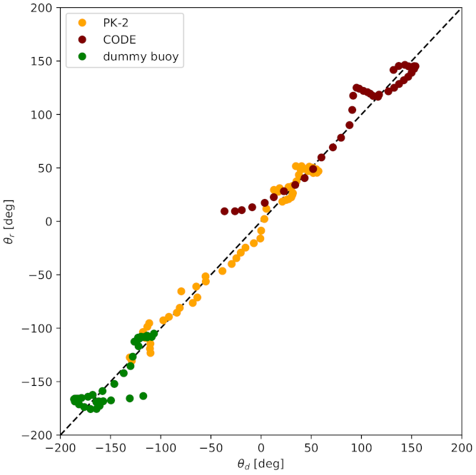
6. Comparison with Drifters

Figure 6 (upper left) shows the SQG velocity field for the coastal vortex propagating along the coast and the trajectory of the drifter, released about one day before the image capture and retrieved at 24 h later. It is clear that SQG velocities tend to be tangent to the drifter trajectory. SQG velocities were calibrated with Equation (20) using only drifter velocities with speeds $\parallel {\overrightarrow{v}}_d\parallel <50$ cm/s. This is motivated by the saturation in the velocity speed shown by the SQG velocities, which is evident in the scatter plot (Figure 6). This is typical from the ageostrophic corrections due to the increase of importance of the advective term for intense and curved trajectories. Indeed, the gradient flow approximation exhibits more intense velocities than its geostrophic flow counterpart. Fitting an ellipse to the drifter trajectory provides a major radius of 9.26 km and a minor radius of 4.53 km, suggesting Rossby numbers that can be close to 1, which implies significant ageostrophic contributions. Notice that correlations for the two components are bigger than 0.9 if only velocities such that $\parallel {\overrightarrow{v}}_d\parallel <50$ cm/s are considered (

Table 1. Comparison between SQG-derived velocities and velocities derived from drifter trajectories: start ($\Delta t_{-}$) and time ($\Delta t_{+}$) of the drifter data used in hours to respect the SST image date; maximum wavelength (${\lambda }_{max}$), correlations for zonal ($r_u$) and meridional ($r_v$) velocities, and correlation for velocity direction ($r_{\theta }$); and RMSE of velocity (${\epsilon }_v$) and direction (${\epsilon }_{\theta }$).

SST Image Date	$\mathbf{\Delta }{\mathit{t}}_{-}$	$\mathbf{\Delta }{\mathit{t}}_{+}$	${\mathit{\lambda }}_{\mathit{max}}$	${\mathit{r}}_{\mathit{u}}$	${\mathit{r}}_{\mathit{v}}$	${\mathit{r}}_{\mathit{\theta }}$	${\mathit{\epsilon }}_{\mathit{v}}$	${\mathit{\epsilon }}_{\mathit{\theta }}$	$({\mathit{u}}_0,{\mathit{v}}_0)$
	[h]	[h]	[km]				[cm/s]	[deg]	[cm/s]
2013-11-29 12:49	−23.9	−2.7	70	0.70	0.81	0.99	31	8.9	(7, −1)
				0.94 ${}^a$	0.97 ${}^a$	0.99 ${}^a$	9 ${}^a$	8.5 ${}^a$
2016-09-04 02:52	5.1	23.6	70	0.99	0.82	0.97	10	16.5	(17, 3)
2013-05-06 01:49	9.1	23.8	70	0.58	0.83	0.77	17	17.4	(−10, −3)
				0.66 ${}^b$	0.88 ${}^b$	0.85 ${}^b$	16 ${}^b$	15 ${}^b$	(−3, 0) ${}^b$

${}^a$ Same as above but restricting observations to those that $\parallel {\overrightarrow{v}}_d\parallel <$ 50 cm/s. ${}^b$ Same as above but displacing the trajectory to compensate time difference.

). This is also true for the velocity RMSE, which drops from 32 cm/s to 10 cm/s, if the most intense velocities are not considered.

Figure 6 (lower left) also shows the SQG velocity field associated to the second coastal coherent structure. The comparison between the SQG velocity field and drifter trajectories also shows a good agreement. However, its temporal evolution (Figure 7) shows that the coastal vortex moved by 0.05${}^{\circ }$ southwards during a time period of 36 h approximately while the time delay between the dummy’s deployment and the available SST was of 9 h. Assuming a constant propagation velocity, we estimate that the structure has propagated ∼1.4 km between this period of time (0.01245${}^{\circ }$). To face this problem, we moved the Lagrangian trajectory in the opposite direction of propagation of the meander taking into account its propagation velocity and the time between the images and the deployment of the dummy. If the drifter trajectory is displaced in the opposite direction to take this into account, we observe an increase on the correlations (Table 1). When comparing SST and drifter observations, we considered only the trajectory until 7 May 2013 at 2 am due to the increase of wind visible in the sudden change of direction of the dummy of Figure 2 and Figure 7.

The third example (Figure 8) corresponds to an open ocean situation outside the continental shelf. Its rapid evolution could be captured by four consecutive images. A CODE drifter was trapped in the core of the vortex during one day approximately and then escaped. We focused on its evolution after leaving the vortex core because there were no clouds hiding any part of the vortex. As in the previous examples, SQG velocities tend to be tangent to the trajectory of the drifters, and the scatter plot between the reconstructed velocities and the drifter velocities is reasonably good. Pearson’s correlation coefficient shows values between 0.80 and 0.97 (Table 1) and velocity RMSE of the order of 10 cm/s.

The comparison was extended to their directions defied as $\theta (\overrightarrow{x})\equiv arctan(\overrightarrow{v})$. It has the advantage that it is not affected by ageostropic corrections such as the centrifugal acceleration. Then, in addition to the Pearson correlation coefficient, the RMSE for the directions is given by

$${\epsilon }_{\theta }={\left[\sum {({\theta }_d-{\theta }_{sqg})}^2\right]}^{\frac{1}{2}},$$

(22)

Figure 9 shows the scatter plot between the angles of the reconstructed velocities and those from drifter trajectories for all the examples. Results show a striking correlation of 0.9. Notice that the two vortices in front of Barcelona have correlations above 0.95 and only the vortex/meander in the southernmost part of the domain has lower correlations, i.e., ∼0.8, (Table 1). As discussed above, Lagrangian measurements started 9 h later than the SST image was taken, which may affect the comparison for that case.

7. Summary and Conclusions

The validation of surface current vectors at 1 km provided by future missions such as the SeaStar mission concept will require developing and exploring complementary approaches to provided currents at similar spatial resolutions, at least in enough places and/or periods of time to carry on the validation. Here, we have investigated the potential of the the SQG approach applied in the north-western Mediterranean Sea to retrieve the velocity field of coherent structures with diameters less than 20 km from high resolution SST. Our results have confirmed that the Rossby radius is small enough to allow the use of the geostrophic approximation, although for small curvature radii the gradient flow approximation should be used. Our results have also confirmed that the SQG approximation can be used, even on the continental platform, to retrieve surface currents of coherent structures, provided that they have a strong signature in SST. These results open the door to use this area for validating future missions devoted to measuring high resolution velocity fields.

References

1. Isern-Fontanet, J.; Ballabrera-Poy, J.; Turiel, A.; García-Ladona, E. Remote sensing of ocean surface currents: A review of what is being observed and what is being assimilated. Nonlinear Process. Geophys. 2017, 24, 613–643. [Google Scholar] [CrossRef] [Green Version]
2. Gommenginger, C.; Chapron, B.; Hogg, A.; Buckingham, C.; Fox-Kemper, B.; Eriksson, L.; Soulat, F.; Ubelmann, C.; Ocampo-Torres, F.; Nardelli, B.B.; et al. SEASTAR: A Mission to Study Ocean Submesoscale Dynamics and Small-Scale Atmosphere-Ocean Processes in Coastal, Shelf and Polar Seas. Front. Mar. Sci. 2019, 6, 457. [Google Scholar] [CrossRef] [Green Version]
3. Isern-Fontanet, J.; Lapeyre, G.; Klein, P.; Chapron, B.; Hetcht, M. Three-dimensional reconstruction of oceanic mesoscale currents from surface information. J. Geophys. Res. 2008, C09005. [Google Scholar] [CrossRef] [Green Version]
4. Lapeyre, G. What mesoscale signal does the altimeter see? On the decomposition in baroclinic modes and the role of the surface boundary condition. J. Phys. Oceanogr. 2009, 39, 2857–2874. [Google Scholar] [CrossRef]
5. Ponte, A.; Klein, P. Reconstruction of the upper ocean 3D dynamics from high-resolution sea surface height. Ocean. Dyn. 2013, 63, 777–791. [Google Scholar] [CrossRef]
6. Lapeyre, G. Surface Quasi-Geostrophy. Fluids 2017, 2, 7. [Google Scholar] [CrossRef]
7. Le Traon, P.; Klein, P.; Hua, B.; Dibarbourne, G. Do altimeter wavenumber spectra agree with interior or surface quasi-geostrophic theory? J. Phys. Oceanogr. 2008, 38, 1137–1142. [Google Scholar] [CrossRef]
8. Lumpkin, R.; Elipot, S. Surface drifter pair spreading in the North Atlantic. J. Geophys. Res. Ocean. 2010, 115. [Google Scholar] [CrossRef] [Green Version]
9. Kim, S.Y.; Terrill, E.J.; Cornuelle, B.D.; Jones, B.; Washburn, L.; Moline, M.A.; Paduan, J.D.; Garfield, N.; Largier, J.L.; Crawford, G.; et al. Mapping the U.S. West Coast surface circulation: A multiyear analysis of high-frequency radar observations. J. Geophys. Res. 2011, 116, C03011. [Google Scholar] [CrossRef] [Green Version]
10. Isern-Fontanet, J.; Chapron, B.; Klein, P.; Lapeyre, G. Potential use of microwave SST for the estimation of surface ocean currents. Geophys. Res. Lett. 2006, 33, L24608. [Google Scholar] [CrossRef] [Green Version]
11. González-Haro, C.; Isern-Fontanet, J. Reconstruction of global surface currents from passive microwave radiometers. J. Geophys. Res. 2014, 119. [Google Scholar] [CrossRef]
12. Isern-Fontanet, J.; García-Ladona, E.; Madrid, J.; Olmedo, E.; García Sotillo, M.; Orfila, A.; Turiel, A. Real-time reconstruction of surface velocities from satellite observations in the Alboran sea. Remote Sens. 2020, 12, 724. [Google Scholar] [CrossRef] [Green Version]
13. Isern-Fontanet, J.; Olmedo, E.; Turiel, A.; Ballabrera-Poy, J.; García-Ladona, E. Retrieval of eddy dynamics from SMOS sea surface salinity measurements in the Algerian Basin (Mediterranean Sea). Geophys. Res. Lett. 2016, 43. [Google Scholar] [CrossRef] [Green Version]
14. Isern-Fontanet, J.; Hascoët, E. Diagnosis of high resolution upper ocean dynamics from noisy sea surface temperature. J. Geopys. Res. 2014, 118, 1–12. [Google Scholar] [CrossRef] [Green Version]
15. Poulain, P.; Menna, M.; Mauri, E. Surface Geostrophic Circulation of the Mediterranean Sea Derived from Drifter and Satellite Altimeter Data. J. Phys. Oceanogr. 2012, 42, 973–990. [Google Scholar] [CrossRef]
16. Puillat, I.; Taupier-Letage, I.; Millot, C. Algerian eddies lifetime can near 3 years. J. Mar. Syst. 2002, 31, 245–259. [Google Scholar] [CrossRef] [Green Version]
17. Rubio, A.; Arnau, P.; Espino, M.; Flexas, M.; Jordà, G.; Salat, J.; Puigdefàbregas, J.; Sánchez-Arcilla, A. A field study of the behaviour of an anticyclonic eddy on the Catalan continental shelf (NW Mediterranean). Prog. Oceanogr. 2005, 66, 142–156. [Google Scholar] [CrossRef]
18. Isern-Fontanet, J.; García-Ladona, E.; Font, J. The vortices of the Mediterranean sea: An altimetric perspective. J. Phys. Oceanogr. 2006, 36, 87–103. [Google Scholar] [CrossRef] [Green Version]
19. García-Olivares, A.; Isern-Fontanet, J.; García-Ladona, E. Dispersion of passive tracers and Finite-Scale Lyapunov Exponents in the Western Mediterranean sea. Deep-Sea Res. I 2007, 54, 253–268. [Google Scholar] [CrossRef]
20. González-Haro, C.; Ponte, A.; Autret, E. Quantifying Tidal Fluctuations in Remote Sensing Infrared SST Observations. Remote Sens. 2019, 11, 2313. [Google Scholar] [CrossRef] [Green Version]
21. Hoskins, B.; McIntyre, M.; Robertson, A. On the use and significance of isentropic potential vorticity maps. Q. J. R. Meteorol. Soc. 1985, 111, 877–946. [Google Scholar] [CrossRef]
22. Lapeyre, G.; Klein, P. Dynamics of the Upper Oceanic Layers in Terms of Surface Quasigeostrophy Theory. J. Phys. Oceanogr. 2006, 36, 165–176. [Google Scholar] [CrossRef]
23. Tulloch, R.; Smith, K. A New Theory for the Atmospheric Energy Spectrum: Depth-Limited Temperature Anomalies at the Tropopause. Proc. Natl. Acad. Sci. USA 2006, 103, 14690–14694. [Google Scholar] [CrossRef] [PubMed] [Green Version]
24. Klein, P.; Lapeyre, G.; Roullet, G.; Le Gentil, S.; Sasaki, H. Ocean turbulence at meso and submesoscales: Connection between surface and interior dynamics. Geophys. Astrophys. Fluid Dyn. 2011, 105, 421–437. [Google Scholar] [CrossRef]
25. Held, I.; Pierrehumbert, R.; Garner, S.; Swanson, K. Surface quasi-geostrophic dynamics. J. Fluid Mech. 1995, 282, 1–20. [Google Scholar] [CrossRef]
26. LaCasce, J. Surface Quasigeostrophic Solutions and Baroclinic Modes with Exponential Stratification. J. Phys. Oceanogr. 2012, 42, 569–580. [Google Scholar] [CrossRef] [Green Version]
27. Ponte, A.; Klein, P.; Capet, X.; Le Traon, P.; Chapron, B.; Lherminier, P. Diagnosing Surface Mixed Layer Dynamics from High-Resolution Satellite Observations: Numerical Insights. J. Phys. Oceanogr. 2013, 43, 1345–1355. [Google Scholar] [CrossRef]
28. LaCasce, J.; Mahadevan, A. Estimating subsurface horizontal and vertical velocities from sea surface temperature. J. Mar. Res. 2006, 64, 695–721. [Google Scholar] [CrossRef] [Green Version]
29. Isern-Fontanet, J.; Shinde, M.; González-Haro, C. On the transfer function between surface fields and the geostrophic stream function in the Mediterranean sea. J. Phys. Ocean 2014, 44, 1406–1423. [Google Scholar] [CrossRef]
30. González-Haro, C.; Isern-Fontanet, J.; Tandeo, P.; Garello, R. Ocean Surface Currents Reconstruction: Spectral Characterization of the Transfer Function Between SST and SSH. J. Geophys. Res. Ocean. 2020, 125, e2019JC015958. [Google Scholar] [CrossRef]
31. Klein, P.; Isern-Fontanet, J.; Lapeyre, G.; Roullet, G.; Danioux, E.; Chapron, B.; Le Gentil, S.; Sasaki, H. Diagnosis of vertical velocities in the upper ocean from high resolution sea surface height. Geophys. Res. Lett. 2009, 33, L24608. [Google Scholar] [CrossRef] [Green Version]
32. Qiu, B.; Chen, S.; Klein, P.; Ubelmann, C.; Fu, L.L.; Sasaki, H. Reconstructability of Three-Dimensional Upper-Ocean Circulation from SWOT Sea Surface Height Measurements. J. Phys. Oceanogr. 2016, 46, 947–963. [Google Scholar] [CrossRef]
33. Qiu, B.; Chen, S.; Klein, P.; Torres, H.; Wang, J.; Fu, L.L.; Menemenlis, D. Reconstructing Upper-Ocean Vertical Velocity Field from Sea Surface Height in the Presence of Unbalanced Motion. J. Phys. Oceanogr. 2019, 50, 55–79. [Google Scholar] [CrossRef]
34. Wang, J.; Flierl, G.; LaCasce, J.; McClean, J.; Mahadevan, A. Reconstructing the ocean’s interior from surface data. J. Phys Ocean. 2013, 43, 1611–1626. [Google Scholar] [CrossRef]
35. LaCasce, J.H.; Wang, J. Estimating Subsurface Velocities from Surface Fields with Idealized Stratification. J. Phys. Oceanogr. 2015, 45, 2424–2435. [Google Scholar] [CrossRef] [Green Version]
36. García-Ladona, E.; Salvador, J.; Fernandez, P.; Pelegri, J.; El’osegui, P.; Sńchez, O.; Madrid, J.J.; Pérez, F.; Ballabrera, J.; Isern-Fontanet, J.; et al. Thirty years of research and development of Lagrangian buoys at the Institute of Marine Sciences. Sci. Mar. 2016, 80, 141–158. [Google Scholar] [CrossRef] [Green Version]
37. Clavel-Henry, M.; North, E.W.; Solé, J.; Bahamon, N.; Carretón, M.; Company, J.B. Estimating the spawning locations of the deep-sea red and blue shrimp Aristeus antennatus (Crustacea: Decapoda) in the northwestern Mediterranean Sea with a backtracking larval transport model. Deep. Sea Res. Part Oceanogr. Res. Pap. 2021, 174, 103558. [Google Scholar] [CrossRef]
38. Cushman-Roisin, B.; Beckers, J. Introduction to Geophysical Fluid Dynamics, 2nd ed.; International Geophysics Series; Academic Press: Cambridge, MA, USA, 2011; Volume 101. [Google Scholar]
39. Chelton, D.B.; deSzoeke, R.A.; Schlax, M.G.; Naggar, K.E.; Siwertz, N. Geographical Variability of the First Baroclinic Rossby Radius of Deformation. J. Phys. Oceanogr. 1998, 28, 433–460. [Google Scholar] [CrossRef]
40. Boyer, T.P.; Garcia, H.E.; Locarnini, R.A.; Zweng, M.M.; Mishonov, A.V.; Reagan, J.R.; Weathers, K.A.; Baranova, O.K.; Seidov, D.; Smolyar, I.V. World Ocean Atlas 2018; Technical Report; NOAA National Centers for Environmental Information: Silver Spring, MD, USA, 2018. [Google Scholar]
41. Intergovernmental Oceanographic Commission; Scientific Committee on Oceanic Research; International Association for the Physical Sciences of the Oceans. The International Thermodynamic Equation of Seawater—2010: Calculation and Use of Thermodynamic Properties; Intergovernmental Oceanographic Commission, Manuals and Guides No. 56; UNESCO: Paris, France, 2010. [Google Scholar]
Figure 1. Probability of clear pixel for the time series (1982–2011) considered in the climatology of the maximum gradient of SST from University of Rhode Island (URI) Pathfinder 9 km frontal database (courtesy of Peter Cornillon Graduate School of Oceanography, University of Rhode Island (URI)). Figure taken from [20].
Remotesensing 13 03635 g001
Figure 2. (Top): Bathymetry of the southern part of the Catalan sea showing the trajectories of surface drifting buoys used in this study and the location of the area of study in the western Mediterranean Sea. (Bottom): Zoom of drifter trajectories with the drifter type and their size. The solid black line corresponds to the observed trajectory and the dot its initial position. From (left) to (right): Trajectory of a dummy buoy in front of the Valencia coast; trajectory of the CODE drifter released during the CONECTA cruise; and trajectory of the CODE drifter released in front of the Barcelona coast.
Remotesensing 13 03635 g002
Figure 3. Image of 2 June 2015 showing the dummy with the GPS transmitter (black and orange cylinder) attached to its neck used in the Valencia experiment. Copyright SASEMAR with permission.
Remotesensing 13 03635 g003
Figure 4. Rossby radius estimated from the World Ocean Atlas (2018) using the approximation provided by Chelton et al. [39] for January–March (left) and July–September (right). Solid black lines correspond to bathymetric lines drawn every 200 m.
Remotesensing 13 03635 g004
Figure 5. Surface transfer function F s r f ( k ) (left) and interior transfer function F i n t ( k ) (right), both at the ocean surface. The dashed black line corresponds to k 1 and k 2 , and the green band the range of scales of interest, i.e., between 1 and 20 km.
Remotesensing 13 03635 g005
Figure 6. (Left) BT of coastal coherent structures with the reconstructed velocity field. White line indicated the trajectory of the drifter used for the scatter plot of the second line and the metrics shown in Table 1. (Right) Scatter plot between velocities derived from drifters and those obtained from the BT images. White areas correspond mainly to land areas.
Remotesensing 13 03635 g006
Figure 7. Sequence of thermal images of the southwards propagation of the coastal perturbation in front of the Valencia coast. The solid black line corresponds to the observed trajectory. The dote indicates its initial position.
Remotesensing 13 03635 g007
Figure 8. (Left) BT of an open sea coherent structure with the SQG velocity field. While lines are the segments of drifters trajectories used in the metrics of Table 1 and the scatter plots at right. (Right) scatter plot between velocities derived from drifters and those obtained from the BT images. The white region delimitates approximately the coastal boundary..
Remotesensing 13 03635 g008
Figure 9. Scatter plot of the direction of the observed and reconstructed velocities for the three experiments.
Remotesensing 13 03635 g009