Article

Gradient Boosting Machine and Object-Based CNN for Land Cover Classification

1
Center for Applied Research in Remote Sensing and GIS (CARGIS), Faculty of Geography, VNU University of Science, Vietnam National University, Hanoi, 334 Nguyen Trai, Hanoi 11416, Vietnam
2
Geographic Information Systems Research Center, Feng Chia University, Taichung 40724, Taiwan
3
Faculty of Geography, VNU University of Science, 334 Nguyen Trai, Hanoi 11416, Vietnam
4
Department of Environmental & Geographical Science, University of Capetown, Rondebosh 7701, South Africa
5
School of Geographic Sciences, East China Normal University, Shanghai 200241, China
6
College of Geography and Environmental Sciences, Zhejiang Normal University, Jinhua 321004, China
*
Author to whom correspondence should be addressed.
Remote Sens. 2021, 13(14), 2709; https://doi.org/10.3390/rs13142709
Submission received: 19 June 2021 / Revised: 8 July 2021 / Accepted: 8 July 2021 / Published: 9 July 2021
(This article belongs to the Special Issue Applications of Remote Sensing for Resources Conservation)

Abstract

:
In regular convolutional neural networks (CNN), fully-connected layers act as classifiers to estimate the probabilities for each instance in classification tasks. The accuracy of CNNs can be improved by replacing fully connected layers with gradient boosting algorithms. In this regard, this study investigates three robust classifiers, namely XGBoost, LightGBM, and Catboost, in combination with a CNN for a land cover study in Hanoi, Vietnam. The experiments were implemented using SPOT7 imagery through (1) image segmentation and extraction of features, including spectral information and spatial metrics, (2) normalization of attribute values and generation of graphs, and (3) using graphs as the input dataset to the investigated models for classifying six land cover classes, namely House, Bare land, Vegetation, Water, Impervious Surface, and Shadow. The results show that CNN-based XGBoost (Overall accuracy = 0.8905), LightGBM (0.8956), and CatBoost (0.8956) outperform the other methods used for comparison. It can be seen that the combination of object-based image analysis and CNN-based gradient boosting algorithms significantly improves classification accuracies and can be considered as alternative methods for land cover analysis.

Graphical Abstract

1. Introduction

Machine learning methods have been developed to automate the analysis and enhance remote sensing observations by introducing new classifiers, segmentation, or optimization algorithms. These methods are efficient when applied to high spatial resolution data, including satellites, air-borne, and Unmanned Aerial Vehicle data. Among conventional methods, ensemble classifier random forest (RF), Neural network, and Support vector machine (SVM) techniques are regularly employed for image classification and other tasks (e.g., change detection) with considerable success. These methods have received much attention due to their ability to handle multi-dimensional data and perform well with limited training samples [1,2,3,4,5,6,7]. Typically, these conventional machine learning approaches have been applied using shallow classification techniques. However, the massive increase in the size of datasets (velocity, volume, variety) has resulted in a bottleneck in efficient data processing [8].
In more recent years, the advent of deep learning (DL) has led to renewed interest in neural networks. DL has demonstrated astounding capabilities, primarily attributed to the automated extraction of essential features, removing the need for identifying case-specific features. The driving force behind the success of DL in image analysis can be traced to the following three key factors: (1) More data available for training DNNs, especially in cases of supervised learning such as classification, where users typically provide annotations, for example in [9,10]; (2) More processing power, especially the explosion in the availability of Graphical Processing Units; (3) More algorithms [5,11,12,13]. Among different deep learning structures, the convolutional neural network (CNN) is a widely used method successfully applied to pattern recognition, natural language processing, landcover classification, and point cloud dataset processing. As they are more efficient for processing large datasets, the CNN is particularly relevant for tasks involving remotely sensed imagery and other spatial data. CNN has been used in a wide range of applications, particularly in the classification of high spatial resolution datasets [14,15,16], including LULC classification, scene classification, and object detection [15,16,17,18,19,20], and for annotation of point cloud datasets [21]. More recently, recurrent CNNs (R-CNNs) have been used in the analysis of very high spatial resolution datasets with considerable success. For example, R-CNNs have been used to overcome the scarcity of labeled training data to detect scalable old and new buildings [22], enable the regularization of the building footprint [23], and facilitate the rapid extraction of buildings through iterative inclusion of validated samples [24].
The structure of CNN in land cover classification depends on several factors, such as the number of convolutional layers, activation functions, loss functions [7,25,26], or shapes of input data, such as patch-based [27,28] or graph-based [29]. Moreover, the types of output, either scene-based [9] or pixel-based classes [12,30], influence the selection of classification methods. Some studies [13,31] have discussed how 1D and 2D graphs and line thickness improve the classification accuracy compared to several standard CCN-based methods, whereas others have attempted to integrate machine learning classifiers into CNN, as in [32]. The object-based image analysis (OBIA) has also been combined with CNN to take advantage of boundary delimitation of the former and spatial feature extraction of the latter method [33,34,35,36,37,38]. In these studies, a dense layer is used in the classification of image objects, although this classifier can be replaced with other algorithms and are potentially valuable in land cover analysis.
Another note on the uses of CNNs for remote sensing applications is on the importance of the band combinations for the improvement of classification accuracies. Numerous studies focused on the application of high-resolution images using the recently established state-of-the-art object-based CNN deep learning technique, where they utilized optimal band combinations (e.g., three-band combinations) and exhibited significant accuracies [39,40,41,42]. Furthermore, these works developed an automatic extraction framework for remote sensing applications from high spatial resolution optical images using CNN architecture in a large-scale application based on multispectral band combinations. These approaches offer potential choices of bands in multiple spectral satellite images but offer none for datasets with limited bands, such as RGB images in common UAVs or several high-resolution images (SPOT 7). In these cases, the spatial arrangement of objects is a significant contribution to the overall performance of land pattern classification.
Many recent studies have discussed the robustness of CNN and other ensemble algorithms in land cover analysis. In brief, CNN reveals its strength with unstructured data (images), while ensemble methods seem to be better suited to tabulated datasets. In general, gradient boosting [43,44,45] is an iterative learning process that learns from the errors made in the previous step for improved selection of weights in the subsequent iterations. This process develops a more complete picture of the dataset, and classification results are statistically reliable. A recent study that focused on land cover [46] compared CNN and gradient boosting for urban land classification and found small differences between those methods, although greater effectiveness of tree-based methods in land cover analysis for classification accuracy has been demonstrated [47]. The combination of CNN and gradient boosting algorithms may, indeed, improve the classification of satellite datasets. Nevertheless, complex human-made objects are replacing natural physical surfaces and, therefore, more efficient and effective models are increasingly needed. This study extends previous works [13,26,31,32] to test the potential use of gradient boosting algorithms as classifiers for the final layer of a CNN to improve the classification performance in terms of overall accuracy (OA) and error. The aim is to use SPOT7 imagery as input data, prepared in a sequence of image segmentation, feature extraction, and graph generation, followed by training of the proposed model for comparison with several other benchmarked methods. In summary, the main contributions of this manuscript include the construction of 2D input graphs from object features of the images extracted during image segmentation processes and the application of gradient boosting algorithms as a replacement for dense layers in CNN for more accurate land cover classification.

2. Data and Methods

2.1. Study Area and Training Data Preparation

Hanoi, the capital city of Vietnam, was selected as a case study because of its complex surface morphology and spatial mixture of various land cover types (Figure 1). The city boundary was extended in 2018 through a decision to merge neighboring provinces with different landscapes or historically distinctive morphological zones. The central-western part is a dynamic area because the residential areas are subject to ongoing development with a mix of high-rise buildings surrounded by open green spaces. The old French area is distinguishable by its house styles interspersed with small gardens, and it is also home to government buildings and affluent residential neighborhoods. On the other hand, the historical center remains unchanged, with its dense population concentration and small-facade houses. The automated classification of such areas can prove difficult because of the complex mixture of different land patterns, and accuracies are subject to the choice of the spatial and spectral resolution of input data.
In this study, SPOT 7 with 1.5 m spatial resolution in the panchromatic band and 6 m for multiple spectral ranges was used as the input dataset. For pre-processing, the process of combining multispectral and high-resolution panchromatic images with complementary characteristics often serves as an integral component of remote sensing mapping workflows [48,49]. Here, the fusion technique was applied to generate a higher resolution image with spectral information for multiple bands. Even though concerns have been raised about artifacts in fusion images, several studies have reported positive effects on the classification accuracy, although accuracy is subject to the detailed application of the fusion method. Fusion techniques are increasingly being used in remote sensing applications, such as Wavelength transformation, Browvey transformation, Intensity-Hue-Saturation fusion, Principal component transformation, and High pass filtering. In this study, the Gam Schmidt method [50] was used by simulating panchromatic bands and averaging multispectral bands. This method was found to be efficient in producing more natural colors. A more detailed specification of the dataset is presented in Table 1.
Segmentation was then carried out with the fusion images, using PCI Geomatics (evaluation version). This software uses the region-growing algorithm by selecting initial seed points and searching for similar neighbor pixels to form a larger region. The iteration is continued until desirable outputs are achieved by determining three parameters: scale, shape, and compactness (30, 0.75, and 0.5, respectively). The scale value influences how large the objects should be and is defined according to the spatial resolution of the input image. A sample area of the city covering all typical types of land patterns was chosen for verifying the proposed model. This subset of 54,234 segmented objects represents various land cover patterns, including six classes: house, impervious surface, water, bare land, vegetation, and shadow areas (Figure 1). All 54,234 objects in the study area were visually allocated into six classes, using higher resolution images as references and ground-truthing and ancillary documents, such as cultivation plans or current land-use/land-cover maps.
The inclusion of homogeneous pixels can result in valuable geometric shapes (i.e., square, round, and rectangle) that are useful for detecting specific human-made objects. With six input spectral bands, the algorithms produce 52 features, as shown in Table 2, including (i) spectral statistics of pixel values (min, max, mean, and standard deviations) and (ii) spatial metrics, such as Circularity, Compactness, Elongation, and Rectangular. These values can be used in tabulated form with traditional machine learning algorithms or hybrid models as reported in [11,12]. However, an alternative approach was proposed to generate plots from these values before feeding through the proposed model. Figure 1 shows the classes of the segmented objects that are set partly transparent for visualization and overlaid upon the natural-composite SPOT 7 image.

2.2. Gradient Boosting Classifiers

Gradient Boosting Machines (GBM) are powerful ensemble machine learning algorithms that employ decision trees to build up the classifiers. Technically, the algorithms apply iteration by adding models to correct weaknesses in prior models and improve overall performance accuracy. Among gradient boosting algorithms, XGBoost, LightGBM, and CatBoost are often considered as successful classifiers for various applications [44,45,51]. XGBoost uses the pre-sorted and histogram-based algorithm for estimating best splits and employs parallel processing with a handling capacity of missing values and minimization of over-fitting. In addition, this algorithm is based on a leaf-wise pruning strategy that leverages deep searches for an optimal solution, and the gradient descent algorithm minimizes errors.
LightGBM, proposed by Microsoft, is a recently developed gradient boosting algorithm or tree-based learning algorithm. It was developed to improve predictive efficiency, handle large datasets, and reduce training time, and is typically recommended for tabular datasets. LightGBM differs from other tree-based methods by implementing leaf-wise splits (Figure 2), which create more complex trees that are more efficient in reducing loss and resulting in higher accuracy. The split is based on a novel sampling method named Gradient-Based One Side Sampling [52], in which data with small gradients are excluded, and the rest is used for estimation of information gain and tree growth. This algorithm is controlled by a group of several parameters, including (1) boosting parameters, such as Max_depth, Learning_rate, Max_leaf_node, and gamma, and (2) learning task parameters, such as loss function type, evaluation metric, and number of iterations. These parameters control how leaves grow, as briefly shown in (Figure 2). As the tree grows, the model becomes more complex, the loss is reduced, and the algorithm learns faster. One of the limitations of such an algorithm is that over-fitting may occur if the dataset is small and a proper set of model parameters is required to avoid it.
Catboost, developed by Yandex, is a challenger to the previous two algorithms and is currently receiving close attention from data science communities. It has proved to be more effective than others without pre-processing requirements, and handling of over-fitting is avoided by the ordered boosting approach used in Catboost. During training, consecutive symmetric decision trees are built with reduced loss in comparison to others. The symmetrical trees are not a feature of other gradient boosting methods, and faster training is also achieved.

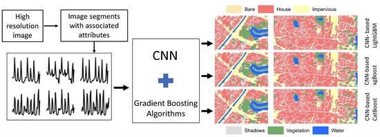
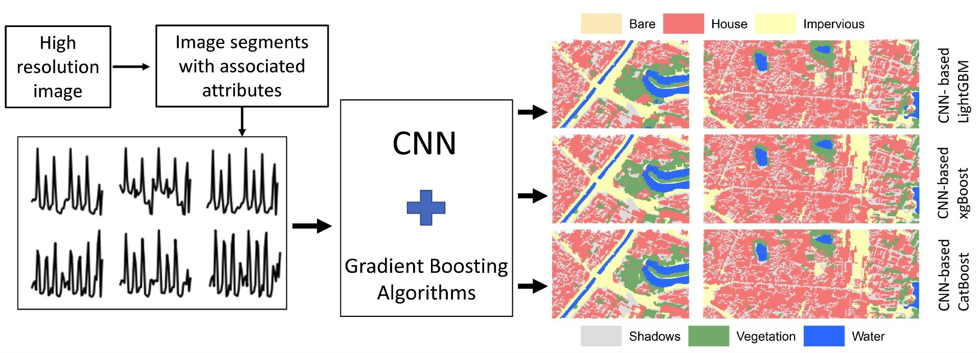
2.3. Object-Based CNN with GBM Algorithms

The proposed CNN structure is based on several successful models in land cover classification, such as the number of hidden layers, feature maps, and activated and loss functions [13,31]. The proposed hybrid model is illustrated in Figure 3 with several sequential steps. Step 1: A high-resolution image is segmented with various parameters, namely scale, compactness, and shape. These parameters should be tuned through a trial-error process to generate the most optimal boundary of potentially similar pixels. After segmentation, spectral and spatial metric features (Table 2) are associated with each object. Step 2: Because features are measured in different units and scales, a normalization step is required to ensure all features have a similar scale. A simple method (x–min)/(max-min) is applied to keep the original data distribution. Then, the normalized data are plotted in two-dimensional space. The plots are used as input patches that are fed into the CNN during the training stages. The total number of all image objects is randomly split into training/validation datasets and test sets. This hold-out method is commonly used in the CNN-based method rather than cross-validation because of the large amount of training data, representing the entire study area well. Step 3: the model is trained with the categorical log-loss function with fully connected layers as the classifiers. Step 4: Training data are fed again into the trained model from the previous step. However, the last dense layer is extracted to build up another training dataset, which is then used to learn three gradient boosting algorithms.
A more detailed structure of the CNN is presented in Figure 4. It consists of a sequence of layer stacks, in which the two first convolutional layers map similar grids over input images and sequentially map smaller grids. The leaky ReLU activation function is used during the training course to transform the feature spaces. Dropout is also applied to avoid over-fitting, in which neurons are turned off basing on their assigned probabilities during the forward stage. The output is flatted before feeding to the fully connected layer (FCN). This layer acts as a hidden layer in neural networks and outputs the probability for each class. After training the model with FCN, the last layer is replaced using gradient boosting algorithms to improve the prediction accuracy.

2.4. Accuracy Assessment

For multiple classification tasks, several statistical indicators are used for validating classifiers’ performances. Multiple errors and overall accuracy are used to validate the model, and the categorial_logloss functions are used for training. This loss function is the default option (such as Sparse Multiclass Cross-Entropy Loss and Kullback–Leibler Divergence Loss, among others) and is preferred for multiclass classification problems and can be explained as follows:
L X i Y i =     j = 1 c y i j log p i j
where Y i y i 1 , y i 2 ,   y i 6 is a one-hot encoded target vector representing six land cover classes. The y i j = 1 if i th element is in the class j; otherwise, y i j = 0 . p i j = f X i   = Prob shows that i th element is in class j . This function estimates the average difference between predicted and observed classes, and a score is calculated. Moreover, the study also compares the CNN-based gradient boosting algorithms’ performance with traditional classifiers, such as Random Forest and Support Vector Machine; therefore, the Root Mean Square Error (RMSE) and Overall Accuracy (OA) are also used. In addition, the model was interpreted using the salient map method that estimates the prediction capabilities (gradient of loss functions) for specific classes of each input feature.

3. Result and Discussions

The input images take the form of a graph representing the object’s features, as presented in Table 2. The input data were normalized to a similar value range [0–1] before being plotted and saved to single-band images. During the training dataset preparation, the plot lines’ weight impacts the edges’ recognition in the plots, as discussed in the study [13]. In this regard, we defined the line weight = 2, image size = 76 × 76, line color = black, and background = white, to generate 54,234 plots/figures in total. An illustration of the conversion from tabulated data to plots is shown in Figure 5. Among the figures, 50,234 were used for training, and 4000 plots were kept out of the training stage for visualization. The proportion of classes in the training data are bare soil = 890 images, impervious = 4716, shadows = 7786, vegetation = 6502, water = 330, and house = 30.010 (Table 3). It could be seen that the training dataset is unbalanced between a number of training data points among classes because of the dominance of houses in the urban area.
The applications of CNNs typically use trained networks and retrain them with new land cover datasets [30]. However, this study did not follow this strategy because the training data have different perceptions, which represent feature variation in one gray band image format. The training process would learn edge differences, which are generated considering changes in image objects’ spectral and spatial information (Figure 5). In this regard, the proposed model is trained from scratch with a proportion of samples, as shown in Table 3.
In the training stage, the training dataset (50,234 figures) was randomly split into training data (80%, 40,188 figures) and test data (20%, 10,046 figures). Because this study consists of multiple classification tasks, and the categorial_logloss function is used, the object labels were encoded with the one-hot method. In this regard, an array, for example, [0,0,0,0,0,1], represents a water object and similar arrays represent other classes depending on the location of the “1” value. Moreover, the ADAM optimizer was used with learning rate = 0.00025 and batch size = 512. More input images are generated through data augmentation/rotation during the training stage, and they are shuffled before each epoch. The model was trained in 300 epochs in TensorFlow on an 8-cores CPU and an NVIDIA GTX 1070 GPU.
Before gradient boosting algorithms are replaced for the classification task, the CNN with fully connected layers was trained, and the categorical log-loss was used as the objective function. The variation of log-loss is presented in Figure 6, in which, after the 120th epoch, the log-loss value seems to vary in a smaller range. At the 300th epoch, the log-loss fluctuation is so slight that we could consider terminating the training process and use the trained model for the next step.
The training data are again fed to the trained model, but the dense layer (before being fully connected) is extracted to form a new training set (40,188 instances, 128 features) and test set (10,046 instances, 128 features), respectively. These data were used to learn the gradient boosting algorithms, and the results are shown in Table 4. On the left side are values extracted from CNN with a fully connected layer and CNN’s with SVM, XGBoost, LightGBM, and CatBoost to replace the fully connected layer. These models were trained with plotted images, as explained in the previous section. Moreover, we considered verifying these algorithms with a dataset with the original 52 features, as illustrated in Figure 5. The results are shown on the right side of Table 3. It could be seen that CNN-CatBoost (OA = 0.8956) and CNN-LightGBM (OA = 0.8956) achieve the highest overall accuracies and the smallest errors. Thus, the CNN-based classifiers show improvements compared to traditional methods, which were run with the tabulated dataset. Furthermore, the higher features of the CNN-based gradient boosting (128) might result in higher accuracy of these models over the tabulated dataset (52 features).
For a more detailed analysis of the CNN-based methods, the confusion matrix is also shown in Table 4 and Table 5. For example, in looking at the Producer Accuracy, there is a high probability of misclassification between Bare land and Impervious and between Impervious and House. The reasons for these misclassifications might be because of the similar spectral values of all bands, and the spatial information might be the distinguishable factors between these classes. Moreover, about 20% of the water objects is misclassified to shadows because of the low reflectance in these areas, which are sometimes considered water (high absorption in the visible range).
The study area is complex, with a mixture of houses and vegetation in a small area, which is difficult and impractical for such a small area to be classified into more than one class. In this regard, the object-based image classification proves to be more accurate since it generates boundaries around the mixed area basing on average spectral variations. Moreover, in comparison to pixel-based analysis, the OBIA takes spatial metrics into consideration that help to segregate long-shaped-objects, such as roads, from round-shaped objects, such as lakes and shadows. Figure 7 shows the classification results of four CNN-based models in several subset polygons of the study areas. It could be seen that water objects were correctly classified, as they have a typical spatial structure and low reflectance in all bands. These objects were more likely to be misclassified to shadows when pixel-based methods are used because of similar spectral information. Impervious surfaces, which are mostly considered roads, also achieve good classification results because of their spatial structure.
In machine learning, the imbalance of training classes impacts classification models’ performance, and several techniques are proposed to cope with these issues. Some of them are also applied in the experiments, such as generating more data (through adjusting the scale, compactness, and shape of the image segmentation process to generate smaller homogeneous objects) and data generation before the training step. For example, the water bodies cover a smaller space in this study area and encounter small portions of total training data (large homogenous water pixels to generate a large polygon significantly to form an object). However, these objects can be accurately detected out of other classes because of their typical reflectance values and spatial metrics (elongation, circular). The spatial metrics are considered as the strength of OBIA, with high-resolution images.
There are always requirements for the generalization of proposed methods for different datasets and applications in machine learning. For example, gradient boosting algorithms have been found to be efficient in many works [44,45,51]. They have effects in improving the accuracy of this case study in Vietnam. However, due to the limited access to the benchmark dataset (most of the open dataset is for scene-based classification, and there are no available data on pixel-based classification), it was not easy to verify the performance of this hybrid network on different data.
On another note, model interpretation plays a significant role in understanding the impacts of specific features on the classification task’s general performance or, for any instance, such as using SHAP (SHapley Additive exPlanations). This interpretation can be implemented with object features, representing spectral and spatial information. For CNN models with pixel-based input, the sensitivity can be analyzed using several methods, such as perturbation-based visualization, randomized mask sampling, and backpropagation-based visualization. In this study, salient mapping was used to visualize the model during the training process. Figure 8 shows both color and grayscale salient for six classes to highlight the most important pixels. For the ‘Water’ class, the spatial arrangement significantly influences determining this class since water bodies in the study area are mainly open canals and rivers. Spatial information can also be seen as important, as pixels (in circles) classified as “Elongation,” “Circular,” “Compactness,” and “Rectangular” display high values.

4. Future Remarks

The shape of the curves has significant impacts on the mapping of convolutional layers. In this regard, [13] discussed an alternative solution for generating 1D or 2D graphs that would also bring more diversity to the input patches. In the tabulated dataset, as illustrated in (Figure 5), the order of columns does not affect machine learning classifiers’ performance. However, the order might have a significant impact when these datasets are plotted and saved to figures before feeding them to deep learning models. Other researchers [13,31] plotted the graphs with the registered orders of spectral bands and for four seasons, respectively. In these studies, graphs were generated using the associated features from image segments, in which features were ordered by spectral min, mean, standard deviations, and spatial information (Elongation, Circular, and Rectangular). Different orders generate different graph shapes, so that deep convolutional layers learn the edges differently. Re-ordering features are not examined in this study, but they are worth trying in future works, particularly feature-rich datasets.
The input images of a CNN can have different formats, such as image patches from multiple spectral satellite data or spectral graphs displaying spectral variations across all bands. The first one is a typical form in numerous land cover classification studies [8,14,29,53]. The second approach was investigated in the works of [13,29,31] with multiple temporal satellite images. Only a single SPOT7 image was used in this study, and spectral bands are limited to 4. The inclusion of multiple band images, such as Sentinel 2A, and the combination of multiple spectral bands for segmentation might improve classification accuracies. This is another notion for future work.
Object-based image analysis has been proved efficient in land cover classification with high-resolution data [33,35,38], with accurate detection of boundaries land cover types from the segmentation process. The researchers in [13,35] proposed an approach to generate 1D and 2D graphs from spectral bands for pixel-based image classification. This study investigates the potential to extend previous works to take advantage of CNN’s ability to learn unstructured data (plot/figures from 52 features) and tree-based algorithms to handle tabular data (128 features from dense layer) for land cover classification. Two types of methods are considered best-in-class with the data types mentioned above, and their combination can be of high potential in accurate land monitoring.

5. Conclusions

This study investigates the combination of object-based image analysis, convolutional neural networks, and gradient boosting classifiers for land cover classification with a case study in Vietnam. The experience shows an improvement in the overall accuracies with the use of XGBoost (OA = 0.8905), LightGBM (OA = 0.8956), and CatBoost (OA = 0.8956) as replacements for the fully connected layers in a CNN. The hybrid proposed to take advantage of the OBA in defining boundaries of homogeneous pixels or classes, and CNN contributes to recognizing edges in plots of associated attributes of objects. The last layer feature’s extraction classifies the task with a tabulated dataset, which is the strength of the gradient boosting algorithm, as discussed in this study.
Deep learning applies predominantly to the classification of satellite images, aerial photos, and unmanned aerial vehicle data, with considerable achievements. Since SPOT7 was used in this study, only four spectral bands (R, G, B, and NIR) were used to generate object attributes and plots before feeding to the CNN. Therefore, the inclusion of more spectral bands is more relevant. Moreover, the free access to such a dataset is more relevant to generating seasonally changed features and to detect surface classes better and improve land monitoring accuracy.

Author Contributions

Conceptualization, Q.-T.B.; Data curation, V.-D.P. and Q.-H.N.; Formal analysis, D.T.N.A. and V.-M.P.; Funding acquisition, T.-Y.C., Y.-M.F. and P.-H.H.; Investigation, Q.-T.B. and T.-V.H.; Methodology, T.-Y.C.; Project administration, Q.-T.B.; Resources, Q.-T.B. and V.-M.P.; Software, Y.-M.F., V.-D.P. and Q.-H.N.; Supervision, M.E.M., Q.-T.B., T.-Y.C. and P.-H.H.; Validation, C.-Y.M., D.T.N.A. and V.-M.P.; Visualization, C.-Y.M., V.-D.P. and Q.-H.N.; Writing—Original draft, Q.-T.B. and T.-V.H. Writing—Review and editing, M.E.M., Q.-T.B., T.-Y.C. and T.-V.H. All authors have read and agreed to the published version of the manuscript.

Funding

This research was funded by the Vietnam National Foundation for Science and Technology Development (NAFOSTED) under grant number 105.99-2020.09.

Institutional Review Board Statement

Not applicable.

Informed Consent Statement

Not applicable.

Data Availability Statement

The datasets are available from the authors on reasonable request.

Acknowledgments

We thank the Geographic Information System Research Center, Feng Chia University, Taiwan for editorial assistance in compiling the final version of the manuscript. We acknowledge Michael E. Meadows and Tien-Yin Chou for their valuable comments.

Conflicts of Interest

The authors declare no conflict of interest.

References

  1. Mountrakis, G.; Im, J.; Ogole, C. Support vector machines in remote sensing: A review. ISPRS J. Photogramm. Remote Sens. 2011, 66, 247–259. [Google Scholar] [CrossRef]
  2. Kranjčić, N.; Medak, D.; Župan, R.; Rezo, M. Support Vector Machine Accuracy Assessment for Extracting Green Urban Areas in Towns. Remote Sens. 2019, 11, 655. [Google Scholar] [CrossRef] [Green Version]
  3. Tan, X.; Song, Y.; Xiang, W. Remote Sensing Image Classification Based on SVM and Object Semantic. In Geo-Informatics in Resource Management and Sustainable Ecosystem; Springer: Berlin/Heidelberg, Germany, 2013. [Google Scholar]
  4. El-Melegy, M.T.; Ahmed, S.M. Neural Networks in Multiple Classifier Systems for Remote-Sensing Image Classification. In Soft Computing in Image Processing: Recent Advances; Nachtegael, M., van der Weken, D., Kerre, E.E., Philips, W., Eds.; Springer: Berlin/Heidelberg, Germany, 2007; pp. 65–94. [Google Scholar]
  5. Bui, Q.-T.; Van, M.P.; Hang, N.T.T.; Nguyen, Q.-H.; Linh, N.X.; Hai, P.M.; Tuan, T.A.; Van Cu, P. Hybrid model to optimize object-based land cover classification by meta-heuristic algorithm: An example for supporting urban management in Ha Noi, Viet Nam. Int. J. Digit. Earth 2018, 12, 1118–1132. [Google Scholar] [CrossRef]
  6. Belgiu, M.; Drăguţ, L. Random forest in remote sensing: A review of applications and future directions. ISPRS J. Photogramm. Remote Sens. 2016, 114, 24–31. [Google Scholar] [CrossRef]
  7. Tian, S.; Zhang, X.; Tian, J.; Sun, Q. Random Forest Classification of Wetland Landcovers from Multi-Sensor Data in the Arid Region of Xinjiang, China. Remote Sens. 2016, 8, 954. [Google Scholar] [CrossRef] [Green Version]
  8. Ma, L.; Liu, Y.; Zhang, X.; Ye, Y.; Yin, G.; Johnson, B.A. Deep learning in remote sensing applications: A meta-analysis and review. ISPRS J. Photogramm. Remote Sens. 2019, 152, 166–177. [Google Scholar] [CrossRef]
  9. Helber, P.; Bischke, B.; Dengel, A.; Borth, D. EuroSAT: A Novel Dataset and Deep Learning Benchmark for Land Use and Land Cover Classification. IEEE J. Sel. Top. Appl. Earth Obs. Remote Sens. 2019, 12, 2217–2226. [Google Scholar] [CrossRef] [Green Version]
  10. Sumbul, G.; Charfuelan, M.; Demir, B.; Markl, V. Bigearthnet: A Large-Scale Benchmark Archive for Remote Sensing Image Understanding. In Proceedings of the IGARSS 2019—2019 IEEE International Geoscience and Remote Sensing Symposium, Yokohama, Japan, 28 July–2 August 2019. [Google Scholar]
  11. Bui, Q.-T.; Van Pham, M.; Nguyen, Q.-H.; Nguyen, L.X.; Pham, H.M. Whale Optimization Algorithm and Adaptive Neuro-Fuzzy Inference System: A hybrid method for feature selection and land pattern classification. Int. J. Remote Sens. 2019, 40, 5078–5093. [Google Scholar] [CrossRef]
  12. Bui, Q.T.; Nguyen, Q.H.; Pham, V.M.; Pham, V.D.; Tran, M.H.; Tran, T.T.; Nguyen, H.D.; Nguyen, X.L.; Pham, H.M. A Novel Method for Multispectral Image Classification by Using Social Spider Optimization Algorithm Integrated to Fuzzy C-Mean Clustering. Can. J. Remote Sens. 2019, 45, 42–53. [Google Scholar] [CrossRef]
  13. Kim, M.; Lee, J.; Han, D.; Shin, M.; Im, J.; Quackenbush, L.J.; Gu, Z. Convolutional Neural Network-Based Land Cover Classification Using 2-D Spectral Reflectance Curve Graphs With Multitemporal Satellite Imagery. IEEE J. Sel. Top. Appl. Earth Obs. Remote Sens. 2018, 11, 4604–4617. [Google Scholar] [CrossRef]
  14. Marcos, D.; Volpi, M.; Kellenberger, B.; Tuia, D. Land cover mapping at very high resolution with rotation equivariant CNNs: Towards small yet accurate models. ISPRS J. Photogramm. Remote Sens. 2018, 145, 96–107. [Google Scholar] [CrossRef] [Green Version]
  15. Wang, H.; Wang, Y.; Zhang, Q.; Xiang, S.; Pan, C. Gated Convolutional Neural Network for Semantic Segmentation in High-Resolution Images. Remote Sens. 2017, 9, 446. [Google Scholar] [CrossRef] [Green Version]
  16. Zhou, W.; Newsam, S.; Li, C.; Shao, Z. Learning Low Dimensional Convolutional Neural Networks for High-Resolution Remote Sensing Image Retrieval. Remote Sens. 2017, 9, 489. [Google Scholar] [CrossRef] [Green Version]
  17. Srivastava, S.; Vargas-Muñoz, J.E.; Tuia, D. Understanding urban landuse from the above and ground perspectives: A deep learning, multimodal solution. Remote Sens. Environ. 2019, 228, 129–143. [Google Scholar] [CrossRef] [Green Version]
  18. Scarpa, G.; Gargiulo, M.; Mazza, A.; Gaetano, R. A CNN-Based Fusion Method for Feature Extraction from Sentinel Data. Remote Sens. 2018, 10, 236. [Google Scholar] [CrossRef] [Green Version]
  19. Tuna, C.; Unal, G.; Sertel, E. Single-frame super resolution of remote-sensing images by convolutional neural networks. Int. J. Remote Sens. 2018, 39, 2463–2479. [Google Scholar] [CrossRef]
  20. Tsagkatakis, G.; Aidini, A.; Fotiadou, K.; Giannopoulos, M.; Pentari, A.; Tsakalides, P. Survey of Deep-Learning Approaches for Remote Sensing Observation Enhancement. Sensors 2019, 19, 3929. [Google Scholar] [CrossRef] [PubMed] [Green Version]
  21. Hu, X.; Yuan, Y. Deep-Learning-Based Classification for DTM Extraction from ALS Point Cloud. Remote Sens. 2016, 8, 730. [Google Scholar] [CrossRef] [Green Version]
  22. Li, Y.; Xu, W.; Chen, H.; Jiang, J.; Li, X. A Novel Framework Based on Mask R-CNN and Histogram Thresholding for Scalable Segmentation of New and Old Rural Buildings. Remote Sens. 2021, 13, 1070. [Google Scholar] [CrossRef]
  23. Zhao, K.; Kang, J.; Jung, J.; Sohn, G. Building Extraction from Satellite Images Using Mask R-CNN with Building Boundary Regularization. In Proceedings of the 2018 IEEE/CVF Conference on Computer Vision and Pattern Recognition Workshops (CVPRW), Salt Lake City, UT, USA, 18–22 June 2018. [Google Scholar]
  24. Tiede, D.; Schwendemann, G.; Alobaidi, A.; Wendt, L.; Lang, S. Mask R-CNN-based building extraction from VHR satellite data in operational humanitarian action: An example related to Covid-19 response in Khartoum, Sudan. Trans. GIS 2021, 25. [Google Scholar] [CrossRef]
  25. Hu, C.; Huo, L.-Z.; Zhang, Z.; Tang, P. Multi-Temporal Landsat Data Automatic Cloud Removal Using Poisson Blending. IEEE Access 2020, 8, 46151–46161. [Google Scholar] [CrossRef]
  26. Sharma, A.; Liu, X.; Yang, X. Land cover classification from multi-temporal, multi-spectral remotely sensed imagery using patch-based recurrent neural networks. Neural Netw. 2018, 105, 346–355. [Google Scholar] [CrossRef] [PubMed] [Green Version]
  27. Sharma, A.; Liu, X.; Yang, X.; Shi, D. A patch-based convolutional neural network for remote sensing image classification. Neural Netw. 2017, 95, 19–28. [Google Scholar] [CrossRef] [PubMed]
  28. Zhang, Q.; Yuan, Q.; Li, J.; Li, Z.; Shen, H.; Zhang, L. Thick cloud and cloud shadow removal in multitemporal imagery using progressively spatio-temporal patch group deep learning. ISPRS J. Photogramm. Remote Sens. 2020, 162, 148–160. [Google Scholar] [CrossRef]
  29. Lucic, M.; Kurach, K.; Michalski, M.; Gelly, S.; Bousquet, O. Are GANs created equal? A large-scale study. In Proceedings of the 32nd International Conference on Neural Information Processing Systems, Montréal, QC, Canada, 3–8 December 2018; Curran Associates Inc.: Red Hook, NY, USA, 2018; pp. 698–707. [Google Scholar]
  30. Pham, V.-D.; Bui, Q.-T. Spatial resolution enhancement method for Landsat imagery using a Generative Adversarial Network. Remote Sens. Lett. 2021, 12, 654–665. [Google Scholar] [CrossRef]
  31. Lee, J.; Han, D.; Shin, M.; Im, J.; Quackenbush, L.J. Different Spectral Domain Transformation for Land Cover Classification Using Convolutional Neural Networks with Multi-Temporal Satellite Imagery. Remote Sens. 2020, 12, 1097. [Google Scholar] [CrossRef] [Green Version]
  32. Ren, X.; Guo, H.; Li, S.; Wang, S.; Li, J. A Novel Image Classification Method with CNN-XGBoost Model. In Digital Forensics and Watermarking; Springer International Publishing: Cham, Switzerland, 2017. [Google Scholar]
  33. Liu, S.; Qi, Z.; Li, X.; Yeh, A.G.-O. Integration of Convolutional Neural Networks and Object-Based Post-Classification Refinement for Land Use and Land Cover Mapping with Optical and SAR Data. Remote Sens. 2019, 11, 690. [Google Scholar] [CrossRef] [Green Version]
  34. Zhao, W.; Du, S.; Emery, W.J. Object-Based Convolutional Neural Network for High-Resolution Imagery Classification. IEEE J. Sel. Top. Appl. Earth Obs. Remote Sens. 2017, 10, 3386–3396. [Google Scholar] [CrossRef]
  35. Mboga, N.; Georganos, S.; Grippa, T.; Lennert, M.; Vanhuysse, S.; Wolff, E. Fully Convolutional Networks and Geographic Object-Based Image Analysis for the Classification of VHR Imagery. Remote Sens. 2019, 11, 597. [Google Scholar] [CrossRef] [Green Version]
  36. Zhang, C.; Sargent, I.; Pan, X.; Li, H.; Gardiner, A.; Hare, J.; Atkinson, P.M. An object-based convolutional neural network (OCNN) for urban land use classification. Remote Sens. Environ. 2018, 216, 57–70. [Google Scholar] [CrossRef] [Green Version]
  37. Martins, V.; Kaleita, A.L.; Gelder, B.K.; da Silveira, H.L.F.; Abe, C.A. Exploring Object-Based CNN Architecture for Land Cover Classification of High-Resolution Remote Sensing Data. Available online: https://ui.adsabs.harvard.edu/abs/2019AGUFMIN51D0672M/abstract (accessed on 17 June 2021).
  38. Zhou, K.; Ming, D.; Lv, X.; Fang, J.; Wang, M. CNN-based Land Cover Classification Combining Stratified Segmentation and Fusion of Point Cloud and Very High-Spatial Resolution Remote Sensing Image Data. Remote Sens. 2019, 11, 2065. [Google Scholar] [CrossRef] [Green Version]
  39. Park, J.H.; Inamori, T.; Hamaguchi, R.; Otsuki, K.; Kim, J.E.; Yamaoka, K. RGB Image Prioritization Using Convolutional Neural Network on a Microprocessor for Nanosatellites. Remote Sens. 2020, 12, 3941. [Google Scholar] [CrossRef]
  40. Abdalla, A.; Cen, H.; Abdel-Rahman, E.; Wan, L.; He, Y. Color Calibration of Proximal Sensing RGB Images of Oilseed Rape Canopy via Deep Learning Combined with K-Means Algorithm. Remote Sens. 2019, 11, 3001. [Google Scholar] [CrossRef] [Green Version]
  41. Bhuiyan, M.A.; Witharana, C.; Liljedahl, A.K.; Jones, B.M.; Daanen, R.; Epstein, H.E.; Kent, K.; Griffin, C.G.; Agnew, A. Understanding the Effects of Optimal Combination of Spectral Bands on Deep Learning Model Predictions: A Case Study Based on Permafrost Tundra Landform Mapping Using High Resolution Multispectral Satellite Imagery. J. Imaging 2020, 6, 97. [Google Scholar] [CrossRef]
  42. Li, Y.; Majumder, A.; Zhang, H.; Gopi, M. Optimized Multi-Spectral Filter Array Based Imaging of Natural Scenes. Sensors 2018, 18, 43. [Google Scholar] [CrossRef] [PubMed] [Green Version]
  43. Rahman, S.; Irfan, M.; Raza, M.; Ghori, K.M.; Yaqoob, S.; Awais, M. Performance Analysis of Boosting Classifiers in Recognizing Activities of Daily Living. Int. J. Environ. Res. Public Health 2020, 17, 1082. [Google Scholar] [CrossRef] [PubMed] [Green Version]
  44. Liu, H.; Gong, P.; Wang, J.; Clinton, N.; Bai, Y.; Liang, S. Annual dynamics of global land cover and its long-term changes from 1982 to 2015. Earth Syst. Sci. Data 2020, 12, 1217–1243. [Google Scholar] [CrossRef]
  45. Machado, M.R.; Karray, S.; Sousa, I.T.d. LightGBM: An Effective Decision Tree Gradient Boosting Method to Predict Customer Loyalty in the Finance Industry. In Proceedings of the 2019 14th International Conference on Computer Science & Education (ICCSE), Toronto, ON, Canada, 19–21 August 2019. [Google Scholar]
  46. Jozdani, S.E.; Johnson, B.A.; Chen, D. Comparing Deep Neural Networks, Ensemble Classifiers, and Support Vector Machine Algorithms for Object-Based Urban Land Use/Land Cover Classification. Remote Sens. 2019, 11, 1713. [Google Scholar] [CrossRef] [Green Version]
  47. Jun, M.-J. A comparison of a gradient boosting decision tree, random forests, and artificial neural networks to model urban land use changes: The case of the Seoul metropolitan area. Int. J. Geogr. Inf. Sci. 2021, 1–19. [Google Scholar] [CrossRef]
  48. Kaur, H.; Koundal, D.; Kadyan, V. Image Fusion Techniques: A Survey. Arch. Comput. Methods Eng. 2021, 1–23. [Google Scholar] [CrossRef]
  49. Wang, Q.; Blackburn, G.A.; Onojeghuo, A.O.; Dash, J.; Zhou, L.; Zhang, Y.; Atkinson, P.M. Fusion of Landsat 8 OLI and Sentinel-2 MSI Data. IEEE Trans. Geosci. Remote Sens. 2017, 55, 3885–3899. [Google Scholar] [CrossRef] [Green Version]
  50. Yilmaz, V.; Yilmaz, C.S.; Güngör, O.; Shan, J. A genetic algorithm solution to the gram-schmidt image fusion. Int. J. Remote Sens. 2019, 41, 1458–1485. [Google Scholar] [CrossRef]
  51. Huang, G.; Wu, L.; Ma, X.; Zhang, W.; Fan, J.; Yu, X.; Zeng, W.; Zhou, H. Evaluation of CatBoost method for prediction of reference evapotranspiration in humid regions. J. Hydrol. 2019, 574, 1029–1041. [Google Scholar] [CrossRef]
  52. Ke, G.; Meng, Q.; Finley, T.; Wang, T.; Chen, W.; Ma, W.; Ye, Q.; Liu, T.Y. LightGBM: A highly efficient gradient boosting decision tree. In Proceedings of the 31st International Conference on Neural Information Processing Systems, Red Hook, NY, USA, 4–9 December 2017; Curran Associates Inc.: Long Beach, CA, USA, 2017; pp. 3149–3157. [Google Scholar]
  53. McGlinchy, J.; Johnson, B.; Muller, B.; Joseph, M.; Diaz, J. Application of UNet Fully Convolutional Neural Network to Impervious Surface Segmentation in Urban Environment from High Resolution Satellite Imagery. In Proceedings of the IGARSS 2019—2019 IEEE International Geoscience and Remote Sensing Symposium, Yokohama, Japan, 28 July–2 August 2019. [Google Scholar]
Figure 1. A subset of the study area. The image objects are set partly transparent and overlaid to SPOT image for visualization.
Remotesensing 13 02709 g001
Figure 2. Level-wise vs. leaf-wise tree growth (https://lightgbm.readthedocs.io/en/latest/Features.html, accessed on 17 June 2021).
Remotesensing 13 02709 g002
Figure 3. Object-based convolutional neural network with gradient boosting algorithms.
Remotesensing 13 02709 g003
Figure 4. CNN structures.
Remotesensing 13 02709 g004
Figure 5. Examples of graphs representing variations of the object’s attributes. The graphs in (b) were used for CNN-based gradient boosting algorithms. The original tabulated data in (a) were used to learn these algorithms for comparison.
Remotesensing 13 02709 g005
Figure 6. Variation of the loss value after 300 epochs.
Remotesensing 13 02709 g006
Figure 7. Classification results from different CNN-based methods.
Remotesensing 13 02709 g007
Figure 8. Salient maps of six classes using CNN-LightGBM.
Remotesensing 13 02709 g008
Table 1. Specification of SPOT 7 dataset.
BandsSpectral Range (µm)Spatial Resolution (m)
Original imageBlue (B)0.455–0.5256.0
Green (G)0.530–0.5906.0
Red (R)0.625–0.6956.0
Near-Infrared (NIR)0.760–0.8906.0
Panchromatic0.450–0.7451.5
Fusion(B, G, R, NIR) 1.5
Table 2. Associated attributes of segmented images. Adapted from [11].
Object FeaturesNo. of FeaturesDescription
Min pixel value6Min pixel values for 6 bands
Max pixel value6Max pixel values for 6 bands
Mean pixel value6Mean pixel values for 6 bands
Standard deviation6Standard deviation of pixel value
Min_PP6Mean pure pixel
Max_PP6Max pure pixel
Mean_PP6Mean pure pixel
Standard deviation_PP6Standard deviation of pure pixel
Circular1Circular
Compactness1Compactness
Elongation1Elongation
Rectangular1Rectangular
Total52
Table 3. Samples for training, validation, testing the proposed model, and samples for visualization.
Training/Validation/Testing Samples.Sample Numbers.
(80% Is Randomly Selected and Used for Training, 20% Is Used for Testing)
Samples for VisualizationSample Numbers
Bare soil890 (images)Bare soil71
Impervious surface4716Impervious surface376
Shadows7786Shadows620
Vegetation6502Vegetation518
Water330Water26
House30,010House2.390
Total50,234Total4.000
Table 4. Statistical indicators of CNN-based and benchmark methods. FC: Fully connected layer.
MetricsCNN with Machine Learning ClassifiersMetricsClassifiers with Tabulated Data
FCXGBoostLightGBMCatBoostRFSVMXGBoostLightGBMCatBoost
OA0.88680.89050.89560.8956OA0.84010.82680.84990.85330.8414
Loss 0.46230.46010.45530.4523RMSE0.15990.16250.15010.14660.1561
Error0.14310.14040.13940.1393
Table 5. Confusion matrix of the CNN-based gradient boosting methods. PA: Producer’s Accuracy, UA: User’s Accuracy, OA: Overall Accuracy.
CNN-
LightGBM
Classified CNN-
FC
Classified
VegeHouseShadImperWaterBarePAVegeHouseShadImperWaterBarePA
ReferenceVege571567012100.8046Vege563625924010.7941
House67664617665020.9554House796573200100040.9448
Shad12214412564500.8200Shad139126123424700.8060
Imper6414230422020.6386Imper4914627438000.6633
Water11602400.7442Water11512400.7442
Bare10171500790.5071Bare10240460760.4882
UA0.68440.94840.81650.76270.80000.9469OA = 0.8956UA0.66960.94820.80910.69120.76190.9279OA = 0.8868
CNN-
CatBoost
Classified CNN-
XGBoost
VegeHouseShadImperWaterBarePAVegeHouseShadImperWaterBarePA
ReferenceVege571516918100.8046Vege564467322130.7952
House65664917067050.9558House68661817392060.9512
Shad11313612737300.8312Shad117130126613410.8268
Imper6216927396060.6004Imper6117629388070.5881
Water11702300.7209Water11702200.6977
Bare8301330840.5403Bare9231360870.5592
UA0.69680.94480.82280.76210.86110.8837OA = 0.8956UA0.68810.94620.81690.70430.81080.8429OA = 0.8905
Publisher’s Note: MDPI stays neutral with regard to jurisdictional claims in published maps and institutional affiliations.

