
Injection of Traditional Hand-Crafted Features into Modern CNN-Based Models for SAR Ship Classification: What, Why, Where, and How

School of Information and Communication Engineering, University of Electronic Science and Technology of China, Chengdu 611731, China
*
Author to whom correspondence should be addressed.
Remote Sens. 2021, 13(11), 2091; https://doi.org/10.3390/rs13112091
Submission received: 17 April 2021
/
Revised: 19 May 2021
/
Accepted: 20 May 2021
/
Published: 26 May 2021
(This article belongs to the Special Issue Computer Vision and Deep Learning for Remote Sensing Applications)
Abstract
:With the rise of artificial intelligence, many advanced Synthetic Aperture Radar (SAR) ship classifiers based on convolutional neural networks (CNNs) have achieved better accuracies than traditional hand-crafted feature ones. However, most existing CNN-based models uncritically abandon traditional hand-crafted features, and rely excessively on abstract ones of deep networks. This may be controversial, potentially creating challenges to improve classification performance further. Therefore, in view of this situation, this paper explores preliminarily the possibility of injection of traditional hand-crafted features into modern CNN-based models to further improve SAR ship classification accuracy. Specifically, we will—(1) illustrate what this injection technique is, (2) explain why it is needed, (3) discuss where it should be applied, and (4) describe how it is implemented. Experimental results on the two open three-category OpenSARShip-1.0 and seven-category FUSAR-Ship datasets indicate that it is effective to perform injection of traditional hand-crafted features into CNN-based models to improve classification accuracy. Notably, the maximum accuracy improvement reaches 6.75%. Hence, we hold the view that it is not advisable to abandon uncritically traditional hand-crafted features, because they can also play an important role in CNN-based models.
1. Introduction
Synthetic Aperture Radar (SAR) is an active microwave sensor, which can work all-day and all-weather, so it has been widely used in ocean surveillance. As a fundamental ocean mission, ship monitoring plays an important role in marine transportation control, marine fishery management, and maritime emergency rescue. Moreover, as an important step of ship monitoring (i.e., an essential follow-up step of ship detection), ship classification can provide more comprehensive marine traffic information, which is instrumental in more effective marine decision-making deployment. Therefore, recently, it has received much attention from a growing number of scholars.
Since the United States launched the first SAR satellite SEASAT, many SAR ship classification methods have been proposed, such as k-nearest neighbor (KNN) models using geometric features, Hu moment invariant features, and local radar cross-section (LRCS) features, proposed by Huang et al. [1]; multiple kernel learning (MKL) models using naive geometric features, proposed by Lang et al. [2]; joint feature and classifier selection models, proposed by Lang et al. [3]; automatic identification system (AIS) knowledge transfer models, proposed by Xu et al. [4]; support vector machine (SVM) models using statistical and structural features, proposed by Wu et al. [5]; task-driven dictionary learning (TDDL) models using histogram of oriented gradient (HOG) features, proposed by Lin et al. [6]. However, these traditional methods always have time-consuming and laborious manual design procedures, complex theories, and weak migration capacity, so they have difficulties in satisfying the needs of remote sensing with intelligent processing (RSIP).
In recent years, with the rise of artificial intelligence, convolutional neural network (CNN), a novel pattern of learning features spontaneously from data, has provided many solutions for SAR ship classification. For example, Dong et al. [7] designed a deep residual network to differentiate cargo ships, container ships, or tankers; Huang et al. [8] proposed a group squeeze excitation sparsely connected convolutional network (GSESCNN) to enhance SAR ship feature learning benefits; Hou et al. [9] built a SAR-AIS matchup dataset from Gaofen-3 for ship classification, and then established a seven-category CNN model to discriminate bulk carriers, general cargos, container ships, other cargos, fishing, tanker, and other ships; He et al. [10] developed a densely connected triplet CNN with the fisher discrimination regularized metric learning to extract more robust ship features for more effective ship classification in medium-resolution SAR images; Zeng et al. [11] employed a hybrid channel feature loss to achieve dual-polarized SAR ship grained classification. In short, compared with traditional hand-crafted feature methods, these CNN-based ones have many outstanding advantages, e.g., high-efficient, concise, and high-accurate. So far, they have achieved state-of-the-art SAR ship classification performance.
Nevertheless, these CNN-based SAR ship models mostly uncritically abandon traditional hand-crafted features and rely excessively on abstract ones of deep networks. Is this reasonable? Can the abstract features of deep networks fully represent real SAR ships? Should the traditional hand-crafted features provided with mature theories and elaborate techniques be abandoned completely? These questions worth pondering when one applies various deep learning techniques to the SAR community.
Therefore, aiming at the above situation, this paper will explore preliminarily the possibility of injection of traditional hand-crafted features into modern CNN-based models to further improve SAR ship classification accuracy. The “inject” verb indicates vividly that traditional hand-crafted features will be ambitious stimulants, and they can further push the performance of CNN-based models.
Specifically, the following four studies will be covered in this paper.
- Illustrate what this technique is, including the definition of injection, and the introductions of traditional features and CNN-based models studied in this paper.
- Explain why this technique is needed, including the motivation of this paper, and the meaningfulness of our work.
- Discuss where this technique should be applied, including where traditional features should be injected into CNN-based models.
- Describe how this technique is implemented, including how to make it more effective.
To verify the effectiveness of this technique, we conduct experiments on the two public three-category OpenSARShip-1.0 [1] and seven-category FUSAR-Ship [9] datasets. Experimental results show that it is rather useful to conduct injection of traditional hand-crafted features into CNN-based models to further enhance SAR ship classification performance. Notably, the maximum accuracy improvement reaches 6.75%. Therefore, we believe that it is unreasonable to abandon uncritically traditional hand-crafted features, because they can really play a vital role in CNN-based models. The research results of our work will be able to push a series of deep-seated thinking on the relationship between traditional hand-crafted features and modern abstract ones for future scholars.
The main contributions of this paper are as follows:
- The possibility of injection of traditional hand-crafted features into modern CNN-based models to further improve SAR ship classification accuracy is explored.
- What this technique is, why it is needed, where it should be applied, and how it is implemented are introduced in this paper.
- The proposed injection technique can improve SAR ship classification accuracy greatly, and the maximum improvement can reach 6.75%.
2. Methodology
In this section, we will introduce the methodology of the proposed injection tech-nique, including what this technique is in Section 2.1, why it is needed in Section 2.2, where it should be applied in Section 2.3, and how it is implemented in Section 2.4.
2.1. What
In this section, we will introduce what the injection technique is in Section 2.1.1. Then we will roughly describe the four types of traditional hand-crafted features that will be injected into CNN-based models in Section 2.1.2. Finally, we will present the four types of CNN-based models that will receive traditional hand-crafted features in Section 2.1.3.
2.1.1. Injection
Figure 1 is the diagrammatic sketch of the proposed injection technique. From Figure 1, first, SAR ship images are undergone hand-crafted feature extraction; then, the ambitious stimulants are stored; finally, during the training and test processes, they are injected directly into CNN-based models. Here, abstract features of deep networks will be decorated with traditional hand-crafted ones. That is, the two are comprehensively integrated. As a result, the SAR ship classification accuracy can be improved.
Intuitively, the advanced CNN-based model is still regarded as the main body of the classifier, because its classification performance is commonly better than the traditional one. In other words, the traditional hand-crafted features will be essential condiments, potentially pushing the classification accuracy to rise.
What needs special attention is that different from the traditional pre-processing techniques, e.g., the speckle denoising in [12,13], and the OTSU segmentation in [14], and the traditional post-processing tools, e.g., the Fisher discrimination in [10], as in Figure 2, our proposed injection technique is straightforward.
It has the following four apparent advantages:
- The first is that the direct injection is easier to implement than the pipeline structure that might involve some tedious interface designs.
- The second is that the direct injection does not lose the original input image information. However, for the pipeline structure in Figure 2, although some interference can be suppressed after images are pre-processed via traditional means, the amount of information in the original image will be reduced. In other words, it is to obtain interference suppression at the expense of a certain amount of ship information. This practice will potentially have a negative impact on the final classification of ships.
- The third is that the direct injection does not propagate error from the previous phase. However, for the pipeline structure in Figure 2, if there are some deviations in the traditional pre-processing techniques, then such deviations will be propagated to the follow-up steps, and even become bigger and bigger, which seriously reduces the final classification accuracy.
- The fourth is that the direct injection can ensure the end-to-end training-test as long as the stimulants are prepared, more concisely, efficiently, and automatically. However, for the pipeline structure in Figure 2, if the traditional post-processing tools are adopted, e.g., the Fisher or support vector machine (SVM) discrimination, one has to train both the CNN-based model and the post-processing discriminator, respectively, which not only decreases the algorithm efficiency but also adds redundant interface designs. Particularly, it is a common consensus that the end-to-end training-test is one of CNN-based models’ advantages. If this advantage is lost, the design of classifiers will become rather troublesome.
2.1.2. Traditional Hand-Crafted Features
Traditional hand-crafted features have the advantage of strong interpretability, compared with the abstract ones of deep networks. One usually uses mature theories and elaborate techniques to explicitly define features of different ship categories. For limited pages, this paper will study the four classical, mature and widely-used SAR ship features, including—(1) the HOG features, (2) naive geometric features (NGFs), (3) local radar cross section features (LRCS), and (4) principal axis features (PAFs). They are all valuable features designed by human, and suitable for SAR ship interpretation, because they are close to experts’ experience. Other traditional hand-crafted features will be studied in the future.
(1). HOG Features
In 2016, Song et al. [15] designed HOG features for the SAR automatic target recognition (ATR) (i.e., SAR-HOG). It can characterize targets’ shape information. Later, Lin et al. [6] adopted this SAR ship HOG features to train both their classifier and dictionary jointly in the TDDL framework. Their research results showed that SAR ship HOG features have a better classification accuracy than the 2D comb features (2DC) [16], the selected features (SF) [17], and the superstructure scattering features (SS) [18]. Therefore, HOG features will be studied in this paper.
SAR ship HOG feature extraction involves three basic steps, i.e., gradient computation, orientation binning, and block description.
Step 1: Gradient Computation.
First, the adaptive Gamma correction method [19] is used to normalize the input SAR image into [0, 1] to weaken the interference of speckle noise and reduce the negative impact of local violent steepness in SAR images.
Then, compute the gradient of each pixel, including the amplitude and direction, i.e.:
where G(x, y) denotes the gradient amplitude, and α(x, y) denotes the gradient direction, ranging from 0° to 360° (i.e., from 0° to 180°, and the opposite direction from −180° to 0°). Gx(x, y) denotes the gradient amplitude in x-direction and Gy(x, y) denotes that in y-direction; they are calculated by:
where H(i, j) denotes the grey value at the i-th line and j-th column in image.
Step 2: Orientation Binning.
First, divide the image into many small cells, and each cell contains 64 pixels. Each cell will be analyzed, and then used for a representation of one local features. Afterward, divide the gradient direction of each cell into 12 bins, i.e., each bin is 30° (360°/12), and then compute the gradient histogram of each cell among each bin. Furthermore, the gradient amplitude also needs to be weighted into the gradient histogram so as to maintain the importance of different local regions [20].
Step 3: Block Description.
First, make each four cells form a block, and then normalize the gradient histogram of each cell among each block, so as to weaken the interference of speckle noise and reduce the negative impact of local violent steepness in SAR images [21]. Then, the gradient histograms from each cell among each block are concatenated to construct the final feature descriptor of a block. Finally, take the cell size as the block stride to slide windows in the whole image to form different blocks. Feature descriptors of all blocks are concatenated to obtain the final HOG feature descriptor of a SAR ship image. As a result, for a SAR image with a 128 pixel × 128 pixel, the final SAR ship HOG features are described by a 32,884-dimension column vector (See reference [20] for detailed calculation.), i.e.:
Figure 3 is a HOG feature visualization result of a SAR ship.
(2). Naive Geometric Features (NGFs)
In 2018, Lang et al. [22] proposed the NGFs for SAR ship classification. Combining with the AIS knowledge transfer, they inputted NGFs to an adaptive SVM, and then classified carriers, container ships, and tankers, successfully. Later, Huang et al. [1] also adopted NGFs to classify SAR ships. With a KNN classifier, different types of ships, e.g., tankers, container ships, and bulk carriers, can be distinguished smoothly in the NGFs domain. Therefore, NGFs will be studied in this paper.
Following [22], we adopt 11-dimension NGFs for SAR ship classification, i.e.:
where fi (i = 1, 2, …, 11) is defined in Table 1. From Table 1, there are two basic factors in NGFs—ship length L denoted by f1, and width W denoted by f2 [1], which are the simplest features to describe the size of a ship, so this kind of features is called “naive”. The other features (f3, f4, …, f11) are derived from these two basic factors. Compared with the strictly defined geometric features, NGFs can minimize the complexity of image processing [2].
To acquire the NGFs of a ship, we propose a rotation maximum projection method (RMP) to extract automatically the minimum bounding rectangle of a ship, temporarily and preliminarily. Other much simpler and faster ways to calculate ship length, width, and orientation will be studied further in our future work. This paper does not focus overly on this, because the injection technique (what, why, where and how) is really the core contribution of this paper. RMP contains four basic steps, i.e., rotation, x-direction projection calculation, maximum projection acquisition, and bidirectional projection. Figure 4 is the diagrammatic sketch of RMP.
Step 1: Rotation.
The SAR ship image is rotated by the counter-clockwise. The rotation interval is set to 5°, an optimal value to alleviate the strong sidelobe interference. In the future, the above process can be optimized further to preferably alleviate the sidelobe interference. However, this paper does not focus overly on this, because the injection technique (what, why, where and how) is really the core contribution of this paper. Additionally, different types of ships have different types of sidelobes, so we will also check whether in some cases the CNN can exploit the sidelobes for classifying large reflective ships, in the future.
Step 2: x-direction Projection Calculation.
Calculate the projection value in the x-direction of per rotation, and then record that projection value. Figure 5 shows the projection in the x-direction per rotation. In Figure 5, there are 72 sub-figures in total where 72 is from 360°/5°. In Figure 5, the pulse width of each curve denotes the projection value in the x-direction.
Step 3: Maximum Projection Acquisition.
Calculate the pulse width of per rotation projection in Figure 5 based on an empirical threshold of a 100-pixel grey level (Y-axis). This empirical threshold can ease the interference from some strong sidelobes, which are reflected in some clutters for the projection pulses. The largest pulse width denotes the maximum projection. Finally, retrieve the rotation angle according to the maximum projection. In Figure 5, the rotation angle to the horizontal is 170° by the counter-clockwise direction.
Step 4: Bidirectional Projection.
Project the maximum projection rotated image in x-direction and y-direction, respectively, to extract the final minimum bounding rectangle of a ship. Finally, based on this minimum bounding rectangle, the length (L) and width (W) of a ship can be achieved. Accordingly, NGFs can also be calculated on the basis of L and W.
(3). Local Radar Cross Section (LRCS)
In 2013, Xing et al. [23] designed the LRCS features for ship classification in TerraSAR-X images. They thought that the radar cross section (RCS) of ships in SAR images consists of numerous scatterers that come from the ship’s local physical structure, so the local physical structures of different types of ships are distinct due to their different functionalities. To verify the correctness of this idea, based on the LRCS features, they proposed a sparse representation method to classify container ships, oil tankers, and bulk carriers, successfully. Later, Huang et al. [1] also used the LRCS features to describe SAR ships of different categories. With a KNN classifier, the LRCS features can improve ship classification performance. Therefore, LRCS will be studied in this paper.
LRCS is defined by:
where sbow, smiddle, and sstern denote the sum value from the ship bow, middle and stern respectively. mbow, mmiddle, and mstern denote the mean value. sbow, smiddle, and sstern denote the standard deviation value.
Using RMP described previously, one can extract the minimum bounding rectangle of a ship. Then, one can calculate the LRCS features of a ship by directly dividing the minimum bounding rectangle into three sections—ship bow, middle, and stern. Here, discrimination between the ship bow and the stern is based on expert experience.
(4). Principal Axis Features (PAFs)
In 2011, Margarit et al. [24] proposed the PAFs. Combining a fuzzy logic (FL) decision rule, they classified oil tankers, container ships, bulk carriers, reefer ships, cruise ships, coaster ships, car ferry ships, medium, and small ships, successfully. Later, Huang et al. [1] also used PAFs to describe SAR ships of different categories, e.g., bulk carriers, container ships, and tankers. Their experimental results showed that PAFs could offer a similar classification accuracy to LRCS features. Therefore, PAFs will be studied in this paper.
PAFs are defined by:
where fi denotes the normalization value to 50-dimension from the bow-to-stern axis.
2.1.3. CNN-Based Models
CNN-based models can learn multi-level representations of ships from much training data. These representations are usually abstract, which are often hard to understand. Despite all this, they still receive much attention from a growing number of scholars due to their outstanding advantages, e.g., more efficient, simpler, and more accurate. For limited pages, this paper will study the four classical, mature, famous, and widely-used CNN-based models, including—(1) AlexNet, (2) VGGNet, (3) ResNet, and (4) DenseNet. So far, many scholars in the SAR community have applied them for SAR ship classification. Therefore, they are selected to be studied in this paper.
Moreover, to reflect the universality of the proposed technique, the network structures of the above CNN models are not redesigned exclusively for the SAR ship classification task, except for necessary fine tuning to accommodate SAR ship classification tasks. E.g., the original RGB three-channel for optical images is changed to the grey one-channel for SAR images. Certainly, the redesign techniques of network structures are also not the focus of this paper. Additionally, other CNN-based models will be studied in the future.
(1). AlexNet
AlexNet is the first CNN-based model for image classification proposed by Alex et al. [25]. Since it achieved victory in the 2012 ImageNet image classification competition, CNN-based models have completely dominated the deep learning image classification community, whose accuracies have far surpassed those of traditional methods. Due to its representativeness, AlexNet will be studied in this paper.
Figure 6 shows the network architecture of AlexNet. From Figure 6, there are four convolutional blocks being used to extract 2D features of ships. In the deep learning community, these abstract features, marked by cuboids, are called the “feature maps”. L denotes the inputted image size. In this paper, followed by [26], L is set as 128. With the deepening of networks, the size of the feature maps becomes smaller and smaller (L→L/2→L/4→L/8→L/16), and the channel width roughly becomes larger and larger (1→96→256→384→256), where 1 denotes the channel number of SAR images, i.e., single-channel grey images.
The feature maps of the terminal Conv block 4 are flattened to a column vector, i.e., 2D features→1D features. Thus, the ship features extracted by AlexNet can be denoted by:
where 16,384 is from L/16 × L/16 × 256 (L = 128). Then, they are inputted two fully connected layers (FC1 and FC2) to refine features further. Finally, the refined features are inputted a three-neuron layer with a soft-max activation for the final ship classification.
(2). VGGNet
VGGNet was proposed by Simonyan et al. [27] in 2015. Different from AlexNet, it used several small 3 × 3 convolutional kernels to replace the raw big 7 × 7 ones. This not only decreases the parameter amount but also increases the network learning ability. So far, it has become a milestone design template for follow-up many networks. In the SAR ship classification community, Zeng et al. [11] used it in 2021 to design a classifier to differentiate bulk carriers, container ships, or tankers, in dual-polarized Sentinel-1 SAR images. Therefore, VGGNet will be studied in this paper.
Figure 7 shows the network architecture of VGGNet. From Figure 7, there are 5 convolutional blocks being used to extract 2D features of ships. The added Conv block 5 can extract more semantic features of ships. Moreover, the 7 × 7 adaptive average pooling in the original VGGNet is deleted, because the size of the terminal Conv block 5 is 4 × 4, which is smaller than the max-pooling stride. Other processing details are similar to that of AlexNet. Finally, the ship features extracted by VGGNet can be denoted by:
where 8192 is from L/32 × L/32 × 512 (L = 128).
(3). ResNet
ResNet was proposed by He et al. [28] in 2016. It used multiple layers with parameters to learn the residual representation between inputs and outputs, which addressed the problem of network degradation when networks become deeper and deeper. So far, ResNet has replaced VGGNet as the basic feature extraction network in the field of computer vision, which are widely used for image classification, object detection and semantic segmentation. In the SAR ship classification community, Wang et al. [26] adopted it to study semi-supervised SAR ship classification topics; on the three-category OpenSARShip-1.0 dataset, their model offered a ~72% classification accuracy. Therefore, ResNet will be studied in this paper.
Figure 8 shows the network architecture of ResNet. The right part of Figure 8 is the diagrammatic sketch of residual blocks. A residual block is described by:
where x denotes the input, y denotes the output, and F (•) denotes the residual mapping to be learned. Detailed introduction of the residual block can be found in reference [28].
Different from AlexNet and VGGNet, ResNet adopted the global average pooling (GAP) [29] to realize transformation from 2D features to 1D features. The window size of GAP is L/32 × L/32. Finally, the ship features extracted by ResNet can be denoted by:
where 2048 is the channel number of the terminal Residual block 4 due to the GAP operation, so it is not from L/32 × L/32 × 2048. Additionally, the features extracted by the ResNet are not refined further by FC layers, which means that they are directly inputted a three-neuron layer with a soft-max activation for the final ship classification. This can reduce the risk of over-fitting due to less parameters.
(4). DenseNet
DenseNet was proposed by Huang et al. [30] in 2017. Its dense learning mechanism ensures that each layer has the direct access to the gradients from the loss function and the original input signal; finally, an implicit deep supervision can be achieved. Additionally, it realized the feature reuse by connecting features on channel, which had better performance, less parameters, and lower computation cost than ResNet. In the SAR ship classification community, Huang et al. [8] applied it to SAR ship classification in 2018. Combining the squeeze excitation mechanism, their CNN-based model can achieve satisfactory classification results. Therefore, DenseNet will be studied in this paper.
Figure 9 shows the network architecture of DenseNet. The right part of Figure 9 is the diagrammatic sketch of dense blocks. Detailed introduction can be found in reference [30]. From Figure 9, the overall architecture of DenseNet is similar to that of ResNet, except that the raw ResNet’s residual blocks are replaced by the dense ones. Finally, the ship features extracted by DenseNet can be denoted by:
2.2. Why
In this section, we will explain why this injection technique is needed, including the motivation of this paper, and the meaningfulness of our work. The reasons can be concluded as four aspects—(1) valuable traditional hand-crafted features, which will be expounded in Section 2.2.1; (2) inexplicable CNN-based abstract features, which will be expounded in Section 2.2.2; (3) limited labeled data, which will be expounded in Section 2.2.3; (4) improve classification performance further, which will be expounded in Section 2.2.4.
2.2.1. Valuable Traditional Hand-Crafted Features
Before the rise of deep learning, scholars in the SAR ship classification community was keen on designing a series of ship features, for the sake of better characterizing the attributes of different types of ships. After decades of development, so far, numerous ship features have been proposed, e.g., normalization radar cross section features (NRCS) [1], local radar cross section ones (LRCS) [23], 2D comb ones (2DC) [16], selected features (SF) [17], superstructure scattering features (SS) [18], HOG ones [6,15], naive geometric features (NGFs) [22], principal axis features (PAFs) [24], Hu moment ones [31], scattering center ones [1], and so on.
These features are designed by experienced experts, and in the design process, some mature theories are used, which can support their interpretability. Accordingly, they have achieved satisfactory classification results on many occasions. For example, Huang et al. [1] have used NGFs, Hu moment features, scattering center ones, PAFs, PAFs with three sections, LRCS ones, and LRCS ones with three sections, respectively, to confirm their effectiveness on medium-resolution Sentinel-1 SAR images. In their reports, combined with a KNN classifier, the above various features can classify bulk carriers, container ships, and tankers, successfully, with a ~70% average accuracy. This accuracy (i.e., the classification success rate) is close to that of the CNN model used in Wang et al. [26]. Of course, this phenomenon may also be caused by limited label data, which will be expounded in Section 2.2.3. Therefore, if such elegant features are abandoned without thinking, it would be a waste. Although they may have somewhat limited migration capabilities for multi-sensor satellites and multi-scenarios, a slight algorithmic fine tuning might alleviate the negative impact of this defect.
Furthermore, more importantly, by this explainable way, the SAR target recognition technology possessing both transparent decision-making and strong interpretability can avoid decision-making risks in high-risk applications, such as military target reconnaissance, and precision strikes, thereby gaining the trust of users in the application. This also confirms their value strongly.
To summarize, the traditional hand-crafted features are valuable, and they should not be completely abandoned. This is one of this paper’s motivations to develop the injection technique.
2.2.2. Inexplicable CNN-Based Abstract Features
Since the rise of deep learning, CNNs have achieved many practical successes during the period when neural networks were out of favor, and they have recently been widely adopted by the computer vision community. They have four advantage of the properties of natural signals: local connections, shared weights, pooling, and the use of many layers [32], to learn spontaneously the multi-level abstract representation of objects on big data. They have achieved the most advanced performance in the fields of image classification, object detection, and semantic segmentation. For this, scholars in the SAR community began to explore their applications in both SAR ship detection [33,34,35,36,37,38,39,40,41,42,43,44] and classification. For SAR ship classification, compared with traditional hand-crafted feature methods, CNN-based models have offered state-of-the-art classification performance.
Yet, the internal working mechanism of CNN-based models is opaque, and also lacks interpretability, which have become a bottleneck restricting the reliable and credible application of SAR image target recognition technology [45]. In other words, its internal process is a “black-box” model. It is difficult for human to understand both the working mechanism and decision-making logic behind it; it is also difficult to grasp the boundary of the system’s decision-making behavior.
Furthermore, different from optical images, SAR images are reflections of the electromagnetic scattering characteristics of targets; it is usually difficult to recognize by common human vision directly. Their interpretation often requires well-trained, special, and experienced experts. Thereby, it may be unreasonable to rely entirely on CNN-based models in the field of computer vision, because CNN-based models are mostly based on ordinary human vision, rather than experienced experts. For the above, the interpretability of deep learning has become a hot and difficult research topic in the SAR field when using artificial intelligence, which is crucial to understand and trust model for decision-making.
Thence, we hold the view that one should better not rely excessively on abstract features of deep networks. The decision-making of CNN-based models is opaque, and lack of interpretability, which also potentially create some risks in high-risk applications such as SAR military target reconnaissance and precision strike, hard to obtain users’ trust in the application. Moreover, although these abstract features are strong in most cases, the model would also become fragile if noise is mixed into the learned data [46]. Therefore, to ensure the rationality of decision-makings, we believe that CNN-based models need to be combined with extensive analysis and evaluation using the SAR technology.
To summarize, the unexplainability of abstract features in CNN-based models is also one of this paper’s motivations to develop the injection technique. Injection of traditional mature hand-crafted features into them can alleviate the negative impact of this defect, and reduce the decision-making risk.
2.2.3. Limited Labeled Data
It is a common consensus that the premise to ensure the effectiveness of deep learning is a large amount of labeled training data. Generally, the more data is, the better the learning benefit is [43]. CNN-based models are good at discovering potential logical laws from a large amount of data. These laws may contain new useful knowledge to improve classification performance. For example, in the computer vision community, there are 15 million images in the ImageNet dataset [47]; this can ensure models to learn correct rules.
Nevertheless, if the data is limited, their performance is bound to degrade. They may fall into over-fitting with a small amount of data. Although many small sample techniques have been proposed to alleviate this defect, this problem has not been fundamentally resolved. Different from the various massive datasets in the computer vision community, the labeled sample number of SAR ship datasets is usually difficult to reach hundreds, thousands, or millions of, considering limited SAR satellites.
So far, several famous datasets have been proposed for SAR ship detection, e.g., SAR ship detection dataset (SSDD) [48], SAR-Ship-Dataset [49], AIR-SARShip-1.0 [50], high-resolution SAR images dataset (HRSID) [51], and large-scale SAR ship detection dataset (LS-SSDD-v1.0) [52]. They have greatly promoted the development of CNN-based SAR ship detection technology. Yet, the sample number of these datasets is only tens of thousands, which is still far less than that of the ImageNet dataset.
Worse still, to make a dataset for SAR ship classification is much more difficult than making a detection one, because judging the type of ship in SAR images is far more challenging than judging whether the ship exists. The former is difficult to be accomplished by merely relying on expert experience, where some prior AIS information is always needed. However, the latter can be accomplished based on expert experience without too much prior information, because the shape of ships is often different from sea clutter and shore facilities obviously. Additionally, the limited AIS information also increases the difficulty of making SAR ship classification datasets. The time-consuming and labor-intensive manual matching process with AIS is also rather troublesome. The above factors have led to very few sample data in the existing SAR ship classification datasets, e.g., OpenSARShip-1.0 [1], and FUSAR-Ship [9]. As a result, with such a small number of samples, it will be difficult to guarantee the learning benefits of CNN-based models; even in extreme cases, the model performance may be degraded due to over-fitting.
Therefore, we hold the view that in the condition of limited label data, to rely solely on CNN-based models is not reliable enough. Thus, this is also one of this paper’s motivations to come up with the injection technique.
2.2.4. Improve Classification Performance Further
Further improving the classification performance of SAR ships is an obvious goal of this paper. Since traditional manual features are valuable, and the modern CNN-based features are controversial in interpretability, can we combine the two? Perhaps, this can further improve the classifier performance. This is a straightforward hypothesis to motivate our work. We think that this hypothesis is not a sheer fabrication, and it is reasonable.
The following three factors might support our point of view, to some degree.
- If a kind of traditional hand-crafted features achieves a 70% classification accuracy, and a CNN-based model also achieves a 70% classification accuracy, it will very likely to produce a superposition effect to further improve accuracy, i.e., 70% + 70% > 70%, although it must be unlikely to obtain an accuracy of 140%. At least, this phenomenon has a higher probability to occur, from the intuitive understanding.
- In the computer vision community, the model ensemble can integrate the learning ability of each model to improve the generalization ability of the final model. To some extent, such injection process might be regarded as the model ensemble.
- When traditional hand-crafted features are injected into CNN-based models, it may alleviate the adverse effects of over-fitting from limited data. The over-fitting usually refers that the performance on training data is far better than on test data. When the network is about to overfit during training, traditional features might correct the original wrong optimization direction effectively.
- When traditional hand-crafted features are injected, the previous decision-making results of the raw CNN-based models seem to be further screened by experienced experts, which can effectively correct errors.
Finally, driven by the above motivations, we boldly decide to carry out this work. In fact, our research results in Section 4 can indeed show that such a hypothesis is reasonable and effective, in terms of further improving SAR ship classification accuracy.
2.3. Where
Based on the previous analysis, we have determined to conduct injection of traditional hand-crafted features into CNN models. As is introduced in Section 2.1.1, the advanced CNN-based model is still the main body of the classifier, because its classification performance is often better than the traditional one. Correspondingly, the traditional hand-crafted features are essential condiments, which are used to push the classification accuracy to rise. So, where should we inject traditional features into the CNN model now? This is a question worth thinking about. In this section, we will share our insights.
For the sake of explanation, let list the four types of traditional hand-crafted features that will be injected into CNN-based models, i.e.:
From Equation (14), they are all 1D column vectors; there are 32,884 feature elements in HOG features, 11 ones in NGFs, 9 ones in LRCS features, and 50 ones in PAFs. In fact, most of the traditional features of ships are described by a column vector.
2.3.1. Location 1: Conv, Residual, or Dense Blocks
It is unrealistic to inject the 1D traditional features into 2D Conv, Residual, or Dense blocks in Figure 10a, because their dimensions are inconsistent. First, the dimensions of different traditional features are different. They cannot be converted directly into the same-size 2D feature maps; although the zero-filling operation can be used to handle, it will destroy the original feature attributes. Furthermore, the whole flow will become rather troublesome, if one converts the 2D feature maps of CNN-based models into a 1D feature vector, then, performs a fusion operation with traditional features, and finally, recovers the 2D feature maps for follow-up convolutional operations, in Conv, Residual, or Dense blocks.
2.3.2. Location 2: 1D Reshaped CNN-Based Features
Immediately, we consider the location 2 (Figure 10b) behind location 1. In location 2, the circles denote the 1D reshaped CNN-based features after the flatten or GAP operations, i.e.:
From Equation (15), these reshaped CNN-based features are all 1D column vectors; there are 16,384 feature elements in FAlexNet, 8192 ones in FVGGNet, 2048 ones in FResNet, and 2048 ones in FDenseNet.
Therefore, the location 2 might be selected to inject, because traditional features and CNN-based ones are both 1D. Simple splicing of vector elements seems to be able to achieve their feature fusion. We think that it is suitable for ResNet and DenseNet, but not suitable for AlexNet and VGGNet. Because, from Figure 6, Figure 7, Figure 8 and Figure 9, behind the location 2, the combined features will be refined by another two FC layers in AlexNet and VGGNet. The learned weight parameters of FC layers may weaken the representation ability of the raw traditional features. In other words, rich expert experience may be diluted. Our experimental results in Section 5.1 can confirm this insight.
2.3.3. Location 3: Internal FC Layer
The location 3 (Figure 10c) of the internal FC layers is also not recommended, because the learned weight parameters of the follow-up FC layers may also weaken the representation ability of the raw traditional features. This is similar to the location 2, so we will not descript it in detail any more.
2.3.4. Location 4: Terminal FC Layer
Finally, the location 4 (Figure 10d) of the terminal FC layer is recommended. In this way, the traditional hand-crafted features and CNN-based abstract ones are directly involved in the final decision, i.e., the three-neuron soft-max activation marked in green for three-category SAR ship classification. As a result, the process of CNNs’ extracting ship abstract features is supervised effectively by traditional hand-crafted features; meanwhile traditional features also maintain the raw attributes with rich expert experience.
2.4. How
How to implement this injection technique is the core of this paper. How to realize the maximum potential of this technology more effectively is also very important. First, we think that since the traditional hand-crafted feature is a kind of auxiliary material to be injected into the CNN model, in our implementation process, we should better keep the original CNN main body unchanged as much as possible. This can reduce the difficulty of interface designs. With this rule, in this section, we will provide several possible modes, including—(1) the concatenation (Cat) in Section 2.4.1, (2) the weighted concatenation (W-Cat) in Section 2.4.2, (3) the dimension unification adding (DU-Add) in Section 2.4.3, (4) the dimension unification weighted adding (DUW-Add) in Section 2.4.4, (5) the dimension unification concatenation (DU-Cat) in Section 2.4.5, (6) the dimension unification weighted concatenation (DUW-Cat) in Section 2.4.6, and (7) the dimension unification weighted concatenation with feature normalization (DUW-Cat-FN) in Section 2.4.7. Among them, DUW-Cat-FN is recommended preferentially by this paper. Other more modes can be studied further in the future.
2.4.1. Mode 1: Cat
A simple direct feature concatenation is straightforward. It is also inspired by DenseNet. From Equation (14) and Equation (15), the reshaped CNN-based features are 1D column vectors, and the traditional hand-crafted features are also 1D column vectors, so the direct feature concatenation can be achieved. This process can be described by:
where FCNN denotes the reshaped 1D CNN-based features, Fhand-crafted denotes the traditional hand-crafted features, and Finjection denotes the final features with the traditional hand-crafted injection. The symbol “©” denotes the concatenation operation. Here, if the dimension of FCNN is x and that of Fhand-crafted is y, then that of Finjection is x + y.
2.4.2. Mode 2: W-Cat
We can also adopt the weighted concatenation mode to reflect the importance of different types of features, i.e.:
where α denotes the weight coefficient of the CNN-based features and β denotes that of the traditional hand-crafted ones. They both range from 0 to 1, and their sum equals 1.
2.4.3. Mode 3: DU-Add
Vector adding can also achieve the feature fusion. It is inspired by ResNet. However, the raw CNN-based features cannot be added directly with the traditional hand-crafted ones, because their dimensions are inconsistent, as in Equation (14) and Equation (15). Therefore, the dimension unification is required, i.e.:
where fDU denotes the dimension unification operation. In this paper, we use a multi-layer perceptron (MLP) to achieve the embedding of the traditional hand-crafted feature space into the CNN-based feature space, which is defined by:
where X denotes the input of MLP, fDU(X) denotes the output, W is the learned weight matrix, and b is the learned bias. ReLU denotes the rectified linear unit activation function, defined by:
Moreover, in the MLP, the terminal neuron number is set to the dimension of the CNN-based features for the effective embedding.
Figure 13 is the diagrammatic sketch of the dimension unification adding (DU-Add). In Figure 13, the feature embedding can achieve both the feature dimension reduction for FHOG and the feature dimension increasement for FNGFs, FLRCS, and FPAFs. Additionally, we do not process the CNN features for embedding, because our basic design principle is to try to keep the original main body CNN unchanged.
To be clear, although we provide this idea of DU-Add, we do not recommend it. Even we feel that it does not improve the accuracy, because the direct adding of two different types of features may make the learning generate confusion during training. Essentially, the physical meanings to which they belong are completely inconsistent. It seems unreasonable to blindly add the abstract and the concrete directly. Our experimental discussions in Section 5.2 can confirm this insight.
2.4.4. Mode 4: DUW-Add
Similar to the relationship between Cat and W-Cat mentioned previously, the DUW-Add can be regarded as an improvement of DU-Add. It can be described by:
where γ denotes the weight coefficient of the CNN-based features, and μ denotes that of the traditional hand-crafted features. They both range from 0 to 1, and their sum equals 1.
Figure 14 is the diagrammatic sketch of the DUW-Add. Similarly, in experiments, we can add another two neurons to adaptively learn γ and μ marked in the blue and purple circles. Moreover, a soft-max function can also be used to make their sum equal 1. In the likewise, DUW-Add is also not recommended, and the specific reasons are the same as DU-Add. Perhaps, to add two adaptive learning weight parameters may outperforms the raw DU-Add; however, it is still unreasonable to blindly add the abstract and the concrete, directly.
2.4.5. Mode 5: DU-Cat
The DU-Cat is an improved version of the Cat. We find that there is still an apparent shortcoming in the direct concatenation; that is, the huge feature dimension imbalance between the traditional hand-crafted features and the CNN-based ones potentially reduces the benefits of network learning. Figure 15a,b is the diagrammatic sketch of this shortcoming. For the sake of explanation, here, we take the ResNet as an example to describe this shortcoming.
Case 1: If we inject HOG features into the ResNet model, a learning imbalance will appear in Figure 15a. Specifically, the dimension of FHOG is 32,884 from Equation (5); while that of FResNet is 2048 from Equation (11). 32,884 is far bigger than 2048. This obviously will cause the entire model to fall into the optimization of the traditional features during training. As a result, the over-fitting on FHOG will occur potentially.
Case 2: If we inject NGFs into the ResNet model, an opposite learning imbalance will also appear in Figure 15b. Specifically, the dimension of FNGFs is 11 from Equation (6); while that of FResNet is 2048 from Equation (11). 11 is far smaller than 2048. This obviously will also cause the entire model to fall into the optimization of the CNN-based features during training. As a result, the over-fitting on FResNet will occur potentially.
Case 3: Therefore, the balanced feature dimension in Figure 15c is needed, so we propose the DU-Cat for better feature learning.
Figure 16 is the diagrammatic sketch of the DU-Cat. In Figure 16, the embedding process of the traditional hand-crafted features is similar to that of the DU-Add, where one MLP is used to achieve this goal, except that the adding operation is replaced by a concatenation one. In this way, the traditional hand-crafted features can also supervise the entire training process, more stably. Finally, DU-Cat can be described by:
2.4.6. Mode 6: DUW-Cat
The DUW-Cat is an improved version of the DU-Cat. It can be described by:
where η denotes the weight coefficient of the CNN-based features and λ denotes that of the traditional hand-crafted ones. They both range from 0 to 1, and their sum equals 1. This weighted concatenation mode can reflect the importance of different types of features through learning adaptively.
Figure 17 is the diagrammatic sketch of the DUW-Cat. The acquisition of the weight coefficients η and λ is similar to that of α and β, so we will not repeat the description.
2.4.7. Mode 7: DUW-Cat-FN
We also find that DUW-Cat still has a shortcoming. That is, there is a big gap in the value of different types of features. Although their feature dimensions have been unified via DU, their feature values have not been done. It is obviously that big features will dominate small ones during training. This defect will cause the network training to be unstable, and it will also produce a certain degree of over-fitting.
Therefore, we also propose a dimension unification weighted concatenation with feature normalization (DUW-Cat-FN) to handle this problem. Inspired by Kang et al. [53], we adopt the l2 normalization (l2-norm) to constrain the range of values of the traditional hand-crafted features to the same level before injection.
l2-norm for a d-dimension vector x is defined by:
Then, x is normalized as:
where is the d-dimension normalized vector.
Finally, DUW-Cat-FN can be described by:
where fl2-norm denotes the l2 normalization.
Figure 18 is the diagrammatic sketch of the DUW-Cat-FN. To be clear, the CNN-based features are not normalized by l2-norm; because in their original networks, the popular batch normalization (BN) technique [54] has been added by us, which can produce similar effects to l2-norm.
To summarize, DUW-Cat-FN is finally recommended by this paper. When adopting DUW-Cat-FN, the final execution flow chart of the proposed injection technique is shown in Figure 19. First, extract traditional hand-crafted features of an inputted SAR ship image; then, normalize traditional features by l2; next, embed traditional features into CNN-based feature space by MLP. To here, the ambitious stimulants are prepared. Extract CNN-based abstract features; perform weighted feature concatenation, i.e., injection of traditional hand-crafted features into CNN-based models; finally, output the classification results.
3. Experiments
Our experiments are run on a personal computer (PC) with the Intel i9-9900K CPU, NVIDIA RTX2080Ti GPU, and 32G memory using the Python language based on the Pytorch framework. Additionally, CUDA10.1 and CUDNN7.4 are used to call GPU for training acceleration.
3.1. Datasets
Two open datasets are used to verify the effectiveness of the proposed injection technique, i.e., OpenSARShip-1.0 and FUSAR-Ship.
3.1.1. Dataset 1: OpenSARShip-1.0
OpenSARShip-1.0 was release by Huang et al. [1] in 2018. It is established for Sentinel-1 ship interpretation. There are three main ship categories in the OpenSARShip-1.0 dataset, i.e., bulk carriers, container ships, and tankers. These three ship types cover around 80% of the international shipping market [1,55,56]. OpenSARShip-1.0 was labeled correctly by experts, semi-automatically, drawing support from the AIS information. Each ship integrated with the AIS messages was also verified in the Marine-Traffic Website [57] to ensure its reliability. There are two product types in the OpenSARShip-1.0 dataset– single look complex (SLC) and ground range detected (GRD). SAR ship images of SLC and GRD are both dual-polarized (VV, VH). The resolution of SLC is from 2.7 m × 22 m to 3.5 m × 22 m in range and azimuth, that of GRD is 20 m × 22 m. The SLC products with VV- and VH- polarization are used in this paper due to their higher resolutions, following Wang et al. [26]. The GRD products can be studied in the future.
It should be noted that the OpenSARShip-2.0 dataset [58] is not employed in this work, because the background noise interferences [58] among it create great challenges for the automatic extraction of a ship’s the minimum bounding rectangle, which further increases the difficulty of traditional hand-crafted feature extraction. Therefore, the OpenSARShip-1.0 dataset that offers clean ship chips is employed. The OpenSARShip-2.0 dataset can be studied in the future.
Furthermore, the sample numbers of the three ship categories are imbalanced in the OpenSARShip-1.0 dataset. Therefore, to prevent the adverse effects of the class-imbalance, we set the number of training samples to be equal for each class (338), according to the least number of samples in all three categories with the training–testing ratio as 7:3, as in [26]. The remaining samples are regarded as testing samples. Table 2 shows the sample numbers of the training and test set of the OpenSARShip-1.0 dataset. Figure 20 shows the three-category SAR ship images in the OpenSARShip-1.0 dataset.
3.1.2. Dataset 2: FUSAR-Ship
FUSAR-Ship was released by Hou et al. [9] in 2020. Its SAR images are from the quad-polarization Gaofen-3 satellite. SAR image size in FUSAR-Ship is 512 pixel × 512 pixel. Its SAR ship resolution is ~1.5m in range and azimuth. There are eight main ship categories in the FUSAR-Ship dataset, i.e., bulk carriers, container ships, fishing, tankers, general cargos, other cargos, others, and false alarms. In this paper, the former seven categories are used, and the false alarm category is abandoned, because this paper focuses on identifying ship types, rather than discriminating between false alarms and real ships.
3.2. Training Details
Following [26], SAR images are resized to 128 pixel × 128 pixel by image resampling using the bidirectional interpolation to facilitate the network training, due to limited GPU memory. Adam [59] is used as the training optimizer, with a learning rate of 0.0001 on the OpenSARShip-1.0 dataset, and 0.001 on the FUSAR-Ship dataset. The decay rate beda-1 and beda-2 of Adam are set to 0.9 and 0.999, respectively. The total training epoch is 100. Due to limited GPU memory, the training batch size is set to 32. After traditional hand-crafted features are stored, CNN-based models would be triggered to start training from scratch. Moreover, the network parameters are initialized by the Kaiming’s method [60].
3.3. Loss Function
The cross entropy (CE) is used as the loss function, defined by:
where yi denotes the predicted label, yi′ denotes the ground truth label, and N denotes the number of the training samples.
To be clear, the CNN-based models with traditional hand-crafted feature injection have the same loss function as their original models, because the proposed injection technique does not change the input interface. The final training CE loss is back-propagated to all depths of networks, including both the original CNN-based models and the added MLP feature embedding network. The training will be triggered after the traditional hand-crafted features are prepared. To be clear, the loss is not back-propagated to the traditional feature extraction process.
3.4. Evaluation Indices
Following most scholars [1,2,3,4,5,6,7,8,9,10,11], the classification accuracy (Acc) is used as the evaluation indices, defined by:
where tp denotes the true positives, tn denotes the false positives, fn denotes the false negatives and tn denotes the true negatives. Briefly speaking, the number of correct ship classifications (Ncorrect) is the numerator, and the total number of all ships (Nall) is the denominator. Additionally, the confusion matrix is also used to show the classification accuracy of each ship category.
4. Results
In this section, we will present the SAR ship classification results with and without the proposed injection technique in Section 4.1. Moreover, we also make an accuracy comparison with pure traditional hand-crafted feature methods in Section 4.2, which is used to confirm the true value of pure traditional hand-crafted features. Finally, the classification confusion matrices are shown in Section 4.3, where we take the HOG feature injection into VGGNet as an example to show them.
To be clear, in this section, we merely show the best results of the proposed injection technique. Namely, the location 4 (where) in Section 2.3.4 and the mode 7 (how) in Section 2.4.7 are selected, which are both recommended preferentially by this paper. More discussions on where and how will be introduced in Section 5.
4.1. Accuracy
Table 4 shows the SAR ship classification results on the OpenSARShip-1.0 dataset with and without injection. In Table 4, ✗ denotes without injection; others in the “Feature Type” item represent that different types of traditional hand-crafted features are injected into the corresponding CNN model.
From Table 4, the following conclusions can be drawn:
- Injection of any type of traditional hand-crafted features into any type of CNN-based models all can improve the classification accuracy, effectively. The smallest accuracy improvement reaches 1.41% from DenseNet + PAFs. Notably, the largest accuracy improvement reaches 6.25% from VGGNet + HOG. The above confirm powerfully the effectiveness of our proposed injection technique. Therefore, our proposed injection technique can improve the accuracy without using gorgeous network structure designs, easily and significantly. Certainly, it is obvious that our hypothesis in Section 2.2.4 is also reasonable. The motivation of our research has been well verified, experimentally.
- Different CNN-based models have different sensitivities to different traditional features. Specifically, when AlexNet receives LRCS, the accuracy reaches the best (75.51%). For VGGNet, the best injection feature is HOG (76.76%); for ResNet, that is PAFs (76.52%); for DenseNet, that is LRCS (78.00%). The internal mechanism of this phenomenon may need to be further researched in the future. In other words, how to select the most suitable traditional hand-crafted features for injection into the most suitable CNN-based model is a meaningful work, which is worthy of further study in the future.
- The sensitivity differences of different models to different traditional features are all different, but seem to be not rather significant, universally around or even lower than 2%. Specifically, for AlexNet, the optimal LRCS injection is better than the worst NGFs one by 2.11%; for VGGNet, the optimal HOG injection is better than the worst NGFs one by 1.56%; for ResNet, the optimal PAFs injection is better than the worst HOG one by 1.09%; for DenseNet, the optimal LRCS injection is better than the worst PAFs one by 1.63%. The internal mechanism of this phenomenon needs to be further researched in the future.
- For the original model with relatively poor performance, the accuracy improvement is more significant. For example, the original AlexNet model has a 70.05% classification accuracy, and its improvement with injection is 4.29% on average; but, the original DenseNet model has a 74.96% classification accuracy, and its improvement with injection is only 2.09% on average. The internal mechanism of this phenomenon may also need further research in the future.
Table 5 shows the SAR ship classification results on the FUSAR-Ship dataset with and without injection. Similar conclusions can also be obtained from Table 5, which shows the effectiveness of our proposed injection technique.
Furthermore, from Table 4 and Table 5, the classification accuracies on the OpenSARShip-1.0 dataset are greatly lower than those on the FUSAR-Ship dataset, i.e., ~75% of the former < < ~85% of the latter. This is because ships’ sizes in the OpenSARShip-1.0 dataset are very small, leading to the poor performance. Generally, CNN-based models often tend to fail more for small ships. In the future, the classification of small SAR ships will be studied emphatically.
4.2. Accuracy Comparison with Pure Traditional Hand-Crafted Features
To reveal the true importance of traditional hand-crafted features, we also made an experimental analysis of them, where modern abstract CNN-based features are not considered. We input the above four types of traditional hand-crafted features, i.e., HOG, NGFs, LRCS, and PAFs, into a classic and commonly-used SVM for classification. Table 6 shows the SAR ship classification results on the OpenSARShip-1.0 and FUSAR-Ship datasets with pure traditional hand-crafted features based on SVM.
From Table 6, the following conclusions can be drawn:
- On the OpenSARShip-1.0 dataset, NGFs offers the best classification accuracy, i.e., 69.81%. This accuracy value is very close to that of the CNN-based model AlexNet in Table 4, i.e., 69.81% vs 70.05%. Therefore, traditional hand-crafted features can offer comparative accuracies with modern CNN-based models. This reveals the true importance of traditional hand-crafted features, which should not be abandoned completely.
- On the FUSAR-Ship dataset, NGFs also offers the best classification accuracy, i.e., 78.62%. Even, this accuracy value is slightly better than that of the CNN-based model AlexNet in Table 5, i.e., 78.62% vs 77.42%. One possible reason for this may be that the performance of CNN-based models is really constrained by limited training data, which hinders them to play their maximum advantages. Therefore, under the condition of limited training data, traditional hand-crafted features will become more valuable if they are injected into CNN-based models. The above also reveals the true importance of traditional hand-crafted features, which should not be abandoned completely.
Given the above, from Table 4, Table 5 and Table 6, one can clearly find that if the traditional hand-crafted features are injected into CNN models, it will produce a satisfactory effect of 1 + 1 > 1. For example, on the OpenSARShip-1.0 dataset, the pure NGFs offers a classification accuracy of 69.81%, meanwhile the pure AlexNet offers a classification accuracy of 70.05%; finally, AlexNet + NGFs offers a classification accuracy of 73.40%. This confirms our conjecture in Section 2.2.4 effectively.
4.3. Confusion Matrix
Table 7 shows the classification confusion matrix without injection on the OpenSARShip-1.0 dataset, where we take ResNet as an example to present. Table 8 shows the classification confusion matrix with injection on the OpenSARShip-1.0 dataset, where we take ResNet + HOG as an example to present. From Table 7 and Table 8, the classification accuracy of each type of ship has been improved, i.e., from 61.59% to 62.20% for bulk carriers, from 75.87% to 79.58% for container ships, and from 78.77% to 82.19% for tankers. This shows the effectiveness of our proposed injection technique.
The confusion matrix without and with injection on the FUSAR-Ship dataset are shown in Table 9 and Table 10. From Table 9 and Table 10, with injection, the classification accuracies of most ships are improved greatly. Although the classification accuracies of the “fishing” and “other” category decrease slightly, the accuracies of other types of ships are increased largely. Finally, the overall accuracy is still improved. Particularly, the classification accuracy improvement of general cargos reaches 12%. Without doubt, it is really a huge and encouraging result.
5. Discussion
In this section, first, we will discuss the impact of different injection locations on classification performance to verify our point of view in Section 2.3. Then, we will discuss the impact of different injection modes on classification performance to verify our point of view in Section 2.4. Here, we will take VGGNet + HOG on the OpenSARShip-1.0 dataset as an example to present the experimental results.
5.1. Discussion on Where
Table 11 shows the results of VGGNet + HOG at different injection locations on the OpenSARShip-1.0 dataset. In Table 11, we have not yet implemented the location 1 experiment considering the huge complexity and difficulty.
From Table 11, the location 4 of the terminal FC layer can improve classification performance, from 70.51% to 76.76%. However, the location 2 and 3 both reduce the classification accuracy. Thus, the traditional hand-crafted features should be directly involved in the final decision, i.e., the three-neuron soft-max activation. They should not be further refined by the internal FC layer combining CNN-based features; otherwise, their feature representation may become poor, and the rich expert experience may also be diluted potentially.
Finally, the location 4 is recommended by this paper. In this way, the process of CNN extracting abstract features of ships is supervised effectively by traditional hand-crafted features; meanwhile traditional features also maintain the raw attributes with rich expert experience.
5.2. Discussion on How
Table 12 shows the results of VGGNet + HOG when different types of injection modes are used on the OpenSARShip-1.0 dataset.
From Table 12, the following conclusions can be drawn:
- Most modes can improve the classification accuracy, except the mode 3 and 4. Therefore, the five concatenation modes (i.e., Cat, W-Cat, DU-Cat, DUW-Cat, and DUW-Cat-FN) can achieve the approving combination of traditional features and CNN-based features, effectively. However, the two adding modes (i.e., DU-Add and DUW-Add) might make learning confusing during training, leading to the poor classification performance. We think that it seems unreasonable to blindly add the abstract and the concrete directly; because, essentially, the physical meanings to which they belong are completely inconsistent.
- The weighted (W) modes outperform the non-weighted ones, e.g., 74.65% of W-Cat > 74.18% of Cat, and 75.90% of DUW-Cat > 75.12% of DU-Cat. In this way, the weighted coefficients via learning adaptively in training can better reflect the importance of different types of features. This reasonable allocation of decision-makings can potentially further improve accuracy.
- The dimension-unification (DU) modes outperform the non-dimension-unification ones, e.g., 75.12% of DU-Cat > 74.18% of Cat. In this way, the feature dimension between the traditional hand-crafted features and the CNN-based ones is balanced, which potentially not only reduces the benefits of network learning, but also reduces the risk of the network falling into the over-fitting of a certain type of features, as shown in Figure 15.
- The feature normalization (FN) can further improve classification performance, i.e., 76.76% of DUW-Cat-FN > 75.90% of DUW-Cat. In this way, the range of values of traditional hand-crafted features is constrained to the same level as the CNN-based ones, bringing more stable training and enhancing learning benefits.
In short, the mode 7 of DUW-Cat-FN is recommended preferentially when the proposed injection technique is used, because it offers a more notable accuracy improvement.
6. Conclusions
Aiming at the circumstance that most existing CNN-based SAR ship classifiers rely excessively on abstract features while uncritically abandoning traditional hand-crafted ones, in this paper, we preliminarily explored the possibility of injection of traditional hand-crafted features into modern CNN-based models to improve SAR ship classification accuracy further. First, we illustrated—(1) what this injection technique is, including the definition of injection, the introductions of traditional features and CNN-based models studied in this paper. (2) Then, we explained why this injection technique is needed, and analyze carefully the motivation of this paper and the meaningfulness of our work. (3) Afterwards, we discussed where this injection technique should be applied, i.e., where traditional features should be injected into CNN-based models, shallow or deep layers. (4) Finally, we introduced how to implement this injection technique more effectively, and recommend the DUW-Cat-FN mode as a first choice.
We performed extensive experiments on the two open three-category OpenSARShip-1.0 and seven-category FUSAR-Ship datasets to confirm the effectiveness of the proposed injection technique. Finally, our experimental results indicate that it is rather useful to inject traditional hand-crafted features into CNN-based models, which can dramatically improve SAR ship classification accuracy. Notably, the maximum absolute accuracy improvement can reach 6.75%, i.e., a relative improvement rate of 6.75%/77.42% = 8.72%. Therefore, we hold the view that it is not recommended to abandon uncritically traditional hand-crafted features, because they can also play an important role in CNN-based models.
Our research results will—(1) trigger future scholars to think divergently about the deep-seated relationship between traditional mature hand-crafted features and modern CNN-based abstract ones, and (2) promote the development of SAR intelligent interpretation technology in a better direction, rather than falling into the single cycle of network structure modifications, training trick optimizations, loss function improvements, etc.
Our future work is as follows:
- Study how to select the most suitable traditional hand-crafted features for injection.
- Rethink and analyze the deep-seated internal mechanisms of this injection technique.
- Study hybrid/multi feature injection forms, which may improve classification accuracy further.
- Strive to improve the accuracy of each category, e.g., the “fishing” and “other” categories in the FUSAR-Ship.
- Apply this injection technique to classify more types of ships, e.g., war ships.
- Optimize the extraction process of the minimum bounding rectangle of a ship. Moreover, study simpler and faster ways to calculate ship length, width and orientation.
- Explore CNNs’ potentials of exploiting sidelobes for classifying large reflective ships.
- Perform experiments on the OpenSARShip-2.0 dataset.
Author Contributions
Conceptualization, T.Z.; methodology, T.Z.; software, T.Z.; validation, T.Z.; formal analysis, T.Z.; investigation, T.Z.; resources, T.Z.; data curation, T.Z.; writing—original draft preparation, T.Z.; writing—review and editing, X.Z.; visualization, T.Z.; supervision, X.Z.; project administration, X.Z.; funding acquisition, X.Z. All authors have read and agreed to the published version of the manuscript.
Funding
This work was supported by the National Natural Science Foundation of China under Grants 61571099.
Institutional Review Board Statement
Not applicable.
Informed Consent Statement
Not applicable.
Data Availability Statement
No new data were created or analyzed in this study. Data sharing is not applicable to this article.
Acknowledgments
The authors would like to thank the editors and three anonymous reviewers for their valuable comments that can greatly improve our manuscript. They would also like to thank Liu from Shanghai Jiao Tong University [1] and Xu from Fudan University [9] respectively for providing the OpenSARShip-1.0 and FUSAR-Ship datasets. Moreover, the authors would like to thank Wang [26] from University of Electronic Science and Technology of China for providing the three-category OpenSARShip-1.0 dataset directly. Particularly, they would also like to thank Durga Kumar for his linguistic assistance during the preparation and revision processes of this manuscript.
Conflicts of Interest
The authors declare no conflict of interest.
References
- Huang, L.; Liu, B.; Li, B.; Guo, W.; Yu, W.; Zhang, Z.; Yu, W. OpenSARShip: A Dataset Dedicated to Sentinel-1 Ship Interpretation. IEEE J. Sel. Top. Appl. Earth Obs. Remote Sens. 2018, 11, 195–208. [Google Scholar] [CrossRef]
- Lang, H.; Wu, S. Ship Classification in Moderate-Resolution SAR Image by Naive Geometric Features-Combined Multiple Kernel Learning. IEEE Geosci. Remote Sens. Lett. 2017, 14, 1765–1769. [Google Scholar] [CrossRef]
- Lang, H.; Zhang, J.; Zhang, X.; Meng, J. Ship Classification in SAR Image by Joint Feature and Classifier Selection. IEEE Geosci. Remote Sens. Lett. 2016, 13, 212–216. [Google Scholar] [CrossRef]
- Xu, Y.; Lang, H. Ship Classification in SAR Images with Geometric Transfer Metric Learning. IEEE Trans. Geosci. Remote Sens. 2020, 1–15. [Google Scholar] [CrossRef]
- Wu, F.; Wang, C.; Jiang, S.; Zhang, H.; Zhang, B. Classification of Vessels in Single-Pol COSMO-SkyMed Images Based on Statistical and Structural Features. Remote Sens. 2015, 7, 5511–5533. [Google Scholar] [CrossRef] [Green Version]
- Lin, H.; Song, S.; Yang, J. Ship Classification Based on MSHOG Feature and Task-Driven Dictionary Learning with Structured Incoherent Constraints in SAR Images. Remote Sens. 2018, 10, 190. [Google Scholar] [CrossRef] [Green Version]
- Dong, Y.; Zhang, H.; Wang, C.; Wang, Y. Fine-grained ship classification based on deep residual learning for high-resolution SAR images. Remote Sens. Lett. 2019, 10, 1095–1104. [Google Scholar] [CrossRef]
- Huang, G.; Liu, X.; Hui, J.; Wang, Z.; Zhang, Z. A novel group squeeze excitation sparsely connected convolutional networks for SAR target classification. Int. J. Remote Sens. 2019, 40, 4346–4360. [Google Scholar] [CrossRef]
- Hou, X.; Ao, W.; Song, Q.; Lai, J.; Wang, H.; Xu, F. FUSAR-Ship: Building a high-resolution SAR-AIS matchup dataset of Gaofen-3 for ship detection and recognition. Sci. China Inf. Sci. 2020, 63, 140303. [Google Scholar] [CrossRef] [Green Version]
- He, J.; Wang, Y.; Liu, H. Ship Classification in Medium-Resolution SAR Images via Densely Connected Triplet CNNs Integrating Fisher Discrimination Regularized Metric Learning. IEEE Trans. Geosci. Remote Sens. 2020, 59, 1–18. [Google Scholar] [CrossRef]
- Zeng, L.; Zhu, Q.; Lu, D.; Zhang, T.; Wang, H.; Yin, J.; Yang, J. Dual-Polarized SAR Ship Grained Classification Based on CNN With Hybrid Channel Feature Loss. IEEE Geosci. Remote Sens. Lett. 2021, 1–5. [Google Scholar] [CrossRef]
- Zhang, T.; Zhang, X. High-Speed Ship Detection in SAR Images Based on a Grid Convolutional Neural Network. Remote Sens. 2019, 11, 1206. [Google Scholar] [CrossRef] [Green Version]
- Li, J.; Qu, C.; Peng, S. A ship detection method based on cascade CNN in SAR images. Control Decis. 2019, 34, 2191–2197. [Google Scholar]
- Yang, R.; Wang, G.; Pan, Z.; Lu, H.; Zhang, H.; Jia, X. A Novel False Alarm Suppression Method for CNN-Based SAR Ship Detector. IEEE Geosci. Remote Sens. Lett. 2020, 1–5. [Google Scholar] [CrossRef]
- Song, S.; Xu, B.; Yang, J. SAR Target Recognition via Supervised Discriminative Dictionary Learning and Sparse Representation of the SAR-HOG Feature. Remote Sens. 2016, 8, 683. [Google Scholar] [CrossRef] [Green Version]
- Leng, X.; Ji, K.; Zhou, S.; Xing, X.; Zou, H. 2D comb feature for analysis of ship classification in high-resolution SAR imagery. Electronics Lett. 2017, 53, 500–502. [Google Scholar] [CrossRef]
- Chen, W.T.; Ji, K.F.; Xing, X.W.; Zou, H.X.; Sun, H. Ship recognition in high resolution SAR imagery based on feature selection. In Proceedings of the International Conference on Computer Vision in Remote Sensing, Xiamen, China, 16–18 December 2012; pp. 301–305. [Google Scholar]
- Jiang, M.; Yang, X.; Dong, Z.; Fang, S.; Meng, J. Ship Classification Based on Superstructure Scattering Features in SAR Images. IEEE Geosci. Remote Sens. Lett. 2016, 13, 616–620. [Google Scholar] [CrossRef]
- Huang, S.; Cheng, F.; Chiu, Y. Efficient Contrast Enhancement Using Adaptive Gamma Correction with Weighting Distribution. IEEE Trans. Image Process. 2013, 22, 1032–1041. [Google Scholar] [CrossRef] [PubMed]
- Dalal, N.; Triggs, B. Histograms of oriented gradients for human detection. In Proceedings of the IEEE Computer Society Conference on Computer Vision and Pattern Recognition (CVPR), San Diego, CA, USA, 20–25 June 2005; Volume 1, pp. 886–893. [Google Scholar]
- Zhang, T.; Zhang, X.; Ke, X.; Liu, C.; Xu, X.; Zhan, X.; Wang, C.; Ahmad, I.; Zhou, Y.; Pan, D.; et al. HOG-ShipCLSNet: A Novel Deep Learning Network with HOG Feature Fusion for SAR Ship Classification. IEEE Trans. Geosci. Remote. Sens. 2021, 1–21. [Google Scholar] [CrossRef]
- Lang, H.; Wu, S.; Xu, Y. Ship Classification in SAR Images Improved by AIS Knowledge Transfer. IEEE Geosci. Remote Sens. Lett. 2018, 15, 439–443. [Google Scholar] [CrossRef]
- Xing, X.; Ji, K.; Zou, H.; Chen, W.; Sun, J. Ship Classification in TerraSAR-X Images with Feature Space Based Sparse Representation. IEEE Geosci. Remote Sens. Lett. 2013, 10, 1562–1566. [Google Scholar] [CrossRef]
- Margarit, G.; Tabasco, A. Ship Classification in Single-Pol SAR Images Based on Fuzzy Logic. IEEE Trans. Geosci. Remote Sens. 2011, 49, 3129–3138. [Google Scholar] [CrossRef]
- Krizhevsky, A.; Sutskever, I.; Hinton, G.E. ImageNet classification with deep convolutional neural networks. In Proceedings of the International Conference on Neural Information Processing Systems (NIPS), Curran Associates Inc., Lake Tahoe, NV, USA, 3–6 December 2012; pp. 1097–1105. [Google Scholar]
- Wang, C.; Shi, J.; Zhou, Y.; Yang, X.; Zhou, Z.; Wei, S.; Zhang, X. Semisupervised Learning-Based SAR ATR via Self-Consistent Augmentation. IEEE Trans. Geosci. Remote Sens. 2020, 1–12. [Google Scholar] [CrossRef]
- Simonyan, K.; Zisserman, A. Very deep convolutional networks for large-scale image recognition. In Proceedings of the International Conference on Learning Representations (ICLR), San Diego, CA, USA, 7–9 May 2015; pp. 1–14. [Google Scholar]
- He, K.; Zhang, X.; Ren, S.; Sun, J. Deep Residual Learning for Image Recognition. In Proceedings of the IEEE Conference on Computer Vision and Pattern Recognition (CVPR), Las Vegas, NV, USA, 27–30 June 2016; pp. 770–778. [Google Scholar]
- Lin, M.; Chen, Q.; Yan, S. Network in Network. arXiv 2013, arXiv:1312.4400. [Google Scholar]
- Huang, G.; Liu, Z.; Maaten, L.V.D.; Weinberger, K.Q. Densely Connected Convolutional Networks. In Proceedings of the IEEE Conference on Computer Vision and Pattern Recognition (CVPR), Honolulu, HI, USA, 21–26 July 2017; pp. 2261–2269. [Google Scholar]
- Hu, M.-K. Visual pattern recognition by moment invariants. IRE Trans. Inf. Theory 1962, 8, 179–187. [Google Scholar]
- LeCun, Y.; Bengio, Y.; Hinton, G. Deep learning. Nature 2015, 521, 436–444. [Google Scholar] [CrossRef] [PubMed]
- Zhang, T.; Zhang, X.; Shi, J.; Wei, S. Depthwise Separable Convolution Neural Network for High-Speed SAR Ship Detection. Remote Sens. 2019, 11, 2483. [Google Scholar] [CrossRef] [Green Version]
- Yang, R.; Wang, R.; Deng, Y.; Jia, X.; Zhang, H. Rethinking the Random Cropping Data Augmentation Method Used in the Training of CNN-based SAR Image Ship Detector. Remote Sens. 2021, 13, 14. [Google Scholar]
- Tang, G.; Zhuge, Y.; Claramunt, C.; Men, S. N-YOLO: A SAR Ship Detection Using Noise-Classifying and Complete-Target Extraction. Remote Sens. 2021, 13, 871. [Google Scholar] [CrossRef]
- Zhang, T.; Zhang, X.; Shi, J.; Wei, S.; Wang, J.; Li, J.; Su, H.; Zhou, Y. Balance Scene Learning Mechanism for Offshore and Inshore Ship Detection in SAR Images. IEEE Geosci. Remote Sens. Lett. 2020, 1–5. [Google Scholar] [CrossRef]
- Pelich, R.; Chini, M.; Hostache, R.; Lopez-Martinez, C.; Matgen, P.; Nuevo, M.; Ries, P.; Eiden, G. Large-Scale Automatic Vessel Monitoring Based on Dual-Polarization Sentinel-1 and AIS Data. Remote Sens. 2019, 11, 1078. [Google Scholar] [CrossRef] [Green Version]
- Song, J.; Kim, D.-J.; Kan, K.-M. Automated Procurement of Training Data for Machine Learning Algorithm on Ship Detection Using AIS Information. Remote Sens. 2020, 12, 1443. [Google Scholar] [CrossRef]
- Kurekin, A.; Loveday, B.; Clements, O.; Quartly, G.; Miller, P.; Wiafe, G.; Adu Agyekum, K. Operational Monitoring of Illegal Fishing in Ghana through Exploitation of Satellite Earth Observation and AIS Data. Remote Sens. 2019, 11, 293. [Google Scholar] [CrossRef] [Green Version]
- Zhang, T.; Zhang, X. ShipDeNet-20: An Only 20 Convolution Layers and <1-MB Lightweight SAR Ship Detector. IEEE Geosci. Remote Sens. Lett. 2020, 1–5. [Google Scholar] [CrossRef]
- Gao, F.; He, Y.; Wang, J.; Hussain, A.; Zhou, H. Anchor-free Convolutional Network with Dense Attention Feature Aggregation for Ship Detection in SAR Images. Remote Sens. 2020, 12, 2619. [Google Scholar] [CrossRef]
- Fan, W.; Zhou, F.; Bai, X.; Tao, M.; Tian, T. Ship Detection Using Deep Convolutional Neural Networks for PolSAR Images. Remote Sens. 2019, 11, 2862. [Google Scholar] [CrossRef] [Green Version]
- Zhang, T.; Zhang, X.; Shi, J.; Wei, S. HyperLi-Net: A hyper-light deep learning network for high-accurate and high-speed ship detection from synthetic aperture radar imagery. ISPRS J. Photogramm. Remote Sens. 2020, 167, 123–153. [Google Scholar] [CrossRef]
- Wang, J.; Zheng, T.; Lei, P.; Bai, X. A Hierarchical Convolution Neural Network (CNN)-Based Ship Target Detection Method in Spaceborne SAR Imagery. Remote Sens. 2019, 11, 620. [Google Scholar] [CrossRef] [Green Version]
- Guo, W.; Zhang, Z.; Yu, W.; Sun, X. Perspective on explainable SAR target recognition. J. Radars 2020, 9, 462–476. [Google Scholar]
- Goodfellow, I.J.; Shlens, J.; Szegedy, C. Explaining and harnessing adversarial examples. In Proceedings of the 3rd International Conference on Learning Representations, ICLR 2015, San Diego, CA, USA, 7–9 May 2015. [Google Scholar]
- Deng, J.; Dong, W.; Socher, R.; Li, L.-J.; Li, K.; Fei-Fei, L. ImageNet: A large-scale hierarchical image database. In Proceedings of the IEEE Conference on Computer Vision and Pattern Recognition (CVPR), Miami, FL, USA, 20–25 June 2009; pp. 248–255. [Google Scholar]
- Li, J.; Qu, C.; Shao, J. Ship detection in SAR images based on an improved faster R-CNN. In Proceedings of the SAR in Big Data Era: Models, Methods and Applications (BIGSARDATA), Beijing, China, 13–14 November 2017; pp. 1–6. [Google Scholar]
- Wang, Y.; Wang, C.; Zhang, H.; Dong, Y.; Wei, S. A SAR Dataset of Ship Detection for Deep Learning under Complex Backgrounds. Remote Sens. 2019, 11, 765. [Google Scholar] [CrossRef] [Green Version]
- Sun, X.; Wang, Z.; Sun, Y.; Diao, W.; Zhang, Y.; Fu, K. AIR-SARShip-1.0: High-resolution SAR Ship Detection Dataset. J. Radars 2019, 8, 852. [Google Scholar]
- Wei, S.; Zeng, X.; Qu, Q.; Wang, M.; Su, H.; Shi, J. HRSID: A High-Resolution SAR Images Dataset for Ship Detection and Instance Segmentation. IEEE Access 2020, 8, 120234–120254. [Google Scholar] [CrossRef]
- Zhang, T.; Zhang, X.; Ke, X.; Zhan, X.; Shi, J.; Wei, S.; Pan, D.; Li, J.; Su, H.; Zhou, Y.; et al. LS-SSDD-v1.0: A Deep Learning Dataset Dedicated to Small Ship Detection from Large-Scale Sentinel-1 SAR Images. Remote Sens. 2020, 12, 2997. [Google Scholar] [CrossRef]
- Kang, M.; Ji, K.; Leng, X.; Lin, Z. Contextual Region-Based Convolutional Neural Network with Multilayer Fusion for SAR Ship Detection. Remote Sens. 2017, 9, 860. [Google Scholar] [CrossRef] [Green Version]
- Ioffe, S.; Szegedy, C. Batch normalization: Accelerating deep network training by reducing internal covariate shift. In Proceedings of the 32nd International Conference on Machine Learning, ICML, Lille, France, 6–11 July 2015; pp. 448–456. [Google Scholar]
- Zhang, H.; Tian, X.; Wang, C.; Wu, F.; Zhang, B. Merchant Vessel Classification Based on Scattering Component Analysis for COSMO-SkyMed SAR Images. IEEE Geosci. Remote Sens. Lett. 2013, 10, 1275–1279. [Google Scholar] [CrossRef]
- Huang, Z.; Pan, Z.; Lei, B. What, Where, and How to Transfer in SAR Target Recognition Based on Deep CNNs. IEEE Trans. Geosci. Remote Sens. 2020, 58, 2324–2336. [Google Scholar] [CrossRef] [Green Version]
- Marine-Traffic, Ship List with Details and Photos. 2007. Available online: http://www.marinetraffic.com/en/ais/index/ships/all (accessed on 6 April 2021).
- Li, B.; Liu, B.; Huang, L.; Guo, W.; Zhang, Z.; Yu, W. OpenSARShip 2.0: A large-volume dataset for deeper interpretation of ship targets in Sentinel-1 imagery. In Proceedings of the 2017 SAR in Big Data Era: Models, Methods and Applications (BIGSARDATA), Beijing, China, 13–14 November 2017; pp. 1–5. [Google Scholar]
- Kingma, D.P.; Ba, J.L. Adam: A method for stochastic optimization. In Proceedings of the 3rd International Conference on Learning Representations, ICLR 2015, San Diego, CA, USA, 7–9 May 2015. [Google Scholar]
- He, K.; Zhang, X.; Ren, S.; Sun, J. Delving Deep into Rectifiers: Surpassing Human-Level Performance on ImageNet Classification. In Proceedings of the 2015 IEEE International Conference on Computer Vision (ICCV), Santiago, Chile, 7–13 December 2015; pp. 1026–1034. [Google Scholar]
Figure 1.
Diagrammatic sketch of the proposed injection technique.

Figure 2.
Diagrammatic sketch of traditional pre-processing and post-processing.

Figure 3.
SAR ship HOG features. Here, two small regions are magnified for more intuitive visual observation of HOG features.
Figure 3.
SAR ship HOG features. Here, two small regions are magnified for more intuitive visual observation of HOG features.

Figure 4.
Rotation maximum projection (RMP). (a) An original SAR ship image; (b) an rotated SAR ship image with a maximum projection in x-direction; (c) the minimum bounding rectangle.
Figure 4.
Rotation maximum projection (RMP). (a) An original SAR ship image; (b) an rotated SAR ship image with a maximum projection in x-direction; (c) the minimum bounding rectangle.

Figure 5.
Projection in the x-direction per rotation. There are 72 sub-figures in total where 72 is from 360°/5°.
Figure 5.
Projection in the x-direction per rotation. There are 72 sub-figures in total where 72 is from 360°/5°.

Figure 6.
Network architecture of AlexNet.

Figure 7.
Network architecture of VGGNet.

Figure 8.
Network architecture of ResNet. ReLU denotes the rectified linear unit activation function, which will be defined by Equation (20).
Figure 8.
Network architecture of ResNet. ReLU denotes the rectified linear unit activation function, which will be defined by Equation (20).

Figure 9.
Network architecture of DenseNet.

Figure 10.
Where to inject. (a) Location 1: Conv/Residual/Dense blocks; (b) location 2: 1D reshaped CNN-based features; (c) location 3: the internal FC layer; (d) location 4: the final FC layer.
Figure 10.
Where to inject. (a) Location 1: Conv/Residual/Dense blocks; (b) location 2: 1D reshaped CNN-based features; (c) location 3: the internal FC layer; (d) location 4: the final FC layer.

Figure 11.
Diagrammatic sketch of the concatenation (Cat).

Figure 12.
Diagrammatic sketch of the weighted concatenation (W-Cat).

Figure 13.
Diagrammatic sketch of the dimension unification adding (DU-Add).

Figure 14.
Diagrammatic sketch of the dimension unification weighted adding (DUW-Add).

Figure 15.
Diagrammatic sketch of the huge feature dimension imbalance. (a) the feature dimension of Fhand-crafted is far larger than that of FCNN, i.e., Case 1; (b) the feature dimension of FCNN is far larger than that of Fhand-crafted, i.e., Case 2; (c) a balanced feature dimension, i.e., Case 3 of the DU-Cat. Here, the x-axis represents the optimization direction, and the y-axis represents the feature dimension.

Figure 16.
Diagrammatic sketch of the dimension unification concatenation (DU-Cat).

Figure 17.
Diagrammatic sketch of the dimension unification weighted concatenation (DUW-Cat).

Figure 18.
Diagrammatic sketch of the dimension unification weighted concatenation with feature normalization (DUW-Cat-FN).
Figure 18.
Diagrammatic sketch of the dimension unification weighted concatenation with feature normalization (DUW-Cat-FN).

Figure 19.
Execution flow chart of the proposed injection technique with DUW-Cat-FN.

Figure 20.
Three-category SAR ship images in the OpenSARShip-1.0 dataset. (a) Bulk carrier; (b) container ship; (c) tanker.
Figure 20.
Three-category SAR ship images in the OpenSARShip-1.0 dataset. (a) Bulk carrier; (b) container ship; (c) tanker.

Figure 21.
Seven-category SAR ship images in the FUSAR-Ship dataset. (a) Bulk carrier; (b) container ship; (c) fishing; (d) tanker; (e) general cargo; (f) other cargo; (g) other.
Figure 21.
Seven-category SAR ship images in the FUSAR-Ship dataset. (a) Bulk carrier; (b) container ship; (c) fishing; (d) tanker; (e) general cargo; (f) other cargo; (g) other.


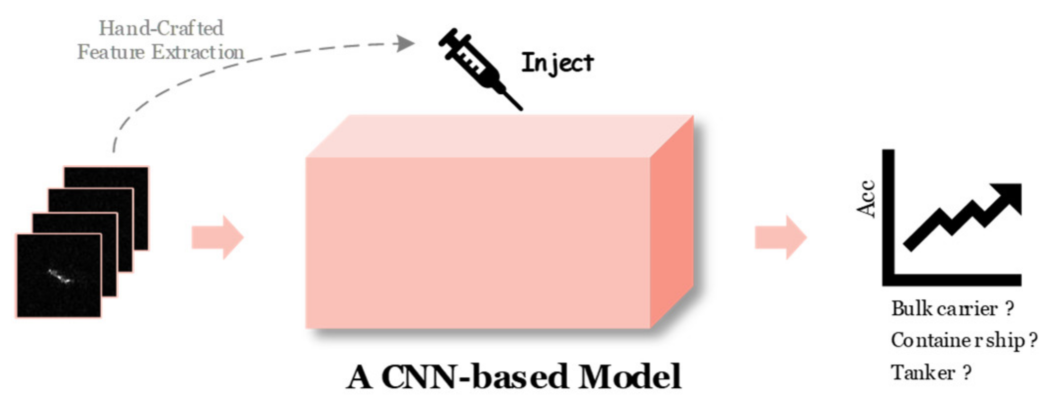
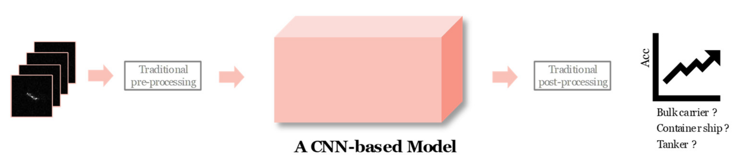
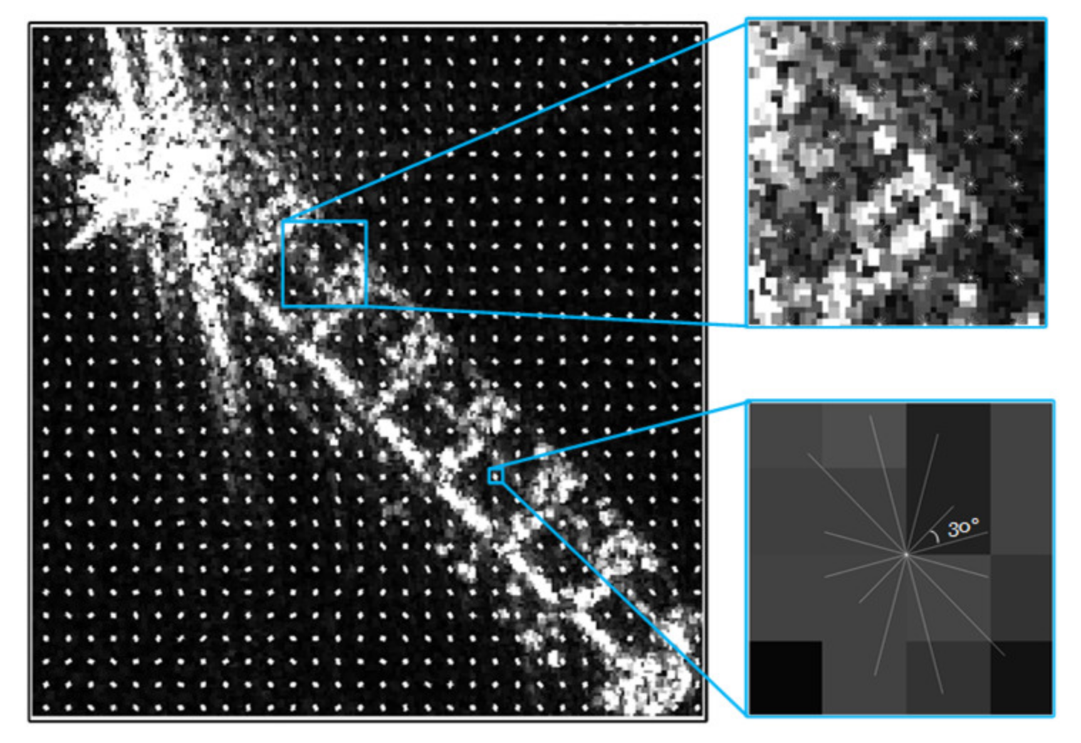
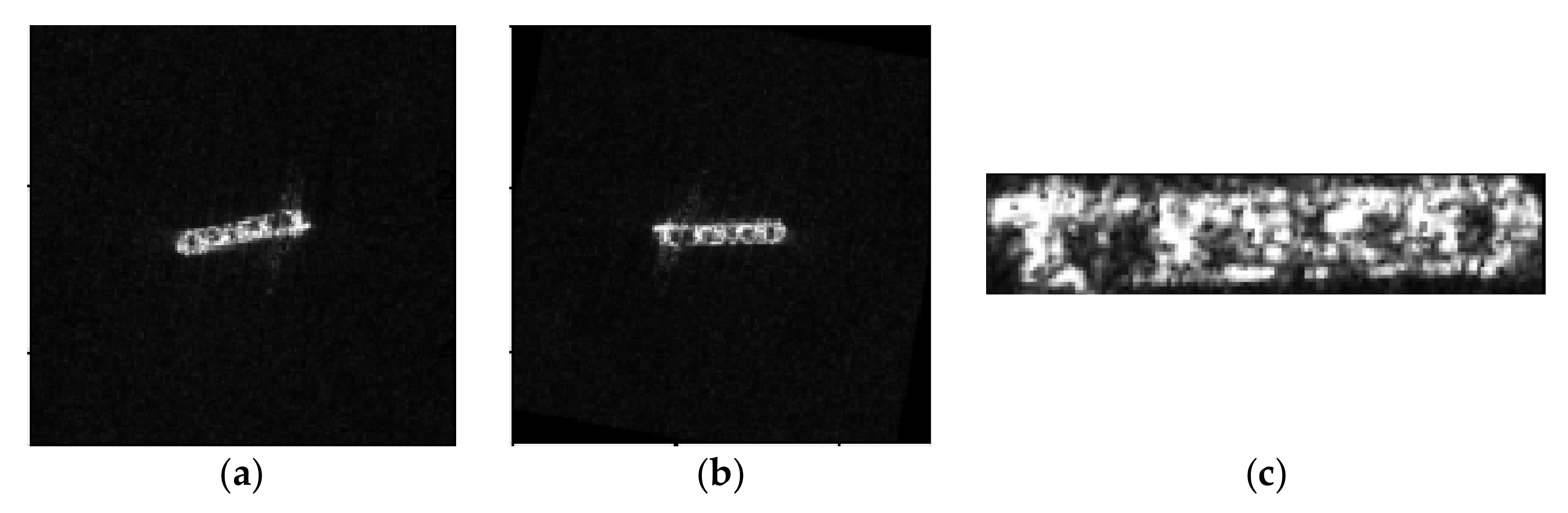
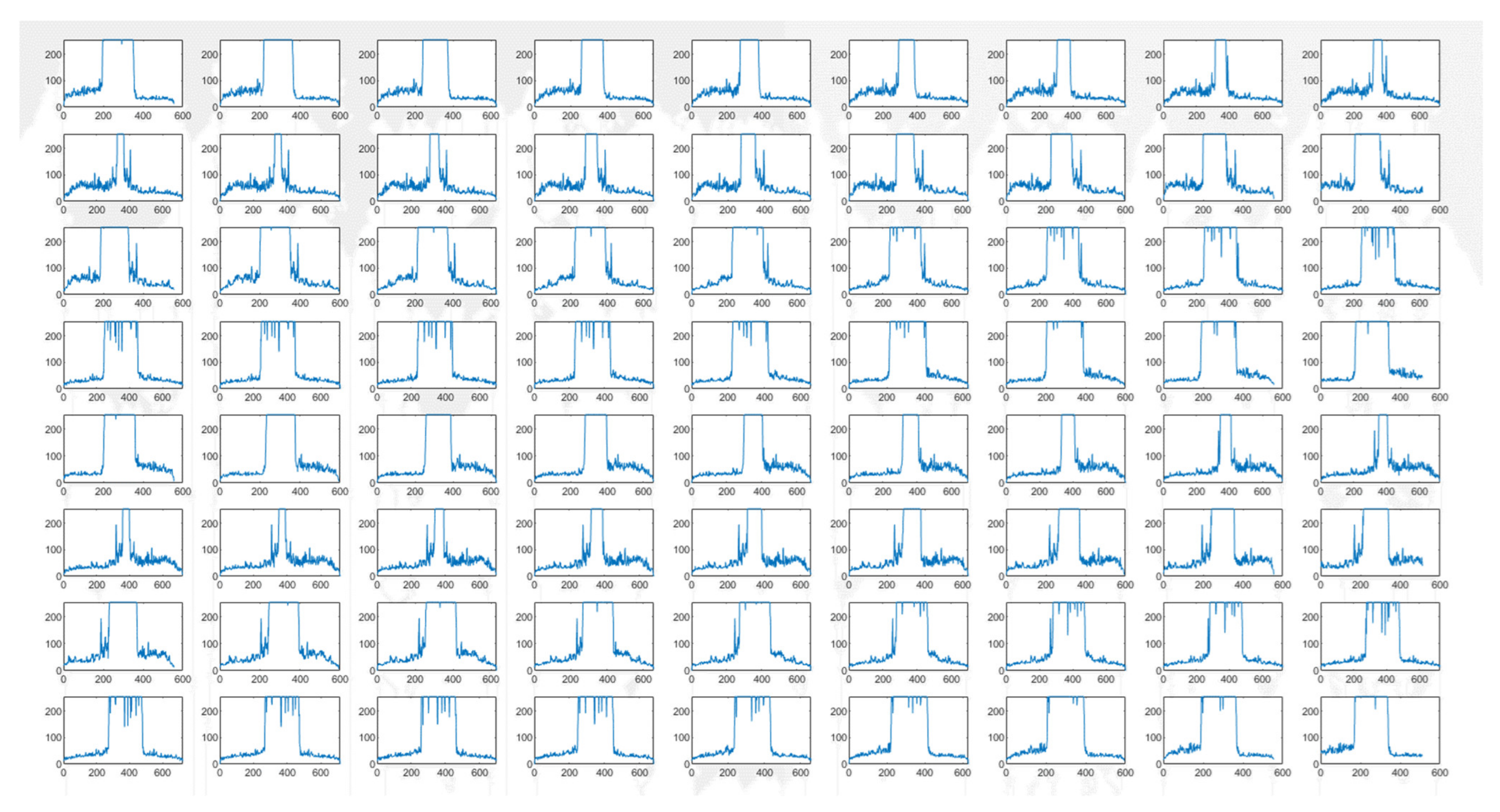
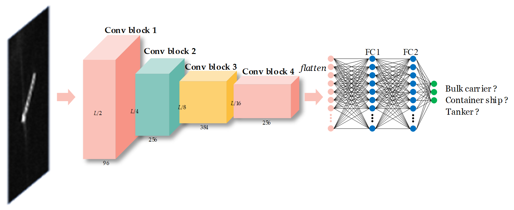
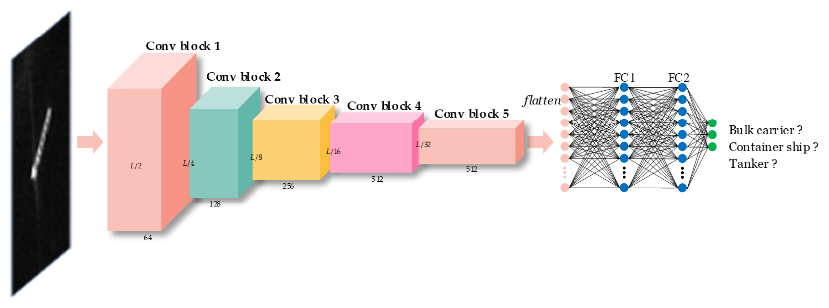
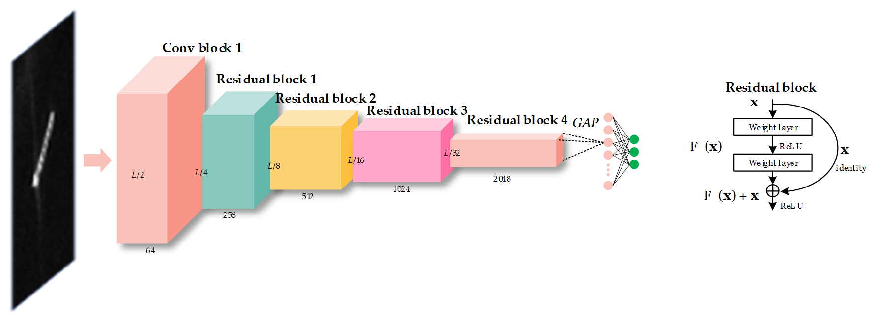
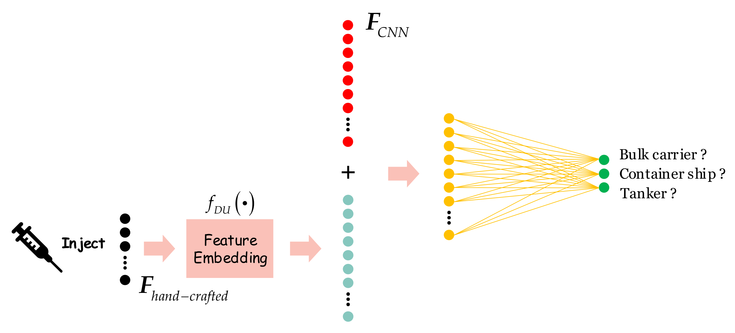
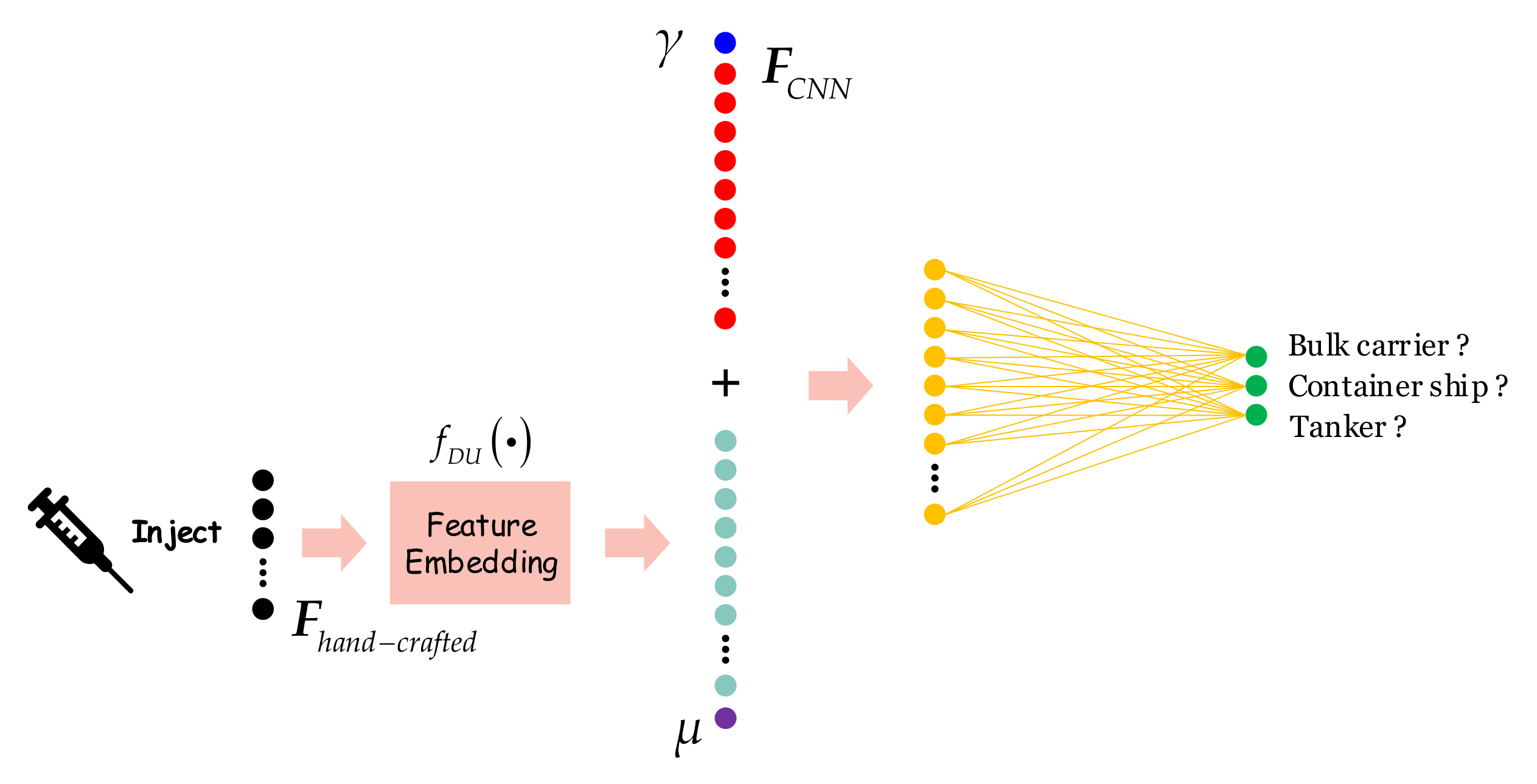
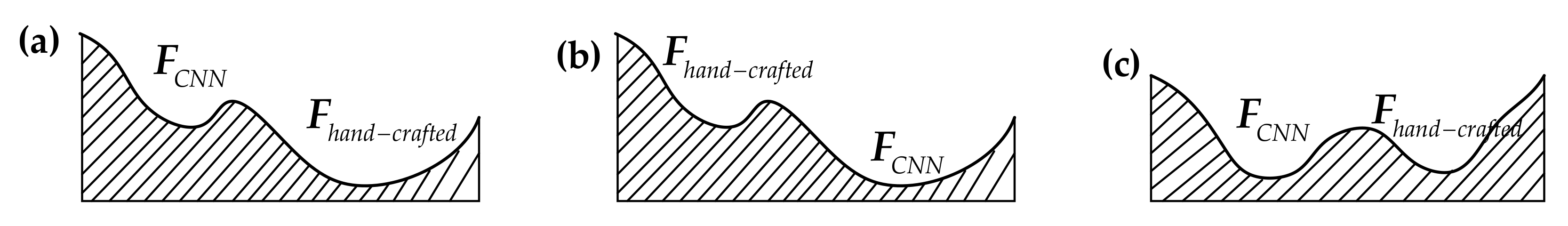
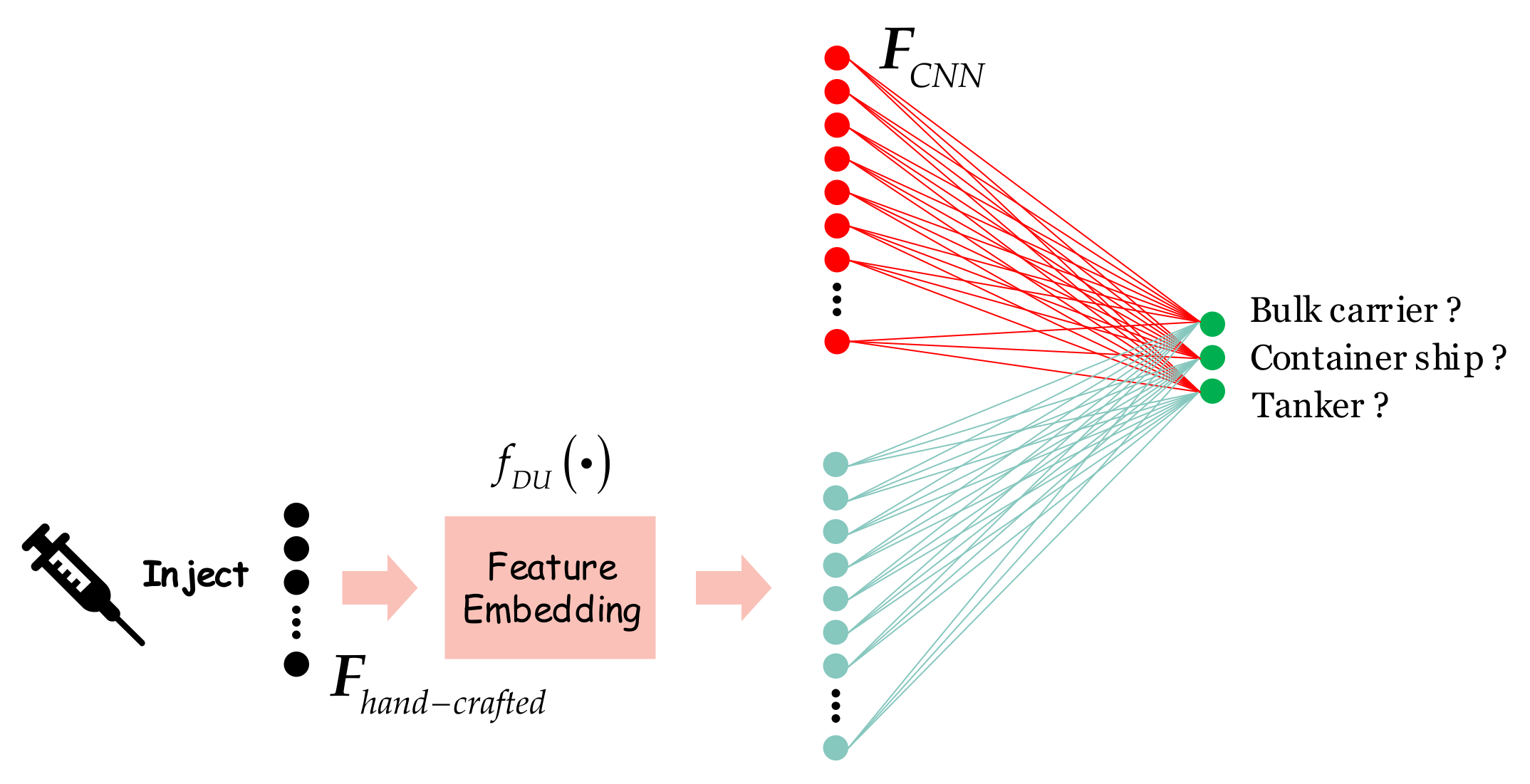
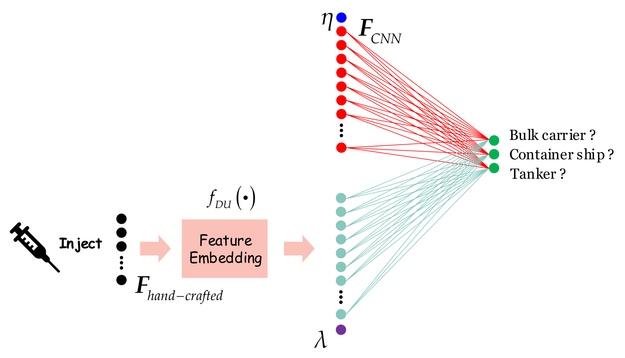
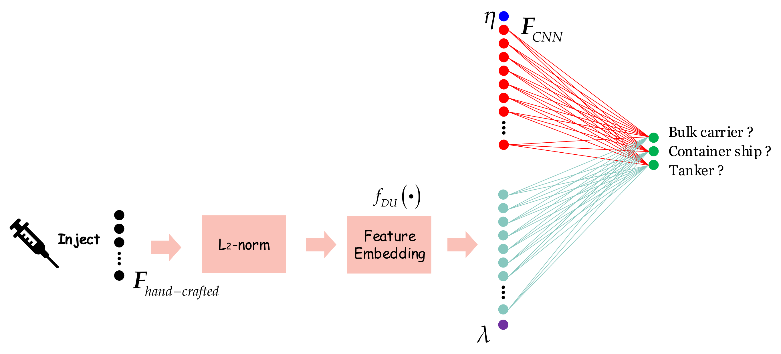
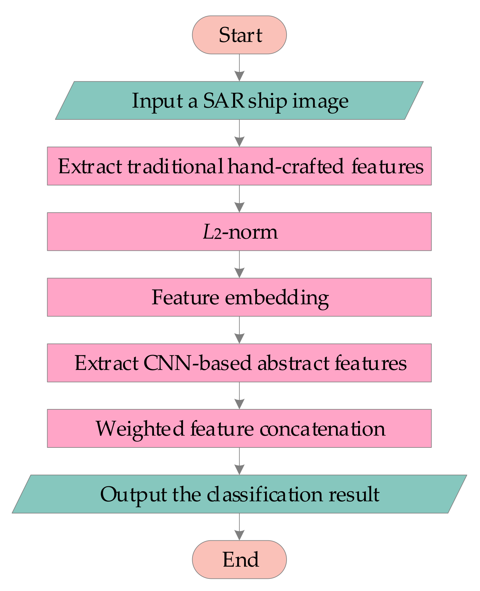
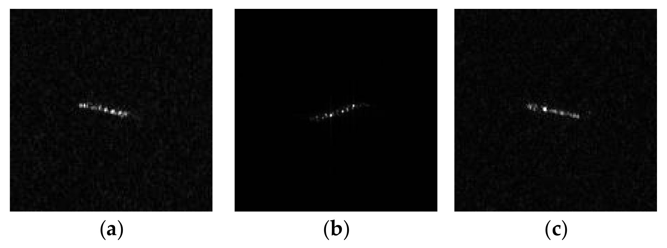
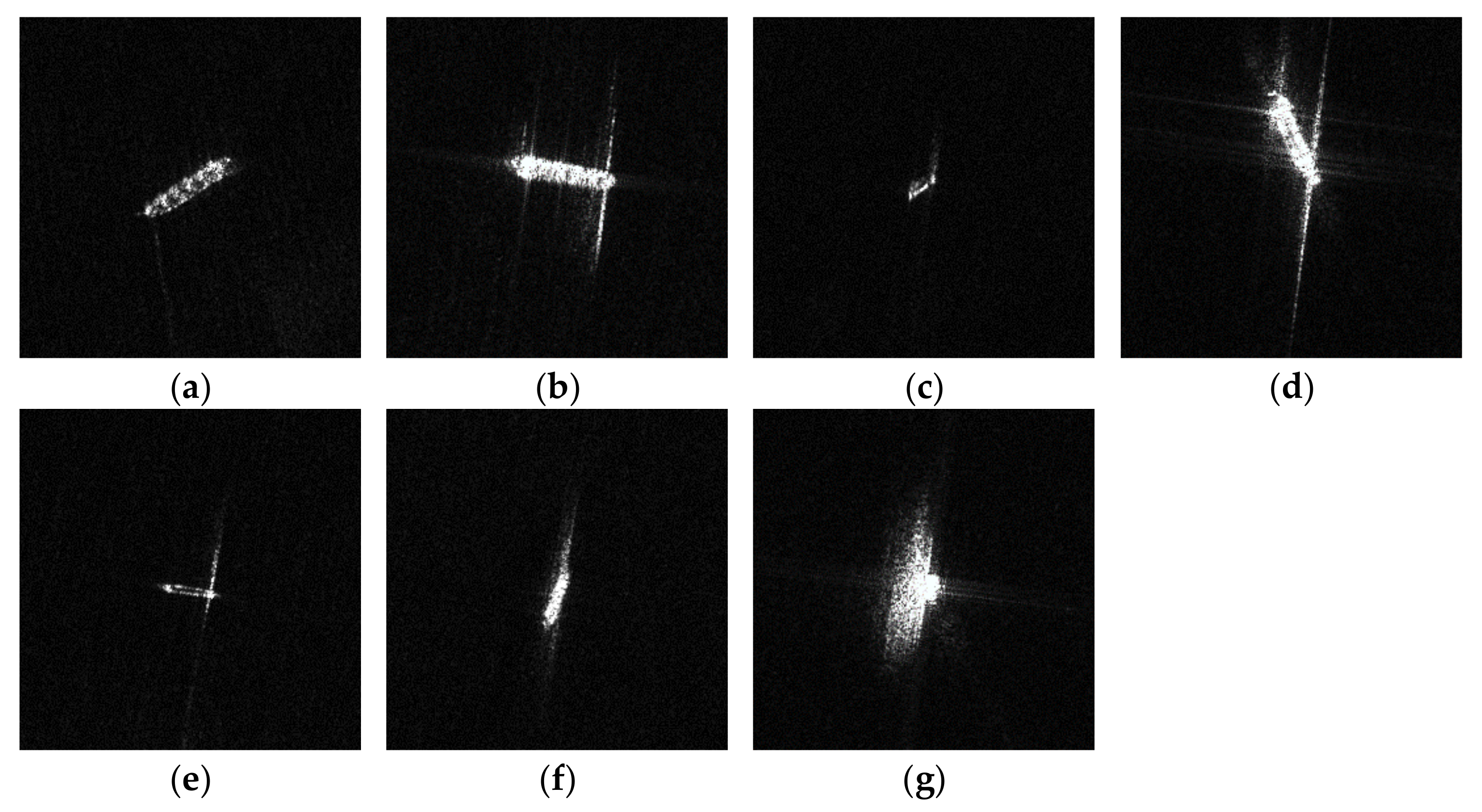
Table 1.
Definition of NGFs. The length (L) and width (W) are both measured by pixel numbers.
| NGFs | Definition | Description |
|---|---|---|
| L | Length | |
| W | Width | |
| 2 × (L + W) | Naive perimeter | |
| L × W | Naive area | |
| L/W | Aspect ratio (a) | |
| W/L | Aspect ratio (b) | |
| (L + W)2/(L × W) | Shape complex | |
| W2/(L2 + W2) | / | |
| (L − W)/(L + W) | / | |
| L/(L + W) | / | |
| W/(L + W) | / |
Table 2.
Training and test set of the OpenSARShip-1.0 dataset.
| Category | Training | Test | All |
|---|---|---|---|
| Bulk carrier | 338 | 328 | 666 |
| Container ship | 338 | 808 | 1146 |
| Tanker | 338 | 146 | 484 |
Table 3.
Training and test set of the FUSAR-Ship dataset.
| Category | Training | Test | All |
|---|---|---|---|
| Bulk carrier | 1150 | 494 | 1644 |
| Container ship | 1219 | 523 | 1742 |
| Fishing | 1101 | 473 | 1574 |
| Tanker | 1215 | 521 | 1736 |
| General cargo | 1205 | 517 | 1722 |
| Other cargo | 1214 | 521 | 1735 |
| Other | 1211 | 520 | 1731 |
Table 4.
SAR ship classification results on the OpenSARShip-1.0 dataset with and without injection.
| CNN Model | Injection Feature Type | Acc (%) | Improvement (%) | Improvement Remarks |
|---|---|---|---|---|
| AlexNet | ✗ | 70.05 | - | - |
| HOG | 74.02 | 3.97 | Avg = 4.29% Max − Min = 2.11% | |
| NGFs | 73.40 | 3.35 | ||
| LRCS | 75.51 | 5.46 | ||
| PAFs | 74.41 | 4.36 | ||
| VGGNet | ✗ | 70.51 | - | - |
| HOG | 76.76 | 6.25 1 | Avg = 5.55% Max − Min = 1.56% | |
| NGFs | 75.20 | 4.69 | ||
| LRCS | 76.44 | 5.93 | ||
| PAFs | 75.83 | 5.32 | ||
| ResNet | ✗ | 72.54 | - | - |
| HOG | 75.43 | 2.89 | Avg = 3.46% Max − Min = 1.09% | |
| NGFs | 76.13 | 3.59 | ||
| LRCS | 75.90 | 3.36 | ||
| PAFs | 76.52 | 3.98 | ||
| DenseNet | ✗ | 74.96 | - | - |
| HOG | 76.83 | 1.87 | Avg = 2.09% Max − Min = 1.63% | |
| NGFs | 76.99 | 2.03 | ||
| LRCS | 78.00 | 3.04 | ||
| PAFs | 76.37 | 1.41 |
1 The maximum accuracy improvement on the OpenSARShip-1.0 dataset is 6.25% (VGGNet + HOG), where only the proposed injection technique is used, without extra processing means.
Table 5.
SAR ship classification results on the FUSAR-Ship dataset with and without injection.
| CNN Model | Injection Feature Type | Acc (%) | Improvement (%) | Improvement Remarks |
|---|---|---|---|---|
| AlexNet | ✗ | 77.42 | - | - |
| HOG | 82.38 | 4.96 | Avg = 5.44% Max − Min = 1.79% | |
| NGFs | 82.46 | 5.04 | ||
| LRCS | 84.17 | 6.75 1 | ||
| PAFs | 82.43 | 5.01 | ||
| VGGNet | ✗ | 80.75 | - | - |
| HOG | 84.79 | 4.04 | Avg = 3.95% Max − Min = 2.53% | |
| NGFs | 84.70 | 3.95 | ||
| LRCS | 83.38 | 2.63 | ||
| PAFs | 85.91 | 5.16 | ||
| ResNet | ✗ | 81.20 | - | - |
| HOG | 85.57 | 4.37 | Avg = 4.20% Max − Min = 1.76% | |
| NGFs | 86.21 | 5.01 | ||
| LRCS | 85.35 | 4.15 | ||
| PAFs | 84.45 | 3.25 | ||
| DenseNet | ✗ | 84.14 | - | - |
| HOG | 86.21 | 2.07 | Avg = 1.87% Max − Min = 1.54% | |
| NGFs | 85.32 | 1.18 | ||
| LRCS | 86.86 | 2.72 | ||
| PAFs | 85.65 | 1.51 |
1 The maximum accuracy improvement on the FUSAR-Ship dataset is 6.75% (AlexNet + LRCS), where only the proposed injection technique is used, without extra processing means.
Table 6.
SAR ship classification results on the OpenSARShip-1.0 and FUSAR-Ship datasets with pure traditional hand-crafted features based on SVM.
Table 6.
SAR ship classification results on the OpenSARShip-1.0 and FUSAR-Ship datasets with pure traditional hand-crafted features based on SVM.
| Dataset | Feature Type | Acc (%) |
|---|---|---|
| OpenSARShip-1.0 | HOG | 66.07 |
| NGFs | 69.81 | |
| LRCS | 67.47 | |
| PAFs | 59.91 | |
| FUSAR-Ship | HOG | 73.05 |
| NGFs | 78.62 | |
| LRCS | 71.36 | |
| PAFs | 69.74 |
Table 7.
Classification confusion matrix of ResNet on the OpenSARShip-1.0 dataset.
| Predicte | Bulk Carrier | Container Ship | Tanker | Acc (%) | |
|---|---|---|---|---|---|
| True | |||||
| Bulk carrier | 202 | 93 | 33 | 61.59 | |
| Container ship | 150 | 613 | 45 | 75.87 | |
| Tanker | 17 | 14 | 115 | 78.77 | |
Table 8.
Classification confusion matrix of ResNet + HOG on the OpenSARShip-1.0 dataset.
| Predicte | Bulk Carrier | Container Ship | Tanker | Acc (%) | |
|---|---|---|---|---|---|
| True | |||||
| Bulk carrier | 204 | 88 | 36 | 62.20 | |
| Container ship | 122 | 643 | 43 | 79.58 | |
| Tanker | 12 | 14 | 120 | 82.19 | |
Table 9.
Classification confusion matrix of ResNet on the FUSAR-Ship dataset.
| Predicte | Bulk Carrier | Container Ship | Fishing | General Cargo | Other | Other Cargo | Tanker | Acc (%) | |
|---|---|---|---|---|---|---|---|---|---|
| True | |||||||||
| Bulk carrier | 451 | 19 | 0 | 10 | 10 | 4 | 0 | 91.30 | |
| Container ship | 16 | 463 | 6 | 14 | 8 | 3 | 13 | 88.53 | |
| Fishing | 8 | 2 | 391 | 0 | 32 | 34 | 6 | 82.66 | |
| General cargo | 28 | 21 | 0 | 437 | 4 | 3 | 24 | 84.53 | |
| Other | 14 | 3 | 69 | 1 | 331 | 78 | 25 | 63.53 | |
| Other cargo | 5 | 3 | 44 | 0 | 50 | 382 | 36 | 73.46 | |
| Tanker | 2 | 11 | 9 | 8 | 14 | 34 | 443 | 85.03 | |
Table 10.
Classification confusion matrix of ResNet + HOG on the FUSAR-Ship dataset.
| Predicte | Bulk Carrier | Container Ship | Fishing | General Cargo | Other | Other Cargo | Tanker | Acc (%) | |
|---|---|---|---|---|---|---|---|---|---|
| True | |||||||||
| Bulk carrier | 453 | 8 | 5 | 7 | 2 | 1 | 18 | 91.70 | |
| Container ship | 9 | 501 | 4 | 1 | 2 | 5 | 1 | 95.79 | |
| Fishing | 2 | 3 | 358 | 0 | 61 | 35 | 14 | 75.69 | |
| General cargo | 6 | 0 | 0 | 499 | 8 | 1 | 3 | 96.52 | |
| Other | 19 | 0 | 81 | 0 | 314 | 66 | 41 | 60.27 | |
| Other cargo | 3 | 0 | 36 | 0 | 21 | 452 | 8 | 86.92 | |
| Tanker | 19 | 6 | 4 | 4 | 9 | 2 | 477 | 91.55 | |
Table 11.
Results of VGGNet + HOG at different injection locations on the OpenSARShip-1.0 dataset.
| Where | Name | Acc (%) | Improve? |
|---|---|---|---|
| Baseline | - | 70.51 | - |
| Location 1 | Conv, Residual, or Dense Blocks | - | - |
| Location 2 | 1D Reshaped CNN-based Features | 69.19 | ✗ |
| Location 3 | Internal FC layer | 68.56 | ✗ |
| Location 4 | Terminal FC layer | 76.76 | ✓ |
Table 12.
Results of VGGNet + HOG with different injection modes on the OpenSARShip-1.0 dataset.
| How | Name | Acc (%) | Improve? |
|---|---|---|---|
| Baseline | - | 70.51 | - |
| Mode 1 | Cat | 74.18 | ✓ |
| Mode 2 | W-Cat | 74.65 | ✓ |
| Mode 3 | DU-Add | 69.66 | ✗ |
| Mode 4 | DUW-Add | 70.44 | ✗ |
| Mode 5 | DU-Cat | 75.12 | ✓ |
| Mode 6 | DUW-Cat | 75.90 | ✓ |
| Mode 7 | DUW-Cat-FN | 76.76 | ✓ |
Publisher’s Note: MDPI stays neutral with regard to jurisdictional claims in published maps and institutional affiliations. |
© 2021 by the authors. Licensee MDPI, Basel, Switzerland. This article is an open access article distributed under the terms and conditions of the Creative Commons Attribution (CC BY) license (https://creativecommons.org/licenses/by/4.0/).
Share and Cite
MDPI and ACS Style
Zhang, T.; Zhang, X. Injection of Traditional Hand-Crafted Features into Modern CNN-Based Models for SAR Ship Classification: What, Why, Where, and How. Remote Sens. 2021, 13, 2091. https://doi.org/10.3390/rs13112091
AMA Style
Zhang T, Zhang X. Injection of Traditional Hand-Crafted Features into Modern CNN-Based Models for SAR Ship Classification: What, Why, Where, and How. Remote Sensing. 2021; 13(11):2091. https://doi.org/10.3390/rs13112091
Chicago/Turabian StyleZhang, Tianwen, and Xiaoling Zhang. 2021. "Injection of Traditional Hand-Crafted Features into Modern CNN-Based Models for SAR Ship Classification: What, Why, Where, and How" Remote Sensing 13, no. 11: 2091. https://doi.org/10.3390/rs13112091
Note that from the first issue of 2016, this journal uses article numbers instead of page numbers. See further details here.