MS-Faster R-CNN: Multi-Stream Backbone for Improved Faster R-CNN Object Detection and Aerial Tracking from UAV Images

Abstract

Tracking objects across multiple video frames is a challenging task due to several difficult issues such as occlusions, background clutter, lighting as well as object and camera view-point variations, which directly affect the object detection. These aspects are even more emphasized when analyzing unmanned aerial vehicles (UAV) based images, where the vehicle movement can also impact the image quality. A common strategy employed to address these issues is to analyze the input images at different scales to obtain as much information as possible to correctly detect and track the objects across video sequences. Following this rationale, in this paper, we introduce a simple yet effective novel multi-stream (MS) architecture, where different kernel sizes are applied to each stream to simulate a multi-scale image analysis. The proposed architecture is then used as backbone for the well-known Faster-R-CNN pipeline, defining a MS-Faster R-CNN object detector that consistently detects objects in video sequences. Subsequently, this detector is jointly used with the Simple Online and Real-time Tracking with a Deep Association Metric (Deep SORT) algorithm to achieve real-time tracking capabilities on UAV images. To assess the presented architecture, extensive experiments were performed on the UMCD, UAVDT, UAV20L, and UAV123 datasets. The presented pipeline achieved state-of-the-art performance, confirming that the proposed multi-stream method can correctly emulate the robust multi-scale image analysis paradigm.

1. Introduction

In recent years, Computer Vision has been involved in several, heterogeneous tasks which include rehabilitation [1,2,3,4,5], virtual/augmented reality [6,7,8,9,10], deception detection [11,12,13,14], robotics [15,16,17,18,19], and much more. Focusing on the latter, one of the most prominent applications involves the usage of drones (hereinafter, UAVs). Their increasing use is related to their low price, making them affordable to a large number of users, and their dimensions, which make them the perfect choice for several tasks. In particular, UAVs do not require a landing strip, they are easy to transport, and they are easy to pilot. These characteristics make UAVs the ideal devices for critical operations such as Search and Rescue (SAR) [20,21,22,23], precision agriculture [24,25,26,27,28], and environmental monitoring [29,30,31,32,33]. Thanks to novel machine learning approaches such as Deep Learning (DL), these tasks can be performed automatically or semi-automatically, with no or little human intervention during the process. However, despite the excellent results obtained with DL, some tasks such as image classification/detection and object tracking need further investigation due to their complexity. For instance, if we consider the object tracking task, the latter is comprised of two stages. The first stage is strictly related to object detection. In fact, the first step of a tracking algorithm is to find the object to track it within the acquired scene. The second stage consists of continuing to find the same object in the subsequent frames.

Usually, tracking is performed in a video surveillance context, thus using static or Pan-Tilt-Zoom (PTZ) cameras that have no or limited camera movements. Moving towards UAVs, this assumption does not hold. With respect to PTZ cameras which have a fixed mounting point, UAVs can move around a target and can change their flight height. In a real use case scenario, e.g., a chase, usually only the change of flight height occurs and the chased object is captured by the same point of view over time (e.g., from behind). In this paper, we propose a novel DL model, namely, the Multi-Stream Faster R-CNN, to provide reliable features at different flight heights for improving tracking by UAVs. A standard Faster R-CNN [34] has, as a backbone, a Convolutional Neural Network (CNN) which extracts features that will be used in both region proposal and classification stages. In the proposed model, the CNN, which is usually based on a visual geometry group (VGG) [35] architecture or a residual neural network (ResNet) [36], is replaced with a multi-stream CNN network. The several streams work, i.e., train and evaluate, in parallel, and they differ on the size of the used kernels, starting from $3\times 3$ up to $7\times 7$. By using this pyramidal approach for the feature extraction process, it is possible to detect objects at different scales. This last aspect creates UAV object detection and tracking the perfect application for the proposed model. Once the object to track has been identified within the scene, the Deep SORT [37] algorithm is used to track it across the frames. Extensive experiments were performed on three state-of-the-art UAV tracking datasets, i.e., UAVDT [38], UAV123 [39], and UAV20L [39]. In addition, to prove the effectiveness of the pyramidal approach, object detection tests were performed on the UMCD dataset [40]. In both tracking and object detection, results line with the state-of-the-art were achieved.

The remainder of this paper is structured as follows. In Section 2, the current literature regarding tracking is discussed. In Section 3, our novel MS Faster R-CNN model is presented. In Section 4, the results obtained in the performed experiments are discussed. Finally, Section 5 concludes the paper.

2. Related Work

The widespread use of machine learning and the always better-performing deep networks let the tracking accuracy increase year after year. Nowadays, the majority of novel proposals are based on variations and different combinations of deep architectures. In general, tracking consists of two important macro phases: the detection of the target(s) and the tracking itself. This section shows some recent approaches dealing with object(s) and/or person(s) detection for tracking purposes. Interested readers can find a recent survey in [41] that explores the problem of tracking and segmentation of objects in video sequences in general, subdividing the proposals by the level of supervision during the learning.

The work in [42] presents a strategy for improving the detection of targets, in this case persons, considering the possible presence of occlusions. The proposal uses an automatic detector to get all the possible targets with a confidence score. After this preliminary phase, a deep alignment network aims at deleting the erroneous bounding boxes. Moreover, the network also extracts appearance features. The results of the network are then combined with a prediction model that, exploiting the previous frames, estimates the more probable target location. All this information is used to create an association cost matrix and the data association is done by the real-time Hungarian algorithm. To handle the occlusions, the strategy relies on the updating of the appearance and motion information frame by frame. If a target in the previous frames cannot be associated with a target in the current frame, then it is taken into account for the next frames considering that an occlusion occurs.

The proposal in [43] estimates the locations of the previously detected targets, in this case persons, by using the Kalman filter combined with temporal information. The temporal information, in the form of tracklets, avoids the decrease of the Kalman filter accuracy in the longterm. Any time a target is detected in the scene, its tracklet is updated and the Kalman filter is reinitialized. In addition, only the confidence score of the last tracklet is taken into account for the final prediction decision. The data association relies on unified scores based on non-maximal suppression. For candidates that have not been associated, they are assigned to the unassigned tracks by using Intersection over Union with a fixed threshold. The other remaining candidates are then discarded.

The detection strategy presented in [44], instead, is applied to vehicle tracking. In this case, the authors rely on the state-of-the-art YOLOv2 detector (presented in [45]), trained on human-annotated frames. The proposed approach exploits the characteristics of the calibrated camera, which allows the backprojection into a 3D space to construct better models. The refinement of detection is based on a bottom-up clustering that fuses together features during the loss computation and relies on histogram-based appearance models to avoid misassignments between nearby targets. At the same time, the network also extracts other useful visual semantic information, such as license plates, type of car, and other deep convolutional features that are then exploited during the tracking.

Moving on to the field of UAV-based tracking, this is increasing its popularity thanks to the decreasing costs of UAVs and the increasing quality of their built-in equipment. However, working with UAV raises different challenges because the perspective of the target in the frames can change even drastically, and also the distance is generally higher, so that the target can occupy only a few pixels of the frame. For this reason, different kinds of approaches have been proposed in literature.

The work in [46] presents a strategy devised for vehicle tracking. The detection step relies on the R-CNN schema, trained on UAV videos. The first part of the strategy consists of the extraction of the feature maps from all the UAV frames by using sharable convolutional layers. The second part deals with the generation of a large number of region proposals on the feature maps created before. This is done by exploiting the region proposal network (RPN) module of the Faster R-CNN network by using a sliding window mechanism. The final part is the training of the RPN and the detector modules with the shared features. Considering that the region proposals are generated by the sliding window mechanism, each of them can be considered as a possible candidate and can also be marked for comparing them during training with labeled data.

The proposal in [47] exploits a multi-level prediction Siamese Network for tracking. The multi-level prediction module aims at identifying the bounding boxes of the targets in the frame. In this module, each prediction level is made up of three parallel branches. The first branch is used to estimate the position of the target, also taking into account the possible motion, while the second branch aims at predicting the target bounding box, and the last one is devised to distinguish between different possible targets in the case of cluttered scenes.

The work in [48] presents a strategy for multi-object tracking based on a novel Hierarchical Deep High-Resolution network. This new network combines the Hierarchical Deep Aggregation network and the High-Resolution Representation network, taking the best properties from them and increasing the computational speed. The network aims at obtaining a multi-scale high-resolution feature representation, which is used to train a prediction network. The quality of the extracted features has been tested feeding three different state-of-the-art networks, namely a CNN, a Cascade R-CNN, and a Hybrid task Cascade. This last one, even if slower with respect to the ordinary CNN, demonstrates the best detection accuracy.

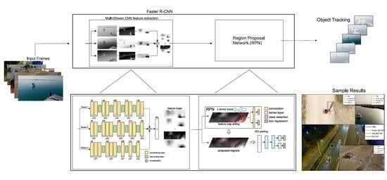
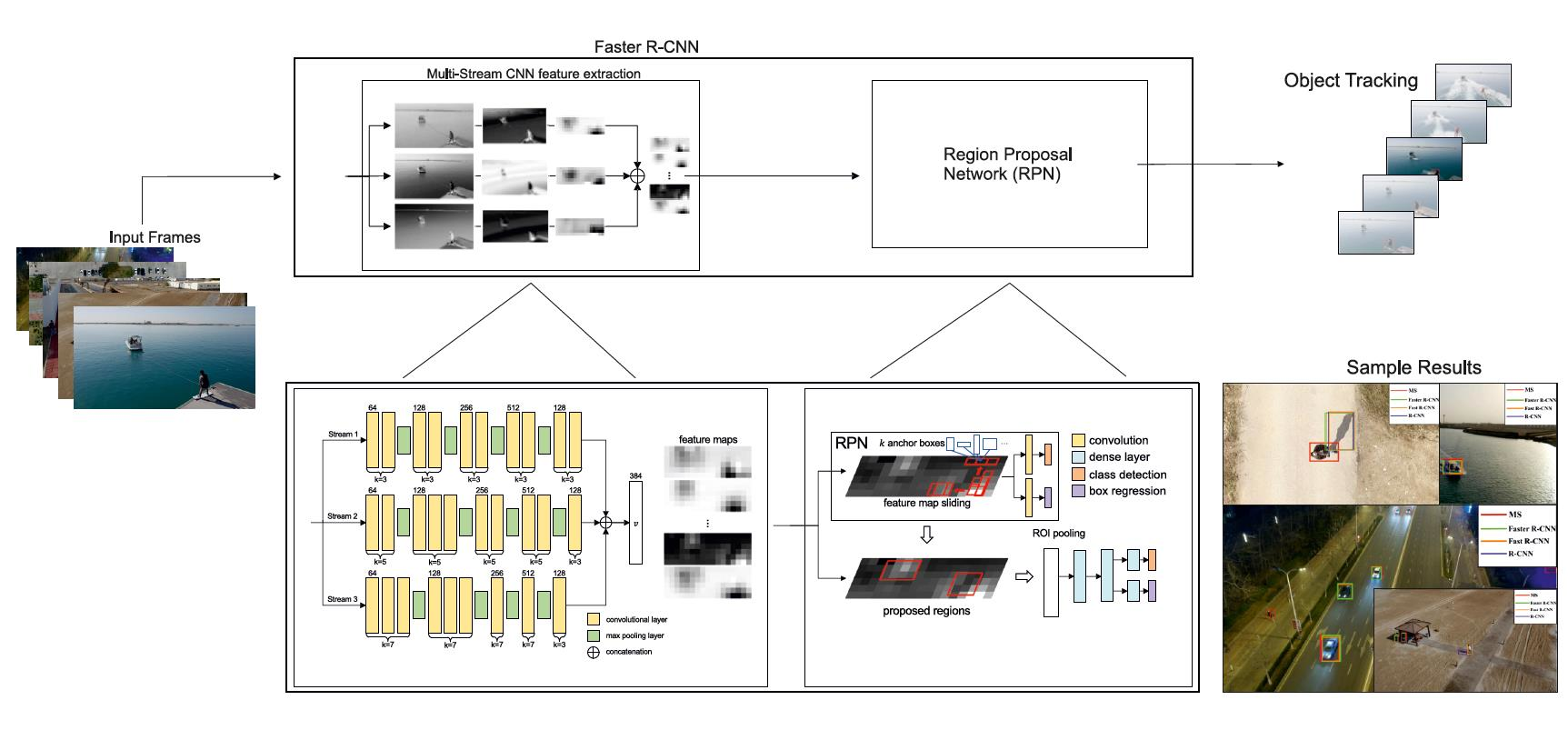
3. Materials and Methods

To correctly track an object across multiple frames of a video sequence, a pipeline composed of three steps is presented in this work. The proposed object tracking approach is summarized in Figure 1. First, a novel Multi-Stream CNN extracts multi-scale features from an object in a given frame, by leveraging its intrinsic architectural design. Second, the extracted feature maps are used to obtain bounding boxes around the objects, according to the Faster R-CNN methodology, where a backbone CNN generates features so that a region proposal network and a region of interest pooling layer can enable a classifier to output the required bounding boxes. Finally, the bounding boxes associated with the various objects are matched together across subsequent frames, according to the Deep SORT [37] tracking algorithm, so that an object can ultimately be followed throughout the video sequence.

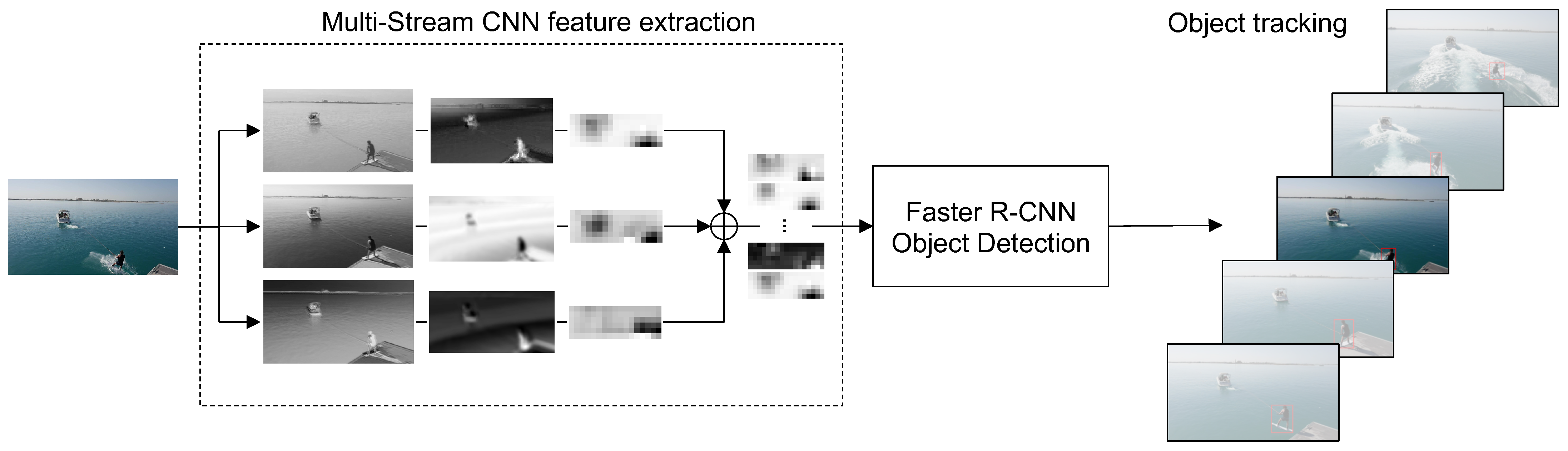
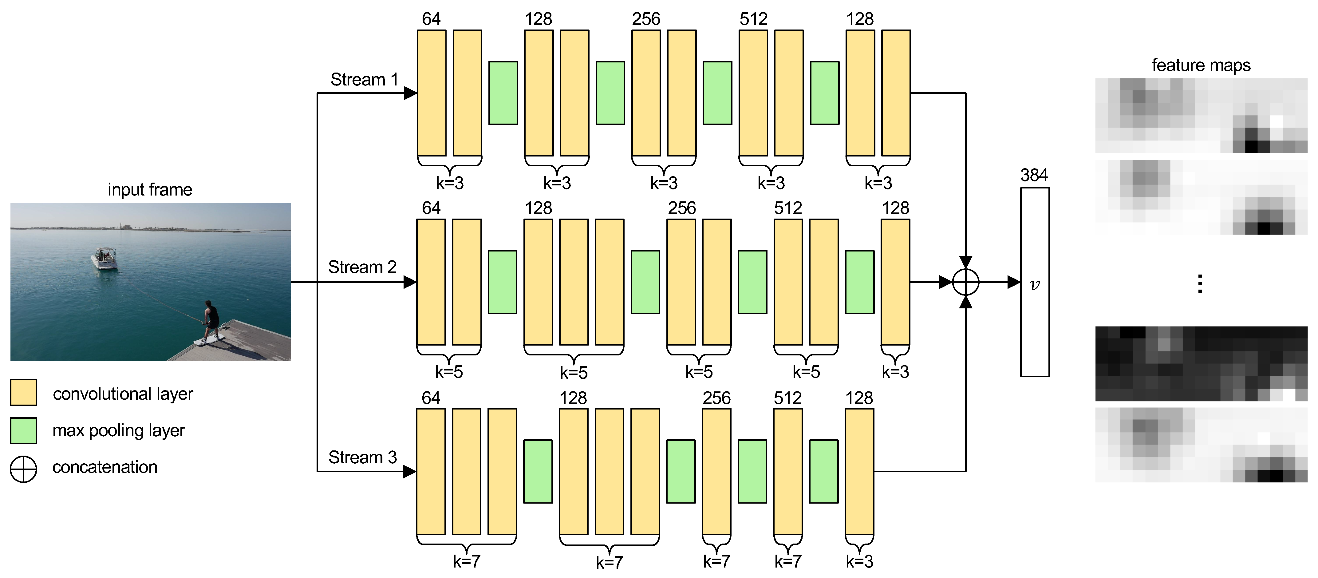
3.1. Multi-Stream CNN Feature Extractor

The core of the proposed approach is the novel multi-stream CNN where the typical image scaling approach, used to learn object characteristics at different scales, is substituted by parallel convolutional streams. Intuitively, given an input image containing an object, each stream analyzes different details by exploiting a specific kernel size during its convolution operations. As a consequence, each filter produced by a specific convolution will capture aspects that would otherwise be missed in a different stream due to the distinct kernel employed—reproducing, to an extent, the multiple-scale input image analysis rationale. As a matter of fact, this behavior can be observed by analyzing the convolution operation. Formally, given an input image I, and a pixel inside this image identified by $I(x,y)$, where x and y correspond to the pixel coordinates; the filtered pixel $f(x,y)$, obtained by applying the kernel, is computed through the following equation:

$$f(x,y)=\omega \ast I(x,y)=\sum _{{\delta }_x=-i}^i\sum _{{\delta }_y=-j}^j\omega ({\delta }_x,{\delta }_y)I(x+{\delta }_x,y+{\delta }_y),$$

(1)

where $\omega$ corresponds to the kernel weights; ${\delta }_x$ and ${\delta }_y$ indicate the x and y coordinates inside the kernel, as well as the neighborhood of the starting pixel, while i=j=$\{3,5,7\}$ represents the kernel size. From (1), it is straightforward to see that, applying multiple convolution operations with different kernel sizes to a given image (i.e., the proposed streams) results in substantially dissimilar output filters due to the employed kernel size differences. An example showing the different kernel size outputs along the three streams is reported in Figure 2.

Concerning the MS CNN implementation, the detailed architecture is resumed in Figure 3. In detail, starting from a resized frame size to maintain the original aspect ratio as well as improve performances, three distinct parallel streams analyze the image through different kernel sizes k to ultimately produce feature maps with equal shape. Specifically, stream 1 contains 10 convolutional layers with kernel size of $3\times 3$, and four max pooling operations are inserted after every pair of convolutions (i.e., after layer 2, 4, 6, and 8). Stream 2 is composed of nine convolutional layers with a kernel shape of $5\times 5$, and a tenth convolution with $k=3$ is employed to reach the correct feature map size. Furthermore, four max pooling layers are inserted after the second, fifth, seventh and ninth convolutional layers to correctly reduce the image size. Lastly, stream 3 includes eight convolutions with kernel size of $7\times 7$, as well as a ninth layer with $k=3$ for the final input reduction, similarly to stream 2. In this case, four max pooling layers are implemented after the third, sixth, seventh and eighth convolutions to, again, reach the correct feature map size. Concerning the number of filters, starting from a size of 64, they are doubled after each max pooling operation (i.e., 64, 128, 256, 512). After the last max pool, instead, a filter bottleneck is applied by implementing convolutions with 128 channels to reduce the number of parameters produced. Finally, since the three streams produce similar sized outputs, the feature maps are concatenated into a single vector representation v, corresponding to the proposed MS CNN backbone output inside the Faster R-CNN pipeline.

3.2. Object Detection

The Faster R-CNN pipeline, summarized in Figure 4, is employed to detect objects inside a given frame. Specifically, starting from feature maps extracted by a backbone CNN, this method first employs a region proposal network to estimate bounding boxes (i.e., proposed regions) and whether or not a specific region contains a relevant object; second, it implements a ROI pooling layer that merges the extracted feature maps with the bounding boxes proposals, and enables a classifier to output both the object class and an appropriate bounding box containing it.

Concerning the RPN component, it creates bounding boxes proposals by sliding a small $n\times n$ window on the extracted features, and mapping them into a lower-dimensional feature vector (i.e., 256). This vector is subsequently fed to two parallel fully-connected layers acting as a box-regressor layer (i.e., $reg$), to encode the bounding boxes center coordinates, width and height, and a box-classification layer (i.e., $cls$), to indicate that a box contains a relevant object. Furthermore, the sliding window generates proposals, called anchors, accounting for several scales and ratios, totalling $k=9$ proposals for each spatial location. Therefore, the $reg$ and $cls$ layers contain $4k$ and $2k$ elements, respectively, while, for each feature map, there will be $W\times H\times k$ proposals, where $W\times H$ correspond to the map size. Notice that, as the original implementation, the sliding window has a size of $n=3$, while $reg$ and $cls$ layers are shared across all spatial locations analyzed by the sliding window to retain the improved performances.

Regarding the ROI pooling and final object detection, starting from the feature maps extracted by the backbone CNN (i.e., the proposed multi-stream network), and the proposals computed by the RPN, an adaptive pooling layer is applied to correctly merge the two inputs into a single vector. Subsequently, the pooled inputs are analyzed through two fully-connected layers, whose output is fed to two siblings classifiers to obtain the final bounding box and object class prediction for the input frame, respectively.

3.3. Multi-Stream Faster R-CNN Loss Functions

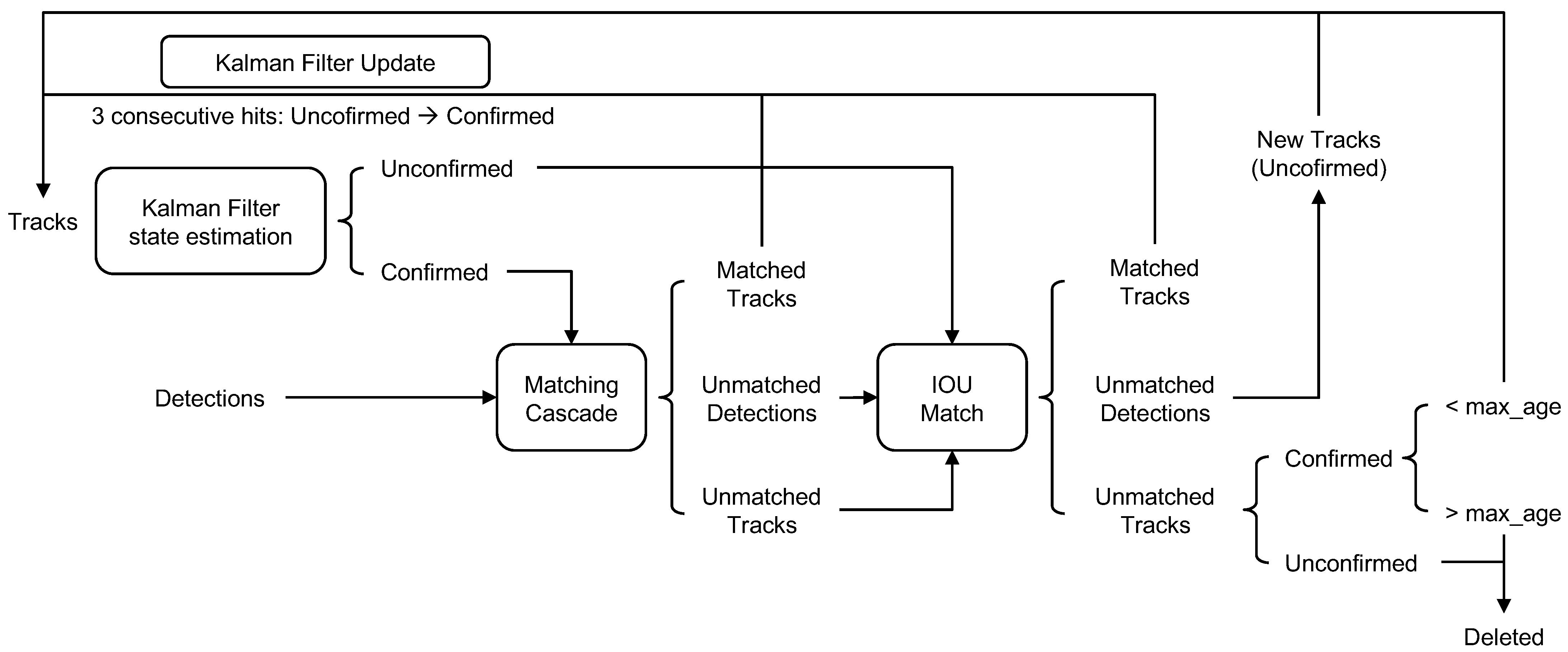
In accordance with [34], the presented methodology can be trained in an end-to-end fashion since, in this work, relevant modifications were only applied to the backbone CNN used to extract features from an input image. More accurately, the Faster R-CNN pipeline employs a multi-task loss function associated with the bounding box regression and object classification tasks. Formally, as per the definition by [34], for a given mini-batch, the function to be minimized is computed according to the following equation:

$$L(\left\{p_i\right\},\left\{t_i\right\})=\frac{1}{N_{cls}}\sum _i{L}_{cls}(p_i,p_i^{\ast })+{\lambda }_l\frac{1}{N_{reg}}\sum _i{p}_i^{\ast }{L}_{reg}(t_i,t_i^{\ast }),$$

(2)

where i indicates the i-th anchor of a mini-batch; $p_i$ and $p_i^{\ast }$ represent the predicted and ground truth probability of the anchor being associated with a relevant object; $t_i$ and $t_i^{\ast }$ are the generated and ground truth vectors containing the parameterized bounding box coordinates (i.e., center x and y, width and height); $N_{cls}$ and $N_{reg}$ correspond to normalization terms based on the batch size and the number of proposed anchors, respectively, while ${\lambda }_l$ is a balancing parameter to ensure both losses have similar weights. Moreover, $L_{cls}$ is a binary cross-entropy loss function, while $L_{reg}$ is a regression loss using the robust function defined in [49], namely:

$$L_{reg}(t_i,t_i^{\ast })=\sum _{i\in \{x,y,w,h\}}{\mathrm{smooth}}_{L_1}(t_i-t_i^{\ast }),$$

(3)

where the smooth function is computed as follows:

$${\mathrm{smooth}}_{L_1}(x)=\left\{\begin{array}{cc}0.5x^2\hfill & \mathrm{if}\left|x\right|<1;\hfill \\ \left|x\right|-0.5\hfill & \mathrm{otherwise}.\hfill \end{array}\right.$$

(4)

Finally, concerning the bounding box regression, we employed the same parameterization defined in [50], described via the following equations:

$$\begin{array}{cc}\hfill & t_{\mathrm{x}}=(x-x_a)/w_a,t_{\mathrm{y}}=(y-y_a)/h_a,\hfill \\ \hfill & t_{\mathrm{w}}=log(w/w_a),t_{\mathrm{h}}=log(h/h_a),\hfill \\ \hfill & t_{\mathrm{x}}^{\ast }=(x^{\ast }-x_a)/w_a,t_{\mathrm{y}}^{\ast }=(y^{\ast }-y_a)/h_a,\hfill \\ \hfill & t_{\mathrm{w}}^{\ast }=log(w^{\ast }/w_a),t_{\mathrm{h}}^{\ast }=log(h^{\ast }/h_a),\hfill \end{array}$$

(5)

where x, y, w, and h correspond to the bounding box center coordinates, width, and height, respectively, while the variables x, $x_a$, and $x^{\ast }$ are associated with the predicted bounding box, proposed anchor bounding box, and ground truth bounding box, respectively. The same reasoning applies to the other parameters (i.e., y, w, and h).

3.4. Tracking

Once the MS Faster R-CNN can correctly detect objects inside a video stream, the Deep SORT [37] algorithm is exploited as is to achieve real-time tracking capabilities from UAV images. Specifically, the Deep SORT procedure exploits visual appearances extrapolated from the bounding boxes, in conjunction with a recursive Kalman filtering and frame-by-frame data association strategy to describe object tracks across a video sequence. The Deep SORT flowchart is summarized in Figure 5.

In detail, a tracked object is described via the 8-dimensional space ($u,v,w,h,\dot{x},\dot{y},\dot{w},\dot{h}$), where u, v, w, and h represent, respectively, the bounding box center coordinates, width and height, while $\dot{x}$, $\dot{y}$, $\dot{w}$, and $\dot{h}$ indicate the corresponding velocities. Moreover, to correctly track an object across multiple frames using this space, the Deep SORT algorithm implements a weighted sum of two distinct metrics inside a matching cascade strategy: the Mahalanobis distance $D_1$, to provide short-term locations predictions based on a given object movement; and the cosine distance $D_2$, to embed appearance information into the tracker and handle long-term occlusions. The association between the current Kalman state and a new measurement is then optimally solved via the Hungarian algorithm, from which the Kalman state is updated for usage in the subsequent frame. To provide a clear overview of how the Hungarian algorithm resolves the assignment problem, its pseudocode for a general assignment problem is provided in Algorithms 1 and 2.

Algorithm 1 Hungarian Algorithm

1: functionHungarian Algorithm 2:     Input: BG = Bipartite Graph {V, U, E}, C = $n\times n$ matrix containing edge costs 3:     Output: M = a complete matching 4:     $M,\alpha ,\beta \leftarrow init()$ 5:     for $i\leftarrow 1,n$ do 6:         $M,\alpha ,\beta \leftarrow stage()$ 7:     end for 8:     return M 9: end function 10:   11:   12: functioninit 13:     Input: BG, C 14:     Output $M,\alpha ,\beta$ 15:     $M\leftarrow \varnothing$ 16:     for $i\leftarrow 1,\left|V\right|$ do 17:         ${\alpha }_i\leftarrow 0$ 18:     end for 19:      20:     for $i\leftarrow 1,\left|U\right|$ do 21:         ${\beta }_i\leftarrow mi{n}_i(c_{ij})$ 22:     end for 23:     return M, $\alpha$, $\beta$ 24: end function

Formally, for a given i-th track and j-th bounding box, the weighted association sum is computed as follows:

$$a_{i,j}={\lambda }_a{D}_1(i,j)+(1-{\lambda }_a)D_2(i,j),$$

(6)

where ${\lambda }_a$ is an hyperparameter regulating the influence of each loss. Finally, the Mahalanobis distance $D_1$ and cosine distance $D_2$ are defined as:

$$\begin{array}{cc}\hfill D_1(i,j)& ={(t_j-z_i)}^{\mathrm{T}}{\mathcal{S}}_i^{-1}(t_j-z_i),\hfill \\ \hfill D_2(i,j)& =min\{(1-r_j^{\mathrm{T}}{r}_k^{(i)}|r_k^{(i)}\in {\mathcal{R}}_k\},\hfill \end{array}$$

(7)

where $t_j$ refers to the j-th bounding box detection; $z_i$ represents the i-th track projection onto the measurement space ${\mathcal{S}}_i$; $r_j$ is an appearance descriptor for the j-th box, while ${\mathcal{R}}_k={\left\{r_k^{(i)}\right\}}_{k=1}^{L_k}$ is a gallery containing the last $L_k$ associated descriptors of every track k.

Algorithm 2 Hungarian Algorithm (continued)

1: functionstage 2:     Input: $M,\alpha ,\beta$, BG, C 3:     Output: $M,\alpha ,\beta$ 4:      5:     for k in each unmatched node in V do 6:         Set k as the root of a Hungarian tree 7:         Create the Hungarian tree rooted in k using the equality subgraph 8:         $I\ast \leftarrow$ each node index from V contained in the tree rooted in k 9:         $J\ast \leftarrow$ each node index from U contained in the tree rooted in k 10:         if ∃ an augmenting path then 11:            $M\leftarrow (M-P)\cup (P-M)$ where P is the set of edges in the augmenting path 12:            break 13:         else 14:            $\theta =\frac{1}{2}mi{n}_{i\in I\ast ,j\in J\ast }(c_{ij}-{\alpha }_i-{\beta }_j)$ 15:            $\alpha \leftarrow$ $\left\{\begin{array}{cc}{\alpha }_i+\theta \hfill & i\in I\ast \hfill \\ {\alpha }_i-\theta \hfill & i\notin I\ast \hfill \end{array}\right.$ 16:            $\beta \leftarrow$ $\left\{\begin{array}{cc}{\beta }_i-\theta \hfill & j\in J\ast \hfill \\ {\beta }_i+\theta \hfill & j\notin J\ast \end{array}\right.$ 17:         end if 18:     end for 19:     return $M,\alpha ,\beta$ 20: end function

4. Experimental Results

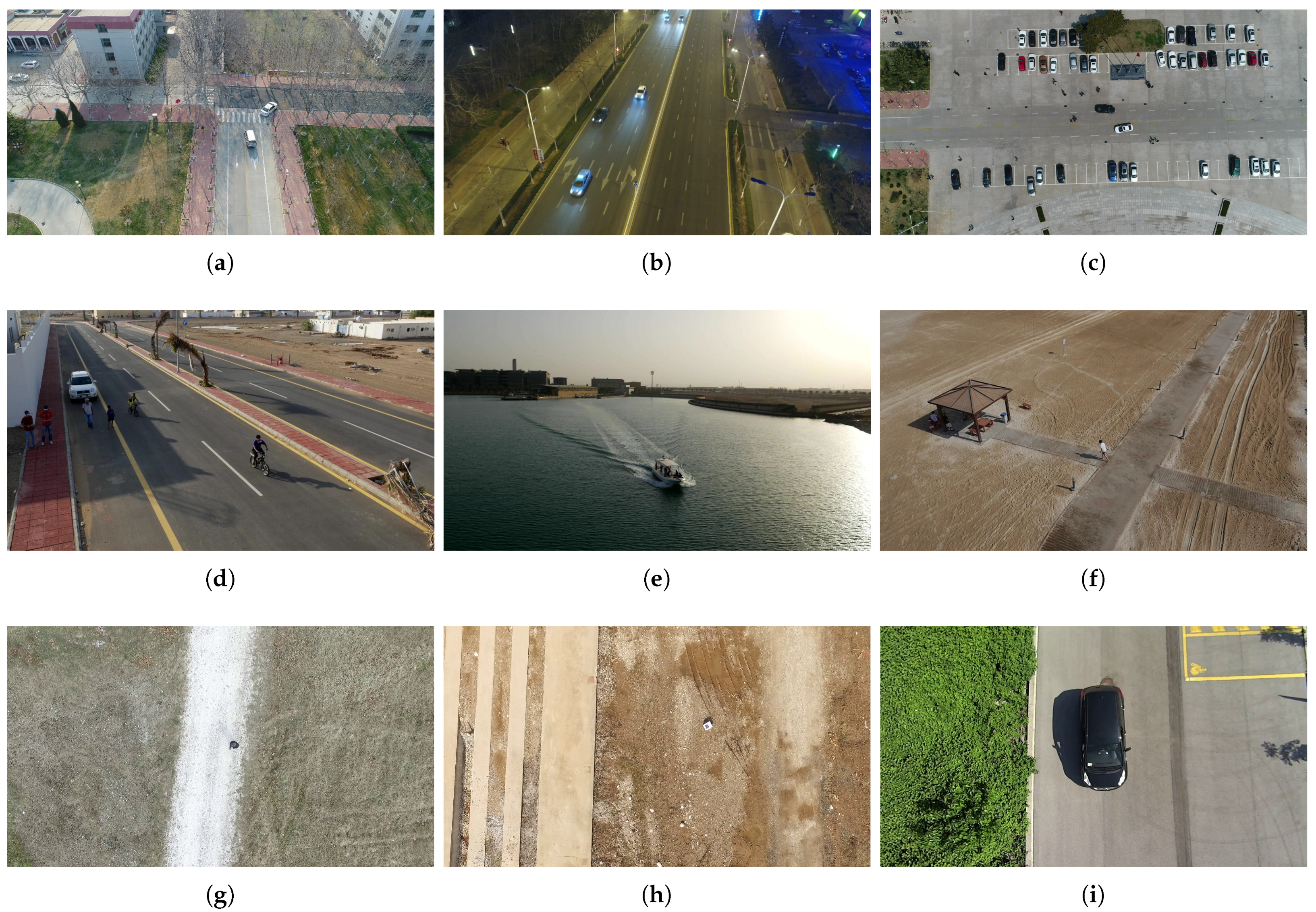
This section presents the results obtained with the proposed MS model in both object detection and tracking. Firstly, the used datasets are described. Secondly, implementation details, together with the obtained results, are discussed.

4.1. Datasets

The data used for this work was taken from four well-known benchmarks in UAV object detection and tracking, namely UMCD [40], UAVDT [38], UAV123 [39], and UAV20L [39] captured on UAV platforms. A total number of 273 sequences was used, which consists of more than 190,000 frames specifically designed for three of the most important tasks of Computer Vision like object detection, single object tracking, and multiple object tracking. The data are also rich in task specific attributes that give the possibility to experiment in different conditions like different altitudes, occlusion, camera motion, background clutter, and more.

4.1.1. UAVDT

The UAVDT dataset is a benchmark dataset focused on complex scenarios containing 100 sequences with more than 80,000 frames for three fundamental Computer Vision tasks: Object Detection (DET), single object tracking (SOT), and multiple object tracking (MOT). This UAV dataset represents 14 kinds of different task based attributes. For DET tasks, the defined attributes are three: vehicle-category, vehicle-occlusion, and out-of-view. In case of MOT, there are also three defined attributes, namely weather condition (WC), flying altitude (FA) and camera view (CW). Finally, for SOT, there are eight defined attributes: background clutter (BC), camera rotation (CR), Object rotation (OR), small object (SO), illumination variation (IV), object blur (OB), scale variation (SV), and large occlusion (LO).

4.1.2. UAV123 and UAV20L

The UAV123 is a benchmark dataset for low altitude UAV target tracking. The dataset comes with 123 video sequences and more than 110,000 frames suitable for short-term tracking and also for long-term tracking (UAV20L). Based on their characteristics, videos are organized in nine attributes such as: aspect ratio change (ARC), background clutter (BC), camera motion (CM), fast motion (FM), full occlusion (FO), illumination variation (IV), low resolution (LR), out-of-view (OV), partial occlusion (POC), similar object (SO), scale variation (SV), and viewpoint change (VC).

4.1.3. UMCD

The UMCD is a recently released dataset used for testing UAV mosaicking and change detection algorithms. It is comprised of 50 challenging videos acquired at very low altitudes, i.e., between 6 and 15 m, on different environments, such as dirt, countryside, and urban. The dataset contains several objects within the several scenes, e.g., persons (both single and in group), cars, boxes, suitcases, and more. These characteristics make this dataset the ideal choice for testing the proposed model on the object detection task from UAV.

To provide a better overview of the used datasets, their main characteristics are resumed in

Table 1. Summary table of the exploited datasets.

Dataset	Task (s)	# Sequences	#Frames (Approx)
UAVDT [38]	Object Detection Single Object Tracking Multiple Object Tracking	100	80,000
UAV123 [39] UAV20L [39]	Short-Term Tracking Long-Term Tracking	123	110,000
UMCD [40]	Object Detection (Very Low Altitudes)	50 (challenging)	48,765
Used in this work	Object Detection Object Tracking	273	more than 190,000

, while samples taken from each collection are reported in Figure 6. As shown, each dataset presents several unique features that allow for exhaustively testing UAV tracking algorithms.

4.2. Evaluation Metrics

Concerning the object detection task, the standard mean Average Precision (mAP) is used, and only the frames in which an object is fully visible are considered.

Regarding the tracking task, we use Precision and Success Rate as metrics for quantitative analysis of the performance based on the one-pass evaluation (OPE) process. This evaluation method consists of running trackers throughout a test sequence with initialization from the manually annotated ground-truth position in the first frame and reporting the precision plot or the success rate plot. The tracking precision is calculated in each frame by the center location error (CLE), which is defined as the Euclidean distance between the center location of the tracked target and the manually labeled ground truth. The precision plot measures the overall performance of the tracker by showing the percentage of frames whose estimated CLE is within a given maximum threshold. Success rate for trackers is measured by the bounding box overlap. Given the tracked bounding box $R_T$ and the manually annotated bounding box $R_G$, the success rate is calculated as the intersection over union of $R_T$ and $R_T$ as follows:

$$\mathrm{IoU}=\frac{|{\mathbf{R}}_T\cap {\mathbf{R}}_G|}{|{\mathbf{R}}_T\cup {\mathbf{R}}_G|}$$

(8)

To measure the overall performance on a sequence of frames, the number of successful frames where IoU is higher than a given maximum threshold is counted and the success rate plot is used to show the percentage or the ratio of successful frames. The final score is calculated as the AUC to represent the overall tracking performance based on success rate.

4.3. Implementation Details

Considering the used framework and hardware, the proposed method is implemented in Pytorch [51], and the machine used for the experiments consisted of a AMD Ryzen 1700 processor, 16 GB DDR4 RAM, a 500 GB solid state disk, and an Nvidia RTX 2080 GPU. As hyper-parameters, a learning rate of 0.001, together with AdamW optimizer, were used.

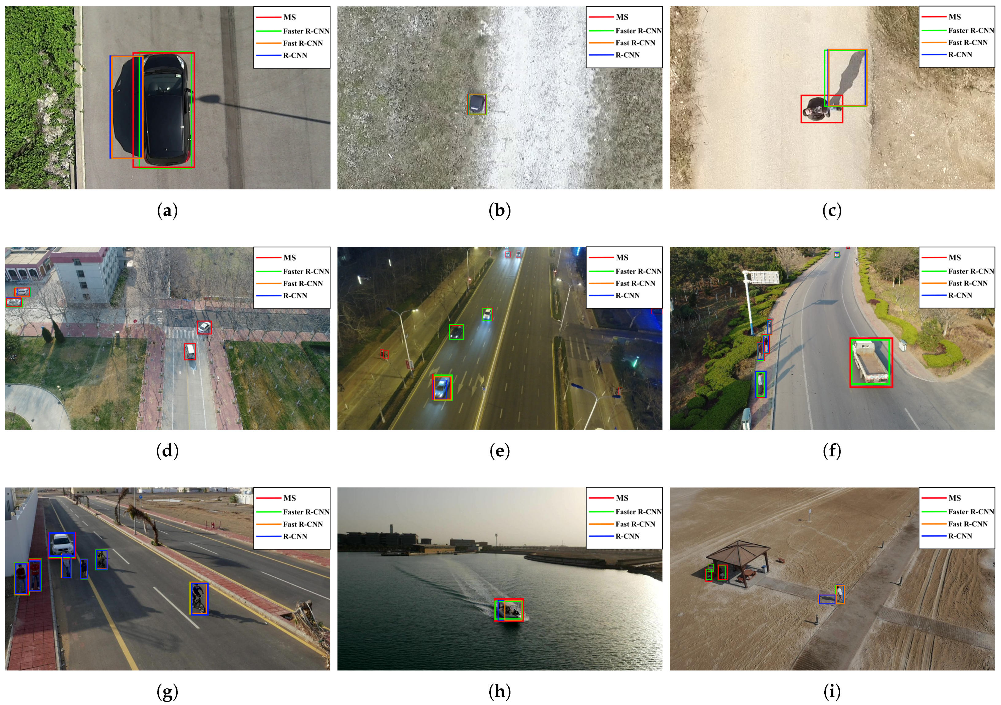
4.4. Object Detection Performance Evaluation

For the object detection task, the proposed model was compared with the standard Faster R-CNN. Both of the models were fine-tuned on the object classes contained inside the UMCD dataset. This step was necessary since some classes, such as tires, bags, suitcases, and so on, are not present within the datasets on which well-known models are usually pre-trained (e.g., VOC, ImageNet, etc.). Even in the case that the class is present, it is not acquired from a UAV perspective, hence an object may be easily misclassified. In Figure 7, some examples of object detection on the UMCD dataset are shown. While in Figure 7a,b the two models perform very similarly, it is noticeable that, in Figure 7c, MS overcomes the standard Faster R-CNN. As it is possible to see, the latter detects the shadow of the person as the person itself. Concerning the overall performance, we obtained a mAP of $97.3\%$ with MS and a mAP of $95.6\%$ with Faster R-CNN on the used dataset. Since the objects present within the videos are acquired by using a Nadir view, the proposed pyramidal approach allows the extraction of more reliable feature vectors.

In addition, to provide a complete overview concerning the object detection, further experiments were performed using different R-CNN models and datasets. In detail, for the former, we added to our comparisons the base R-CNN [50] and the Fast R-CNN [49], while, for the latter, we have used UAV123 and UAVDT again. Notice that these two datasets are not as challenging as the UMCD for the object detection task. This is mainly due to the fact that all the objects in the UMCD collection are acquired with a Nadir view, thus making it difficult to detect objects especially at higher flight altitudes. In fact, in some images, the elements present within the scene have a silhouette as if they were acquired by a standard static camera. This means that it is easier to perform their detection with well-known object detectors. This fact is noticeable from Figure 7d–i, where only the proposed model correctly detects the elements within the analyzed scene.

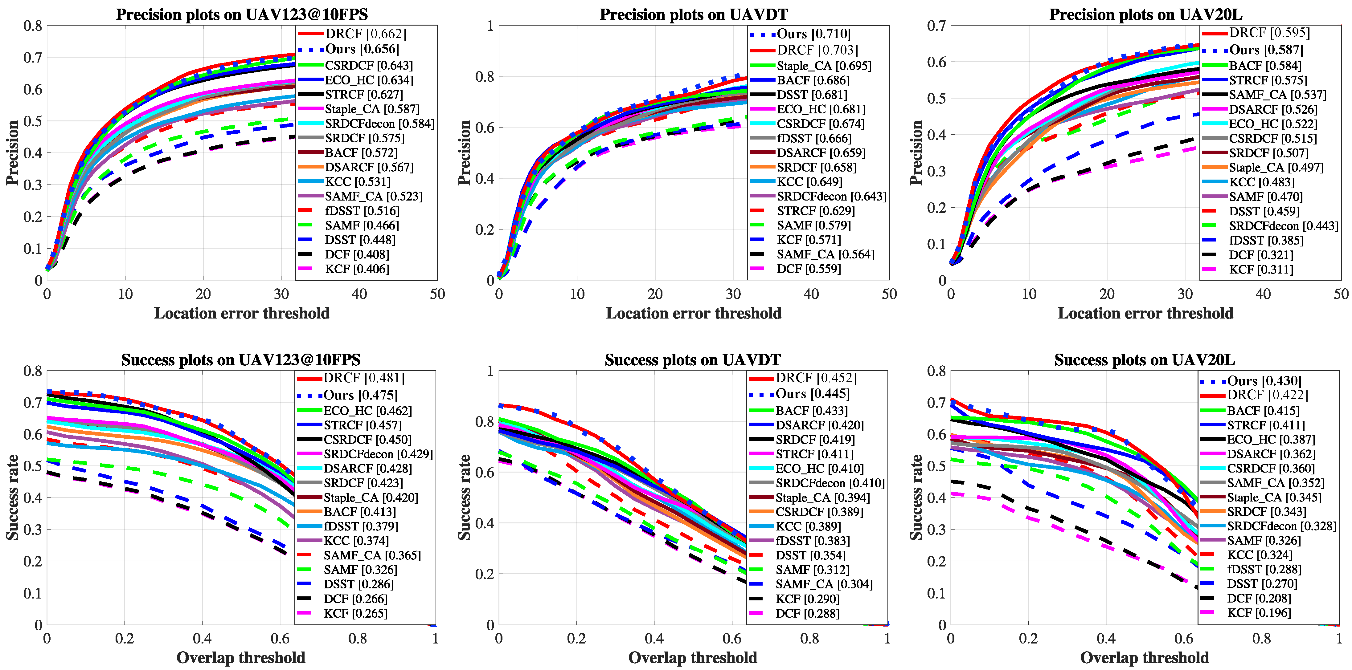
4.5. Tracking Performance Evaluation

The proposed method is compared with 16 state-of-the-art deep-based trackers. These trackers are, namely, DSARCF [52], ECO-HC [53], CSRDCF [54], STRCF [54], Staple_CA [55], SRDCF [56], SRDCFdecon [57], BACF [58], KCC [59], SAMF_CA [55], fDSST [60], SAMF [61], DSST [62], KCF [63], DCF [63], and DRCF [64]. As mentioned in Section 4.2, the trackers are evaluated with the AUC on the Success Plot and the CLE for the Precision plot. For the latter, the common 20 pixels threshold is used.

Precision and Success plots are shown in Figure 8. It is possible to observe that the proposed method is in line with the current state-of-the-art in both plots. More specifically, MS (i.e., “Ours” in the plots) outperforms all the methods in the UAVDT precision plot by achieving a precision of $0.710$, followed by DRCF (0.703) and Staple_CA(0.695). This is again thanks to the MS pyramidal approach that allows for correctly handling the several altitudes, i.e., low (10–30 m), medium (30–70 m) and high (>70 m), of the UAVDT dataset. Concerning UAV123 and UAV20L precision plots, MS is places in the second position with a precision of $0.656$ and $0.587$, respectively, following DRCF in both cases ($0.662$ and $0.595$) and followed by CSRDCF ($0.643$) in the UAV123 dataset and BACF ($0.584$) in the UAV20L dataset.

Regarding the success plots, MS overcomes the competitors on the UAV20L dataset. In detail, it achieves a success rate of $0.430$, followed by DRCF ($0.422$) and BACF ($0.415$). Instead, on UAV123 and UAVDT, the proposed MS model is the second best tracker with a success rate of $0.475$ and $0.445$, respectively, following DRCF with scores of $0.481$ and $0.452$, respectively. These success plots highlighted that our model is the best for tracking an object in long sequences. This is amenable to the pyramidal feature extraction that allows for better handling the changes in flight altitude.

Finally, in Figure 9, the Frames per Second (FPS) obtained in UAVDT experiments are depicted. According to [64], these results were obtained by running the several algorithms on CPU. Hence, to provide a consistent comparison, we executed our MS algorithm on CPU. As it is possible to observe, our model places itself in the last position. This is amenable to mainly two factors. The first is that the base model we used, i.e., the Faster R-CNN, is not the fastest object detection model [65]. Despite this, it has been chosen as a starting point since it is one of the most accurate object detectors [65]. Nevertheless, it is possible to speed up the base model by limiting the number of proposed regions at the expense of the accuracy. Let us consider a standard Faster R-CNN with a ResNet as a backbone. Usually, the standard RPN outputs 300 region proposals within which the classification is performed. If we limit these proposals to 50, it is possible to retain up to $96\%$ of the accuracy, but the running time will be reduced by a factor of 3. The MS approach with the lower number of proposals is reported in Figure 9 as Ours_RPN@50. The second factor of why our model has low FPS when running on CPU is the used CPU itself. In fact, authors in [64] employed an Intel i7-8700k processor. The latter has a base clock frequency of 3.70 GHz, while the processor used in our experiments has a base clock frequency of 3.0 GHz. In addition, the first generation of AMD Ryzen processors has lower performance in single threading with respect to Intel ones, thus resulting in the reported results.

4.6. Ablation Study

In this section, an ablation study is conducted to highlight the significance and the effectiveness of the several streams composing the proposed model. As a baseline, we can consider the MS model composed by only the first stream, i.e., stream 1. As described in Section 3.1, this stream is composed by 10 $3\times 3$ convolutional layers and four max pooling in between each pair of convolutions. Since streams 2 and 3 are removed, the feature concatenation layer is also removed from the model. It is possible to notice that, in this way, the proposed model resembles a standard CNN. Due to the small number of levels, we have a significant drop in performance. Regarding the object detection task, this baseline model obtains a mAP of $58.7\%$ on the UMCD dataset, while, for the tracking task, it places last in all the precision and success plots.

By using the same approach but using only stream 2 or stream 3, the obtained results are even worse. For the model using only the stream 2, i.e., the stream with $5\times 5$ convolution filters, we obtained an mAP of $53.5\%$ on the UMCD dataset and, again, the last placement on both precision and success plots. For the model using only the stream 3, i.e., the stream having $7\times 7$ convolution filters, a mAP of $52.8\%$ was obtained on the UMCD and, like the other two reduced models, the last placement on both precision and success plots. This is amenable to the size of the filters, since filters with a higher size than $3\times 3$ allow the extraction of less fine-grained features, thus leading to the above-mentioned results. Moreover, without adding a padding layer, the number of extracted features will be smaller with respect to the model having only stream 1. This is due to the fact that, with bigger filters, the image will be analyzed faster.

Next, we tried to use streams in groups of 2, i.e., stream 1 and 2, stream 1 and 3, and stream 2 and 3. This approach has led to some improvements in both object detection and tracking. In detail, in the object detection task, we obtained the following mAP values: $75.2\%$ with stream 1 and 2, $72\%$ with streams 1 and 3, and $71.3\%$ with streams 2 and 3. The best result is the one obtained with the group containing stream 1. This is, again, due to the most fine-grained features extracted with the $3\times 3$ sized kernels. In addition, concerning precision and success plots, some improvements are obtained. In detail, by coupling the streams, our model ranges between the third and the fourth position from the bottom if we consider the plots in Figure 8.

In conclusion, to provide the highest results in terms of mAP, precision, and success plots, all three streams of the model must be used to extract the most reliable features. To provide the ablation study results clearly, the latter are resumed in

Table 2. Summarization of the results obtained in the ablation study.

Streams	mAP	Precision			Success
	UMCD	UAV123	UAVDT	UAV20L	UAV123	UAVDT	UAV20L
Stream 1	$58.3\%$	0.153	0.146	0.110	0.111	0.098	0.135
Stream 2	$53.5\%$	0.112	0.097	0.092	0.074	0.071	0.067
Stream 3	$52.8\%$	0.105	0.098	0.088	0.072	0.069	0.064
Streams 1, 2	$75.2\%$	0.452	0.568	0.392	0.273	0.295	0.238
Streams 1, 3	$72.0\%$	0.443	0.555	0.386	0.264	0.245	0.227
Streams 2, 3	$71.3\%$	0.438	0.513	0.381	0.259	0.223	0.215
Full Model	$97.3\%$	0.656	0.710	0.587	0.475	0.445	0.430

.

5. Conclusions

In recent years, UAVs, due to their low cost, small size, and ease of piloting, have been increasingly used in different tasks such as SAR operations, precision agriculture, object detection, and tracking. Focusing on the latter, the detection and the tracking of an object within the environment is strongly influenced by the UAV flight height, especially if it changes continuously during the acquisition. In this paper, we presented a novel object detection model designed specifically for UAV tracking. The model, called Multi-Stream Faster R-CNN, is composed by a multi-stream CNN as a backbone, and by the standard RPN of the Faster R-CNN. The backbone uses a pyramidal approach, i.e., different streams with different kernel sizes, to extract features at different scales, allowing for efficiently detecting objects at different flight heights.

Extensive experiments were performed by comparing the proposed method with several R-CNN models for the object detection task, and with different tracking methods on well-known state-of-the-art UAV datasets for the tracking task. With respect to the object detection task, our MS model was compared with the standard R-CNN, Fast R-CNN, and Faster R-CNN to highlight the improved precision in detecting elements at different scales. Object detection experiments were mainly performed on the challenging UMCD dataset, which comprises elements acquired with a Nadir view, thus allowing to test the multiscale approach effectively. Regarding tracking experiments, these were performed by comparing the proposed MS with 16 state-of-the-art tracking methods on three well-known UAV tracking datasets, namely UAV123, UAV20L, and UAVDT, where in-line performances with the literature were obtained for both precision and success metrics.

Despite the standard Faster R-CNN model (and, consequently, the proposed MS) being one of the most accurate object detectors, it is not the fastest. Although it is possible to speed up the detection by limiting the number of region proposals at the expense of the precision, our future work aims to improve the speed without penalizing the model accuracy by focusing either on the base model or on the region proposal.

References

1. Avola, D.; Cinque, L.; Pannone, D. Design of a 3D Platform for Immersive Neurocognitive Rehabilitation. Information 2020, 11, 134. [Google Scholar] [CrossRef] [Green Version]
2. Manca, M.; Paternò, F.; Santoro, C.; Zedda, E.; Braschi, C.; Franco, R.; Sale, A. The impact of serious games with humanoid robots on mild cognitive impairment older adults. Int. J. Hum. Comput. Stud. 2021, 145, 102509. [Google Scholar] [CrossRef]
3. Avola, D.; Cinque, L.; Foresti, G.L.; Marini, M.R.; Pannone, D. VRheab: A fully immersive motor rehabilitation system based on recurrent neural network. Multimed. Tools Appl. 2018, 77, 24955–24982. [Google Scholar] [CrossRef]
4. Ladakis, I.; Kilintzis, V.; Xanthopoulou, D.; Chouvarda, I. Virtual Reality and Serious Games for Stress Reduction with Application in Work Environments. In Proceedings of the 14th International Joint Conference on Biomedical Engineering Systems and Technologies–Volume 5: HEALTHINF, Online Streaming, 11–13 February 2021; pp. 541–548. [Google Scholar]
5. Torner, J.; Skouras, S.; Molinuevo, J.L.; Gispert, J.D.; Alpiste, F. Multipurpose virtual reality environment for biomedical and health applications. IEEE Trans. Neural Syst. Rehabil. Eng. 2019, 27, 1511–1520. [Google Scholar] [CrossRef] [PubMed]
6. Avola, D.; Cinque, L.; Foresti, G.L.; Mercuri, C.; Pannone, D. A Practical Framework for the Development of Augmented Reality Applications by Using ArUco Markers. In Proceedings of the 5th International Conference on Pattern Recognition Applications and Methods, Rome, Italy, 24–26 February 2016; pp. 645–654. [Google Scholar]
7. Ikbal, M.S.; Ramadoss, V.; Zoppi, M. Dynamic Pose Tracking Performance Evaluation of HTC Vive Virtual Reality System. IEEE Access 2021, 9, 3798–3815. [Google Scholar] [CrossRef]
8. Blut, C.; Blankenbach, J. Three-dimensional CityGML building models in mobile augmented reality: A smartphone-based pose tracking system. Int. J. Digit. Earth 2021, 14, 32–51. [Google Scholar] [CrossRef] [Green Version]
9. Choy, S.M.; Cheng, E.; Wilkinson, R.H.; Burnett, I.; Austin, M.W. Quality of Experience Comparison of Stereoscopic 3D Videos in Different Projection Devices: Flat Screen, Panoramic Screen and Virtual Reality Headset. IEEE Access 2021, 9, 9584–9594. [Google Scholar] [CrossRef]
10. Izard, S.G.; Méndez, J.A.J.; Palomera, P.R.; García-Peñalvo, F.J. Applications of virtual and augmented reality in biomedical imaging. J. Med. Syst. 2019, 43, 1–5. [Google Scholar]
11. Avola, D.; Cinque, L.; Foresti, G.L.; Pannone, D. Automatic Deception Detection in RGB Videos Using Facial Action Units. In Proceedings of the 13th International Conference on Distributed Smart Cameras, Trento, Italy, 9–11 September 2019; pp. 1–6. [Google Scholar]
12. Khan, W.; Crockett, K.; O’Shea, J.; Hussain, A.; Khan, B.M. Deception in the eyes of deceiver: A computer vision and machine learning based automated deception detection. Expert Syst. Appl. 2021, 169, 114341. [Google Scholar] [CrossRef]
13. Avola, D.; Cinque, L.; De Marsico, M.; Fagioli, A.; Foresti, G.L. LieToMe: Preliminary study on hand gestures for deception detection via Fisher-LSTM. Pattern Recognit. Lett. 2020, 138, 455–461. [Google Scholar] [CrossRef]
14. Wu, Z.; Singh, B.; Davis, L.; Subrahmanian, V. Deception detection in videos. In Proceedings of the AAAI Conference on Artificial Intelligence, New Orleans, LA, USA, 2–7 February 2018; Volume 32. [Google Scholar]
15. Avola, D.; Cinque, L.; Foresti, G.L.; Pannone, D. Visual Cryptography for Detecting Hidden Targets by Small-Scale Robots. In Proceedings of the Pattern Recognition Applications and Methods, Funchal, Madeira, Portugal, 16–18 January 2019; pp. 186–201. [Google Scholar]
16. Roy, S.; Hazera, C.T.; Das, D.; Rahman Pir, R.M.S.; Ahmed, A.S. A computer vision and artificial intelligence based cost-effective object sensing robot. Int. J. Intell. Robot. Appl. 2019, 3, 457–470. [Google Scholar] [CrossRef]
17. Avola, D.; Cinque, L.; Foresti, G.L.; Pannone, D. Homography vs similarity transformation in aerial mosaicking: Which is the best at different altitudes? Multimed. Tools Appl. 2020, 79, 18387–18404. [Google Scholar] [CrossRef]
18. Manzanilla, A.; Reyes, S.; Garcia, M.; Mercado, D.; Lozano, R. Autonomous Navigation for Unmanned Underwater Vehicles: Real-Time Experiments Using Computer Vision. IEEE Robot. Autom. Lett. 2019, 4, 1351–1356. [Google Scholar] [CrossRef]
19. Viejo, C.G.; Fuentes, S.; Howell, K.; Torrico, D.; Dunshea, F.R. Robotics and computer vision techniques combined with non-invasive consumer biometrics to assess quality traits from beer foamability using machine learning: A potential for artificial intelligence applications. Food Control 2018, 92, 72–79. [Google Scholar] [CrossRef]
20. Lauterbach, H.A.; Koch, C.B.; Hess, R.; Eck, D.; Schilling, K.; Nüchter, A. The Eins3D project—Instantaneous UAV-Based 3D Mapping for Search and Rescue Applications. In Proceedings of the 2019 IEEE International Symposium on Safety, Security, and Rescue Robotics (SSRR), Würzburg, Germany, 2–4 September 2019; pp. 1–6. [Google Scholar]
21. Ruetten, L.; Regis, P.A.; Feil-Seifer, D.; Sengupta, S. Area-Optimized UAV Swarm Network for Search and Rescue Operations. In Proceedings of the 2020 10th Annual Computing and Communication Workshop and Conference (CCWC), Las Vegas, NV, USA, 6–8 January 2020; pp. 613–618. [Google Scholar]
22. Alotaibi, E.T.; Alqefari, S.S.; Koubaa, A. Lsar: Multi-uav collaboration for search and rescue missions. IEEE Access 2019, 7, 55817–55832. [Google Scholar] [CrossRef]
23. Zhou, S.; Yang, L.; Zhao, L.; Bi, G. Quasi-polar-based FFBP algorithm for miniature UAV SAR imaging without navigational data. IEEE Trans. Geosci. Remote Sens. 2017, 55, 7053–7065. [Google Scholar] [CrossRef]
24. López, A.; Jurado, J.M.; Ogayar, C.J.; Feito, F.R. A framework for registering UAV-based imagery for crop-tracking in Precision Agriculture. Int. J. Appl. Earth Obs. Geoinf. 2021, 97, 102274. [Google Scholar] [CrossRef]
25. Mazzia, V.; Comba, L.; Khaliq, A.; Chiaberge, M.; Gay, P. UAV and Machine Learning Based Refinement of a Satellite-Driven Vegetation Index for Precision Agriculture. Sensors 2020, 20, 2530. [Google Scholar] [CrossRef] [PubMed]
26. Mesas-Carrascosa, F.J.; Clavero Rumbao, I.; Torres-Sánchez, J.; García-Ferrer, A.; Peña, J.; López Granados, F. Accurate ortho-mosaicked six-band multispectral UAV images as affected by mission planning for precision agriculture proposes. Int. J. Remote Sens. 2017, 38, 2161–2176. [Google Scholar] [CrossRef]
27. Popescu, D.; Stoican, F.; Stamatescu, G.; Ichim, L.; Dragana, C. Advanced UAV–WSN system for intelligent monitoring in precision agriculture. Sensors 2020, 20, 817. [Google Scholar] [CrossRef] [Green Version]
28. Tsouros, D.C.; Bibi, S.; Sarigiannidis, P.G. A review on UAV-based applications for precision agriculture. Information 2019, 10, 349. [Google Scholar] [CrossRef] [Green Version]
29. Avola, D.; Cinque, L.; Fagioli, A.; Foresti, G.L.; Pannone, D.; Piciarelli, C. Automatic estimation of optimal UAV flight parameters for real-time wide areas monitoring. Multimed. Tools Appl. 2021, 1–23. [Google Scholar]
30. Avola, D.; Foresti, G.L.; Martinel, N.; Micheloni, C.; Pannone, D.; Piciarelli, C. Aerial video surveillance system for small-scale UAV environment monitoring. In Proceedings of the 2017 14th IEEE International Conference on Advanced Video and Signal Based Surveillance (AVSS), Lecce, Italy, 29 August–1 September 2017; pp. 1–6. [Google Scholar]
31. Piciarelli, C.; Foresti, G.L. Drone swarm patrolling with uneven coverage requirements. IET Comput. Vis. 2020, 14, 452–461. [Google Scholar] [CrossRef]
32. Padró, J.C.; Muñoz, F.J.; Planas, J.; Pons, X. Comparison of four UAV georeferencing methods for environmental monitoring purposes focusing on the combined use with airborne and satellite remote sensing platforms. Int. J. Appl. Earth Obs. Geoinf. 2019, 75, 130–140. [Google Scholar] [CrossRef]
33. Avola, D.; Cinque, L.; Fagioli, A.; Foresti, G.L.; Massaroni, C.; Pannone, D. Feature-based SLAM algorithm for small scale UAV with nadir view. In Proceedings of the International Conference on Image Analysis and Processing, Trento, Italy, 9–13 September 2019; pp. 457–467. [Google Scholar]
34. Ren, S.; He, K.; Girshick, R.; Sun, J. Faster R-CNN: Towards real-time object detection with region proposal networks. IEEE Trans. Pattern Anal. Mach. Intell. 2016, 39, 1137–1149. [Google Scholar] [CrossRef] [PubMed] [Green Version]
35. Simonyan, K.; Zisserman, A. Very Deep Convolutional Networks for Large-Scale Image Recognition. In Proceedings of the International Conference on Learning Representations, San Diego, CA, USA, 7–9 May 2015; pp. 1–14. [Google Scholar]
36. He, K.; Zhang, X.; Ren, S.; Sun, J. Deep Residual Learning for Image Recognition. In Proceedings of the 2016 IEEE Conference on Computer Vision and Pattern Recognition (CVPR), Las Vegas, NV, USA, 27 June–1 July 2016; pp. 770–778. [Google Scholar]
37. Wojke, N.; Bewley, A.; Paulus, D. Simple online and realtime tracking with a deep association metric. In Proceedings of the IEEE International Conference on Image Processing (ICIP), Beijing, China, 17–20 September 2017; pp. 3645–3649. [Google Scholar]
38. Du, D.; Qi, Y.; Yu, H.; Yang, Y.; Duan, K.; Li, G.; Zhang, W.; Huang, Q.; Tian, Q. The Unmanned Aerial Vehicle Benchmark: Object Detection and Tracking. In Proceedings of the European Conference on Computer Vision (ECCV), Munich, Germany, 8–14 September 2018; pp. 1–17. [Google Scholar]
39. Mueller, M.; Smith, N.; Ghanem, B. A Benchmark and Simulator for UAV Tracking. In Proceedings of the Computer Vision—ECCV 2016, Amsterdam, The Netherlands, 8–16 October 2016; Leibe, B., Matas, J., Sebe, N., Welling, M., Eds.; Springer: Berlin/Heidelberg, Germany, 2016; pp. 445–461. [Google Scholar]
40. Avola, D.; Cinque, L.; Foresti, G.L.; Martinel, N.; Pannone, D.; Piciarelli, C. A UAV Video Dataset for Mosaicking and Change Detection From Low-Altitude Flights. IEEE Trans. Syst. Man Cybern. Syst. 2020, 50, 2139–2149. [Google Scholar] [CrossRef] [Green Version]
41. Yao, R.; Lin, G.; Xia, S.; Zhao, J.; Zhou, Y. Video object segmentation and tracking: A survey. ACM Trans. Intell. Syst. Technol. (TIST) 2020, 11, 1–47. [Google Scholar] [CrossRef]
42. Zhou, Q.; Zhong, B.; Zhang, Y.; Li, J.; Fu, Y. Deep alignment network based multi-person tracking with occlusion and motion reasoning. IEEE Trans. Multimed. 2018, 21, 1183–1194. [Google Scholar] [CrossRef]
43. Chen, L.; Ai, H.; Zhuang, Z.; Shang, C. Real-time multiple people tracking with deeply learned candidate selection and person re-identification. In Proceedings of the 2018 IEEE International Conference on Multimedia and Expo (ICME), San Diego, CA, USA, 23–27 July 2018; pp. 1–6. [Google Scholar]
44. Tang, Z.; Wang, G.; Xiao, H.; Zheng, A.; Hwang, J.N. Single-camera and inter-camera vehicle tracking and 3D speed estimation based on fusion of visual and semantic features. In Proceedings of the IEEE Conference on Computer Vision and Pattern Recognition Workshops, Salt Lake City, UT, USA, 18–22 June 2018; pp. 108–115. [Google Scholar]
45. Redmon, J.; Farhadi, A. YOLO9000: Better, faster, stronger. In Proceedings of the IEEE Conference on Computer Vision and Pattern Recognition, Honolulu, HI, USA, 21–26 July 2017; pp. 7263–7271. [Google Scholar]
46. Liu, S.; Wang, S.; Shi, W.; Liu, H.; Li, Z.; Mao, T. Vehicle tracking by detection in UAV aerial video. Sci. China Inf. Sci. 2019, 62, 24101. [Google Scholar] [CrossRef] [Green Version]
47. Zhu, M.; Zhang, H.; Zhang, J.; Zhuo, L. Multi-level prediction Siamese network for real-time UAV visual tracking. Image Vis. Comput. 2020, 103, 104002. [Google Scholar] [CrossRef]
48. Huang, W.; Zhou, X.; Dong, M.; Xu, H. Multiple objects tracking in the UAV system based on hierarchical deep high-resolution network. Multimed. Tools Appl. 2021, 1–19. [Google Scholar]
49. Girshick, R. Fast R-CNN. In Proceedings of the IEEE International Conference on Computer Vision (ICCV), Santiago, Chile, 11–18 December 2015; pp. 1440–1448. [Google Scholar]
50. Girshick, R.; Donahue, J.; Darrell, T.; Malik, J. Rich Feature Hierarchies for Accurate Object Detection and Semantic Segmentation. In Proceedings of the IEEE Conference on Computer Vision and Pattern Recognition, Columbus, OH, USA, 23–28 June 2014; pp. 580–587. [Google Scholar]
51. Paszke, A.; Gross, S.; Massa, F.; Lerer, A.; Bradbury, J.; Chanan, G.; Killeen, T.; Lin, Z.; Gimelshein, N.; Antiga, L.; et al. PyTorch: An Imperative Style, High-Performance Deep Learning Library. In Proceedings of the Advances in Neural Information Processing Systems 32, Vancouver, BC, Canada, 8–14 December 2019; pp. 8024–8035. [Google Scholar]
52. Feng, W.; Han, R.; Guo, Q.; Zhu, J.; Wang, S. Dynamic Saliency-Aware Regularization for Correlation Filter-Based Object Tracking. IEEE Trans. Image Process. 2019, 28, 3232–3245. [Google Scholar] [CrossRef] [PubMed]
53. Danelljan, M.; Bhat, G.; Shahbaz Khan, F.; Felsberg, M. ECO: Efficient Convolution Operators for Tracking. In Proceedings of the IEEE Conference on Computer Vision and Pattern Recognition (CVPR), Honolulu, HI, USA, 21–26 July 2017; pp. 1–9. [Google Scholar]
54. Li, F.; Tian, C.; Zuo, W.; Zhang, L.; Yang, M. Learning Spatial-Temporal Regularized Correlation Filters for Visual Tracking. In Proceedings of the IEEE/CVF Conference on Computer Vision and Pattern Recognition, Salt Lake City, UT, USA, 18–22 June 2018; pp. 4904–4913. [Google Scholar]
55. Mueller, M.; Smith, N.; Ghanem, B. Context-Aware Correlation Filter Tracking. In Proceedings of the IEEE Conference on Computer Vision and Pattern Recognition (CVPR), Honolulu, HI, USA, 21–26 July 2017; pp. 1387–1395. [Google Scholar]
56. Danelljan, M.; Häger, G.; Khan, F.S.; Felsberg, M. Learning Spatially Regularized Correlation Filters for Visual Tracking. In Proceedings of the IEEE International Conference on Computer Vision (ICCV), Santiago, Chile, 11–18 December 2015; pp. 4310–4318. [Google Scholar]
57. Danelljan, M.; Häger, G.; Khan, F.S.; Felsberg, M. Adaptive Decontamination of the Training Set: A Unified Formulation for Discriminative Visual Tracking. In Proceedings of the IEEE Conference on Computer Vision and Pattern Recognition (CVPR), Las Vegas, NV, USA, 26 June –1 July 2016; pp. 1430–1438. [Google Scholar]
58. Galoogahi, H.K.; Fagg, A.; Lucey, S. Learning Background-Aware Correlation Filters for Visual Tracking. In Proceedings of the IEEE International Conference on Computer Vision (ICCV), Venice, Italy, 22–29 October 2017; pp. 1144–1152. [Google Scholar]
59. Wang, C.; Zhang, L.; Xie, L.; Yuan, J. Kernel Cross-Correlator. In Proceedings of the AAAI Conference on Artificial Intelligence, New Orleans, LA, USA, 2–7 February 2018; pp. 4179–4186. [Google Scholar]
60. Danelljan, M.; Häger, G.; Khan, F.S.; Felsberg, M. Discriminative Scale Space Tracking. IEEE Trans. Pattern Anal. Mach. Intell. 2017, 39, 1561–1575. [Google Scholar] [CrossRef] [PubMed] [Green Version]
61. Li, Y.; Zhu, J. A Scale Adaptive Kernel Correlation Filter Tracker with Feature Integration. In Proceedings of the Computer Vision—ECCV Workshops, Zurich, Switzerland, 6–12 September 2014; pp. 254–265. [Google Scholar]
62. Danelljan, M.; Häger, G.; Shahbaz Khan, F.; Felsberg, M. Accurate Scale Estimation for Robust Visual Tracking. In Proceedings of the British Machine Vision Conference, Nottingham, UK, 1–5 September 2014; pp. 1–11. [Google Scholar]
63. Henriques, J.F.; Caseiro, R.; Martins, P.; Batista, J. High-Speed Tracking with Kernelized Correlation Filters. IEEE Trans. Pattern Anal. Mach. Intell. 2015, 37, 583–596. [Google Scholar] [CrossRef] [PubMed] [Green Version]
64. Fu, C.; Xu, J.; Lin, F.; Guo, F.; Liu, T.; Zhang, Z. Object Saliency-Aware Dual Regularized Correlation Filter for Real-Time Aerial Tracking. IEEE Trans. Geosci. Remote Sens. 2020, 58, 8940–8951. [Google Scholar] [CrossRef]
65. Huang, J.; Rathod, V.; Sun, C.; Zhu, M.; Korattikara, A.; Fathi, A.; Fischer, I.; Wojna, Z.; Song, Y.; Guadarrama, S.; et al. Speed/Accuracy Trade-Offs for Modern Convolutional Object Detectors. In Proceedings of the IEEE Conference on Computer Vision and Pattern Recognition (CVPR), Honolulu, HI, USA, 21–26 July 2017; pp. 1–10. [Google Scholar]
Figure 1. Overview of the proposed object tracking pipeline. Frames from a video sequence are resized to maintain the original aspect ratio. The proposed Multi-Stream CNN analyzes the image through three separate streams, producing feature maps on different details. The maps are then used by the Faster R-CNN object detector, while tracking is finally achieved through the Deep SORT algorithm.
Remotesensing 13 01670 g001
Figure 2. Filter examples derived from different streams of the proposed pipeline. Kernels of size 3 × 3 , 5 × 5 , and 7 × 7 , applied to the same image, are shown in (ac), respectively.
Remotesensing 13 01670 g002
Figure 3. Detailed multi-stream CNN implementation. Each stream employs a different kernel size to analyze different image characteristics along the stream. A filter bottleneck is applied to all streams to reduce the number of parameters.
Remotesensing 13 01670 g003
Figure 4. Faster R-CNN RPN and ROI pooling scheme.
Remotesensing 13 01670 g004
Figure 5. DeepSort tracking algorithm flowchart.
Remotesensing 13 01670 g005
Figure 6. Example images from the used datasets. The first row depicts 3 cases from UAVDT datasets, namely, a daylight urban shot (a), a night urban shot (b), and a daylight urban shot with Nadir view (c). The second row shows 3 examples from UAV123/20L, namely, a daylight urban shot (d), a daylight shot over the sea (e), and a daylight shot in dirt environment (f). Finally, the last row depicts 3 images from the UMCD dataset acquired with a Nadir view in different environments, namely, countryside (g), dirt (h), and urban (i).
Remotesensing 13 01670 g006
Figure 7. Some comparison images resulting from the object detection task. Results from UMCD, UAVDT, and UAV123 are shown, respectively, on the first, second, and third row. The red, green, orange, and blue bounding boxes are generated, respectively, by the proposed MS model, standard Faster R-CNN, Fast R-CNN, and simple R-CNN algorithms. The elements to detect within the several scenes are: a vehicle (a,dg), a person (c,eg,i), a suitcase (b), and a boat (h).
Remotesensing 13 01670 g007
Figure 8. Tracking results obtained in the experiments. In the first row, Precision plots are provided, while, in the second row, the Success plot are shown. The results obtained by the 16 tracker, which we used for comparison, are taken from [64].
Remotesensing 13 01670 g008
Figure 9. FPS obtained with each tracker on UAVDT dataset. On top of each bar, the FPS for the corresponding tracker is reported. To provide a visually correct data, the latter has been log-scaled before plotting.
Remotesensing 13 01670 g009