Handling Missing Data in Large-Scale MODIS AOD Products Using a Two-Step Model


1
Key Laboratory of Urban Environment and Health, Fujian Key Laboratory of Watershed Ecology, Institute of Urban Environment, Chinese Academy of Sciences, Xiamen 361021, China
2
University of Chinese Academy of Sciences, Beijing 100049, China
3
Wuyishan National Climatological Observatory, Wuyishan 354200, China
*
Author to whom correspondence should be addressed.
Remote Sens. 2020, 12(22), 3786; https://doi.org/10.3390/rs12223786
Submission received: 23 October 2020
/
Revised: 16 November 2020
/
Accepted: 16 November 2020
/
Published: 18 November 2020
(This article belongs to the Special Issue Statistical and Machine Learning Models for Remote Sensing Data Mining - Recent Advancements)
Abstract
:Aerosol optical depth (AOD) is a key parameter that reflects the characteristics of aerosols, and is of great help in predicting the concentration of pollutants in the atmosphere. At present, remote sensing inversion has become an important method for obtaining the AOD on a large scale. However, AOD data acquired by satellites are often missing, and this has gradually become a popular topic. In recent years, a large number of AOD recovery algorithms have been proposed. Many AOD recovery methods are not application-oriented. These methods focus mainly on to the accuracy of AOD recovery and neglect the AOD recovery ratio. As a result, the AOD recovery accuracy and recovery ratio cannot be balanced. To solve these problems, a two-step model (TWS) that combines multisource AOD data and AOD spatiotemporal relationships is proposed. We used the light gradient boosting (LightGBM) model under the framework of the gradient boosting machine (GBM) to fit the multisource AOD data to fill in the missing AOD between data sources. Spatial interpolation and spatiotemporal interpolation methods are limited by buffer factors. We recovered the missing AOD in a moving window. We used TWS to recover AOD from Terra Satellite’s 2018 AOD product (MOD AOD). The results show that the MOD AOD, after a 3 × 3 moving window TWS recovery, was closely related to the AOD of the Aerosol Robotic Network (AERONET) (R = 0.87, RMSE = 0.23). In addition, the MOD AOD missing rate after a 3 × 3 window TWS recovery was greatly reduced (from 0.88 to 0.1). In addition, the spatial distribution characteristics of the monthly and annual averages of the recovered MOD AOD were consistent with the original MOD AOD. The results show that TWS is reliable. This study provides a new method for the restoration of MOD AOD, and is of great significance for studying the spatial distribution of atmospheric pollutants.
1. Introduction
Atmospheric aerosols are a dispersion system of suspended colloids formed by solid or small particles [1]. With the increase in the number of aerosols emitted by human activities, the scattering and absorption of solar radiation forms a brighter cloud layer and directly reduces the efficiency of precipitation [2]. Moreover, the increased number of aerosols changes the structure of the atmosphere, reduces solar radiation on the surface, increases the heating effect on the atmosphere, reduces precipitation, and inhibits the removal of pollutants [3]. Additionally, the weak water cycle brought about by aerosols directly affects the quality and quantity of fresh water [4]. Therefore, it is crucial to quantitatively measure the aerosol optical depth (AOD). Typically, the definition of AOD is the vertical integral of the aerosol extinction coefficient in the atmosphere column, which is used to describe the aerosol optical properties [5,6].
There are two main methods for obtaining AOD data: ground acquisition and space acquisition. The Aerosol Robot Network (AERONET) represents the ground observation network, which relies mainly on a sun spectrophotometer to conduct fully automatic measurements of the AOD at the instrument deployment site [7,8]. Compared with space acquisition, the AOD obtained by the ground observation network has higher accuracy. Nevertheless, it is difficult to provide a wide range of viewing angles for the AOD of ground measurements due to limitations in equipment deployment and observation ranges [9,10]. Therefore, it is more efficient to use remote sensing for AOD measurement and inversion on a large scale. The following are some of the remote sensing inversion products that are commonly used in AOD observations: (1) MODIS sensors on the Terra and Aqua satellites in polar orbit are used to provide global AOD products (MOD AOD and MYD AOD) with resolutions of 10 km and 3 km every day through the Dark Target (DT) [11] and Dark Blue (DB) [12] algorithms [13,14]. (2) MODIS sensors combined with the Multi-Angle Implementation of Atmospheric Correction (MAIAC) algorithm [15] are used to provide AOD products with a fixed 1-km grid. MAIAC AOD uses time series to detect multiangle surface features to recover Bidirectional Reflectance Distribution Function (BRDF). Compared with the DT and DB algorithm, it can better identify AOD information in cloud and snow areas [16,17]. (3) The Advanced Himawari Imager (AHI) sensor on the Japan Himawari-8 geostationary satellite provides AOD products with a spatial resolution of 5 km at a spectral wavelength of 500 nm and continuously monitors East Asia at a maximum interval of 10 min [18,19].
At present, many studies use AOD as an important indicator or parameter for the mapping of air pollutants (e.g., PM2.5, PM10) [20,21,22]. Complete and high-precision AOD distribution data will greatly improve the quality of the mapping of air pollutants. However, uncertainties in cloud detection, limitations of the AOD inversion algorithm, and sensor degradation are the three main factors that cause a partial loss of the AOD local data retrieved by satellites [23,24,25]. For example, the shortcomings of the DT algorithm and DB algorithm for AOD detection in bright areas, the errors of cloud detection in some heavily polluted areas and the degradation of other sensors directly affect the detection of dark pixels in low angle areas, which leads to the loss of AOD data in some areas [26,27]. A study of the Yangtze River Delta in China found that the missing rate of MOD AOD reached 89.6% between 2014 and 2017 [28]. Because the results of AOD are affected by meteorological conditions, human activities and vegetation coverage, it is difficult to ensure the accuracy of the AOD restoration [29].
A large quantity of research has focused on how to recover missing information from AOD data. One approach is through the innovation of the inversion algorithm to reduce the missing AOD. For example, some researchers use low cloud detection standards or the Dense Dark Vegetation (DDV) algorithm to improve the AOD inversion accuracy of bright surfaces [30,31]. However, such methods still cannot overcome the missing AOD data caused by cloud shading [32]. Statistical regression models such as linear regression [33,34], spatial interpolation and spatiotemporal interpolation [35,36] are used to fill in the deficiency of the AOD statistical regression models, and it is difficult to analyze the internal relationships of the global heterogeneity of the AOD data, which results in poor recovery results. AOD information is filled in by using a machine learning methods such as random forest (RF) [20] or gradient boosting machine (GBM) [24] to process the multisource data. The strong data mining ability of the machine learning methods is good for fitting multisource data, and it can achieve higher precision at the same time [9,37].
In this paper, a two-step model (TWS) is proposed to recover the missing AOD caused by the presence of clouds of MOD AOD under the premise of ensuring recovery accuracy. Specifically, the first step of TWS uses a machine learning method to integrate multisource AOD data. The second step uses the spatio-temporal interpolation and spatial interpolation methods of moving windows to further fill in the missing MOD AOD. In addition, the second step of TWS uses a local buffer to reduce the heterogeneity of the AOD caused by time differences. Section 2 of this paper describes the research area and data set, Section 3 shows the methodology of the TWS, Section 4 shows the results of the model, Section 5 discusses the model and application, and Section 6 presents the conclusions.
2. Materials
2.1. Study Areas
Part of the East Asia region (18–50° N, 96–150° E) was selected as the study area (Figure 1). The research area mainly includes regions of China, Mongolia, Japan, the Korean Peninsula, and the Northeast Pacific. The study area includes countries that contain more than 75% of the population distribution in East Asia in total (central and eastern China, Korean Peninsula, Japan, Mongolia, northern Vietnam) and major urban agglomerations (Yangtze River Delta, Pearl River Delta, Seoul City Cluster, Tokyo City Cluster) [38]. The spatial and temporal distribution characteristics of AOD data are complicated by the increasing number of human activities [39]. Additionally, a large-scale research area can reduce the probability of all missing AOD data on a given day and provide enough data for research. Moreover, a larger study area has more complex land types and other factors, which can better test the universality of the model.
2.2. Datasets
We collected the data from 86 ground AERONET stations in the study area from 31 December 2017, to 1 January 2019 (Figure 1) and the satellite AOD dataset. The satellite data included Terra and Aqua satellite AOD products (MOD AOD/MYD AOD), MAIAC AOD, and AHI AOD products. In addition, we included part of the auxiliary data.
2.2.1. AOD Products
We selected the following three AOD products: 1. The “MOD AOD” data were selected from MODIS Terra, and the “MYD AOD” data were from Aqua Aerosol Collection 6.1, which were downloaded through Earthdata (https://earthdata.nasa.gov). A total of 16,233 images of MOD AOD and MYD AOD were selected with a time resolution of one day and the spatial resolution of 3 km [40]. 2. More than 19508 MAIAC AOD data were downloaded from Earthdata. We selected the MAIAC AOD data at the spectral wavelength of 550 nm and then removed invalid AOD based on the guidance of the filter quality assurance in the user manual (reserve AOD when QA.CloudMask = Clear and QA.AdjacencyMask = Clear). 3. We selected the Advanced Himawari-8 AOD (AHI AOD), which is provided by the Japan Meteorological Agency (JMA). AHI AOD data were divided into two levels: L2 and L3. The L3 product selected in this research underwent strict cloud screening. Therefore, the L3 product has higher accuracy and reliability than L2 [41]. L3 daily products (averaged from L3 hour products) have a spatial resolution of 5 km and contain a total of 367 images. AHI AOD date were obtained from the FTP provided by JMA (ftp.ptree.jaxa.jp).
2.2.2. AERONET Data
AERONET (aeronet.gsfc.nasa.gov) has a time resolution of 15 min. AERONET AOD contains three quality levels: Level 1.0 (unscreened), Level 1.5 (cloud-screened and quality controlled), and Level 2.0 (quality-assured). Compared with Level 1.0, the uncertainty of Level 1.5 and Level 2.0 in version 3 is low [8]. In this paper, the Level 1.5 and Level 2.0 data of version 3 of the AERONET site in 86 research areas are used as ground truth values for comparison.
2.2.3. Auxiliary Data
The auxiliary data were mainly divided into meteorological, terrain, land data and other types. The meteorological data were extracted from the Modern-Era Retrospective analysis for Research and Applications version 2 (MERRA2) dataset (https://earthdata.nasa.gov) [42]. The meteorological data included the temperature (TLML), wind speed (WS), surface roughness (ZM), surface specific humidity (QSH), and planetary boundary layer height (PBLH). The spatial resolution of the meteorological data was 0.625° × 0.5°, and the average value of the 9:00–12:00 local time (satellite transit time) data was calculated as the meteorological data of the day. The terrain data were extracted from Shuttle Radar Topography Mission (SRTM) data (https://earthdata.nasa.gov) with a spatial resolution of 90 m. The terrain data included the digital elevation model (DEM), slope, and aspect. The land data included population data, road density, and Normalized difference vegetation index (NDVI) composition. The population data were obtained by LandScan (landscan.ornl.gov), which is integrated by multisource data and released once per year. The spatial resolution of the population data was approximately 1 km [43]. The road data provided by OpenStreet (www.openstreetmap.org) were mainly composed of data shared by users, and were therefore free from copyright. The road data were the vector data format of ESRI (RL). NDVI data use MOD13 A2 16D 1 km spatial resolution (collection 6) data (https://earthdata.nasa.gov) [44]. Other types included the day of the year (DOY).
3. Methods
Due to aerosol diffusion, AOD inversion algorithm differences, remote sensing image detection time differences, and differences in multisource AOD data are mainly reflected in the different data sources, different data detection times, and various data detection positions [10,45,46]. Thus, the life cycle of aerosols in the troposphere varies from a few days to a few weeks [4,47]. Over a short time, there is a correlation between different AOD data sources; in addition, there is a correlation between different AOD data detection times. According to the 2018 statistics of the AOD data in the study area, the MOD AOD at the same location on the same day is directly related to MYD AOD, MAIAC AOD and AHI AOD data. The MOD AOD at the same position correlates with that of the adjacent time, and the specific data are shown in Table 1. The spatial correlation refers to the correlation coefficient (R) of the effective AOD values of two adjacent pixels. The time correlation refers to the R of the effective value of the target AOD pixel and the adjacent day AOD pixel.
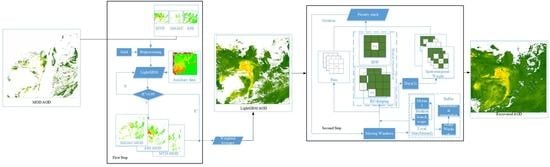
This paper proposes a two-step model (TWS) that combines the rich data volume of multisource data and the inherent spatial-temporal distribution relationships of aerosols to recover missing MOD AOD. First, we preprocess the multisource data and then use the TWS method to recover the MOD AOD. 1. For the multisource AOD data obtained at the same spatial location on the same day, some sources have pixel values, and some are missing. The existing data helps to recover some of the missing MOD AOD values from the other data sources, which is possible due to the complementarity of the multisource AOD data. The multisource AOD data is fitted and calculated using a machine learning method, and then the overlapping parts of the multisource AOD data are calculated by a weighted average to fill in some missing MOD AOD pixels. 2. In the moving window, the missing MOD AOD can be recovered through space or spatiotemporal relationships. First, we create a moving window. The corresponding calculation scenario is determined by the number and distribution of the AOD in the moving window and then combined with the buffer factor to perform the calculation. Finally, the recovered MOD AOD pixels are obtained by the priority settings of the overlapped pixels (priority stack). The steps of the specific method are shown in Figure 2.
3.1. Data Preprocessing
First, we create a 3-km spatial resolution grid in the UTM coordinate system. We rebuild the multisource data according to the grid position (including the AOD data set and auxiliary data). MAIAC AOD, AHI AOD, meteorological data, terrain data, and land data must be reconstructed because the spatial resolution is not 3 km. Specifically, MAIAC AOD, terrain data and NDVI must have their averages calculated in the 3-km grid. We summarize the population data within the 3-km grid (POP), and the RL data must have the total length of the roads in the grid calculated, which is assigned to the road length grid (RLG). All of the reproduced information must be resampled due to pixel position deviation.
3.2. First Step of TWS
GBM uses a gradient descent algorithm to adjust the regression tree of the weak learner’s addiction model, thereby reducing the loss of the objective function. LightGBM was developed by Microsoft and uses the GBM framework. LightGBM adds Gradient-based One-Side Sampling (GOSS) and Exclusive Feature Bundling (EFB). Compared with GBM, LightGBM can accelerate the calculation speed under the premise of ensuring accuracy, and has a higher calculation speed for large sample data [48,49]. In this study, MOD AOD was used as the dependent variable; MYD AOD, MAIAC AOD, AHI AOD and the other auxiliary data were used as independent variables. Three LightGBM models, i.e., MOD-MYD, MOD-MAIAC and MOD-AHI, were established. Then, the accuracy of the prediction model was verified by a 10-fold cross-validation method. The data for constructing the LightGBM model were randomly divided into ten groups. Cyclic verification was performed ten times, and one group was used for prediction verification, while the remaining nine were used as training samples. The decision coefficient (R2) was used as an index for model verification. Next, we used the trained model to predict the missing AOD of MOD AOD where MYD AOD, MAIAC AOD, and AHI AOD were not missing. After calculating the three LightGBM models, weighted average processing was performed on the overlapping pixels according to the LightGBM training result R2.
3.3. Second Step of TWS
AOD data has a strong spatial correlation (the R of adjacent MOD AOD is 0.9), but it also has a certain correlation in time (the R of adjacent time MOD AOD is 0.5). Therefore, when restoring MOD AOD information, we consider the spatial relationship of AOD and the spatiotemporal relationship. Moreover, the small moving window could reduce the uncertainty caused by AOD spatial heterogeneity.
3.3.1. Design of Moving Window Size and Selection of Interpolation Mode
Moving windows of different sizes will affect the number of valid MOD AOD pixels. However, a large moving window will cause serious spatial heterogeneity of MOD AOD, and will also affect the computing performance of the MOD AOD recovery. In this study, we set the size of the moving window to 3 × 3 pixels, 7 × 7 pixels, and a self-adaption window (from 3 pixels to 7 pixels) [34]. The self-adaption window is determined by the ratio of the number of valid AOD pixels to the total number of pixels. The formula is as follows:
where represents the size of the self-adaption window; is the number of valid AOD pixels in the window; and is the total number of pixels in the window.
Spatial interpolation and spatiotemporal interpolation methods have good adaptability to recover the AOD data, which performs a strong correlation in local space and is spatiotemporal. Regardless of whether it is spatial interpolation or spatiotemporal interpolation, the recovery results of the AOD data are greatly affected by the distribution and the number of valid AOD data points and the spatiotemporal distribution of the AOD data. Therefore, this study designed the following scenarios (taking a 3 × 3 window as an example), as shown in Figure 3: (1). Inverse Distance Weight interpolation (IDW) [50] is a spatial interpolation method. It was applied when the central MOD AOD was missing in the moving window. (2). We used region constraints kriging (RC kriging) which involves adding a constraints factor to the ordinary kriging method. It was applied when five or fewer pixels of MOD AOD were missing in the moving window. (3). We used spatiotemporal weight interpolation when the number of missing cells of Day 2 MOD AOD was greater than or equal to 5 and the number of valid AOD cells of Day 1 or Day 3 MOD AOD was greater than or equal to 5. (4). When there were too few MOD AOD pixels in the moving window for three consecutive days (Day 2 had no MOD AOD pixels and the number of valid MOD AOD cells for Days 1 and 3 were fewer than (5), we ignored this part of the calculation. The change in the window size changed the above rule (the ratio of the number of AOD pixels to the total number of moving window pixels). For example, when the window was 7 × 7, the five pixels in condition two increased to 27.
3.3.2. Buffer Factor
Because the moving window introduced only a small quantity of MOD AOD data, it caused the prediction value to deviate greatly between the spatial interpolation and spatiotemporal interpolation of MOD AOD. Therefore, a buffer factor was introduced to correct the deviation. Global Moran’s I (MoranI) [51] is a statistic for spatial autocorrelation; the larger the MoranI of AOD, the higher the similarity of the AOD data, which can provide more information for the recovery of AOD gaps. This approach is applied to calculate the spatial autocorrelation of MOD AOD in the region; the larger the value of MoranI, the higher the correlation of the MOD AOD data in the region. This study calculated MoranI in different areas and determined the maximum amount of MoranI in a local area. The corresponding local area was called the scope window (Figure 4). The mathematical expectation of the MOD AOD of the scope window served as a buffer factor for the spatial interpolation of the MOD AOD. Uncertainty in the numeric values of the MOD AOD pixels in the scope window was prone to occur, and the MOD AOD pixel values were not in a Gaussian distribution. The Spearman correlation coefficient was introduced as the time buffer factor of the MOD AOD. The mathematical expectation of the Spearman correlation coefficient for three consecutive days and the MOD AOD of the scope window were used as buffer factors for the spatiotemporal interpolation of the MOD AOD. The formula is as follows:
where MoranI represents the Global Moran’s I. Here, n represents the number of valid pixel AODs; and represent the AOD values of the two pixels, I and J; represents the average value of the AOD pixels; represents the spatial distance between the two pixels, I and J; represents the inverse distance weight; represents the window that corresponds to the maximum local MoranI, is a square; represents the number of pixels on one side of the square a ; represents iterative search for the ; represents obtaining ; represents the AOD value in the ; represents the AOD value in the on day ; represents the mathematical expectation of AOD in the (buffer factor); and represents the Spearman correlation coefficient between day and day .
3.3.3. Spatial Interpolation Method (IDW and RC Kriging)
Compared with other complicated physical models of AOD recovery, the spatial interpolation of AOD can quantify the spatial information of the AOD with known spatial positions, which can easily and effectively predict the missing AOD data over a small range. Moreover, the AOD spatial interpolation method does not require an excessive number of parameters. Among them, IDW and the spatial interpolation method are commonly used to predict the missing AOD. Additionally, based on the best linear unbiased prediction of ordinary kriging interpolation [52], we introduced the buffer factor for spatial interpolation when predicting the MOD AOD in a moving window, and established RC kriging. The buffer factor helps the RC kriging method to better adapt to the stability of mod AOD in the moving window [53]. The formula is as follows:
where and represent the AOD estimates produced by IDW interpolation and RC Kriging interpolation, represents the inverse distance weight, represents the MOD AOD value at points I and J, represents the Lagrange multiplier, represents the weight, and represent the covariance of and , and represents the mathematical expectation in the (buffer factor).
3.3.4. Spatiotemporal Weight Interpolation (STW)
Spatiotemporal interpolation can effectively consider both space and time MOD AOD relationships and overcome the shortcomings of MOD AOD space interpolation [54]. We quantify the time distance of one day of MOD AOD as 1 and combine the spatial distance between the MOD AOD pixels to determine the spatiotemporal distance. The spatiotemporal distance and the buffer factor are used to determine the spatiotemporal weight of MOD AOD spatiotemporal interpolation. We combine the spatiotemporal interpolation and spatiotemporal weights to generate spatiotemporal weight interpolation (STW). In this study, the time of STW used for MOD AOD was set to three days (including the predicted day, as well as the days before and after the predicted time), to avoid the excessive AOD data noise caused by a time span that is too long. The specific formula is as follows:
where represents the estimation of STW. T represents the time of day, t1 is the previous day, t2 is the day to be calculated, and t3 is the next day. represents the value of the valid AOD. is the mathematical expectation in within t days (buffer factor), represents the R between and . represents the time weight of k days (). is the number of pixels in the moving window, and represents the spatial distance between and .
3.3.5. Priority Setting of Overlapping Pixels
Because the spatial interpolation of MOD AOD and STW belong to the second step in TWS, TWS will have overlapping results of MOD AOD recovery with the movement of the window. Therefore, TWS should set the priority of the MOD AOD recovery results. The priority of the MOD AOD recovery result was set to IDW > RC Kriging > STW. If the MOD AOD recovery resulted in overlap, then the missing values of the MOD AOD were filled according to their priority. Furthermore, if the recovery results of the MOD AOD overlap in the same method, the average amount of the MOD AOD recovery results overlap should be calculated as the final result of the MOD AOD. For example, in the process of moving the window of TWS, RC kriging and STW were used in the two calculations before and after the predicted time, and the overlapping area of the MOD AOD recovery result should have used the RC kriging result. If RC kriging was used for both calculations during the window movement of the TWS, the overlapping area of the MOD AOD recovery results were calculated in the average value as the final MOD AOD recovery result.
3.3.6. Validation Methodology
A comparison between the MOD AOD recovery results and AERONET data can be used as the basis for the MOD AOD recovery accuracy [55]. The time resolutions of MOD AOD and AERONET were different. This research calculated the transit time of the satellite (Terra) (30 min before and after) and compared the average value of the AERONET data with the MOD AOD data of the location pixels for the AERONET site [37]. In addition, AERONET collected AOD data of multiple wavelengths, many of which were slightly different from the MOD AOD wavelength (550nm). Therefore, the AERONET AOD at 550 nm was interpolated using the Ångström exponent [7]. In addition, both the 551 nm and 560 nm AOD data were used in the AERONET data to evaluate the MOD AOD. The specific calculation formula is as follows:
where , , and represent the AOD at wavelengths , , , respectively. Here, represents the Ångström exponent.
The accuracy evaluation indexes include R and RMSE, where RMSE is as shown in Equation (6).
where and represent the AOD from MOD AOD and , respectively.
4. Results
4.1. LightGBM Training and Processing Results
We constructed and trained the three LightGBM models separately and combined them with 10-fold cross-validation; the sample size, R2, and independent input variables are listed in Table 2. Then, each of the three LightGBM models was used to predict the missing MOD AOD, and we superimposed the prediction results (where the overlap of the pixels is weighted according to R2); the results for 1 January 2018 are listed in Figure 5.
In Table 2, it can be seen that all of the auxiliary variables were involved in the training of the three groups of LightGBM models, and the R2 of the 10-fold cross-validation fitting effect exceeded 0.95. Additionally, in 1 January 2018, the MOD AOD gap was filled by MYD AOD, MAIAC AOD, and AHI AOD. Among them, AHI AOD contributed the largest quantity of AOD data. The AOD missing rate predicted by AHI AOD decreased from 90% to 56%. After calculating the weighted average of the overlapping parts, the AOD missing rate dropped to 47%.
4.2. Comparison between MOD AOD Recovered by Different Methods and AERONET
We compared the AOD data recovered by different methods with AERONET: 1. The original MOD AOD data and AERONET. 2. The first step of the TWS (LightGBM) was used to calculate the recovered AOD and AERONET comparison. 3. Using spatiotemporal kriging interpolation to interpolate the MOD AOD, we then compared the AOD results with AERONET data. 4. The TWS calculation results were compared with AERONET. To evaluate the effect of the TWS model more carefully, the accuracy of the comparison was divided into all of the AOD data parts (including the recovered part of the AOD and the original MOD AOD part) and a separate AOD recovery part (excluding the original MOD AOD data), as shown in Figure 6 and Figure 7.
As shown in Figure 6 and Figure 7, the number of matching points of MOD AOD and AERONET for reference are 263, the R is 0.83, and the Root Mean Square Error (RMSE) is 0.13. In the comparison of all of the AOD pixel values, LightGBM has the least number of matching points (n = 876), and although the number of matching points in the spatiotemporal kriging interpolation is the largest (1587), the quality according to the R and RMSE (0.59, 0.71) is not as good as that of LightGBM (0.85, 0.24), while TWS (R = 0.87, RMSE = 0.23) maintains value of the R with LightGBM and the reference and the quality of RMSE while also obtaining a larger number of matching points (1433). In the comparison of the AOD recovery part, we computed the results of the TWS recovery after removing MOD AOD (R = 0.87, RMSE = 0.26) and LightGBM (R = 0.88, RMSE = 0.25), and the R and the indicators of RMSE were removed from LightGBM MOD AOD (R = 0.86, RMSE = 0.26), which is consistent; the R is consistent with the reference (the difference in the RMSE index is related to the number and distribution of the reference samples). It can be seen from the results that TWS not only utilizes the information volume of the multisource AOD data, but also absorbs the advantages of AOD spatiotemporal information. In the case of increasing the number of matching points, the R can still maintain a high quality, which indicates that the TWS is reliable.
To further verify the effectiveness of TWS, we regridded the original MOD AOD by 5 × 5 AOD pixels size, and set the existing value in the grid center as a forced-missing AOD. Then, we used 3 × 3 grid TWS to regenerate the forced-missing MOD AOD. A validation between the regenerated MOD AOD and the original effective MOD AOD is shown in Figure 8.
As shown in Figure 8, the number of regenerated MOD AOD is 2352752. After restoring the missing AOD by 3 × 3 grid TWS, the validation process results in R = 0.98 and RMSE = 0.05 between the regenerated MOD AOD and the original effective MOD AOD. These results show that the 3 × 3 grid TWS also maintains good stability and accuracy in recovering a large number of missing MOD AOD pixels. This verifies the reliability of the TWS.
4.3. TWS Recovered the Performance with Different Moving Windows
The missing rate for MOD AOD was calculated by the ratio of the MOD AOD pixels and the total number of pixels in the study area, as shown in Figure 9. The MOD AOD missing rate was set to between 0 and 1. The recovery of MOD AOD requires higher accuracy and a lower MOD AOD missing rate to achieve its goal. Although the MOD AOD after the spatiotemporal kriging interpolation processing had no AOD data missing, the accuracy could not reach the application level. Therefore, the comparison of the MOD AOD missing rate was conducted in different windows of the TWS (3 × 3 window, adaptive window and 7 × 7 window). According to the statistics of the original MOD AOD data and the MOD AOD results recovered by TWS, the annual average missing rate of the original MOD AOD exceeded 0.8. After the first step of the TWS LightGBM calculation, the average annual missing rate of MOD AOD decreased from 0.8 to 0.4, and after 3 × 3 restoration of the window, the annual average missing rate of MOD AOD decreased from 0.4 to 0.1; additionally, the result calculated after the 7 × 7 window (0.06) showed the smallest annual average missing rate of MOD AOD.
Furthermore, in 2018, the standard deviation of the missing rate of MOD AOD after LightGBM alone was 0.131. However, the standard deviation of the MOD AOD missing rate of the TWS treatment was smaller than 0.08, which shows that LightGBM alone relies on only multisource AOD data. After processing by LightGBM alone, there is still a large quantity of missing AOD data. In contrast, a complete TWS combined with spatial and spatiotemporal information can reduce the missing rate of MOD AOD.
According to Table 3 and Figure 10, the missing rate of MOD AOD, R, and the calculation efficiency all change with changes in the size of the moving window. Among them, the 7 × 7 grid has the lowest R and the largest RMSE, 0.78 and 0.32, respectively. The adaptive R and RMSE are 0.79 and 0.3, respectively. The 7 × 7 grid and adaptive R decrease compared to the 3 × 3 window, while the RMSE increases. The adaptive network’s calculation time of the grid is the largest, i.e., 4.2 times that of the 3 × 3 grid, while the 7 × 7 grid is 2.7 times that of the 3 × 3 grid. The above data show that with the expansion in the window size, the result R from the recovery of the MOD AOD decreases, while the RMSE increases. A possible reason for this is that the spatial and temporal variability of the MOD AOD increases with the size of the moving window. Moreover, the change in the size of the moving window also significantly affects the amount of calculation.
4.4. Analysis of the Spatiotemporal Characteristics of MOD AOD Recovered by TWS
Combining the recovery results of the MOD AOD in the 3 × 3 window of the TWS and the spatiotemporal kriging interpolation results of the MOD AOD, the annual average results of the MOD AOD after recovery were calculated and compared with the annual average results of the original MOD AOD (Figure 11). The following can be found in Figure 11: (1). There were still some gaps in the annual average map of the original MOD AOD (the position of the red circle 1). Compared with Figure 1 (land use), the red circle is mainly brighter, bare land, which confirmed that the DT algorithm and the DB algorithm had poor AOD data inversion in relatively bright areas. The annual average result of the MOD AOD recovery in the 3 × 3 window of TWS and the annual average result of the MOD AOD spatiotemporal Kriging interpolation filled the gaps of the AOD data in the red circle 1. (2). The maximum value of the original annual average result of the MOD AOD is too large in Figure 11 (the maximum AOD value was 3). (3). The maximum value in the annual average result of MOD AOD in the 3 × 3 window of TWS decreased to 0.64 and the annual average result of the spatiotemporal kriging interpolation of MOD AOD decreased to 0.82. (4). The average value in the annual average results of the original MOD AOD, spatiotemporal kriging interpolation and TWS were 0.23, 0.34 and 0.27 respectively. The original MOD AOD data had a large number of missing AOD pixels (the missing rate in Figure 11a was 2%). There was a lack of sufficient AOD pixels to average the minimum and maximum values in the original MOD AOD, which ultimately led to the maximum value in the original MOD AOD annual average result being too large (the maximum AOD value was 3), and the average value in the original MOD AOD annual average result was low (the average AOD value was 0.23). (5). Comparing red circle 2, the annual average results of the original MOD AOD and the spatiotemporal Kriging interpolation of the MOD AOD are higher. The annual average results of the restoration of MOD AOD in the 3 × 3 window of TWS retained the original MOD AOD spatial characteristics of the annual average results and reduced the annual average of MOD AOD. Moreover, in the Pacific region, the annual average results of the restoration of the TWS 3 × 3 window MOD AOD were higher than the original annual average results of the original MOD AOD. In the original annual average results of the MOD AOD, the reason why the AOD data gap in red circle 1 was filled is that the 3 × 3 window of the TWS and the spatiotemporal kriging interpolation method filled the AOD data gap to a large extent. The reason for this was that the MOD AOD gap was filled, and the MOD AOD annual average result was more fully calculated. The maximum value of the original MOD AOD annual average result was reduced. In addition, due to the lack of accurate prediction of local features by the spatiotemporal kriging interpolation algorithm, the annual average result of the MOD AOD spatiotemporal kriging interpolation was higher than the average annual result of the restoration of the TWS 3 × 3 window MOD AOD.
We compared the results of the TWS 3 × 3 window MOD AOD recovery with the original MOD AOD data by a monthly average (Figure 12). In Figure 12, we marked the missing rate, average and maximum of the monthly average of the original MOD AOD and the monthly average of TWS AOD for each month. The monthly average maximum value of TWS AOD was smaller than the original monthly average maximum value of MOD AOD. The average range of the monthly average results of TWS AOD (0.17–0.24) was also smaller than the average monthly average results of the original MOD AOD (0.18–0.36). In addition, the TWS AOD monthly average result also accurately retained the high value area of the original MOD AOD monthly average result (in the yellow box).
On this basis, in the yellow box area in Figure 12 (112.7° E–125.2° E, 32.5° N–42.1° N), we calculated the monthly average and maximum AOD values of the original MOD AOD and TWS AOD in this area, as well as the monthly average AERONET AOD at the same place (Figure 13). In the yellow box area, the maximum of the monthly average original MOD AOD result was greater than 2. The maximum of the monthly average TWS AOD result was lower than the maximum of the monthly average original MOD AOD result. Moreover, the largest average value of the monthly average TWS AOD results was in June. Specifically, there was an upward trend from January to June and a downward trend from June to December. In addition, in the yellow box, there are seven AERONET ground stations. We calculated the monthly average of these stations. The monthly average trend of MOD AOD after TWS recovery was also consistent with the monthly average AERONET AOD trend. A similar trend was shown by Song et al. [56] for the North China Plain in 2018.
5. Discussion
5.1. Comparison of TWS and Other MOD AOD Recovery Models
The recovery of missing satellite AOD product data is of great significance to atmospheric pollution research. Recently, many methods have been used to study the recovery of missing data from satellite AOD products. This study selected the same approach to recover missing MOD AOD data and made a comparison in Table 4. The results of the various methods in Table 4 were compared with AERONET. Based on this comparison, the improvements in R compared to the MOD AOD and AERONET recovered by the proposed method and the R compared to the original MOD AOD and AERONET were not obvious (the R of the MOD AOD and AERONET recovered by the TWS recovery was the highest). In the comparison of the missing rate of MOD AOD, the missing rate of MOD AOD recovered by TWS was the lowest (0.1). Additionally, in the different methods in Table 4, the missing rate of the MOD AOD recovered by TWS had the largest decreased missing rate difference compared to the original MOD AOD (0.78). The improved difference (R) of the 3 × 3 window TWS method was not significantly different from other methods. However, the decreased missing rate difference (%) of the 3 × 3 window TWS method was significantly different from other methods. The main reasons are as follows: (1.) The 3 × 3 window TWS introduced multisource datasets (MYD AOD, MAIAC AOD, AHI AOD). With TWS, the first step is to use the spatial complement of AOD data sets with different algorithms and data collection times. The AOD missing rate dropped from 88% to 40%. In Figure 9, the decreased missing rate difference (%) is 48%. (2.) The second step of the 3 × 3 window TWS is to make reasonable use of the spatiotemporal relationship of AOD, under the optimization of moving window and buffer factor. The AOD missing rate decreased from 40% to 10% (the decreased missing rate difference (%) was 30%). Although the direct comparison of the decreased missing rate difference had certain limitations, it also showed stability and excellent performance for the TWS.
5.2. TWS Recovery MOD AOD Performance Discussion
The MOD AOD after TWS processing can obtain a higher improved R and lower AOD missing rate because it takes full advantage of the rich data volume of multisource data and the high local spatiotemporal autocorrelation of the AOD itself. A large amount of research has confirmed that multisource data can easily introduce data noise. However, based on the data statistics, we chose LightGBM to build a MOD AOD prediction model, which can make full use of the characteristics of different AOD data and reduce the data noise. From the comparison between LightGBM and AERONET, it can be seen that the LightGBM model does not introduce much data noise (all R = 0.85, R = 0.86 after removing MOD AOD).
Moreover, we developed MOD AOD recovery measures based on moving small windows by combining MOD AOD spatial data and spatiotemporal data when generating the statistics. The setting of the small window is used to ensure a high correlation of AOD in the small window. MOD AOD recovery measures set three MOD AOD recovery modes, and use the adaptive space and spatiotemporal buffering methods. Different calculation modes were set based on the temporal and spatial distribution of valid AOD information, to enable the calculation to be more reliable when recovering the AOD value. In this way, it can avoid the introduction of excessive data noise. The index was used to determine the local area of the autocorrelation, and the mathematical expectation and R were introduced to slow down the spatiotemporal difference; then, we determined the spatial and spatiotemporal buffer. Spatial and spatiotemporal buffering can more accurately improve the R of the moving small windows to recover the MOD AOD missing data. These settings all ensure the accuracy of the MOD AOD recovery and reduce the data loss rate of MOD AOD (R = 0.87 compared to MOD AOD and AERONET in the 3 × 3 window. The average daily loss rate of MOD AOD was 10%, whereas the adaptive window of the MOD AOD and AERONET comparison was R = 0.79, the average daily missing rate of MOD AOD was 8%, the window of the 7 × 7 window MOD AOD and AERONET comparison was R = 0.78, and the average daily missing rate of MOD AOD was 6%). In different applications, different window sizes can be chosen to meet different needs because the moving window size is variable. For example, to obtain a lower MOD AOD data loss rate, a larger moving window in TWS can be selected. The 7 × 7 window in the 2018 experiment can limit the average daily loss rate of MOD AOD to 6%. Therefore, moving the window size can adjust this advantage and make the TWS method more flexible. Moreover, if the missing MOD AOD data rate is not 0, the iterative approach to the TWS method can be used, which gradually reduces the missing MOD AOD data rate to 0. Of course, it is also possible to use spatial interpolation based on the results of MOD AOD processed by TWS to reduce the missing rate of MOD AOD to 0. Because TWS is based on sufficient data statistics on AOD data and uses AOD spatial autocorrelation, the TWS method can, in general, be applied to the missing data of AHI AOD, MAIAC AOD, MYD AOD and other remote sensing products with spatial correlation and time correlation. Finally, the MOD AOD recovered by TWS cannot be studied and used on a global scale because the AHI sensor is carried on a geosynchronous orbit satellite.
5.3. TWS Recovery MOD AOD
In the results of MOD AOD recovery in the study area in 2018 (Figure 11), we found that the areas with higher AOD were mainly concentrated in North China, the Central China Plain, the Yangtze River Delta and the Sichuan Basin; in northern Vietnam, the Japanese Islands and the Korean Peninsula, the AOD was lower (see Figure 12). Because of the dry weather conditions of the Red River Delta, in addition to local traffic and industrial pollution, there was a relatively obvious pollutant transmission process, and higher AOD distributions existed in southern China and northern Vietnam in March and April [57]. Moreover, there was also a higher monthly average value of AOD near the North China Plain and Shandong Peninsula in China which spread to the sea. Furthermore, in November, December and January, the pollutant diffusion capacity of North China, the Central China Plain and the Yangtze River Delta was more obvious during the influence of the winter monsoon [58,59]. Eventually, the mean monthly AOD of North China, the Central China Plain, the Yangtze River Delta and the East China Sea increased. Overall, the high AOD area did not cover the Korean Peninsula or the Japanese Islands. Although some of the pollutants might have reached the Korean Peninsula and the Japanese Archipelago region through the atmospheric transmission process, most of the pollutant transmission still stopped in the offshore area of China.
6. Conclusions
A high-precision, low AOD missing rate MOD AOD recovery result is of great help in measuring the spatial distribution of air pollutants, continuous monitoring, climate change and other related research. In this paper, the TWS model was constructed by multisource AOD data, LightGBM, spatial interpolation and STW, which were used for the large-scale recovery of data missing from MOD AOD. The results show that the TWS model can guarantee the accuracy of the recovered MOD AOD (R = 0.87). Moreover, compared with other methods, TWS greatly reduces the missing rate of the MOD AOD data (the missing rate of MOD AOD in the 3 × 3 window dropped from the original 88% to 10%). Moreover, after the missing information is added, the changes in the local AOD start to show more obvious high and low value details, for example, the AOD average, maximum and minimum of the original MOD AOD missing area in the AOD annual average map. TWS proves the spatial complementarity of multisource AOD data and the spatiotemporal relationship of the AOD data, which is very important when recovering the AOD data. In follow-up research, we will use other data sets to expand the applicability of the TWS method, for example, using GOES-16 ABI AOD data to restore AOD on the American continent. Moreover, we will use deep learning to recover areas in which the loss of AOD spatiotemporal information is severe, for example, in scenario 3 (Pass) in Figure 2, the moving window has missing AOD information for three consecutive days.
Author Contributions
Methodology, Y.C.; validation, Y.C.; formal analysis, Y.C.; writing—original draft preparation, Y.C.; writing—review and editing, Z.W., Y.R. and K.L. All authors have read and agreed to the published version of the manuscript.
Funding
This work was supported by the National Science Foundation of China (31670645, 31972951, 41801182, and 41807502), the National Social Science Fund (17ZDA058), the National Key Research Program of China (2016YFC0502704), Fujian Provincial Department of S&T Project (2018T3018), the Strategic Priority Research Program of the Chinese Academy of Sciences (XDA23020502), the Ningbo Municipal Department of Science and Technology (2019C10056), the Xiamen Municipal Department of Science and Technology (3502Z20130037 and 3502Z20142016), the Key Laboratory of Urban Environment and Health of CAS (KLUEH-C-201701), the Key Program of the Chinese Academy of Sciences (KFZDSW-324), and the Youth Innovation Promotion Association CAS (2014267). Open-end Fund (2020KX03).
Acknowledgments
We are grateful to the anonymous reviewers for their constructive suggestions. The authors would like to express our gratitude to the National Aeronautics and Space Administration (NASA) for providing the MODIS AOD, MAIAC, MERRA2, SRTM and NDVI products, gratitude to the Japan Meteorological Agency(JMA) and Center of Environmental Remote Sensing, Chiba University (CEReS) for providing the AHI AOD product, and the Principle Investigators for establishing and maintaining the AERONET sites.
Conflicts of Interest
The authors declare no conflict of interest
References
- Hallquist, M.; Wenger, J.C.; Baltensperger, U.; Rudich, Y.; Simpson, D.; Claeys, M.; Dommen, J.; Donahue, N.M.; George, C.; Goldstein, A.H.; et al. The formation, properties and impact of secondary organic aerosol: Current and emerging issues. Atmos. Chem. Phys. 2009, 9, 5155–5236. [Google Scholar] [CrossRef] [Green Version]
- Mahowald, N. Aerosol Indirect Effect on Biogeochemical Cycles and Climate. Science 2011, 334, 794–796. [Google Scholar] [CrossRef]
- Dubovik, O.; Holben, B.; Eck, T.F.; Smirnov, A.; Kaufman, Y.J.; King, M.D.; Tanré, D.; Slutsker, I. Variability of Absorption and Optical Properties of Key Aerosol Types Observed in Worldwide Locations. J. Atmos. Sci. 2002, 59, 590–608. [Google Scholar] [CrossRef]
- Ramanathan, V.; Crutzen, P.J.; Kiehl, J.T.; Rosenfeld, D. Aerosols, climate, and the hydrological cycle. Science 2001, 294, 2119–2124. [Google Scholar] [CrossRef] [PubMed] [Green Version]
- Adhikary, B.; Kulkarni, S.; Dallura, A.; Tang, Y.; Chai, T.; Leung, L.R.; Qian, Y.; Chung, C.E.; Ramanathan, V.; Carmichael, G.R. A regional scale chemical transport modeling of Asian aerosols with data assimilation of AOD observations using optimal interpolation technique. Atmos. Environ. 2008, 42, 8600–8615. [Google Scholar] [CrossRef]
- Xin, J.; Wang, Y.; Li, Z.; Wang, P.; Hao, W.; Nordgren, B.; Wang, S.; Liu, G.; Wang, L.; Wen, T.; et al. Aerosol optical depth (AOD) and Ångström exponent of aerosols observed by the Chinese Sun Hazemeter Network from August 2004 to September 2005. J. Geophys. Res. 2007, 112. [Google Scholar] [CrossRef]
- Holben, B.N.; Eck, T.F.; Slutsker, I.; Tanré, D.; Buis, J.P.; Setzer, A.; Vermote, E.; Reagan, J.A.; Kaufman, Y.J.; Nakajima, T.; et al. AERONET—A Federated Instrument Network and Data Archive for Aerosol Characterization. Remote Sens. Environ. 1998, 66, 1–16. [Google Scholar] [CrossRef]
- Giles, D.M.; Sinyuk, A.; Sorokin, M.G.; Schafer, J.S.; Smirnov, A.; Slutsker, I.; Eck, T.F.; Holben, B.N.; Lewis, J.R.; Campbell, J.R.; et al. Advancements in the Aerosol Robotic Network (AERONET) Version 3 database—Automated near-real-time quality control algorithm with improved cloud screening for Sun photometer aerosol optical depth (AOD) measurements. Atmos. Meas. Tech. 2019, 12, 169–209. [Google Scholar] [CrossRef] [Green Version]
- Zhao, C.; Liu, Z.; Wang, Q.; Ban, J.; Chen, N.X.; Li, T. High-resolution daily AOD estimated to full coverage using the random forest model approach in the Beijing-Tianjin-Hebei region. Atmos. Environ. 2019, 203, 70–78. [Google Scholar] [CrossRef]
- Remer, L.A.; Kaufman, Y.J.; Tanré, D.; Mattoo, S.; Chu, D.A.; Martins, J.V.; Li, R.R.; Ichoku, C.; Levy, R.C.; Kleidman, R.G.; et al. The MODIS Aerosol Algorithm, Products, and Validation. J. Atmos. Sci. 2005, 62, 947–973. [Google Scholar] [CrossRef] [Green Version]
- Levy, R.C.; Mattoo, S.; Munchak, L.A.; Remer, L.A.; Sayer, A.M.; Patadia, F.; Hsu, N.C. The Collection 6 MODIS aerosol products over land and ocean. Atmos. Meas. Tech. 2013, 6, 2989–3034. [Google Scholar] [CrossRef] [Green Version]
- Hsu, N.C.; Jeong, M.J.; Bettenhausen, C.; Sayer, A.M.; Hansell, R.; Seftor, C.S.; Huang, J.; Tsay, S.C. Enhanced Deep Blue aerosol retrieval algorithm: The second generation. J. Geophys. Res. Atmos. 2013, 118, 9296–9315. [Google Scholar] [CrossRef]
- Levy, R.C.; Remer, L.A.; Kleidman, R.G.; Mattoo, S.; Ichoku, C.; Kahn, R.; Eck, T.F. Global evaluation of the Collection 5 MODIS dark-target aerosol products over land. Atmos. Chem. Phys. 2010, 10, 10399–10420. [Google Scholar] [CrossRef] [Green Version]
- Hyer, E.J.; Reid, J.S.; Zhang, J. An over-land aerosol optical depth data set for data assimilation by filtering, correction, and aggregation of MODIS Collection 5 optical depth retrievals. Atmos. Meas. Tech. 2011, 4, 379–408. [Google Scholar] [CrossRef] [Green Version]
- Lyapustin, A.; Wang, Y.; Korkin, S.; Huang, D. MODIS Collection 6 MAIAC algorithm. Atmos. Meas. Tech. 2018, 11, 5741–5765. [Google Scholar] [CrossRef] [Green Version]
- Lyapustin, A.; Wang, Y.; Laszlo, I.; Kahn, R.; Korkin, S.; Remer, L.; Levy, R.; Reid, J.S. Multiangle implementation of atmospheric correction (MAIAC): 2. Aerosol algorithm. J. Geophys. Res. Atmos. 2011, 116. [Google Scholar] [CrossRef]
- Wei, J.; Huang, W.; Li, Z.; Xue, W.; Peng, Y.; Sun, L.; Cribb, M. Estimating 1-km-resolution PM2.5 concentrations across China using the space-time random forest approach. Remote Sens. Environ. 2019, 231, 111221. [Google Scholar] [CrossRef]
- Kikuchi, M.; Murakami, H.; Suzuki, K.; Nagao, T.M.; Higurashi, A. Improved Hourly Estimates of Aerosol Optical Thickness Using Spatiotemporal Variability Derived From Himawari-8 Geostationary Satellite. IEEE Trans. Geosci. Remote Sens. 2018, 56, 3442–3455. [Google Scholar] [CrossRef]
- Letu, H.; Nagao, T.M.; Nakajima, T.Y.; Riedi, J.; Ishimoto, H.; Baran, A.J.; Shang, H.; Sekiguchi, M.; Kikuchi, M. Ice Cloud Properties From Himawari-8/AHI Next-Generation Geostationary Satellite: Capability of the AHI to Monitor the DC Cloud Generation Process. IEEE Trans. Geosci. Remote Sens. 2019, 57, 3229–3239. [Google Scholar] [CrossRef]
- Zhan, Y.; Luo, Y.; Deng, X.; Chen, H.; Grieneisen, M.L.; Shen, X.; Zhu, L.; Zhang, M. Spatiotemporal prediction of continuous daily PM2.5 concentrations across China using a spatially explicit machine learning algorithm. Atmos. Environ. 2017, 155, 129–139. [Google Scholar] [CrossRef]
- Wei, J.; Li, Z.; Cribb, M.; Huang, W.; Xue, W.; Sun, L.; Guo, J.; Peng, Y.; Li, J.; Lyapustin, A.; et al. Improved 1 km resolution PM2.5 estimates across China using enhanced space–time extremely randomized trees. Atmos. Chem. Phys. 2020, 20, 3273–3289. [Google Scholar] [CrossRef] [Green Version]
- Ghotbi, S.; Sotoudeheian, S.; Arhami, M. Estimating urban ground-level PM10 using MODIS 3km AOD product and meteorological parameters from WRF model. Atmos. Environ. 2016, 141, 333–346. [Google Scholar] [CrossRef]
- Mhawish, A.; Banerjee, T.; Broday, D.M.; Misra, A.; Tripathi, S.N. Evaluation of MODIS Collection 6 aerosol retrieval algorithms over Indo-Gangetic Plain: Implications of aerosols types and mass loading. Remote Sens. Environ. 2017, 201, 297–313. [Google Scholar] [CrossRef]
- Zhang, R.; Di, B.; Luo, Y.; Deng, X.; Grieneisen, M.L.; Wang, Z.; Yao, G.; Zhan, Y. A nonparametric approach to filling gaps in satellite-retrieved aerosol optical depth for estimating ambient PM2.5 levels. Environ. Pollut. 2018, 243, 998–1007. [Google Scholar] [CrossRef] [PubMed]
- Lv, B.; Hu, Y.; Chang, H.H.; Russell, A.G.; Bai, Y. Improving the Accuracy of Daily PM2.5 Distributions Derived from the Fusion of Ground-Level Measurements with Aerosol Optical Depth Observations, a Case Study in North China. Environ. Sci. Technol. 2016, 50, 4752–4759. [Google Scholar] [CrossRef] [PubMed]
- Chi, Y.; Zuo, S.; Ren, Y.; Chen, K. The Spatiotemporal Pattern of the Aerosol Optical Depth (AOD) on the Canopies of Various Forest Types in the Exurban National Park: A Case in Ningbo City, Eastern China. Adv. Meteorol. 2019, 2019, 12. [Google Scholar] [CrossRef] [Green Version]
- Song, Z.; Fu, D.; Zhang, X.; Han, X.; Song, J.; Zhang, J.; Wang, J.; Xia, X. MODIS AOD sampling rate and its effect on PM2.5 estimation in North China. Atmos. Environ. 2019, 209, 14–22. [Google Scholar] [CrossRef]
- Cheng, L.; Li, L.; Chen, L.; Hu, S.; Yuan, L.; Liu, Y.; Cui, Y.; Zhang, T. Spatiotemporal Variability and Influencing Factors of Aerosol Optical Depth over the Pan Yangtze River Delta during the 2014–2017 Period. Int. J. Environ. Res. Public Health 2019, 16. [Google Scholar] [CrossRef] [Green Version]
- Alam, K.; Qureshi, S.; Blaschke, T. Monitoring spatio-temporal aerosol patterns over Pakistan based on MODIS, TOMS and MISR satellite data and a HYSPLIT model. Atmos. Environ. 2011, 45, 4641–4651. [Google Scholar] [CrossRef]
- Van Donkelaar, A.; Martin, R.V.; Levy, R.C.; da Silva, A.M.; Krzyzanowski, M.; Chubarova, N.E.; Semutnikova, E.; Cohen, A.J. Satellite-based estimates of ground-level fine particulate matter during extreme events: A case study of the Moscow fires in 2010. Atmos. Environ. 2011, 45, 6225–6232. [Google Scholar] [CrossRef]
- Huang, C.; Goward, S.N.; Masek, J.G.; Thomas, N.; Zhu, Z.; Vogelmann, J.E. An automated approach for reconstructing recent forest disturbance history using dense Landsat time series stacks. Remote Sens. Environ. 2010, 114, 183–198. [Google Scholar] [CrossRef]
- Pang, J.; Wang, X.; Shao, M.; Chen, W.; Chang, M. Aerosol optical depth assimilation for a modal aerosol model: Implementation and application in AOD forecasts over East Asia. Sci. Total Environ. 2020, 719, 137430. [Google Scholar] [CrossRef] [PubMed]
- Zhang, T.; Zeng, C.; Gong, W.; Wang, L.; Sun, K.; Shen, H.; Zhu, Z.; Zhu, Z. Improving Spatial Coverage for Aqua MODIS AOD using NDVI-Based Multi-Temporal Regression Analysis. Remote Sens. 2017, 9. [Google Scholar] [CrossRef] [Green Version]
- Wang, Y.; Yuan, Q.; Li, T.; Shen, H.; Zheng, L.; Zhang, L. Large-scale MODIS AOD products recovery: Spatial-temporal hybrid fusion considering aerosol variation mitigation. ISPRS J. Photogramm. 2019, 157, 1–12. [Google Scholar] [CrossRef]
- Singh, M.K.; Venkatachalam, P.; Gautam, R. Geostatistical Methods for Filling Gaps in Level-3 Monthly-Mean Aerosol Optical Depth Data from Multi-Angle Imaging SpectroRadiometer. Aerosol Air Qual. Res. 2017, 17, 1963–1974. [Google Scholar] [CrossRef] [Green Version]
- Yang, J.; Hu, M. Filling the missing data gaps of daily MODIS AOD using spatiotemporal interpolation. Sci. Total Environ. 2018, 633, 677–683. [Google Scholar] [CrossRef] [PubMed]
- Tang, Q.; Bo, Y.; Zhu, Y. Spatiotemporal fusion of multiple-satellite aerosol optical depth (AOD) products using Bayesian maximum entropy method. J. Geophys. Res. Atmos. 2016, 121, 4034–4048. [Google Scholar] [CrossRef] [Green Version]
- Nam, J.; Kim, S.-W.; Park, R.J.; Park, J.-S.; Park, S.S. Changes in column aerosol optical depth and ground-level particulate matter concentration over East Asia. Air Qual. Atmos. Health 2018, 11, 49–60. [Google Scholar] [CrossRef]
- Xiao, Q.; Zhang, H.; Choi, M.; Li, S.; Kondragunta, S.; Kim, J.; Holben, B.; Levy, R.C.; Liu, Y. Evaluation of VIIRS, GOCI, and MODIS Collection 6 AOD retrievals against ground sunphotometer observations over East Asia. Atmos. Chem. Phys. 2016, 16, 1255–1269. [Google Scholar] [CrossRef] [Green Version]
- Hsu, N.C.; Si-Chee, T.; King, M.D.; Herman, J.R. Aerosol properties over bright-reflecting source regions. IEEE Trans. Geosci. Remote. 2004, 42, 557–569. [Google Scholar] [CrossRef]
- Xia, X.; Min, J.; Wang, Y.; Shen, F.; Yang, C.; Sun, Z. Assimilating Himawari-8 AHI aerosol observations with a rapid-update data assimilation system. Atmos. Environ. 2019, 215, 116866. [Google Scholar] [CrossRef]
- Jiang, J.H.; Su, H.; Zhai, C.; Wu, L.; Minschwaner, K.; Molod, A.M.; Tompkins, A.M. An assessment of upper troposphere and lower stratosphere water vapor in MERRA, MERRA2, and ECMWF reanalyses using Aura MLS observations. J. Geophys. Res. Atmos. 2015, 120, 468–485. [Google Scholar] [CrossRef] [Green Version]
- Tobin, K.W.; Bhaduri, B.L.; Bright, E.A.; Cheriyadat, A.; Karnowski, T.P.; Palathingal, P.J.; Potok, T.E.; Price, J.R. Automated Feature Generation in Large-Scale Geospatial Libraries for Content-Based Indexing. Photogramm. Eng. Remote Sens. 2006, 72, 531–540. [Google Scholar] [CrossRef]
- Fensholt, R.; Rasmussen, K.; Nielsen, T.T.; Mbow, C. Evaluation of earth observation based long term vegetation trends—Intercomparing NDVI time series trend analysis consistency of Sahel from AVHRR GIMMS, Terra MODIS and SPOT VGT data. Remote Sens. Environ. 2009, 113, 1886–1898. [Google Scholar] [CrossRef]
- Wei, J.; Li, Z.; Sun, L.; Peng, Y.; Zhang, Z.; Li, Z.; Su, T.; Feng, L.; Cai, Z.; Wu, H. Evaluation and uncertainty estimate of next-generation geostationary meteorological Himawari-8/AHI aerosol products. Sci. Total Environ. 2019, 692, 879–891. [Google Scholar] [CrossRef]
- Kaufman, Y.J.; Tanré, D.; Boucher, O. A satellite view of aerosols in the climate system. Nature 2002, 419, 215–223. [Google Scholar] [CrossRef]
- Miller, R.L.; Tegen, I. Climate Response to Soil Dust Aerosols. J. Climate 1998, 11, 3247–3267. [Google Scholar] [CrossRef]
- Zhang, J.; Mucs, D.; Norinder, U.; Svensson, F. LightGBM: An Effective and Scalable Algorithm for Prediction of Chemical Toxicity–Application to the Tox21 and Mutagenicity Data Sets. J. Chem. Inf. Model 2019, 59, 4150–4158. [Google Scholar] [CrossRef]
- Ke, G.; Meng, Q.; Finley, T.; Wang, T.; Chen, W.; Ma, W.; Ye, Q.; Liu, T.-Y. LightGBM: A highly efficient gradient boosting decision tree. In Proceedings of the 31st International Conference on Neural Information Processing Systems, Long Beach, CA, USA, 4–9 December 2017; pp. 3149–3157. [Google Scholar]
- Lu, G.Y.; Wong, D.W. An adaptive inverse-distance weighting spatial interpolation technique. Comput. Geosci. UK 2008, 34, 1044–1055. [Google Scholar] [CrossRef]
- Requia, W.J.; Dalumpines, R.; Adams, M.D.; Arain, A.; Ferguson, M.; Koutrakis, P. Modeling spatial patterns of link-based PM2.5 emissions and subsequent human exposure in a large canadian metropolitan area. Atmos. Environ. 2017, 158, 172–180. [Google Scholar] [CrossRef]
- Giraldo, R.; Delicado, P.; Mateu, J. Ordinary kriging for function-valued spatial data. Environ. Ecol. Stat. 2011, 18, 411–426. [Google Scholar] [CrossRef] [Green Version]
- Zhang, L.W.; Zhu, P.; Liew, K.M. Thermal buckling of functionally graded plates using a local Kriging meshless method. Compos. Struct. 2014, 108, 472–492. [Google Scholar] [CrossRef]
- Addesso, P.; Longo, M.; Montone, R.; Restaino, R.; Vivone, G. Interpolation and combination rules for the temporal and spatial enhancement of SEVIRI and MODIS thermal image sequences. Int. J. Remote. Sens. 2017, 38, 1889–1911. [Google Scholar] [CrossRef] [Green Version]
- Fu, D.; Xia, X.; Wang, J.; Zhang, X.; Li, X.; Liu, J. Synergy of AERONET and MODIS AOD products in the estimation of PM2.5 concentrations in Beijing. Sci. Rep. UK 2018, 8, 10174. [Google Scholar] [CrossRef] [PubMed] [Green Version]
- Song, Z.; Fu, D.; Zhang, X.; Wu, Y.; Xia, X.; He, J.; Han, X.; Zhang, R.; Che, H. Diurnal and seasonal variability of PM2.5 and AOD in North China plain: Comparison of MERRA-2 products and ground measurements. Atmos. Environ. 2018, 191, 70–78. [Google Scholar] [CrossRef]
- Trinh, T.T.; Trinh, T.T.; Le, T.T.; Nguyen, T.D.H.; Tu, B.M. Temperature inversion and air pollution relationship, and its effects on human health in Hanoi City, Vietnam. Environ. Geochem. Health 2019, 41, 929–937. [Google Scholar] [CrossRef]
- Kim, S.-W.; Yoon, S.-C.; Kim, J.; Kim, S.-Y. Seasonal and monthly variations of columnar aerosol optical properties over east Asia determined from multi-year MODIS, LIDAR, and AERONET Sun/sky radiometer measurements. Atmos. Environ. 2007, 41, 1634–1651. [Google Scholar] [CrossRef]
- Ju, Y. Tracking the PM2.5 inventories embodied in the trade among China, Japan and Korea. J. Econ. Issues 2017, 6, 27. [Google Scholar] [CrossRef] [Green Version]
Figure 1.
Distribution of the AERONET sites considered in this paper.

Figure 2.
Flowchart of the proposed TWS model. The recovered AOD represents the final result.

Figure 3.
Three scenarios of the second step TWS. Here, n represents the number of missing AOD pixels in the moving window, and Days 1, 2, and 3 represent three consecutive days (where Days 1 and 3 are disordered). 1—Spatial represents spatial interpolation, including IDW and RC kriging. 2—Spatiotemporal-weight represents spatiotemporal weighted interpolation and lists two examples. 3—Pass indicates that this scenario ignores and does not calculate the AOD in the moving window.

Figure 4.
Buffer factor calculation flowchart.

Figure 5.
MOD AOD is recovered from multisource AOD data and auxiliary data after fitting by LightGBM (2018.1.1). Here, (a) shows the original MOD AOD data (90% missing AOD); (b) shows the MOD AOD (56% missing AOD) after AHI AOD, and the auxiliary data were recovered by LightGBM; (c) shows the MOD AOD after combining MYD AOD and the auxiliary data after LightGBM recovery (84% missing AOD); (d) shows the MOD AOD (66% missing AOD) after combining MAIAC AOD and the auxiliary data after LightGBM recovery; (e) shows the result of calculating the weighted average of the overlapping parts of (b), (c) and (d) (47% missing AOD). The legend is the value range of the MOD AOD.

Figure 6.
Comparison of MOD AOD recovered by different methods (including the recovered MOD AOD and original MOD AOD) and AERONET. (a) Comparison of the original MOD AOD and AERONET. (b) Comparison of the MOD AOD recovered by LightGBM and AERONET. (c) Comparison of the MOD AOD recovered by spatiotemporal kriging interpolation and AERONET. (d) Comparison of the MOD AOD recovered by TWS with AERONET. The solid red line represents the regression line; the solid black line is the 1:1 line. The color bars represent the density of the points.

Figure 7.
Comparison of MOD AOD and AERONET recovered by different methods. (a). Comparison of the recovered MOD AOD of LightGBM (excluding the original MOD AOD part) and AERONET. (b). Comparison of the MOD AOD recovered by TWS (excluding the original MOD AOD part) and AERONET. (c). Comparison of the MOD AOD recovered by TWS (excluding the original MOD AOD and LightGBM recovered MOD AOD) and AERONET. The solid red line represents the regression line; the solid black line is the 1:1 line. The colored bars represent the density of the points.

Figure 8.
Comparison of the regenerated MOD AOD by 3 × 3 TWS and the original MOD AOD. The solid red line represents the regression line; the solid black line is the 1:1 line. The colored bars represent the density of the points.
Figure 8.
Comparison of the regenerated MOD AOD by 3 × 3 TWS and the original MOD AOD. The solid red line represents the regression line; the solid black line is the 1:1 line. The colored bars represent the density of the points.

Figure 9.
Time series plot of daily AOD coverage over study areas in 2018 for MOD, LightGBM, 3 × 3, self-adaption and 7 × 7. MOD represents the original MOD AOD, LightGBM represents LightGBM recovered MOD AOD, 3 × 3 represents the 3 × 3 grid moving window TWS recovered MOD AOD, self-adaption represents the self-adaption moving window TWS recovered MOD AOD, and 7 × 7 represents the 7 × 7 moving window TWS recovered MOD AOD. The numbers in parentheses represent the average and standard deviation of the empty AOD coverage.

Figure 10.
Comparison of TWS recovered MOD AOD (including the recovered MOD AOD and original MOD AOD) and AERONET in different moving windows. a. Comparison of the 7 × 7 moving window TWS recovery MOD AOD and AERONET. b Comparison of the self-adaption moving window TWS recovery MOD AOD and AERONET. The solid red line represents the regression line; the solid black line is the 1:1 line. The colored bars represent the density of points.

Figure 11.
The average annual MOD AOD distribution in 2018. (a). Annual average of the original MOD AOD (2% missing). (b). The MOD AOD average of the spatiotemporal kriging interpolation recovery (missing 0). (c). The 3 × 3 moving window TWS recovered the MOD AOD annual average (missing 0). The red fonts Ave and Max represent the average and maximum values of the AOD annual average graph, respectively. The white part represents nodata. The color bar represents the MOD AOD value.

Figure 12.
Monthly average of the original MOD AOD and 3 × 3 moving window TWS recovered MOD AOD (each month includes the missing rate of MOD AOD). The red fonts Ave and Max represent the average and maximum values of the AOD monthly average graph, respectively. The white part represents no data. The yellow box area represents the sampling area in Figure 13. The color bar represents the MOD AOD value.

Figure 13.
The broken line represents the monthly average original MOD AOD and the monthly average MOD AOD restored by TWS, respectively, and the dotted line represents the monthly average AERONET AOD, with the ordinate on the left. The histogram represents the maximum value (monthly) of the original MOD AOD and the MOD AOD recovered by TWS, respectively, with the ordinate on the right. The above data is from the yellow box area of Figure 12.


Table 1.
MOD AOD correlation (spatial correlation, temporal correlation, and correlation of different AOD data sources).
Table 1.
MOD AOD correlation (spatial correlation, temporal correlation, and correlation of different AOD data sources).
| R | |||
|---|---|---|---|
| MOD AOD spatial correlation | R = 0.92 (n = 13,489,645) | ||
| MOD AOD time correlation | R = 0.57 (n = 15,895,438) | ||
| Time correlation of multisource AOD data (compared with MOD AOD) | MYD | MAIAC | AHI |
| R = 0.56 (n = 7,746,528) | R = 0.77 (n = 10,125,868) | R = 0.56 (n = 15,256,795) | |
Note: n represents the number of observations.
Table 2.
LightGBM results and other variables.
| Group | Auxiliary Independent Variables | n | R2 |
|---|---|---|---|
| MOD AOD-MYD AOD | TLML, SPEED, ZM, QSH, PBLH, NDVI, POP, RLG, DOY, Slope, Aspect and Elevation | 2,112,108 | 0.964 |
| MOD AOD-MAIAC AOD | 4,226,536 | 0.975 | |
| MOD AOD-AHI AOD | 5,784,070 | 0.956 |
Table 3.
Performance comparison of 3 different moving windows.
| Windows | R (Total) | Incompleteness (%) | Time Ratio (%) |
|---|---|---|---|
| 3 × 3 grid | 0.85 | 10 | 100 |
| 7 × 7 grid | 0.78 | 6 | 225 |
| Self-adaption grid | 0.79 | 8 | 423 |
Table 4.
Comparison of the MOD AOD data recovery methods.
| Method | Original Missing Rate (%) | Improved Missing Rate (%) | Decreased Missing Rate Difference (%) | Original R | Improved R | Improved Difference (R) | Source |
|---|---|---|---|---|---|---|---|
| ST-AVM | 80 | 60 | 20 | 0.89 | 0.87 | −0.02 | [34] |
| NWRL | ~70 | ~60 | ~10 | 0.77 | 0.78 | +0.01 | [33] |
| * | 89 | 75 | 14 | 0.93 | 0.91 | −0.02 | [28] |
| TWS (3 × 3) | 88 | 10 | 78 | 0.83 | 0.87 | +0.04 | Our paper |
Note: ~ indicates a lack of accurate data in the cited article. * indicates a lack of method name in the cited article.
Publisher’s Note: MDPI stays neutral with regard to jurisdictional claims in published maps and institutional affiliations. |
© 2020 by the authors. Licensee MDPI, Basel, Switzerland. This article is an open access article distributed under the terms and conditions of the Creative Commons Attribution (CC BY) license (http://creativecommons.org/licenses/by/4.0/).
Share and Cite
MDPI and ACS Style
Chi, Y.; Wu, Z.; Liao, K.; Ren, Y. Handling Missing Data in Large-Scale MODIS AOD Products Using a Two-Step Model. Remote Sens. 2020, 12, 3786. https://doi.org/10.3390/rs12223786
AMA Style
Chi Y, Wu Z, Liao K, Ren Y. Handling Missing Data in Large-Scale MODIS AOD Products Using a Two-Step Model. Remote Sensing. 2020; 12(22):3786. https://doi.org/10.3390/rs12223786
Chicago/Turabian StyleChi, Yufeng, Zhifeng Wu, Kuo Liao, and Yin Ren. 2020. "Handling Missing Data in Large-Scale MODIS AOD Products Using a Two-Step Model" Remote Sensing 12, no. 22: 3786. https://doi.org/10.3390/rs12223786
Note that from the first issue of 2016, this journal uses article numbers instead of page numbers. See further details here.