Evaluation of Remote Sensing and Reanalysis Snow Depth Datasets over the Northern Hemisphere during 1980–2016


1
National Forestry and Grassland Administration Key Laboratory of Forest Resources Conservation and Ecological Safety on the Upper Reaches of the Yangtze River, Sichuan Province Key Laboratory of Ecological Forestry Engineering on the Upper Reaches of the Yangtze River, College of Forestry, Sichuan Agricultural University, Chengdu 611130, China
2
Heihe Remote Sensing Experimental Research Station, Key Laboratory of Remote Sensing of Gansu Province, Northwest Institute of Eco-Environment and Resources, Chinese Academy of Sciences, Lanzhou 730000, China
3
Jiangsu Center of Collaborative Innovation in Geographical Information Resource Development and Application, Nanjing 210023, China
*
Author to whom correspondence should be addressed.
Remote Sens. 2020, 12(19), 3253; https://doi.org/10.3390/rs12193253
Submission received: 24 August 2020
/
Revised: 25 September 2020
/
Accepted: 28 September 2020
/
Published: 7 October 2020
(This article belongs to the Special Issue Fusion of High-Level Remote Sensing Products)
Abstract
:Snow cover is a key parameter of the climate system and its significant seasonal and annual variability have significant impacts on the surface energy balance and global water circulation. However, current snow depth datasets show large inconsistencies and uncertainties, which limit their applications in climate change projections and hydrological processes simulations. In this study, a comprehensive assessment of five hemispheric snow depth datasets was carried out against ground observations from 43,391 stations. The five snow depth datasets included three remote sensing datasets, i.e., Advanced Microwave Scanning Radiometer for the Earth Observing System (AMSR-E), Advanced Microwave Scanning Radiometer-2 (AMSR2), Global Snow Monitoring for Climate Research (GlobSnow), and two reanalysis datasets, i.e., ERA-Interim and the Modern-Era Retrospective Analysis for Research and Applications, version 2 (MERRA-2). Assessment results imply that the spatial distribution of GlobSnow and ERA-Interim exhibit overall better agreements with ground observations than other datasets. GlobSnow and ERA-Interim exhibit less uncertainty during the snow accumulation and ablation periods, respectively. In plain and forested regions, GlobSnow, ERA-Interim and MERRA-2 show better performances, while in mountain and forested mountain areas, GlobSnow exhibits the best performance. AMSR-E and AMSR2 agree better with ground observations in shallow snow condition (0–10 cm), while MERRA-2 shows more satisfying performance when snow depth exceeds 50 cm. These systematic and integrated understanding of the five representative snow depth datasets provides information on data selection and data refinement, as well as data fusion, which is our next work of interest.
1. Introduction
Snow cover is the most widely distributed and most dynamic component of the cryosphere, and its significant seasonal and annual variability have notable influences on the global water circulation and surface energy balance [1,2,3]. Snow melt supplies water for approximately one sixth of the world’s population, and is a valuable water resource in arid and semi-arid regions [4,5,6]. Snow cover is not only a sensitive indicator that responds to the climate system, but is also an important feedback variable that amplifies global warming [7,8,9]. Therefore, under the goal of constraining the global mean temperature rise to 1.5 °C by 2100 according to the Paris Agreement [10], more attention should be paid to studies on snow cover change and its influence on global warming [11,12].
Reliable snow cover and snow depth datasets are, therefore, essential for global climate monitoring and water circulation research [13,14,15,16]. However, the data accuracy of snow depth is less satisfactory than that of snow cover extent. According to the fifth assessment report (AR5) of the Intergovernmental Panel on Climate Change (IPCC), there is very high confidence that the spring snow cover extent over the Northern Hemisphere has decreased since the mid-20th century, but only a lower data accuracy of snow depth than that of snow cover extent was noted [17]. In the Special Report “The Ocean and Cryosphere in a Changing Climate” of IPCC AR6, change in snow depth over the Northern Hemisphere during the 20th century had still not been clarified [18].
Ground observations represent the most direct and reliable snow depth data source, and mainly include observations from meteorological stations, snow surveys, and hydrological stations [19]. However, they are generally not used directly to monitor snow depth at hemispheric scales, in consideration of the inadequate amount of measurements and the uneven availability that is distributed very rarely in remote regions, mountains, and high elevation areas [20,21]. Snow water equivalent (SWE) is also an important snow cover parameter, it directly measures the total water amount of snow and is a function of snow depth and snow density. Nevertheless, when compared with snow depth measurements, field SWE and snow density measurements are more time consuming, and need more specialized instrumentations both in the fields and at the stations [22]. Thus, SWE or snow density measurements are much fewer than those of snow depth worldwide [23]. As a consequence, in this study we selected snow depth, rather than SWE, as the assessment metric.
Apart from ground observations, the available hemispheric/global snow depth datasets are mainly derived from microwave remote sensing, model simulations and reanalysis. The snow depth from microwave remote sensing datasets is usually retrieved based on its linear relationship with the brightness temperature gradient at different microwave frequencies (e.g., at 18 GHz and 36.5 GHz) [24]. Representative microwave remote sensing snow depth datasets include the Advanced Microwave Scanning Radiometer for the Earth Observing System (AMSR-E) snow depth dataset, its follow-on, the Advanced Microwave Scanning Radiometer-2 (AMSR2) snow depth dataset, the Global Snow Monitoring for Climate Research (GlobSnow) SWE dataset, etc. Snow models are a series of formulations constructed based on the physical properties of snow cover and related parameters, through which they can simulate spatial-temporal continuous snow evolution processes with certain forcing data [25,26]. Typical snow models include snowpack models (e.g., Crocus) and snow modules in land surface models (e.g., Global Land Data Assimilation System (GLDAS)). Atmospheric reanalyses generally consist of global atmospheric data assimilation systems that assimilate historical data spanning over an extended period, providing various land surface and atmospheric parameters in near real time [27,28]. Representative reanalyses include the ERA-Interim and Modern-Era Retrospective Analysis for Research and Applications, version-2 (MERRA-2), as well as their series datasets.
Snow depth datasets are characterized by significant differences regardless of data sources [29,30,31]. AMSR-E and GlobSnow show different spatial patterns and values, which is particularly obvious in Siberia [32]. Peak SWE from 18 global atmospheric general circulation models (AGCMs) that participate in the second phase of the Atmospheric Model Intercomparison Project (AMIP-2) varies for more than three times over North America [33]. The annual average peak SWE from remote sensing datasets, reanalyses, and model outputs over the Northern Hemisphere for the period 1981–2010 varies by as much as 50% [34].
Traditional remote sensing datasets, e.g., AMSR-E and AMSR2, show general limitations in deep snowpacks [35,36]. Model and reanalysis derived snow depth datasets show large uncertainties in forests, mountain areas, and during the snow ablation period [37,38,39], for which microwave remote sensing snow depth datasets also perform poorly [40,41,42]. General uncertainties of snow depth datasets were characterized through these evaluations, but more details are needed to fully understand the advantages and limitations of these datasets.
Several studies suggest that GlobSnow generally performed better against AMSR-E and AMSR2 in forested areas, such as in Finland and Russia [43,44], Northeast China [40], Eastern Canada [45], etc. However, the results from Eastern Canada indicate that the uncertainty of AMSR-E and AMSR2 data was significantly greater than that of GlobSnow only when SWE is larger than 150 mm and when forest cover is larger than 70%. Therefore, the performance of AMSR-E and AMSR2 in relatively shallow snow and non-forested conditions has probably been neglected and thereby needs further assessment.
Four reanalysis snow depth datasets (ERA-Interim, ERA-Interim/Land, MERRA, MERRA-Land), two models (GLDAS1, GLDAS2), and two observation-based snow depth datasets (GlobSnow, Canadian Meteorological center daily snow depth analysis (CMC)) were evaluated over mountainous areas in British Columbia, Canada, and the results suggest that MERRA performs generally better than GlobSnow and ERA-Interim [46]. A similar evaluation study that was conducted over the Saint-Maurice river basin region of Southern Québec, however, found that ERA-Interim and GlobSnow perform better than MERRA and MERRA-2 [47]. Regional evaluations provide detailed information on different datasets, but different study areas, reference data and different study periods may all lead to contradictory results, thus hemispheric evaluations of longtime series are essential to comprehensively understand these datasets.
Recently, several remote sensing, model outputs and reanalysis snow depth datasets, including AMSR-E, GlobSnow, Crocus, ERA-land, GLDAS-2, and MERRA were compared to snow survey data from Canadian, Finnish, and Russian sources as reference data. As a result, notable differences and larger uncertainties were found in AMSR-E when compared with other datasets, while Crocus and MERRA showed quite a good performance [48]. This work provides valuable insight into the relative performance of multiple datasets, but the study area only covers part of high latitudes of the Northern Hemisphere, and the evaluation period only lasts for winter months of 2002–2010, which is insufficient compared to the almost 40 years duration of reanalyses and model outputs.
Interestingly, quite a few evaluation studies noted that there is no universally best dataset, and that a combined dataset, or simply the ensemble mean would perform better than the individual datasets [33,39,49,50]. Therefore, combining multiple sources of datasets is a promising approach for obtaining more reliable snow depth estimates, and it will be our next work. However, data fusion should build on a solid and comprehensive recognition of the strengths and limitations of multiple snow depth datasets, which is apparently inadequate at present. To fill this gap, evaluations containing more types of datasets, broader study area, longer evaluation duration, and more systematic evaluation schemes are needed.
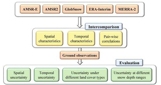
To improve the understanding of the uncertainties of snow depth datasets and prepare for future data fusion, this study provides a comprehensive evaluation on multiple hemispheric snow depth datasets. By examining their spatial and temporal characteristics, performances under different land cover types and at different snow depth ranges, the assessment focuses on investigating the uncertainties of individual dataset, differences of uncertainties among datasets, as well as the reasons behind. The paper is arranged as follows. Data and evaluation index are described in Section 2. The results were introduced in Section 3 with two subsections, the intercomparison about the spatial and temporal consistencies among different datasets, and assessment against ground observations. Discussion and conclusion follow by in Section 4 and Section 5, respectively.
2. Data and Methods
In this Section, we introduce five hemispheric snow depth datasets being evaluated, four reference data and two ancillary data, as well as the evaluation scheme. Specifically, brief information and basic algorithms of the five snow depth datasets, including AMSR-E, AMSR2, GlobSnow, ERA-Interim, and MERRA-2, are described in Section 2.1. Ground reference data, including meteorological station data from China and Russia, snow survey data from Russia and the Global Historical Climatology Network (GHCN)-Daily dataset are described in Section 2.2. A digital elevation model (DEM) data and a land cover data which were imported to extract mountain and forested areas are introduced in Section 2.3. The evaluation scheme is described in Section 2.4.
2.1. Hemispheric Snow Depth Datasets
2.1.1. AMSR-E and AMSR2 Daily Snow Depth Datasets
Advanced Microwave Scanning Radiometer for the Earth Observing System (AMSR-E) is a passive microwave sensor onboard the Aqua satellite, it was launched in 2002 and stopped working in 2011. Then, the Advanced Microwave Scanning Radiometer-2 (AMSR2), a successor of AMSR-E, was launched in 2012 onboard the Global Change Observation Mission 1st–Water (GCOM-W1) satellite [51]. Global SWE and snow depth datasets of AMSR-E and AMSR2 are provided by the National Aeronautics and Space Administration (NASA), and the Japanese Aerospace Exploration Agency (JAXA), respectively. In this study, we used the AMSR-E and AMSR2 snow depth datasets of from JAXA.
AMSR-E and AMSR2 daily snow depth datasets from JAXA use the retrieval algorithm from Kelly [52]. Before the snow depth retrieval, the “snow-free” area was identified and masked out by a hemispheric snow cover dataset [53] and MODQ11, a land cover dataset from Moderate Resolution Imaging Spectroradiometer (MODIS) [54]. Then, if the snow was considered shallow snow by the brightness temperature threshold detection, snow depth was set constant to 5 cm. For moderate or deep snow, an improved Chang algorithm that takes the forest cover fraction into consideration was implemented, and different coefficients were applied [55]. The most significant improvements of AMSR2 against AMSR-E are the smaller footprint and the optimization of the calibration system [56]. Although there is no temporal overlap between the two datasets, they are both cross calibrated against the Special Sensor Microwave Imager/Sounder (SSMI/S) to balance systematic errors.
AMSR-E and AMSR2 daily snow depth data were extracted for the periods 2003–2011 and 2013–2016, respectively (https://suzaku.eorc.jaxa.jp/). Note that in our study, a snow year is defined from September 1st of the previous year to August 31st of the current year. A spatial resolution of 0.25° × 0.25° was adopted for both AMSR-E and AMSR2 datasets, although AMSR2 also offers a finer spatial resolution of 0.10° × 0.10°. In addition, as daily detections of AMSR-E and AMSR2 do not fully cover the extent of the Northern Hemisphere, stripe gaps southward of 55 °N can be found in the daily images. Specifications of AMSR-E and AMSR2 (as well as other datasets introduced below) are displayed in Table 1.
2.1.2. GlobSnow Daily SWE Dataset
Global Snow Monitoring for Climate Research (GlobSnow) is a hemispheric SWE dataset from European Space Agency (ESA), and is produced from the data assimilation of microwave radiometer data and meteorological station data [57]. Specifically, microwave brightness temperature data from the Scanning Multichannel Microwave Radiometer (SMMR) for the period 1980–1987, the Satellite Program’s Special Sensor Microwave Imager (SSM/I) and the Special Sensor Microwave Imager/Sounder (SSMI/S) since 1988 were applied. Ground snow depth observations of GlobSnow were derived from European Centre for Medium-Range Weather Forecasts (ECMWF). The model used was the Helsinki University of Technology (HUT) snow microwave emission model, which is a radiative transfer-based semi-empirical model [58].
Two major steps were included in production of GlobSnow SWE datasets. First, brightness temperature was simulated at the location of every station by the HUT model, with input of observed snow depth, optimal effective grain size, bulk density and forest canopy parameters. Then, the model was fit to satellite observed brightness temperature by optimizing the effective snow grain size [58]. After interpolating the observed snow depth and the optimized effective snow grain size over the Northern Hemisphere, gridded brightness temperatures were simulated by running the HUT model again, and finally, the SWE was adjusted after comparing satellite observations and model simulations [57]. In addition, a time-series melt-detection algorithm was applied to determine the onset of snowmelt season [59], and once the snow was defined as wet snow, SWE was set to 0.001 mm. Although the brightness temperature data from multiple sensors were employed in GlobSnow, cross-validation was not undertaken as the assimilation process is believed to be capable of decreasing part of the inconsistencies among different sensors. It should also be noted that in the data processing of GlobSnow, snow depth was calculated first, and then converted to SWE, thus, the universal snow density (0.24 g/cm3) [60] would not add uncertainty to the snow depth dataset.
In the standard GlobSnow datasets, mountain areas were masked out, whereas the dataset used in this study is based on version 2.0, but mountain area are retained (http://www.globsnow.info/swe/). Nevertheless, snow depth from mountain areas was not assimilated as ground observations in mountain areas were removed in the data assimilation process. GlobSnow offers daily SWE data for the area of 35 °N–85 °N during the period 1980–2013 at the spatial resolution of 0.25° × 0.25°. SWE was transformed into snow depth by the universal snow density of 0.24 g/cm3. Serious data gaps are present during June to September, representing 63.63%, 99.05%, 100%, and 68.53% in June, July, August, and September, respectively. The data was provided every other day, with occasional data gaps of longer duration for the period 1980–1988, when SMMR offered brightness temperature at that frequency.
2.1.3. ERA-Interim Daily Snow Depth Dataset
ERA-Interim is the 4th generation reanalysis datasets from European Centre for Medium-Range Weather Forecasts (ECMWF, [61]). A large variety of surface parameters, as well as upper-air parameters and atmospheric fluxes are provided at the global scale since January of 1979 [62].
The snow scheme of ERA-Interim is the hydrology tiled ECMWF schemes for surface exchange over land (TESSEL). A single layer energy and mass balance model was applied to describe the snow evolution process at a six-hour time step [63]. The forcing data was from the atmospheric reanalysis of ECMWF, and the precipitation data was corrected with the Global Precipitation Climatology Project’s (GPCP) dataset that merges satellite and rain gauge data [64]. An important change of ERA-Interim is the revise of the Operational Analysis (OA) in 2004 [65]. Before 2004, the snow depth pattern was mainly driven by a gridded hemispheric snow depth climatology that was constructed by synoptic stations, literature searches, and climatological records. In the Revised Operational Analysis (ROA) since 2004, the National Environmental Satellite Data and Information Service (NESDIS) Interactive Multisensor Snow and Ice Mapping System (IMS) snow extent, a satellite derived dataset from National Oceanic and Atmospheric Administration (NOAA), was imported in addition to the ground-based observations [63].
In this study, SWE and snow density of ERA-Interim was extracted for the period 1980–2016 (https://apps.ecmwf.int/datasets/data/interim-full-daily/), and average snow depth of a pixel was calculated as the ratio between SWE and snow density. The original resolution of ERA-Interim is 0.75° × 0.75° every six hours. Because multiple interpolated spatial and temporal resolutions are offered, the variables we extracted had a spatial resolution of 0.25° × 0.25° and a frequency of six hours.
2.1.4. MERRA-2 Daily Snow Depth Dataset
The Modern-Era Retrospective Analysis for Research and Applications, version 2 (MERRA-2) is the latest global atmospheric reanalysis produced by NASA’s Global Modeling and Assimilation Office (GMAO). MERRA-2 offers a variety of atmospheric and surface key variables at the global scale since January, 1980 [66].
The land surface model of MERRA-2 is Catchment, in which the basic computation unit is the hydrological basin instead of uniform grids. National Aeronautics and Space Administration’s Seasonal to interannual Prediction Project (NSIPP), a three-layer catchment-based snow model, was used to diagnose snow properties [67,68]. The model-generated precipitation was derived from hourly hydrological datasets, and was corrected with precipitation gauge observations before being used as the forcing data [69]. After the correction, greatest improvements of precipitation were in the tropics, while no adjustments were applied poleward of 62.58 °N, due to the sparse distribution and poor quality of the gauge observations.
Average snow depth of the snow-covered area in a pixel and snow cover fraction were extracted for the period 1980–2016 (https://disc.gsfc.nasa.gov/datasets/). Mean snow depth of the pixel was calculated as the product between them. The original spatial resolution of MERRA-2 is 0.5° × 0.625°, and the data was resampled to 0.25° × 0.25° by nearest interpolation. Several temporal resolutions are offered and the average daily values were chosen.
2.2. Ground Observations
Four sources of ground observations, including meteorological station data from China and Russia, snow survey data from Russia and the Global Historical Climatology Network (GHCN)-Daily dataset, were collected and considered as the “ground reference” in the assessment. Basic information, data processing and the spatial distribution of the selected ground observations for spatial and temporal evaluation were introduced in this section.
2.2.1. Basic Information of the Ground Observations
Daily snow depth from China’s meteorological stations during 1980–2013 was obtained from national meteorological information center (http://data.cma.cn/). The assembled dataset includes 945 meteorological stations, offering information on daily snow depth, station elevation, etc. Daily snow depth was measured manually with a ruler at 8:00 a.m. Data was calibrated and quality checked before importing to the national meteorological data platform, thus, no outlier or suspicious data was found in this dataset. Brief information about the dataset (as well as other ground observations introduced below) are listed in Table 2.
Daily snow depth from Russian meteorological stations during 1980–2016 was collected through the Russian meteorological center (http://aisori.meteo.ru/ClimateR). Snow depth, elevation of the station and the quality control field were obtained from the dataset. Doubtful records, which were flagged in the quality control field were removed. After data filtration, a total of 620 stations were included in the dataset.
Snow survey data from Russia for the period 1980–2016 was also obtained via the Russian meteorological center (http://aisori.meteo.ru/ClimateR), including elevation of the measurement, the deepest, average, and shallowest snow depth, snow density, snow age, etc. This information was recorded in the dataset at every five to ten days interval from September to May. The measurement was carried out at every 1 km or 2 km in open areas, and every 500 m in forested regions [70]. Data was filtered based on the criteria that the average snow depth should be within the range of the deepest and shallowest snow depth. After quality check, observations from 514 stations remained in the dataset.
The Global Historical Climatology Network (GHCN)-Daily dataset is a database that addresses the critical need for historical daily temperature, precipitation, and snow records over global land areas (https://www.ncdc.noaa.gov). Nearly 30 affiliations, including meteorological stations from several countries, SNOwpack TELemtry (SNOTEL), snow survey data, etc., provided records from over 75,000 stations in 179 countries and territories, but approximately two thirds of the data are for precipitation measurements only [71]. In our study, snow depth, elevation and quality control field were collected for the period 1980–2016 over the Northern Hemisphere. Data that failed the quality check (e.g., internal consistency check, climatological outlier check, spatial or temporal check, etc.) were removed. Finally, there were 41,312 stations offering snow depth information in the dataset.
2.2.2. Data Processing of Ground Observations
A total of 43,391 stations were left after quality check, located in 16,446 0.25° × 0.25° pixels. For pixels with multiple observations, mean values were adopted. To obtain more reasonable evaluation results, ground observations for spatial and temporal evaluation were further selected, and the filtering criteria and the distribution of ground observations for spatial and temporal evaluation are described in this section.
Data filtering of stations for spatial evaluation focused on examining the validity of stations in mountain areas (Figure 1), as complex topography often leads to low representativity of these stations [6,72,73]. The filtering checked both the number of stations in a pixel and altitude representativity of ground observations. For pixels with three or more stations, all stations were retained as more data would generally increase the representativity. For pixels with one or two stations, if the elevation of the station was out of the range of the mean elevation plus and minus three times the standard deviation of the pixel, the station was removed because it was probably not representative enough for the average snow depth of the pixel. After the filtering, 233 stations which were located in 230 pixels were removed, and 43,148 stations were left for spatial evaluation.
The left stations were further selected for temporal evaluation based on the following criteria (see flowchart in Figure 1): (1) the station should be located between 35 °N–85 °N, to be consistent with the spatial coverage of GlobSnow; (2) missing data of the station should be less than 40% during the study period, which is in consideration of the seasonal variation in snow depth; (3) annual mean snow cover days (snow depth deeper than 5 cm was defined as a snow cover day) of the station should be more than 60 days, with the purpose of obtaining more valid information and highlight the differences. As a result, 1984 stations in 1793 pixels were selected for temporal evaluation.
The spatial distribution of the stations for spatial and temporal evaluations is presented in Figure 2. China’s stations are densely distributed in the eastern part, and relatively sparse in the west. Russian stations and survey data cover most regions of the former Soviet Union. GHCN stations are most densely distributed in the U.S. and can be found in most part of the Northern Hemisphere. With regard to stations for temporal evaluation, 1237 of them are located in North America, and most of them are distributed around the Rocky Mountains, the national boundary between Canada and the U.S., as well as in most of Canada. In the meanwhile, 747 stations are located in Eurasia, and are densely distributed in Scandinavia, and the rest are almost evenly distributed in mid-north Eurasia.
2.3. Ancillary Data
To examine the performance under different land cover types (i.e., plain, forest, mountain, and forest-mountain), a land cover data and a DEM data were obtained to extract mountain and forested areas. Brief information and the data processing of the two data are introduced in this Section.
2.3.1. GlobCover 2009 Global Land Cover Map
Forested and non-forested regions were identified using GlobCover 2009, which is a global land cover data that produced by ESA and the Université Catholique de Louvain (http://due.esrin.esa.int/page_globcover.php, [74]). The land cover map was derived from an automatic and regionally-tuned classification of a time series of global Medium Resolution Imaging Spectrometer (MERIS) fine resolution mosaics for the year 2009, and 22 types of global land cover classes were defined according to the United Nations Land Cover Classification System.
The spatial resolution of GlobCover is approximately 300 m × 300 m. First, the 22 land cover types were reclassified as forest and non-forest at the original resolution; When resampling them to the spatial resolution of 0.25° × 0.25°, if more than half of the pixels at the 0.25° × 0.25° pixel extent was defined as forest, the pixel was classified as forest, otherwise it was defined as non-forest.
2.3.2. Global Multi-Resolution Terrain Elevation Data 2010
Mountains were separated from plain areas using Global Multi-resolution Terrain Elevation Data 2010 (GMTED2010, https://topotools.cr.usgs.gov/gmted_viewer/, [75]). It is an update data of GTOPO30, and both are produced by the United States Geological Survey (USGS).
GMTED2010 offers multiple spatial resolution at 30, 15, and 7.5 arc seconds, which is approximately one kilometer, 450 m, and 225 m, respectively [75]. Mountains were defined partly referring to GlobSnow [57] to maintain consistency. Therefore, both mean and standard deviation of the elevation within a pixel was obtained at the spatial resolution of 30 arc seconds, and a threshold of 150 m in standard deviation was set to determine the mountain areas. When resampling to the spatial resolution of 0.25° × 0.25°, a pixel was classified as mountain if these represented more than half of the pixels, otherwise it was defined as plain.
2.3.3. Reclassified Land Cover Types of the Northern Hemisphere
The land cover of the Northern Hemisphere was divided into forest and non-forest by GlobCover 2009, plain and mountain by GMTED2010. Hence, by data union, land areas were reclassified into plain, forest, mountain and forest-mountain (Figure 3), each occupying 60.69%, 30.31%, 6.98%, and 2.02% of the total land area, respectively.
Forest is densely distributed in mid-high latitudes of Eurasia, east coast of North America and the southern part of Canada. The largest two mountain regions are the Rocky Mountains and the Himalaya, while the two smaller ones are the Scandinavian Mountains and the Alps. Forest-mountain area are mainly located in the Rocky Mountains and the southeastern part of the Himalaya.
2.4. Evaluation Scheme
Average uncertainties of the five datasets were verified spatially at the pixel scale, temporally at annual and monthly average scales, under different land cover types and at different snow depth ranges. Evaluation metrics mainly included BIAS, root mean square error (RMSE), relative error (RE), and correlation coefficient (only calculated in spatial uncertainty analysis). Greenland was excluded in all evaluations due to the severe data gaps in all five datasets. Additionally, June, July, August, and September were not included in annual average calculations in consideration of the severe data gaps in the GlobSnow dataset. For ground observations with snow depth less than 1 cm, the RE value was set to invalid to avoid spurious large values. In addition, the difference between AMSR-E and AMSR2 was not compared, because only three years of data from AMSR2 were used and there was no overlap with AMSR-E, thus, their differences are likely to be influenced by interannual fluctuations in snow depth.
3. Results
The spatial and temporal characteristics of the five snow depth datasets were first intercompared, and then evaluated against ground observations through multiple metrics (BIAS, RMSE, RE, R), and the results are described in this section, respectively.
3.1. Intercomparison of the Datasets
The five datasets were intercompared by investigating their spatial and temporal consistencies, as well as pair-wise correlations.
3.1.1. Spatial Distribution of Average Snow Depth
Average snow depth of the five datasets from October to May during the study period over the Northern Hemisphere is shown in Figure 4. Consistencies among the five datasets are that snow cover is mainly distributed in mid-high latitudes over the Northern Hemisphere, and deep snow is generally distributed in Alaska, Northern Canada, and Northern Eurasia. However, apparent differences exist in the regional spatial patterns and snow depth.
In North America, the spatial patterns are similar, with snow cover densely distributed in Alaska, the Rocky Mountains and Northern Canada. However, the average snow depth of AMSR-E and AMSR2 is approximately 40 cm in the dense snow-covered area, and it is generally thinner than that of other datasets, especially in the Rocky Mountains and in the northeastern part of Canada. The average snow depth of GlobSnow and ERA-Interim is about 50 cm, which represents a moderate level among the five datasets. MERRA-2 shows extremely thick snow in the northern part of the Rocky Mountains, with the largest snow depths of more than 4 m.
In Eurasia, both the spatial pattern and snow depth values are inconsistent. The deepest snow depth of AMSR-E and AMSR2 appears in the Central Siberian Plateau and East Siberian Mountain, while the snow is shallower in the West Siberian Plain and the East European Plain; a similar spatial pattern is also found in the SMM/I estimates [76]. For the remaining datasets, deeper snow depth appears from the West Siberian Plain to Scandinavia, which is in the middle and western part of North Eurasia. In addition, MERRA-2 exhibits the deepest snow depth in the Arctic among the five datasets.
3.1.2. Temporal Variability of Average Snow Depth
Annual average snow depth during October to May during 1980–2016 among the five datasets over North America, Eurasia and the Northern Hemisphere is illustrated in Figure 5. Regional averages between 35 °N–85 °N land areas were calculated to maintain consistency with the spatial coverage of GlobSnow.
The largest inconsistency in average snow depth occurs in North America, where the average snow depth of MERRA-2 is approximately three times that of AMSR-E and AMSR2. Specifically, average snow depth of AMSR-E and AMSR2 is about 10 cm during the study period, GlobSnow and ERA-Interim show similar average snow depth between 15 and 20 cm, while the average snow depth of MERRA-2 is approximately 30 cm.
Better consistency was found among the five datasets over Eurasia but the relative snow depths between North America and Eurasia were different. Average snow depth of AMSR-E and AMSR2 over Eurasia is approximately 10–15 cm, which is a little deeper than that over North America. GlobSnow and ERA-Interim show similar average snow depths of about 15–20 cm over both continents. Average snow depth of MERRA-2 is approximately 25 cm, which is smaller than that over Northern America.
At the hemispheric scale, differences in average snow depth among the datasets are still apparent. AMSR-E and AMSR2 show the smallest average snow depth around 10–15 cm. GlobSnow and ERA-Interim exhibit a moderate snow depth of about 15–20 cm. MERRA-2 shows the largest average snow depth of about 25 cm. Other studies also suggest a larger average snow depth from MERRA-2 when compared with ERA-Interim at the global scale [77] and GlobSnow over the Northern Hemisphere [78].
The average monthly variability of the five datasets is displayed in Figure 6. Both the peak snow depth and monthly variation patterns are different over North America, Eurasia, and the Northern Hemisphere. AMSR-E and AMSR2 show the smallest snow depth, GlobSnow and ERA-Interim moderate depths, while MERRA-2 exhibits the largest peak snow depth. Additionally, the peak snow depth of AMSR-E and AMSR2 appears in February, implying a small snow accumulation process from January to February, and a strong melt since March. GlobSnow and ERA-Interim exhibit almost equal snow depths in February and March, indicating balanced accumulation and ablation processes. The peak snow depth of MERRA-2 appears in March, which suggests a continuously accumulation from January to March.
3.1.3. Pair-Wise Correlations among Datasets
The pair-wise correlations from October to May during 1980–2016 between 35 °N–85 °N among the five datasets were calculated over North America, Eurasia and the Northern Hemisphere (displayed in Figure 7). Datasets generally present better correlations over Eurasia than that over North America.
In both North America and Eurasia, the best correlation occurs between ERA-Interim and MERRA-2, probably as both of them are reanalysis, and their forcing data are in overall good agreement. GlobSnow presents closer relationships with ERA-Interim and MERRA-2, rather than AMSR-E and AMSR2, and particularly fine correlations are found between GlobSnow and ERA-Interim over North America. Lower correlations with other datasets are observed between AMSR-E/AMSR2 and other datasets, and the lowest correlation occurs between AMSR-E and ERA-Interim.
3.2. Evaluation of the Datasets against Ground Observations
In this Section, performances of the five datasets were evaluated against ground observations. First, we present the spatial distribution of the reference data. Then, we describe the spatial and temporal uncertainties (including BIAS, RMSE, RE and R) of each dataset. Finally, we demonstrate the uncertainties under different land cover types and snow depth ranges.
3.2.1. Average Snow Depth of Ground Observations
Average snow depth during October to May from ground observations over the Northern Hemisphere is shown in Figure 8. An overall good correspondence is shown between snow depth and latitude. At lower latitudes, e.g., most of the U.S. and China, the average snow depth is less than 5 cm. Stations around the border between Canada and the U.S., as well as in the southern part of Europe, Kazakhstan and southern part of Russia show average snow depths around 5–20 cm. In Northern Canada, most parts of the Rocky Mountains and the mid-northern parts of Eurasia, the average snow depth is approximately 20–50 cm. Average snow depths greater than 50 cm are rare and most of them are located in mountain areas, e.g., in the Rocky Mountains and Scandinavian Mountains.
3.2.2. Spatial Uncertainties of the Five Datasets
The results of spatial uncertainties, including BIAS, RMSE, RE, and R of the five datasets were described in this Section. RMSE from October to May during 1980–2016 among the five datasets was displayed in Figure 9, while result of BIAS, RE, and R was displayed in Figure A1, Figure A2 and Figure A3, respectively.
In general, small BIAS and RMSE appear in conditions where snow is shallow, e.g., most parts of the U.S. and China. Correspondingly, in Alaska, the Rocky Mountains, North Canada, as well as Northern Eurasia where snow depth is greater, the BIAS, RMSE, and the discrepancies of the uncertainties are larger. R, however, generally gets finer as latitude gets northward. AMSR-E and AMSR2 exhibit overall weaker correlations than other datasets.
The general uncertainty patterns are similar among the datasets over North America. Almost all datasets show large BIAS (underestimation larger than 20 cm), RMSE (greater than 40 cm) and RE (larger than 175%) around the Rocky Mountains. MERRA-2, however, shows significant overestimation (larger than 20 cm) in the northern part of the Rocky Mountains, and relatively smaller RE (about 75–125%) in the southern part. In most part of Canada, AMSR-E and AMSR2 show larger uncertainties. In most parts of the U.S., ERA-Interim and MERRA-2 exhibit the finest RE and R.
In Eurasia, AMSR-E and AMSR2 exhibit overestimations (5–20 cm) in the East Siberian Plateau and obvious underestimations (5–20 cm on average, some stations larger than 20 cm) from the Middle Siberia Plain to Scandinavia. The RMSE of some stations in this area can be larger than 20 cm, which implies a poor performance of AMSR-E and AMSR2 in North Eurasia. GlobSnow, ERA-Interim and MERRA-2, which show different spatial patterns of snow depth with AMSR-E and AMSR2 in Siberia, perform quite well over North Eurasia, except for MERRA-2 in the East European Plain, where a general overestimation (5–20 cm on average) was found. MERRA-2 also shows the overall lowest RE and finest R in China.
3.2.3. Temporal Uncertainties of the Five Datasets
To detect the temporal uncertainties of the five datasets, annual and monthly BIAS, RMSE, and RE were investigated over North America, Eurasia, and the Northern Hemisphere, respectively, and results are described in this Section. The average annual and monthly snow depths from ground observations selected for temporal evaluation are also attached for reference.
Annual average snow depth from the selected observations, and the corresponding BIAS, RMSE and RE among the five datasets during October to May between 35 °N–85 °N over North America, Eurasia and the Northern Hemisphere are shown in Figure 10. Large interannual fluctuations are seen in observed snow depth over North America, and particularly in years when snow depth was larger, e.g., in 1981, 2008, 2011, and 2014, when the snow depth of some stations in the Rocky Mountains was always deep. In other words, the particularly large snow depths, found in a few stations in the Rocky Mountains are likely to be attributed to the large average snow depth of certain years over North America. Meanwhile, the interannual fluctuation of snow depth in Eurasia is more stable.
General underestimations were found in North America among the five datasets. AMSR-E and AMSR2 show the largest negative bias, followed by GlobSnow and ERA-Interim, while MERRA-2 is closest to the reference data. In Eurasia, MERRA-2 generally overestimates against ground observations, while GlobSnow and ERA-Interim are relatively closer to the reference data. At the hemispheric scale, a general overestimation is detected by MERRA-2, while AMSR-E and AMSR2 exhibit the largest underestimation, followed by GlobSnow and ERA-Interim.
The interannual fluctuations of RMSE among the five datasets are similar to those of the snow depth from ground observations in North America, and the RMSE is larger in years when the observed snow depth is also large, e.g., 2008 and 2011. ERA-Interim and GlobSnow exhibit smaller RMSE than other datasets before 2004, while the RMSE of ERA-Interim increased since 2004. In Eurasia, the RMSE of ERA-Interim is even smaller than that of GlobSnow before 2004, while it abruptly increases from 2004. This abrupt increase of RMSE in Eurasia is different from other datasets, and partly caused by its revision of the operational analysis, which changes the spatial distribution of the snow depth. In both continents, the RMSE of AMSR-E and AMSR2 is slightly larger than in other datasets.
AMSR-E, AMSR2 and GlobSnow show smaller RE than ERA-Interim and MERRA-2 in both continents, and MERRA-2 generally shows the largest. ERA-Interim exhibits apparently larger RE during 2004–2014, while other datasets show generally a stable trend.
Average monthly snow depth from ground observations, and uncertainties (including BIAS, RMSE and RE) of the five datasets over North America, Eurasia, and the Northern Hemisphere are displayed in Figure 11. The peak snow depth from observations appears in February over North America, and in March over Eurasia. This inconsistency possibly originates from the different latitudes where the stations are located (Figure 2): compared with Eurasia, in North America more stations are located at lower latitudes, which may result in the earlier start of snow ablation.
In general, AMSR-E and AMSR2 exhibit apparently larger underestimations in both continents, followed by GlobSnow and ERA-Interim. MERRA-2 shows a general overestimation, except in January, February, and March over North America.
From October to December, which is the snow accumulation period, ERA-Interim exhibits the smallest RMSE. In January, very similar RMSE was observed between ERA-Interim and GlobSnow. From February to April, GlobSnow shows the smallest RMSE. During May to August, the discrepancies among datasets are small. AMSR-E and AMSR2 exhibit overall largest RMSE during December to April, MERRA-2 shows a slightly larger RMSE than GlobSnow and ERA-Interim in almost all months.
The RE of MERRA-2 is apparently larger than for other datasets, particularly in September, October, April, May, and June, which correspond to the beginning of the snow accumulation and the end of the snow ablation period.
3.2.4. Uncertainties under Different Land Cover Types
Uncertainties (including BIAS, RMSE, and RE) of the five datasets under different land cover types (plain, forest, mountain and forest-mountain) during October to May between 35 °N and 85 °N over the Northern Hemisphere were calculated and illustrated in Figure 12. Results show that the five datasets perform best in plains and worse in mountain and forested areas.
According to the results from all the selected 1984 stations from all land cover types, AMSR-E and AMSR2 show the largest underestimation, largest RMSE, and smallest RE among all datasets. ERA-Interim exhibits a slightly smaller underestimation than in GlobSnow, and both datasets show smaller RMSE and RE than others. MERRA-2 exhibits the smallest underestimation, second smallest RMSE and largest RE.
In plain areas, AMSR-E and AMSR2 exhibit the largest BIAS and RMSE. GlobSnow, ERA-Interim and MERRA-2 show similar RMSE. ERA-Interim and MERRA-2 show the smallest and largest RE, respectively.
In forested areas, the smallest BIAS was observed from ERA-Interim, smallest RMSE was found from MERRA-2, and all datasets show almost equal amounts of RE.
In mountain areas, MERRA-2 is the only dataset that overestimates against station data. Additionally, the RMSE and RE of MERRA-2 are the largest. GlobSnow exhibits the smallest RMSE. AMSR-E and AMSR2 show the largest underestimation, second largest RMSE, and smallest RE.
In forest-mountain areas, much larger underestimations and RMSE were found in AMSR-E and AMSR2; the largest RE was found in MERRA-2, while the smallest RMSE was found in GlobSnow.
3.2.5. Uncertainties at Different Snow Depth Ranges
Average BIAS, RMSE, and RE at different snow depth ranges were calculated and results are displayed in Figure 13. Snow depth was divided into eight groups according to the average snow depth from ground observations, i.e., 0–10 cm, 10–20 cm, 20–30 cm, 30–40 cm, 40–50 cm, 50–100 cm, 100–200 cm, and deeper than 200 cm.
When observational snow depth is thinner than 10 cm, AMSR-E and AMSR2 exhibit a very slight underestimation, whereas other datasets show slight overestimations. The RMSE are similar among the five datasets, while the smallest and largest RE is found in AMSR-E/AMSR2 and MERRA-2, respectively.
When snow depth ranges from 10–30 cm, overestimations are found in MERRA-2, when snow depth ranges from 10–20 cm, ERA-Interim also exhibits a slight overestimation, while underestimations are observed in other datasets. GlobSnow, ERA-Interim and MERRA-2 have similar RMSE, which is smaller than that of AMSR-E and AMSR2. GlobSnow and ERA-Interim exhibit the smallest RE when snow depth ranges from 20–30 cm.
When snow depth ranges from 30–50 cm, AMSR-E and AMSR2 exhibit the largest underestimation, RMSE and RE. GlobSnow, ERA-Interim and MERRA-2 show similar RMSE, while the RE of MERRA-2 is slightly larger than GlobSnow and ERA-Interim. GlobSnow and ERA-Interim show similar smallest RE, followed by MERRA-2, AMSR-E, and AMSR2.
When snow depth is deeper than 50 cm, the five datasets perform similarly. ERA-Interim exhibits a slightly better performance than GlobSnow. MERRA-2 have the smallest BIAS, RMSE, and RE, AMSR-E, and AMSR2 have the largest. In particular, when snow depth exceeds 200 cm, the RE of AMSR-E and AMSR2 is very close to 100%, implying a failure in estimating snow depth at this range.
4. Discussion
4.1. The Representativeness of Ground Observations
The representativeness of ground observations is an inevitable topic in dataset assessment studies, as remarkable differences occur when comparing ground observations with gridded snow depth datasets [79,80,81]. These inconsistencies are particularly obvious when measurements are sparsely distributed, or the underlying surface is complex or inhomogeneous, such as in mountain areas [20,82,83]. Nevertheless, accounting for the fact that ground observations are far from adequate, the direct upscaling is still the most commonly used approach in data assessment studies at present [81,84].
In our study, while point-wise observational data was directly regarded as the reference “truth” at the 0.25° × 0.25° pixel scale, efforts were made to increase the representativity and reliability of ground observations at the pixel scale.
First, by importing multiple sources of ground observations, both the total amount of observations and the number of observations in a pixel were increased. Specifically, in addition to ground observations from meteorological stations, snow survey data and SNOTEL data, etc., were also collected as ground reference. These multiple sources of ground observations largely expanded the total number of ground observations. In addition, because snow surveys are usually carried out over relatively short distance, these data were likely to increase the number of stations in the 0.25° × 0.25° pixel range.
The representativity and reliability of observations in mountain areas were further validated in mountain areas (detail in Figure 1). Two aspects were considered in the validation process, namely the number of stations required for a reliable reference at the pixel scale and the filtering criteria if the number of stations did not reach the threshold. As more observations in a pixel typically suggest larger reliability, the number of observations needed for a reliable reference was determined first. Chang [85] mentioned that ten measurements are needed to obtain an error of less than 5 cm in a 1° × 1° grid cell. According to an experiment conducted in mountain areas of California, neither individual snow course measurements nor the snow pillow could represent well the regional mean on a scale of 1–16 km2 [86]. In consideration of these studies, we determined that a reliable reference in mountain areas needs at least three observations. Then, for pixels with one or two station, the representativeness of the stations was further checked. The representativeness of ground observations was validated by its elevation representativity, as different elevation leads to different solar radiation, temperature, precipitation, etc., consequently different snow depth distribution. As a result, 233 stations in mountain areas were removed due to their low representativity (described in Section 2.2.2). Compared to the evaluation result with all stations, the general BIAS, RMSE and RE decreased for 3.19%, 2.66%, 1.47% in mountain areas, and 4.07%, 2.36%, and 0.19% in forest-mountain areas, respectively. It should be also noted that apart from elevation, solar radiation, wind deposition, latitude, slope, aspect, etc., are also impacting factors of snow depth variation, thus, careful investigation on these factors are expected to consider in future work.
4.2. Advantages and Limitations of the Five Datasets
AMSR-E and AMSR2 are standalone passive microwave remote sensing datasets, thus, their retrieved snow depth reflects the properties of microwave signals. Based on the linear relationship between brightness temperature gradient and snow depth, AMSR-E and AMSR2 perform quite well in shallow snow, e.g., at snow depths less than 20 cm (Figure 13). The fine performance of AMSR-E was also reported when SWE is less than 30 mm [32], and when annual peak SWE values are less than 80 mm [36]. However, if the study area is located at high latitudes where snow depth is generally thick, the fine performance of AMSR-E in shallow snow condition is likely to be neglected [48]. Additionally, the spatial resolution of AMSR-E and AMSR2 (0.25° for AMSR-E, 0.25° and 0.1° for AMSR2) is two or three times finer than that of the reanalyses, thus they can pick up more variability and offer valuable information on snow depth at both regional and hemispheric scales (Figure 4). However, apparent limitations also exist in AMSR-E and AMSR2. First, microwave signals saturate at a certain threshold (usually at 100–200 mm, depending on local conditions), after which the slope of the snow depth and the brightness temperature gradient reverse [77,87]. Consequently, AMSR-E and AMSR2 perform poorly in deep snowpacks, e.g., Alaska and the East European Plain (Figure A1, Figure 13). In addition, the spatial pattern of AMSR-E and AMSR2 that show underestimation in the East Siberian Plain and East European Plain, and overestimation in the East Siberian Mountain (Figure A1) may also be an intrinsic weakness of microwave remote sensing datasets, as it was also found in other remote sensing datasets, e.g., SMM/I [76]. The overestimation in Eastern Siberia is possibly due to the low winter-season precipitation with very cold surface temperature, both of which contribute to large faceted grains and causes exaggerated scattering relative to the overestimation of snow depth and SWE [88,89,90].
GlobSnow performed better overall against AMSR-E and AMSR2, largely owing to the import of station data and the assimilation process. Additionally, the time-series melt-detection algorithm possibly attributed to the good performance during the ablation period (Figure 11). In addition, despite the relatively low representativeness of ground observations in mountain areas, GlobSnow exhibits the finest performance in mountain areas (Figure 13). This is the first systematic assessment of GlobSnow over mountainous areas, because, in almost all intercomparison and evaluation studies, the standard version of GlobSnow was obtained, the mountain of which was masked [34,48,91]. A significant disadvantage of GlobSnow is that its spatial coverage is limited to 35 °N–85 °N, and serious data gaps occur during June to September, which makes daily snow depth monitoring over the whole Northern Hemisphere impossible.
ERA-Interim reveals generally satisfactory performance in the assessment. Apart from the model design and the assimilation scheme, snow depth estimates from reanalysis critically depend on the accuracy of precipitation forcing [92]. The precipitation data of ERA-Interim, which was corrected by GPCP, has been proved to be quite reliable [47,93,94]. This greatly contributes to the fine performance of ERA-Interim snow depth estimates. However, the revision of the operational analysis, which started in 2004, significantly changed the spatial patterns of snow depth (see Figure 1 of [65]), likely results in the abrupt increase in uncertainties of ERA-Interim in the following few years (Figure 10). Therefore, the inconsistencies between these two periods must be taken into consideration in ERA-Interim studies. This finding is, however, difficult to be realized if the evaluation was conducted in short time series, or variation of annual uncertainty was not examined [46,95].
MERRA-2 performs quite well at lower latitudes, e.g., most part of the U.S. and China, while an obvious overestimation was detected in polar regions and the northern part of the Rocky Mountains (Figure A1). This uncertainty pattern is quite similar to that of its precipitation forcing, which was only corrected by rain gauges southward of 62.58 °N. Consequently, the precipitation of MERRA-2 performs quite well at mid-low latitudes, while largely overestimates at higher latitudes [69,96]. Additionally, MERRA-2 correlates quite well with ground observations, even in the East European Plain, where the RMSE is large (Figure A3, Figure 9). The fluctuations in annual uncertainties are quite small, which implies that MERRA-2 captures the temporal variability of snow depth quite well. Therefore, MERRA-2 is probably a good data source for long-term temporal analysis, since a stable temporal uncertainty is the foundation of reliable long-term variation analysis and trend detection.
Finally, despite different sources, these datasets are faced with some general weaknesses, particularly in mountains and forests. In mountain areas, the complex terrain and forest cover affect the scattering signals, thus, adding noise to the snow depth retrieval [97]. In the meanwhile, the forcing data (e.g., precipitation data) of the reanalyses is less accurate in mountain areas, resulting in poor snow depth simulations [98]. Different forest types show different transmissivities and radiation properties, which cause inaccuracies in snow depth retrieval [40]. For reanalyses, the inaccuracy of model parameterization and the description of the snow process in forested areas leads to inaccurate estimations [39]. These general limitations arouse the necessity for fusing multiple sources of snow depth datasets, instead of focusing on selecting a single “best” one, to provide better estimates [2,99].
5. Conclusions
Aiming at improving the understanding of inconsistences and uncertainties among multiple snow depth datasets and to prepare for data fusion, this study carried out an intercomparison and integrated evaluation on five hemispheric/global snow depth datasets. Spatial and temporal uncertainties, performance under different land cover types, and snow depth ranges were intercompared and examined by 43,391 stations during 1980–2016, and the major conclusions are:
- (1)
- Different spatial performances were observed among the five datasets, particularly in the North Eurasia and the Rocky Mountains. AMSR-E and AMSR2, which show different spatial patterns from other datasets in Siberia and the East European Plain, exhibit slight overestimation in the East Siberian Plateau and significant underestimation in the East Eurasian Plain and the Rocky Mountains. The spatial patterns of GlobSnow and ERA-Interim are similar and agree quite well with observations in most areas. MERRA-2 overestimates against ground observations in northwestern parts of Eurasia and the northern part of the Rocky Mountains.
- (2)
- Temporal discrepancies are significant that both annual average snow depth and peak snow depth of MERRA-2 are three times deeper than those of AMSR-E and AMSR2 in North America. The evaluation implies that AMSR-E and AMSR2 exhibit the largest annual and monthly uncertainties, followed by MERRA-2, and ERA-Interim and GlobSnow the finest. At seasonal scales, ERA-Interim and GlobSnow perform best during the snow accumulation and melting periods, respectively.
- (3)
- The five datasets generally perform best in plain areas, and worst in forest-mountain areas. Specifically, GlobSnow, ERA-Interim and MERRA-2 perform best in plain and forested areas, while GlobSnow shows the smallest RMSE and RE in mountain and forest-mountain areas.
- (4)
- When snow depth is thinner than 10 cm, AMSR-E and AMSR2 correspond better with ground observations than with other datasets. Similar performances were observed in all five datasets when snow depth ranges between 10 and 20 cm. When snow depth is in the range of 30–50 cm, GlobSnow and ERA-Interim exhibit fewer uncertainties. For snow depth thicker than 50 cm, MERRA-2 performs relatively better.
Based on this evaluation, we suggest that future work should focus on the refinement of algorithms and the improvement of the spatial resolution of different data sources to decrease the uncertainty of individual datasets. An effective approach to decrease the general uncertainty of the snow depth datasets is the fusion of different sources to combine their strengths, and this will be our next focus.
Author Contributions
Methodology, L.X., T.C. and L.D.; Software L.X.; writing original draft, L.X.; writing review and editing, L.X., T.C. and L.D. All authors have read and agreed to the published version of the manuscript.
Funding
This study was supported by the Strategic Priority Research Program of the Chinese Academy of Sciences (grant no. XDA19070101); National Science Foundation for Young Scientists of China (grant no. 42001289).
Acknowledgments
The authors thank the editors and anonymous reviewers for their comments and suggestions.
Conflicts of Interest
The authors declare no conflict of interest.
Appendix A
Figure A1.
The spatial distribution of average BIAS of the five datasets from October to May during 1980–2016 over the Northern Hemisphere. Results were grouped into five groups, underestimation larger than 20 cm, between 5 and 20 cm, BIAS less than ±5 cm, overestimation between 5 and 20 cm, and larger than 20 cm, and each group was colored in red, orange, green, blue, and purple, respectively.

Figure A2.
Average RE of the five datasets from October to May during 1980–2016 over the Northern Hemisphere. RE was classified into four groups, i.e., smaller than 75%, between 75% and 125%, between 125% and 175%, and larger than 175%, and each class was colored in light green, dark green, pink, and blue, respectively (note that in case of misleading results, stations were masked out from the images if the number of valid results was less than one sixth of the total study period).

Figure A3.
Average correlations between the five datasets with ground observations from October to May during 1980–2016 over the Northern Hemisphere. The correlations were grouped with an interval of 0.25, i.e., less than 0.25, between 0.25 and0.50, between 0.50 and0.75, and larger than 0.75, and each class is colored in blue, green, yellow, and orange, respectively.

References
- Liston, G.E.; Hiemstra, C.A. The Changing Cryosphere: Pan-Arctic Snow Trends (1979–2009). J. Clim. 2011, 24, 5691–5712. [Google Scholar] [CrossRef]
- Bormann, K.J.; Brown, R.D.; Derksen, C.; Painter, T.H. Estimating snow-cover trends from space. Nat. Clim. Chang. 2018, 8, 924–928. [Google Scholar] [CrossRef]
- Henderson, G.R.; Peings, Y.; Furtado, J.C.; Kushner, P.J. Snow–atmosphere coupling in the Northern Hemisphere. Nat. Clim. Chang. 2018, 8, 954–963. [Google Scholar] [CrossRef]
- Barnett, T.P.; Adam, J.C.; Lettenmaier, D.P. Potential impacts of a warming climate on water availability in snow-dominated regions. Nature 2005, 438, 303. [Google Scholar] [CrossRef] [PubMed]
- Sturm, M.; Goldstein, M.A.; Parr, C. Water and life from snow: A trillion dollar science question. Water Resour. Res. 2017, 53, 3534–3544. [Google Scholar] [CrossRef]
- Hancock, S.; Baxter, R.; Evans, J.; Huntley, B. Evaluating global snow water equivalent products for testing land surface models. Remote Sens. Environ. 2013, 128, 107–117. [Google Scholar] [CrossRef] [Green Version]
- Xiao, L.; Che, T.; Chen, L.; Xie, H.; Dai, L. Quantifying Snow Albedo Radiative Forcing and Its Feedback during 2003–2016. Remote Sens. 2017, 9, 883. [Google Scholar] [CrossRef] [Green Version]
- Flanner, M.G.; Shell, K.M.; Barlage, M.; Perovich, D.K.; Tschudi, M. Radiative forcing and albedo feedback from the Northern Hemisphere cryosphere between 1979 and 2008. Nat. Geosci. 2011, 4, 151. [Google Scholar] [CrossRef]
- Hall, A. The role of surface albedo feedback in climate. J. Clim. 2004, 17, 1550–1568. [Google Scholar] [CrossRef] [Green Version]
- Dimitrov, R.S. The Paris Agreement on Climate Change: Behind Closed Doors. Glob. Environ. Politics 2016, 16, 1–11. [Google Scholar] [CrossRef] [Green Version]
- Li, Y.; Tao, H.; Su, B.; Kundzewicz, Z.W.; Jiang, T. Impacts of 1.5° C and 2° C global warming on winter snow depth in Central Asia. Sci. Total Environ. 2019, 651, 2866–2873. [Google Scholar] [CrossRef]
- Mike, H. 1.5 °C and climate research after the Paris Agreement. Nat. Clim. Chang. 2016, 6, 222–224. [Google Scholar] [CrossRef] [Green Version]
- Brown, R.D.; Robinson, D.A. Northern Hemisphere spring snow cover variability and change over 1922–2010 including an assessment of uncertainty. Cryosphere 2011, 5, 219–229. [Google Scholar] [CrossRef] [Green Version]
- Blunden, J.; Arndt, D.S.; Hartfield, G.; Weyhenmeyer, G.A.; Ziese, M.G. State of the Climate in 2017. Bull. Am. Meteorol. Soc. BAMS 2018, 99, S1–S310. [Google Scholar]
- Musselman, K.N.; Clark, M.P.; Liu, C.; Ikeda, K.; Rasmussen, R. Slower snowmelt in a warmer world. Nat. Clim. Chang. 2017, 7, 214–219. [Google Scholar] [CrossRef]
- Beniston, M.; Farinotti, D.; Stoffel, M.; Andreassen, L.M.; Coppola, E.; Eckert, N.; Fantini, A.; Giacona, F.; Hauck, C.; Huss, M.; et al. The European mountain cryosphere: A review of its current state, trends, and future challenges. Cryosphere 2018, 12, 759–794. [Google Scholar] [CrossRef] [Green Version]
- IPCC. Climate Change 2013: The Physical Science Basis. Contribution of Working Group I to the Fifth Assessment Report of the Intergovernmental Panel on Climate Change; IPCC: Cambridge, UK; New York, NY, USA, 2014; p. 1535. [Google Scholar]
- IPCC. IPCC Special Report on the Ocean and Cryosphere in a Changing Climate; IPCC: Geneva, Switzerland, 2019. [Google Scholar]
- Kinar, N.J.; Pomeroy, J.W. Measurement of the physical properties of the snowpack. Rev. Geophys. 2015, 53, 481–544. [Google Scholar] [CrossRef]
- Dozier, J.; Bair, E.H.; Davis, R.E. Estimating the spatial distribution of snow water equivalent in the world’s mountains. Wiley Interdiscip. Rev. Water 2016, 3, 461–474. [Google Scholar] [CrossRef]
- Derksen, C.; Lemmetyinen, J.; Toose, P.; Silis, A.; Pulliainen, J.; Sturm, M. Physical properties of Arctic versus subarctic snow: Implications for high latitude passive microwave snow water equivalent retrievals. J. Geophys. Res. Atmos. 2014, 119, 7254–7270. [Google Scholar] [CrossRef]
- Elder, K.; Cline, D.; Liston, G.E.; Armstrong, R. NASA Cold Land Processes Experiment (CLPX 2002/03): Field Measurements of Snowpack Properties and Soil Moisture. J. Hydrometeorol. 2009, 10, 320–329. [Google Scholar] [CrossRef] [Green Version]
- Sturm, M.; Taras, B.; Liston, G.E.; Derksen, C.; Jonas, T.; Lea, J. Estimating Snow Water Equivalent Using Snow Depth Data and Climate Classes. J. Hydrometeorol. 2010, 11, 1380–1394. [Google Scholar] [CrossRef]
- Chang, A.; Foster, J.; Hall, D.K. Nimbus-7 SMMR derived global snow cover parameters. Ann. Glaciol. 1987, 9, 39–44. [Google Scholar] [CrossRef] [Green Version]
- Bartelt, P.; Lehning, M. A physical SNOWPACK model for the Swiss avalanche warning. Cold Reg. Sci. Technol. 2002, 35, 123–145. [Google Scholar] [CrossRef]
- Krinner, G.; Derksen, C.; Essery, R.; Flanner, M.; Hagemann, S.; Clark, M.; Hall, A.; Rott, H.; Brutel-Vuilmet, C.; Kim, H.; et al. ESM-SnowMIP: Assessing snow models and quantifying snow-related climate feedbacks. Geosci. Model Dev. 2018, 11, 5027–5049. [Google Scholar] [CrossRef] [Green Version]
- Parker, W.S. Reanalyses and Observations: What’s the Difference? Bull. Am. Meteorol. Soc. 2016, 97, 1565–1572. [Google Scholar] [CrossRef] [Green Version]
- Saha, S.; Moorthi, S.; Pan, H.-L.; Wu, X.; Wang, J.; Nadiga, S.; Tripp, P.; Kistler, R.; Woollen, J.; Behringer, D.; et al. The NCEP Climate Forecast System Reanalysis. Bull. Am. Meteorol. Soc. 2010, 91, 1015–1058. [Google Scholar] [CrossRef]
- Foster, J.L.; Sun, C.; Walker, J.P.; Kelly, R.; Chang, A.; Dong, J.; Powell, H. Quantifying the uncertainty in passive microwave snow water equivalent observations. Remote Sens. Environ. 2005, 94, 187–203. [Google Scholar] [CrossRef]
- Räisänen, P.; Luomaranta, A.; Järvinen, H.; Takala, M.; Jylhä, K.; Bulygina, O.N.; Riihelä, A.; Laaksonen, A.; Koskinen, J.; Pulliainen, J. Evaluation of North Eurasian snow-off dates in the ECHAM5.4 atmospheric GCM. Geosci. Model Dev. Discuss. 2014, 7, 3671–3715. [Google Scholar] [CrossRef] [Green Version]
- Cohen, J.; Lemmetyinen, J.; Pulliainen, J.; Heinila, K.; Montomoli, F.; Seppanen, J.; Hallikainen, M.T. The Effect of Boreal Forest Canopy in Satellite Snow Mapping—A Multisensor Analysis. IEEE Trans. Geosci. Remote Sens. 2015, 53, 6593–6607. [Google Scholar] [CrossRef]
- Liu, J.; Li, Z.; Huang, L.; Tian, B. Hemispheric-scale comparison of monthly passive microwave snow water equivalent products. J. Appl. Remote Sens. 2014, 8. [Google Scholar] [CrossRef] [Green Version]
- Frei, A.; Brown, R.; Miller, J.A.; Robinson, D.A. Snow Mass over North America: Observations and Results from the Second Phase of the Atmospheric Model Intercomparison Project. J. Hydrometeorol. 2005, 6, 681–695. [Google Scholar] [CrossRef] [Green Version]
- Mudryk, L.R.; Derksen, C.; Kushner, P.J.; Brown, R. Characterization of Northern Hemisphere Snow Water Equivalent Datasets, 1981–2010. J. Clim. 2015, 28, 8037–8051. [Google Scholar] [CrossRef] [Green Version]
- Langlois, A.; Royer, A.; Dupont, F.; Roy, A.; Goita, K.; Picard, G. Improved Corrections of Forest Effects on Passive Microwave Satellite Remote Sensing of Snow Over Boreal and Subarctic Regions. IEEE Trans. Geosci. Remote Sens. 2011, 49, 3824–3837. [Google Scholar] [CrossRef]
- Vuyovich, C.M.; Jacobs, J.M.; Daly, S.F. Comparison of passive microwave and modeled estimates of total watershed SWE in the continental United States. Water Resour. Res. 2014, 50, 9088–9102. [Google Scholar] [CrossRef] [Green Version]
- Etchevers, P.; Martin, E.; Brown, R.; Fierz, C.; Lejeune, Y.; Bazile, E.; Boone, A.; Dai, Y.-J.; Essery, R.; Fernandez, A. Validation of the energy budget of an alpine snowpack simulated by several snow models (Snow MIP project). Ann. Glaciol. 2004, 38, 150–158. [Google Scholar] [CrossRef] [Green Version]
- Thackeray, C.W.; Fletcher, C.G.; Mudryk, L.R.; Derksen, C. Quantifying the Uncertainty in Historical and Future Simulations of Northern Hemisphere Spring Snow Cover. J. Clim. 2016, 29, 8647–8663. [Google Scholar] [CrossRef]
- Rutter, N.; Essery, R.; Pomeroy, J.; Altimir, N.; Andreadis, K.; Baker, I.; Barr, A.; Bartlett, P.; Boone, A.; Deng, H.; et al. Evaluation of forest snow processes models (SnowMIP2). J. Geophys. Res. 2009, 114. [Google Scholar] [CrossRef] [Green Version]
- Che, T.; Dai, L.; Zheng, X.; Li, X.; Zhao, K. Estimation of snow depth from passive microwave brightness temperature data in forest regions of northeast China. Remote Sens. Environ. 2016, 183, 334–349. [Google Scholar] [CrossRef]
- Tong, J.; Déry, S.J.; Jackson, P.L.; Derksen, C. Testing snow water equivalent retrieval algorithms for passive microwave remote sensing in an alpine watershed of western Canada. Can. J. Remote Sens. 2010, 36, S74–S86. [Google Scholar] [CrossRef]
- Clark, M.P.; Hendrikx, J.; Slater, A.G.; Kavetski, D.; Anderson, B.; Cullen, N.J.; Kerr, T.; Örn Hreinsson, E.; Woods, R.A. Representing spatial variability of snow water equivalent in hydrologic and land-surface models: A review. Water Resour. Res. 2011, 47. [Google Scholar] [CrossRef] [Green Version]
- Nagler, T.; Bippus, G. SnowPEx–The Satellite Snow Product Intercomparison and Evaluation Exercise. In Proceedings of the 2nd International Satellite Snow ProductsIntercomparisonworkshop (ISSPI-2), University of Colorado, Boulder, CO, USA, 14–16 September 2015. [Google Scholar]
- Luojus, K.; Pulliainen, J.; Cohen, J.; Ikonen, J.; Derksen, C.; Mudryk, L.; Nagler, T.; Bojkov, B. Assessment of Northern Hemisphere Snow Water Equivalent Datasets in ESA SnowPEx project. In Proceedings of Paper Pretented at the EGU General Assembly Conference Abstracts; EGU: Vienna Austria, 2016; pp. 17–22. [Google Scholar]
- Larue, F.; Royer, A.; De Sève, D.; Langlois, A.; Roy, A.; Brucker, L. Validation of GlobSnow-2 snow water equivalent over Eastern Canada. Remote Sens. Environ. 2017, 194, 264–277. [Google Scholar] [CrossRef] [Green Version]
- Snauffer, A.M.; Hsieh, W.W.; Cannon, A.J. Comparison of gridded snow water equivalent products with in situ measurements in British Columbia, Canada. J. Hydrol. 2016, 541, 714–726. [Google Scholar] [CrossRef]
- Brown, R.; Tapsoba, D.; Derksen, C. Evaluation of snow water equivalent datasets over the Saint-Maurice river basin region of southern Québec. Hydrol. Process. 2018, 32, 2748–2764. [Google Scholar] [CrossRef] [Green Version]
- Mortimer, C.; Mudryk, L.; Derksen, C.; Luojus, K.; Brown, R.; Kelly, R.; Tedesco, M. Evaluation of long-term Northern Hemisphere snow water equivalent products. Cryosphere 2020, 14, 1579–1594. [Google Scholar] [CrossRef]
- Shi, H.X.; Wang, C.H. Projected 21st century changes in snow water equivalent over Northern Hemisphere landmasses from the CMIP5 model ensemble. Cryosphere 2015, 9, 1943–1953. [Google Scholar] [CrossRef] [Green Version]
- Snauffer, A.M.; Hsieh, W.W.; Cannon, A.J.; Schnorbus, M.A. Improving gridded snow water equivalent products in British Columbia, Canada: Multi-source data fusion by neural network models. Cryosphere 2018, 12, 891–905. [Google Scholar] [CrossRef] [Green Version]
- Imaoka, K.; Kachi, M.; Fujii, H.; Murakami, H.; Hori, M.; Ono, A.; Igarashi, T.; Nakagawa, K.; Oki, T.; Honda, Y. Global Change Observation Mission (GCOM) for monitoring carbon, water cycles, and climate change. Proc. IEEE 2010, 98, 717–734. [Google Scholar] [CrossRef]
- Kelly, R. The AMSR-E snow depth algorithm: Description and initial results. J. Remote Sens. Soc. Jpn. 2009, 29, 307–317. [Google Scholar]
- Dewey, K.F.; Heim, R., Jr. A digital archive of Northern Hemisphere snow cover, November 1966 through December 1980. Bull. Am. Meteorol. Soc. 1982, 63, 1132–1141. [Google Scholar] [CrossRef] [Green Version]
- Friedl, M.A.; McIver, D.K.; Hodges, J.C.; Zhang, X.Y.; Muchoney, D.; Strahler, A.H.; Woodcock, C.E.; Gopal, S.; Schneider, A.; Cooper, A. Global land cover mapping from MODIS: Algorithms and early results. Remote Sens. Environ. 2002, 83, 287–302. [Google Scholar] [CrossRef]
- Chang, A.; Rango, A. Algorithm Theoretical Basis Document (ATBD) for the AMSR-E Snow Water Equivalent Algorithm. NASA Goddard Space Flight Center 2000. Available online: https://nsidc.org/sites/nsidc.org/files/files/amsr_atbd_seaice.pdf (accessed on 1 December 2000).
- Imaoka, K.; Kachi, M.; Kasahara, M.; Ito, N.; Nakagawa, K.; Oki, T. Instrument performance and calibration of AMSR-E and AMSR2. Int. Arch. Photogramm. Remote Sens. Spat. Inf. Sci. 2010, 38, 13–18. [Google Scholar]
- Takala, M.; Luojus, K.; Pulliainen, J.; Derksen, C.; Lemmetyinen, J.; Kärnä, J.-P.; Koskinen, J.; Bojkov, B. Estimating northern hemisphere snow water equivalent for climate research through assimilation of space-borne radiometer data and ground-based measurements. Remote Sens. Environ. 2011, 115, 3517–3529. [Google Scholar] [CrossRef]
- Pulliainen, J.T.; Grandell, J.; Hallikainen, M.T. HUT snow emission model and its applicability to snow water equivalent retrieval. IEEE Trans. Geosci. Remote Sens. 1999, 37, 1378–1390. [Google Scholar] [CrossRef]
- Takala, M.; Pulliainen, J.; Metsamaki, S.J.; Koskinen, J.T. Detection of snowmelt using spaceborne microwave radiometer data in Eurasia from 1979 to 2007. IEEE Trans. Geosci. Remote Sens. 2009, 47, 2996–3007. [Google Scholar] [CrossRef]
- Luojus, K.; Pullianinen, J.; Takala, M.; Lemmetyinen, J.; Kangwa, M.; Smolander, T.; Pinnock, S. ESA Globsnow: Algorithm Theoretical Basis Document-SWE-Algorithm; ESA: Paris, France, 2013. [Google Scholar]
- Dee, D.P.; Uppala, S.; Simmons, A.; Berrisford, P.; Poli, P.; Kobayashi, S.; Andrae, U.; Balmaseda, M.; Balsamo, G.; Bauer, d.P. The ERA-Interim reanalysis: Configuration and performance of the data assimilation system. Q. J. R. Meteorol. Soc. 2011, 137, 553–597. [Google Scholar] [CrossRef]
- Berrisford, P.; Dee, D.; Fielding, K.; Fuentes, M.; Kallberg, P.; Kobayashi, S.; Uppala, S. The Era-Interim Archive; Era Report Series; European Centre for Medium Range Weather Forecasts: Reading, UK, 2009. [Google Scholar]
- Drusch, M.; Vasiljevic, D.; Viterbo, P. ECMWF’s Global Snow Analysis: Assessment and Revision Based on Satellite Observations. J. Appl. Meteorol. 2004, 43, 1282–1294. [Google Scholar] [CrossRef] [Green Version]
- Balsamo, G.; Albergel, C.; Beljaars, A.; Boussetta, S.; Brun, E.; Cloke, H.; Dee, D.; Dutra, E.; Muñoz-Sabater, J.; Pappenberger, F. ERA-Interim/Land: A global land surface reanalysis data set. Hydrol. Earth Syst. Sci. 2015, 19, 389–407. [Google Scholar] [CrossRef] [Green Version]
- Clifford, D. Snow products for assimilation and verification. In Proceedings of the ECMWF/GLASS Workshop on Land Surface Modelling and Data Assimilation and the implications for predictability, Reading, UK, 9–12 November 2009; pp. 115–122. [Google Scholar]
- Gelaro, R.; McCarty, W.; Suárez, M.J.; Todling, R.; Molod, A.; Takacs, L.; Randles, C.A.; Darmenov, A.; Bosilovich, M.G.; Reichle, R.; et al. The Modern-Era Retrospective Analysis for Research and Applications, Version 2 (MERRA-2). J. Clim. 2017, 30, 5419–5454. [Google Scholar] [CrossRef]
- Koster, R.D.; Suarez, M.J.; Ducharne, A.; Stieglitz, M.; Kumar, P. A catchment-based approach to modeling land surface processes in a general circulation model: 1. Model structure. J. Geophys. Res. Atmos. 2000, 105, 24809–24822. [Google Scholar] [CrossRef]
- Stieglitz, M.; Ducharne, A.; Koster, R.; Suarez, M. The Impact of Detailed Snow Physics on the Simulation of Snow Cover and Subsurface Thermodynamics at Continental Scales. J. Hydrometeorol. 2001, 2, 228–242. [Google Scholar] [CrossRef]
- Reichle, R.H.; Liu, Q.; Koster, R.D.; Draper, C.S.; Mahanama, S.P.P.; Partyka, G.S. Land Surface Precipitation in MERRA-2. J. Clim. 2017, 30, 1643–1664. [Google Scholar] [CrossRef]
- Bulygina, O.N.; Groisman, P.Y.; Razuvaev, V.N.; Korshunova, N.N. Changes in snow cover characteristics over Northern Eurasia since 1966. Environ. Res. Lett. 2011, 6, 045204. [Google Scholar] [CrossRef]
- Menne, M.J.; Durre, I.; Vose, R.S.; Gleason, B.E.; Houston, T.G. An overview of the global historical climatology network-daily database. J. Atmos. Ocean. Technol. 2012, 29, 897–910. [Google Scholar] [CrossRef]
- Blunden, J.; Arndt, D.S. (Eds.) State of the Climate in 2015. Bull. Amer. Meteor. Soc. 2016, 97, S1–S275. [Google Scholar] [CrossRef] [Green Version]
- Trujillo, E.; Ramírez, J.A.; Elder, K.J. Scaling properties and spatial organization of snow depth fields in sub-alpine forest and alpine tundra. Hydrol. Process. 2009, 23, 1575–1590. [Google Scholar] [CrossRef]
- Bontemps, S.; Defourny, P.; Van Bogaert, E.; Arino, O.; Kalogirou, V.; Perez, J.R. GLOBCOVER 2009-Products Description and Validation Report. Available online: http://ionia1.esrin.esa.int/docs/GLOBCOVER2009_Validation_Report_2 (accessed on 18 February 2011).
- Danielson, J.J.; Gesch, D.B. Global Multi-Resolution Terrain Elevation Data 2010 (GMTED2010); 2331–1258; US Geological Survey: Reston, VA, USA, 2011.
- Clifford, D. Global estimates of snow water equivalent from passive microwave instruments: History, challenges and future developments. Int. J. Remote Sens. 2010, 31, 3707–3726. [Google Scholar] [CrossRef]
- Pulliainen, J.; Luojus, K.; Derksen, C.; Mudryk, L.; Lemmetyinen, J.; Salminen, M.; Ikonen, J.; Takala, M.; Cohen, J.; Smolander, T.; et al. Patterns and trends of Northern Hemisphere snow mass from 1980 to 2018. Nature 2020, 581, 294–298. [Google Scholar] [CrossRef]
- Wrzesien, M.L.; Pavelsky, T.M.; Durand, M.T.; Dozier, J.; Lundquist, J.D. Characterizing Biases in Mountain Snow Accumulation From Global Data Sets. Water Resour. Res. 2019, 55, 9873–9891. [Google Scholar] [CrossRef]
- Bloschl, G. Scaling issues in snow hydrology. Hydrol. Process. 1999, 13, 2149±2175. [Google Scholar] [CrossRef]
- Derksen, C.; Toose, P.; Rees, A.; Wang, L.; English, M.; Walker, A.; Sturm, M. Development of a tundra-specific snow water equivalent retrieval algorithm for satellite passive microwave data. Remote Sens. Environ. 2010, 114, 1699–1709. [Google Scholar] [CrossRef]
- Lievens, H.; Demuzere, M.; Marshall, H.-P.; Reichle, R.H.; Brucker, L.; Brangers, I.; de Rosnay, P.; Dumont, M.; Girotto, M.; Immerzeel, W.W.; et al. Snow depth variability in the Northern Hemisphere mountains observed from space. Nat. Commun. 2019, 10, 4629. [Google Scholar] [CrossRef] [PubMed]
- Dai, L.; Che, T.; Wang, J.; Zhang, P. Snow depth and snow water equivalent estimation from AMSR-E data based on a priori snow characteristics in Xinjiang, China. Remote Sens. Environ. 2012, 127, 14–29. [Google Scholar] [CrossRef]
- Grünewald, T.; Lehning, M. Are flat-field snow depth measurements representative? A comparison of selected index sites with areal snow depth measurements at the small catchment scale. Hydrol. Process. 2015, 29, 1717–1728. [Google Scholar] [CrossRef]
- Armstrong, R.L.; Brodzik, M.J. Hemispheric-scale comparison and evaluation of passive-microwave snow algorithms. Ann. Glaciol. 2002, 34, 38–44. [Google Scholar] [CrossRef] [Green Version]
- Chang, A.; Foster, J.; Kelly, R.; Josberger, E.; Armstrong, R.; Mognard, N. Analysis of ground-measured and passive-microwave-derived snow depth variations in midwinter across the northern Great Plains. J. Hydrometeorol. 2005, 6, 20–33. [Google Scholar] [CrossRef]
- Rice, R.; Bales, R.C. Embedded-sensor network design for snow cover measurements around snow pillow and snow course sites in the Sierra Nevada of California. Water Resour. Res. 2010, 46, 91–103. [Google Scholar] [CrossRef]
- Tedesco, M.; Jeyaratnam, J. A New Operational Snow Retrieval Algorithm Applied to Historical AMSR-E Brightness Temperatures. Remote Sens. 2016, 8, 1037. [Google Scholar] [CrossRef] [Green Version]
- Hall, D.; Sturm, M.; Benson, C.; Chang, A.; Foster, J.; Garbeil, H.; Chacho, E. Passive microwave remote and in situ measurements of artic and subarctic snow covers in Alaska. Remote Sens. Environ. 1991, 38, 161–172. [Google Scholar] [CrossRef]
- Vander Jagt, B.J.; Durand, M.T.; Margulis, S.A.; Kim, E.J.; Molotch, N.P. The effect of spatial variability on the sensitivity of passive microwave measurements to snow water equivalent. Remote Sens. Environ. 2013, 136, 163–179. [Google Scholar] [CrossRef]
- Biancamaria, S.; Mognard, N.M.; Boone, A.; Grippa, M.; Josberger, E.G. A satellite snow depth multi-year average derived from SSM/I for the high latitude regions. Remote Sens. Environ. 2008, 112, 2557–2568. [Google Scholar] [CrossRef] [Green Version]
- Luojus, K.; Pulliainen, J.; Cohen, J.; Ikonen, J.; Takala, M.; Lemmetyinen, J.; Smolander, T.; Derksen, C.; Nagler, T.; Bojkov, B. Assessing global satellite-based snow water equivalent datasets in ESA SnowPEx project. In Proceedings of the 2016 IEEE International Geoscience and Remote Sensing Symposium (IGARSS), Beijing, China, 10–15 July 2018; pp. 5284–5287. [Google Scholar]
- Broxton, P.D.; Zeng, X.; Dawson, N. Why Do Global Reanalyses and Land Data Assimilation Products Underestimate Snow Water Equivalent? J. Hydrometeorol. 2016, 17, 2743–2761. [Google Scholar] [CrossRef] [Green Version]
- Brun, E.; Vionnet, V.; Boone, A.; Decharme, B.; Peings, Y.; Valette, R.; Karbou, F.; Morin, S. Simulation of Northern Eurasian Local Snow Depth, Mass, and Density Using a Detailed Snowpack Model and Meteorological Reanalyses. J. Hydrometeorol. 2013, 14, 203–219. [Google Scholar] [CrossRef]
- Balsamo, G.; Boussetta, S.; Lopez, P.; Ferranti, L. Evaluation of ERA-Interim and ERA-Interim-GPCP-Rescaled Precipitation over the USA; European Centre for Medium Range Weather Forecasts: Reading, UK, 2010. [Google Scholar]
- Orsolini, Y.; Wegmann, M.; Dutra, E.; Liu, B.; Balsamo, G.; Yang, K.; de Rosnay, P.; Zhu, C.; Wang, W.; Senan, R.; et al. Evaluation of snow depth and snow cover over the Tibetan Plateau in global reanalyses using in situ and satellite remote sensing observations. Cryosphere 2019, 13, 2221–2239. [Google Scholar] [CrossRef] [Green Version]
- Lundquist, J.D.; Hughes, M.; Henn, B.; Gutmann, E.D.; Livneh, B.; Dozier, J.; Neiman, P. High-Elevation Precipitation Patterns: Using Snow Measurements to Assess Daily Gridded Datasets across the Sierra Nevada, California. J. Hydrometeorol. 2015, 16, 1773–1792. [Google Scholar] [CrossRef] [Green Version]
- Dai, L.; Che, T.; Xie, H.; Wu, X. Estimation of Snow Depth over the Qinghai-Tibetan Plateau Based on AMSR-E and MODIS Data. Remote Sens. 2018, 10, 1989. [Google Scholar] [CrossRef] [Green Version]
- Henn, B.; Newman, A.J.; Livneh, B.; Daly, C.; Lundquist, J.D. An assessment of differences in gridded precipitation datasets in complex terrain. J. Hydrol. 2018, 556, 1205–1219. [Google Scholar] [CrossRef]
- Frei, A.; Tedesco, M.; Lee, S.; Foster, J.; Hall, D.K.; Kelly, R.; Robinson, D.A. A review of global satellite-derived snow products. Adv. Space Res. 2012, 50, 1007–1029. [Google Scholar] [CrossRef] [Green Version]
Figure 1.
Flowchart of data filtration of ground observations for spatial and temporal evaluation.

Figure 2.
The spatial distribution of different sources of ground observations for spatial distribution and stations for temporal evaluation. Data for spatial evaluation, namely the ground observations from China, Russian meteorological stations, Russian snow survey and GHCN, were represented by orange, purple, green, and blue dots, respectively. Data selected for temporal evaluation are represented by black crosses.

Figure 3.
The distribution of plain, forest, mountain, and forest-mountain regions over the Northern Hemisphere. Each type of land cover was colored in white, green, brown, and orange, respectively.
Figure 3.
The distribution of plain, forest, mountain, and forest-mountain regions over the Northern Hemisphere. Each type of land cover was colored in white, green, brown, and orange, respectively.

Figure 4.
Spatial distribution of average snow depth from October to May during 1980–2016 among the five datasets.
Figure 4.
Spatial distribution of average snow depth from October to May during 1980–2016 among the five datasets.

Figure 5.
Annual variability of average snow depth from October to May during 1980–2016 among the five datasets over (a) North America, (b) Eurasia, and (c) the Northern Hemisphere. The five dash lines that are colored in blue, purple, yellow, red, and green denote the annual average snow depth of AMSR-E, AMSR2, GlobSnow, ERA-Interim, and MERRA-2, respectively.

Figure 6.
Monthly variability of average snow depth during 1980–2016 among the five datasets over (a) North America, (b) Eurasia, and (c) the Northern Hemisphere. The five dash lines which are colored in blue, purple, yellow, red, and green represent the average monthly snow depth of AMSR-E, AMSR2, GlobSnow, ERA-Interim, and MERRA-2, respectively.

Figure 7.
Correlation matrix among the five datasets from October to May during 1980–2016 over (a) North America, (b) Eurasia, and (c) the Northern Hemisphere. Each cube represents the correlation between datasets labeled in corresponding column and row. Each column from up to down and each row from left to right represents AMSR-E, AMSR2, GlobSnow, ERA-Interim and MERRA-2, respectively. The color of the cube represents the value of correlation coefficient, which is shown in the color bar.

Figure 8.
Spatial distribution of average snow depth of ground observations from October to May during 1980–2016 over the Northern Hemisphere. Average snow depth of each station was divided into four groups, i.e., 0–5 cm, 5–20 cm, 20–50 cm, and deeper than 50 cm, each group is colored in pink, orange, green, and blue, respectively.

Figure 9.
Average RMSE from October to May during 1980–2016 among the five datasets over the Northern Hemisphere. RMSE was divided into five groups, i.e., less than 2 cm, 2–10 cm, 10–20 cm, 20–30 cm and larger than 30 cm, each are colored in yellow, orange, peach, purple, and blue, respectively.
Figure 9.
Average RMSE from October to May during 1980–2016 among the five datasets over the Northern Hemisphere. RMSE was divided into five groups, i.e., less than 2 cm, 2–10 cm, 10–20 cm, 20–30 cm and larger than 30 cm, each are colored in yellow, orange, peach, purple, and blue, respectively.

Figure 10.
Average snow depth from selected ground observations and the corresponding uncertainties among the five datasets from October to May during 1980–2016 over (a) North America, (b) Eurasia, and (c) the Northern Hemisphere, which are placed in each column. The first row represents average snow depth from ground observations, while the second, third and the fourth row stands for BIAS, RMSE and RE results of the five datasets, respectively. The dashed line in dark red from the first row represents snow depth from the selected stations for temporal evaluation, dashed lines from other rows, which are colored in blue, purple, yellow, red, and green, denote snow depth from AMSR-E, AMSR2, GlobSnow, ERA-Interim, and MERRA-2, respectively.

Figure 11.
Average monthly snow depth from selected ground observations and uncertainty during 1980–2016 among the five datasets over (a) North America, (b) Eurasia, and (c) the Northern Hemisphere, which were placed in each column. Each row represents snow depth from ground observations, BIAS, RMSE, and RE of the five datasets, respectively. Snow depth of ground observations, AMSR-E, AMSR2, GlobSnow, ERA-Interim, and MERRA-2 are colored in dark red, blue, purple, yellow, red, and green, respectively.

Figure 12.
Average uncertainty of the five datasets from October to May during 1980–2016 under different land cover types. Each sub-figure shows the results of (a) BIAS, (b) RMSE, and (c) RE. The light blue, purple, orange, grey, and blue bars denote results from AMSR-E, AMSR2, GlobSnow, ERA-Interim, and MERRA-2, respectively.

Figure 13.
Average uncertainty at different snow depth ranges from October to May during 1980–2016 among five datasets. Each sub-figure stands for the result of (a) BIAS (b) RMSE (c) RE, respectively. The light blue, purple, orange, grey, and blue bars denote the results from AMSR-E, AMSR2, GlobSnow, ERA-Interim, and MERRA-2, respectively.


Table 1.
Specifications of the five selected snow depth datasets.
| Dataset | AMSR-E | AMSR2 | GlobSnow | ERA-Interim | MERRA-2 |
|---|---|---|---|---|---|
| Organization | NASA/JAXA | NASA/JAXA | ESA | ECMWF | NASA |
| Spatial coverage | 0–90 °N | 0–90 °N | 35–85 °N | 0–90 °N | 0–90 °N |
| Spatial resolution | 0.25° × 0.25° | 0.25° × 0.25° | 25× 25 km | 0.25° × 0.25° | 0.5° × 0.625° |
| Time duration | 2003–2011 | 2013–2016 | 1980–2013 | 1980–2016 | 1981–2016 |
| Projection/Datum | WGS-84 | WGS-84 | EASE-GRID | WGS-84 | WGS-84 |
| Temporal resolution | Daily | Daily | Daily | 6 h | Daily |
| Parameter transformation | SD | SD | SWE/ρ | SWE/ρ | SD*×fsc |
| Algorithm/Model | Improved Chang algorithm | Improved Chang algorithm | HUT, model assimilation | TESSEL | NSIPP |
Note that “ρ” denotes snow density, “SD*” stands for the average snow depth in snow covered area of a pixel, while “fsc” represents the fraction of snow cover in a pixel.
Table 2.
Specifications of the four ground observations.
| Dataset | Spatial Extent | Duration | Number of Stations |
|---|---|---|---|
| Meteorological station data from China | China | 1980–2013 | 945 |
| Meteorological station data from Russia | The former Soviet Union | 1980–2016 | 620 |
| Snow survey data from Russia | The former Soviet Union | 1980–2016 | 514 |
| GHCN | The Northern Hemisphere | 1980–2016 | 41,312 |
© 2020 by the authors. Licensee MDPI, Basel, Switzerland. This article is an open access article distributed under the terms and conditions of the Creative Commons Attribution (CC BY) license (http://creativecommons.org/licenses/by/4.0/).
Share and Cite
MDPI and ACS Style
Xiao, L.; Che, T.; Dai, L. Evaluation of Remote Sensing and Reanalysis Snow Depth Datasets over the Northern Hemisphere during 1980–2016. Remote Sens. 2020, 12, 3253. https://doi.org/10.3390/rs12193253
AMA Style
Xiao L, Che T, Dai L. Evaluation of Remote Sensing and Reanalysis Snow Depth Datasets over the Northern Hemisphere during 1980–2016. Remote Sensing. 2020; 12(19):3253. https://doi.org/10.3390/rs12193253
Chicago/Turabian StyleXiao, Lin, Tao Che, and Liyun Dai. 2020. "Evaluation of Remote Sensing and Reanalysis Snow Depth Datasets over the Northern Hemisphere during 1980–2016" Remote Sensing 12, no. 19: 3253. https://doi.org/10.3390/rs12193253
Note that from the first issue of 2016, this journal uses article numbers instead of page numbers. See further details here.