Above-Ground Biomass Retrieval over Tropical Forests: A Novel GNSS-R Approach with CyGNSS


1
Centre Tecnòlogic de Telecomunicacions de Catalunya (CTTC/CERCA), 08860 Barcelona, Spain
2
Climate and Space Sciences and Engineering Department, University of Michigan, 500 S. State Street, Ann Arbor, MI 48109, USA
*
Author to whom correspondence should be addressed.
Remote Sens. 2020, 12(9), 1368; https://doi.org/10.3390/rs12091368
Submission received: 26 February 2020
/
Revised: 2 April 2020
/
Accepted: 24 April 2020
/
Published: 26 April 2020
(This article belongs to the Special Issue Advanced RF Sensors and Remote Sensing Instruments)
Abstract
:An assessment of the National Aeronautics and Space Administration NASA’s Cyclone Global Navigation Satellite System (CyGNSS) mission for biomass studies is presented in this work on rain, coniferous, dry, and moist tropical forests. The main objective is to investigate the capability of Global Navigation Satellite Systems Reflectometry (GNSS-R) for biomass retrieval over dense forest canopies from a space-borne platform. The potential advantage of CyGNSS, as compared to monostatic Synthetic Aperture Radar (SAR) missions, relies on the increasing signal attenuation by the vegetation cover, which gradually reduces the coherent scattering component . This term can only be collected in a bistatic radar geometry. This point motivates the study of the relationship between several observables derived from Delay Doppler Maps (DDMs) with Above-Ground Biomass (AGB). This assessment is performed at different elevation angles as a function of Canopy Height (CH). The selected biomass products are obtained from data collected by the Geoscience Laser Altimeter System (GLAS) instrument on-board the Ice, Cloud, and land Elevation Satellite (ICESat-1). An analysis based on the first derivative of the experimentally derived polynomial fitting functions shows that the sensitivity requirements of the Trailing Edge and the reflectivity reduce with increasing biomass up to ~ 350 and ~ 250 ton/ha over the Congo and Amazon rainforests, respectively. The empirical relationship between and with AGB is further evaluated at optimum angular ranges using Soil Moisture Active Passive (SMAP)-derived Vegetation Optical Depth (), and the Polarization Index (). Additionally, the potential influence of Soil Moisture Content (SMC) is investigated over forests with low AGB.
1. Introduction
Tropical forests are a key terrestrial ecosystem that play a leading role in the global carbon cycle. They are forested landscapes in tropical regions, i.e., land areas approximately bounded by the tropic of Cancer and Capricorn. Biomass is an Essential Climate Variable (ECV) that determines the spatial distribution of carbon in the biosphere [1]. Quantifying the spatio-temporal fluctuations of the biomass could help to understand the dynamics of tropical forests [2]. On the other hand, biomass is also an important parameter of the water cycle. Biomass affects evapotranspiration, which has a strong impact in freshwater supply in river runoff.
The Above-Ground Biomass (AGB) of tropical forests represents an important carbon pool [2]. Improving our capabilities to estimate AGB over this type of forests is essential to further understand both the carbon and the water cycles. At present, AGB estimation mainly relies on the direct estimation of the geometrical properties of the vegetation structure, such as, e.g., Canopy Height (CH) [3]. In-situ data collection over tropical regions is limited. Characterization on a regional scale of the Earth’s surface is not feasible using in-situ data because of the wide geographical extend and a complicated accessibility. Air/space-borne remote sensing instruments are the most suitable solution. The Phased Array L-band Synthetic Aperture Radar (PALSAR)/Advanced Land Observing Satellite (ALOS) was the first mission that generated systematic measurements of forest biomass. However, it saturates for moderate AGB ~ 100 ton/ha [4]. The future European Space Agency ESAs’ BIOMASS mission [5] is aimed at overcoming this limitation using a P-band fully polarimetric interferometric Synthetic Aperture Radar (InSAR) with multipass capabilities, and a ~12-m deployable reflector antenna. Alternative studies have also suggested combining data from Light Detection and Ranging (LIDAR), e.g., Geoscience Laser Altimeter System (GLAS) instrument on-board the Ice, Cloud, and land Elevation Satellite (ICESat-1) mission [6] with InSAR and/or optical systems [7]. Vegetation indices derived from optical data have been linked to Leaf Area Index (LAI); however, LAI is poorly correlated with biomass [5]. Additionally, optical sensors suffer from weather conditions and clouds, which are a predominant problem over tropical rainforests. Finally, it is worth mentioning that the use of Vegetation Optical Depth () for biomass estimation is recently under investigation.
Global Navigation Satellite Systems Reflectometry (GNSS-R) is a sort of L-band passive multi-bistatic radar, with as many transmitters as navigation spacecrafts are in view. It provides global coverage, full temporal availability, and sampling of the Earth’s surface over multiple tracks simultaneously within a wide area up to ~ 1500 km. A potential disadvantage is the poor spatial resolution under the incoherent scattering regime. The use of GNSS radio-navigation signals for Earth remote sensing has been investigated since it was originally proposed by ESA in 1993 [8] for mesoscale ocean altimetry [8,9]. The first feasibility study from space corresponds to an experiment performed at the Jet Propulsion Laboratory (JPL) using the Space-borne Imaging Radar-C (SIR-C) on-board the Space Shuttle [10]. This experiment pushed forward the development of GNSS-R. At present, several GNSS-R space-borne studies have been performed from several platforms, including United Kingdom (U.K.) Disaster Monitoring System-1 (DMC-1) [11], U.K. Techdemosat-1 (TDS-1) [12], Soil Moisture Active Passive (SMAP) [13], and Cyclone Global Navigation Satellite System (CyGNSS) 8 microsatellites constellation [14].
Earth-reflected GNSS signals have sensitivity to a wide variety of geophysical parameters, such as, e.g., Snow Water Equivalent (SWE) [15], SMC [16,17] and [17], flood inundation [18,19,20,21], and surface heat flux [22]. Additionally, some pioneering studies showed a promising sensitivity to forest biomass. Scattering simulations based on the Bistatic MIchigan MIcrowave Canopy Scattering (Bi-MIMICS) model at linear polarization (Horizontal H, Vertical V) suggested a better sensitivity than monostatic configurations for canopy height ~ 8 m [23]. This result was consolidated using the Tor Vergata model at circular polarization (Right Hand Circular Polarization (RHCP), Left Hand Circular Polarization (LHCP)) for higher levels of biomass up to AGB ~ 200 ton/ha [24]. Direct and multiple scattering terms were evaluated using Bi-MIMICS [25] at circular polarization (RHCP, LHCP). It was concluded that the total scattering field at both polarizations RHCP and LHCP is dominated by the scattering over the tree trunks layer. The Soil and Vegetation Reflection Simulator (SAVERS) was developed using the Tor Vergata electromagnetic model [26]. SAVERS includes capabilities to predict signal power as measured by a GNSS-R reflectometer, considering system properties, observation geometry, and applying a polarization synthesis technique to account for antenna polarization mismatch, and cross-polarization isolation [26]. Two air-borne experiments confirmed the sensitivity of the bistatic reflectivity up to high levels of AGB ~ 300 ton/ha [27]. Empirical results over boreal forests from a stratospheric balloon suggested that the coherent scattering term is roughly independent of the platform’s height [28]. The EMISVEG [29] and the Signals of opportunity Coherent Bistatic scattering model for Vegetated terrains (SCoBi-Veg) [30] simulators further analyzed this hypothesis. Lindenmayer systems [31] were used to generate fractal geometry and the Foldy’s approximation [32] was used to account for attenuation and phase change of the coherent wave propagating in the forest media. More recently, a comprehensive study [33] demonstrated a significant sensitivity of several GNSS-R observables up to AGB ~ 150 ton/ha at different elevation angles using the GLObal navigation satellite system Reflectometry Instrument (GLORI) instrument [34].
Feasibility studies for the case of GNSS-R data collected from a space-borne platform have shown a certain sensitivity to forests biomass on a global scale using the SMAP radar receiver [13] and the U.K. TDS-1 GNSS-R payload [35,36]. CH was demonstrated to be a key parameter, with a higher impact in GNSS-R signatures than Normalized Difference Vegetation Index (NDVI). In the present study, the capability of GNSS-R for biomass monitoring over tropical forests is evaluated using the CyGNSS Level 1 Science Data Record Version 2.1 [14,37,38]. The sensitivity of several scientific observables [13] derived from space-borne Delay Doppler Maps (DDMs) over dense forest canopies is here analyzed in a more quantitative manner. The selected biomass reference datasets are the integrated pantropical AGB map, as provided by Avitabile et al. [39], and ICESat-1/GLAS derived global estimates of forest CH [3,6]. Avitabile et al. AGB map was derived from ICESat-1/GLAS. As such, both biomass references were selected to be used simultaneously in this work. The following questions are addressed:
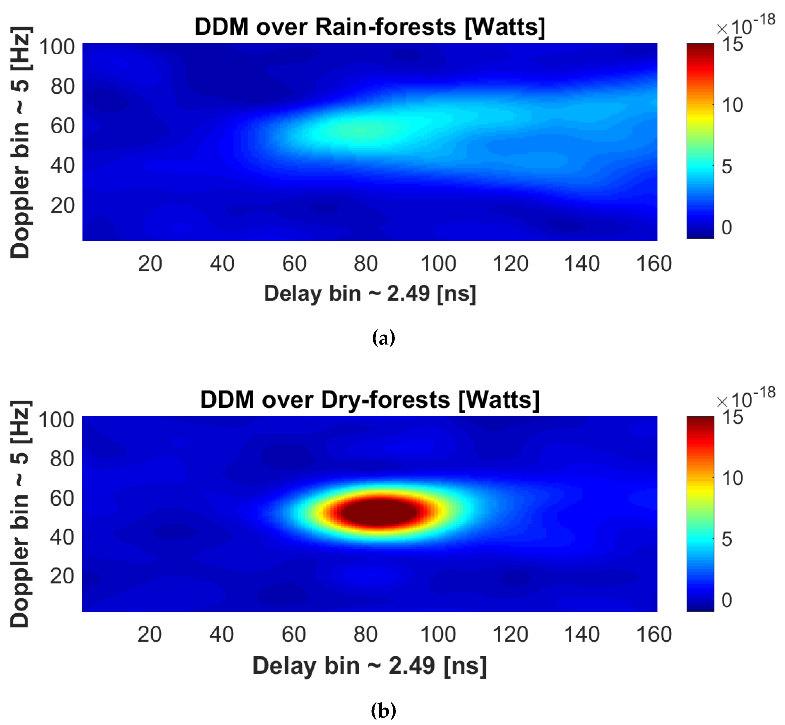
- What is the DDMs’ response to the interaction of GNSS signals with tropical forests?
- What is the GNSS signals saturation level (if any) over tropical forests?
- What is the optimum GNSS satellites elevation angle for biomass estimation over tropical forests?
This work can be understood as a follow-on study of the sensitivity analysis performed in [17]. Here, the main interest is on the sensitivity of and to AGB over tropical forests as a function of CH, , and . The study in [17] was focused on the analysis of the relationship between and the normalized first Stokes parameter over a wide variety of target areas. The “tau-omega” model was found to properly fit this relationship. Several improvements have been introduced: (a) the use of raw DDMs, (b) signal calibration, and (c) the use of several observation geometries. This paper is organized as follows. Section 2 motivates the use of L-band bistatic radar for biomass studies. Section 3 describes the selected observables and the methodology. Section 4 analyses the sensitivity of CyGNSS to AGB, including a comprehensive interpretation of the experimental results. The main conclusions are included in Section 5. Information about test sites and reference data is included in Appendix A and Appendix B, respectively. Finally, Appendix C includes supplemental information for the evaluation of results in Section 4.
2. Exploiting CyGNSS for Biomass Monitoring
2.1. Background
The CyGNSS mission (down looking antenna gain ~ 14.5 dB, LHCP) was first proposed for ocean wind speed estimation over tropical cyclones using GPS L1 C/A signals of opportunity. The orbital configuration of each CyGNSS satellite is a circular Low Earth Orbit (LEO) with a height ~ 500 km and an inclination angle of ~ 35°. Each single Delay Doppler Mapping Instrument (DDMI) [12,14] aboard the 8 CyGNSS microsatellites collects forward scattered signals along four specular directions (elevation angle of the incident wave equals elevation angle of the reflected wave ; = = ) corresponding to four different transmitting GPS spacecrafts, simultaneously (Figure 1). As such, CyGNSS allows one to sample the Earth’s surface along 32 tracks simultaneously, within a wide range of satellites’ elevation angles ~ [20, 90]° over tropical latitudes ~ [−40, 40]°.
The retrieval of geophysical parameters from CyGNSS requires that the DDMI payload cross-correlates directly the collected signals against a known replica of the GPS L1 C/A code, after compensating for the Doppler shift [8,12,14]. Consequently, 32 complex reflected DDMs are generated on-board at a time, using a short coherent integration time ~ 1 ms. Complex DDMs are incoherently averaged along ~ 1 s to finally generate the so-called power DDMs .
Power DDMs can be modelled using geometrical and scattering related parameters as follows [40]:
where is the power of the RHCP transmitted signals, ~ 19 cm is the wavelength of the signals at L1, and are the transmitting and receiving antenna gains, , and are the ranges from the transmitter and the receiver to the specular point, respectively, is the Woodward Ambiguity Function (WAF), is the delay of the signal from the transmitter to the receiver, is the Doppler shift of the reflected signal, is aimed to compensate the Doppler shift of the signal, is the bistatic scattering coefficient at LHCP, and is the positioning vector of the scattering point.
The bistatic scattering coefficient is defined as follows [41]:
where and are the coherent and the incoherent scattering terms, respectively. describes scattering properties of the surface and the vegetation, i.e., volume scattering. depends mainly on surface properties and it has a significantly narrower (practically, a delta function) power distribution over scattering angles than . Consequently, DDMs consists on a sum of two terms, as follows [28,42,43]:
accounts for coherent reflections, while is responsible for the diffuse scattering. The relative portion of both components mainly depends on the coherent integration time , the observation geometry, and both the dielectric and structural properties of the scattering media.
Several works found a transition from incoherent to coherent scattering regime over the ocean surface [43,44], where is dominant for high [45]. Theoretical simulations have been carried out to evaluate the behavior of the incoherent reflected power as a function of [45]. It was stated that decreases ~20% when decreases from ~90° to ~50°. Over land surfaces, global scale results [46] have shown that decreases with decreasing down to ~55°. This empirical observation was justified because of the effect of the incoherent scattering term . On the other hand, increases for lower because of the increasing signal coherence.
The reflectivity accounts for contributions from both coherent and incoherent scattering terms along both angular ranges. The most relevant difference between both scattering terms is on the combination of the electromagnetic field vectors. is the result of the coherent combination of the signals reflected on individual facets within the first Fresnel zone. comes from the random combination of electromagnetic signals scattered within the glistening zone that add together at the GNSS-R receiver. When the combination is fully coherent, accounts for all the reflected power. In the occurrence of diffuse scattering, the random signs of the electric field cross-products cancel out , and the reflected power is provided by . The changes in the angular evolution of depend on the dominant scattering mechanism.
2.2. Motivation
It is hypothesized that GNSS-R measurements have a certain sensitivity to biomass over tropical forests (Figure 2) and this sensitivity can be higher than that of current SAR missions. This hypothesis is based on the following statements: (a) The backscatter intensity measured by monostatic SAR increases with biomass up to a saturation level AGB ~ 100 ton/ha. (b) L-band GNSS signals can partially penetrate the vegetation cover because of the semi transparency of the vegetation at low frequency bands. (c) The bistatic scattering pattern of the coherent surface scattering component follows a delta function along the specular direction, while the incoherent scattered signals spread along all other directions. (d) The coherent component can be higher than the incoherent one even from a space-borne platform.
includes coherent scattering from the surface. It can be expressed analytically as follows [47]:
where is the LHCP Fresnel reflection coefficient, is the signal angular wavenumber, is the surface height standard deviation (related to surface roughness), and is the transmissivity of the vegetation:
where is the Vegetation Optical Depth. is an index of leaf and woody biomass that is used to parameterize absorption effects. data derived at L-band are better correlated to AGB and CH than C-band data because of the higher signal penetration depth at lower frequency bands [48]. C-band is only sensitive to top canopy layers, while L-band is sensitive to the canopy from top to bottom layers [48]. Increasing levels of biomass belong to higher signal attenuation effects. On the other hand, optically derived vegetation parameters, such as, e.g., NDVI are only correlated with green leaf material. Tropical rainforests are characterized by wet biomass and the impact of signal attenuation through the vegetation cover is thus higher than scattering effects [49]. This attenuation becomes higher for decreasing because of the larger signal path along the vegetation cover. The impact of on is twofold. On one hand it influences the Fresnel reflection coefficient, and on the other hand it influences the exponential decaying factor in Equation (4). For a totally flat surface, the root mean square of the surface height variation is zero, and equals the square of the amplitude of the Fresnel reflection coefficient. is constant for > 40° and it decreases significantly for lower angles [27]. However, the exponential factor increases significantly with lower . As a consequence, increases at grazing angles [46].
Finally, it is worth commenting that can be assumed to be roughly independent of the platform’s height in a LEO scenario because . suffers lower free space losses than , following the classical bistatic radar equation.
includes two main contributions: (a) surface scattering over areas with moderate to high roughness (small-scale roughness) and topography, and (b) volume scattering [29] from the vegetation cover including leaves, branches, and trunks. The impact of double bouncing scattering can be assumed to be negligible because the LHCP down looking antennas filter out the RHCP component of the total scattered electromagnetic field. The polarization of GNSS signals changes from RHCP to LHCP after direct scattering. However, they become RHCP after double reflections, first from RHCP to LHCP and then from LHCP to RHCP.
3. Methodology
3.1. Definition of the Selected CyGNSS Observables
CyGNSS Level 2.1 Science Data Record [14,37,38] was selected for this study. The original data were first filtered out using an equivalent “CyGNSS overall quality flag” over land surfaces to improve the quality of the observables. Reflected delay waveforms were obtained from the original DDMs at zero Doppler frequency:
The delay bin resolution of the original 17 lag waveforms is ~0.2552 GPS C/A chips. A re-sampling and interpolation of the resulting 1700 lag waveforms was performed using a spline method [50] to increase the accuracy of the waveforms, before applying the algorithms to extract the observables. Several observables were considered to evaluate the sensitivity of and the volume scattering term to forests biomass.
The trailing edge width was defined as the lag difference between the 70% power threshold of the high-resolution waveforms and the corresponding maximum power of the waveforms [13]:
Different power thresholds were tested. The 50% power threshold was found to cut off some lags when this threshold was out of the original 17 lag waveforms. On the other hand, the 90% power threshold provided a lower dynamic range as compare to the 70%. The incoherent scattering term is the main contribution to , while both the coherent and the incoherent scattering terms significantly contribute to the peak power of the waveforms . are composed of both coherent and incoherent scattering terms over tropical forests. The width of these power waveforms depends on the scattering properties, in a differentiated manner depending on the coherent-to-incoherent scattering ratio. The width is expected to be small if the ratio is high because of the strong power contribution of the coherent term to the peak of the power waveforms.
The reflectivity is estimated as the ratio of the reflected and the direct power waveforms peaks, after compensating for the noise power floor and the antennas’ gain patterns as a function of the elevation angle as:
The antennas’ gain patterns were compensated versus the gain at the corresponding boresight direction (down looking gain ∼14.5 dB, ~62° and up looking gain ∼4.7 dB, ~90°), and the difference of both gains at boresight. The compensation of the antennas’ gain was implemented as a function of . This is relevant for an accurate estimation of because the transmitted signal power depends on , and because both gain patterns have a different relationship with this variable. The CyGNSS Level 1 Science Data Record variables used in this procedure are highlighted here: raw DDM and Zenith Signal-to-Noise Ratio (SNR) for the estimation of and , while Specular point Rx antenna gain for the information of the down looking antenna gain in the direction of the specular point. The up looking antenna is omnidirectional with a gain ∼4.7 dB at boresight and a half power beam width of ∼57°. The noise power floor was estimated as the mean value of the DDM subset where the signal is not present [51]. The delay separation between the DDM subset and DDM peak was at least 0.75 chips, and estimation of was discarded if this distance was shorter than 0.75 chips.
The half power beam width (−3 dB) of each down-looking CyGNSS antenna is ~30°, and the −6 dB field-of-view is ~45°. On the other hand, each antenna pointed to the Earth’s surface with an elevation angle of ~62° (antenna boresight). As such, GNSS signals reflected at low angles down to ~20° can be accurately collected through the main lobe of each antenna.
The nominal mission lifetime is 2 years. This milestone was achieved on March 2019. Experience with CyGNSS wind measurements shows that absolute power measurements is currently one of the challenges of this mission [52,53]. In this work, the direct signal was used to partially improve the estimation of . At present, the mission is operating nominally, and the Automatic Gain Control (AGC) for the Zenith channel was disabled from August 2018. This fact helps to improve the accuracy in the estimation of using Equation (8). On the other hand, could also be inverted from scattering models. However, this approach relies on the assumption that the scattering is totally coherent [51] or totally incoherent [54]. This was the main motivation to use Equation (8) in the estimation of the reflectivity over forests regions, where are composed of both coherent and incoherent scattering terms.
3.2. Auxiliary Forests Vegetation Parameters
The SMAP-Enhanced L3 Radiometer Global Daily 9 km Level L3 SPL3SMP_E Version 1.0 product was used to generate auxiliary vegetation parameters. This product was derived from SMAP radiometer (6 A.M. – 6 P.M. data in different arrays) and ancillary data over the global 9-km Equal Area Scalable Earth (EASE 2-0) grid [55,56,57]. The SMAP L-band mission provides a better signal penetration depth over the vegetation as compared to higher frequency bands. As such, it is an adequate candidate to evaluate the relationship between CyGNSS derived and with AGB, as a function of , , and SMC.
(1) Vegetation Optical Depth (): The retrieval is based on a priori NDVI information obtained from visible-near infrared reflectance data from the NPP/JPSS VIIRS instrument, and land cover type assumptions [55,56,57]. It is used to retrieve the transmissivity of the vegetation as an estimation of the attenuation of the electromagnetic signal through the vegetation layer. SMOS-derived has been also used in, e.g., [58].
(2) Polarization Index (): It is defined as the difference between the microwave radiometric brightness temperatures at V-pol and H-pol , normalized to their average value as follows [59,60,61,62]:
normalizes the measurements of the brightness temperatures and it is independent of the physical temperature of the surface. The potential sensitivity of to dense forest canopies is based on the assumption that V-polarized emission from soil is attenuated by vegetation, which, on the other hand, emits much less polarized radiation depending on the amount of biomass. This parameter was found to decrease when the biomass increases, independently of the crop type. The performance over tropical forests is evaluated here.
(3) Soil Moisture Content (SMC): The retrieval of SMC is based on the use of the V-pol single channel algorithm [55,56,57] only when favorable surface conditions appear at a given grid cell. Corrections for surface roughness, effective soil temperature, and Vegetation Water Content (VWC) were also applied.
3.3. Strategy
and were classified into different groups according to different ranges of the satellites’ elevation angles in steps of ~10° from ~90° to ~20°. is an important parameter that remarkably affects the ratio of the coherent to incoherent scattering components. The contribution of the topography to the incoherent scattering term was partially filtered out to evaluate only the effect of the volume scattering term. In so doing, only pixels over the surface with a Terrain Ruggedness Index (TRI) lower than ~ 15 were considered [63,64]. This threshold was found, empirically, to limit the effect of topography. Several TRI thresholds were tested. It was found that levels higher than ~ 15 significantly increase the spreading of the . On the other hand, there is a remaining incoherent scattering contribution due to the small-scale surface roughness. However, the coherent scattering term largely overpass the incoherent scattering term associated to the small-scale roughness over land surfaces [28,42,47]. Topography is an important factor that disturbs because the local surface slopes modify the size of the scattering area [65].
Quantifying and analyzing the relationship between and against AGB and CH is the main focus of this work. In so doing, SMAP-derived , , and SMC products were also used to further analyze the results. A common grid was thus required, because of the variety of products with different footprint sizes and spatio-temporal sampling characteristics. A 0.1° × 0.1° latitude/longitude grid was selected. All products were averaged using a moving window of 0.2° in steps of 0.1°. The spatial resolution is ~ 20 km × 20 km at equatorial latitudes, which is wide enough to account for the across-track spreading ~20 km of the DDMs due to . The ultimate resolution at a cell center is ~ 20 km × 20 km because multiple satellites overpasses with different orientations were considered. This grid also allows us to account for . This term is limited by the along-track resolution ~7.6 km, related with the orbital motion and the incoherent integration time ~1 s. Finally, it is worth pointing out that this strategy provides a filtering of potential fluctuations of and due to remaining (after quality flags removal) noise sources, such as Attitude Determination and Control Subsystem (ADCS), the geolocation of the nominal specular reflection points, and the use of eight different DDMs sources (eight distributed microsatellites) in the moving averaging filter.
The selected temporal window was 6 months (01/08/2018 to 31/01/2019). This temporal length is large enough to provide statistically significant results. This specific time period was selected because the AGC was disabled on July 2018, so as to improve the performance in the estimation of using Equation (8). The temporal length was selected as large as possible at the time of starting this work because this study is not focused on the analysis of potential temporal fluctuations of different geophysical parameters. The temporal variations of AGB and CH during this period were assumed to be negligible.
4. Performance Analysis
4.1. Introduction
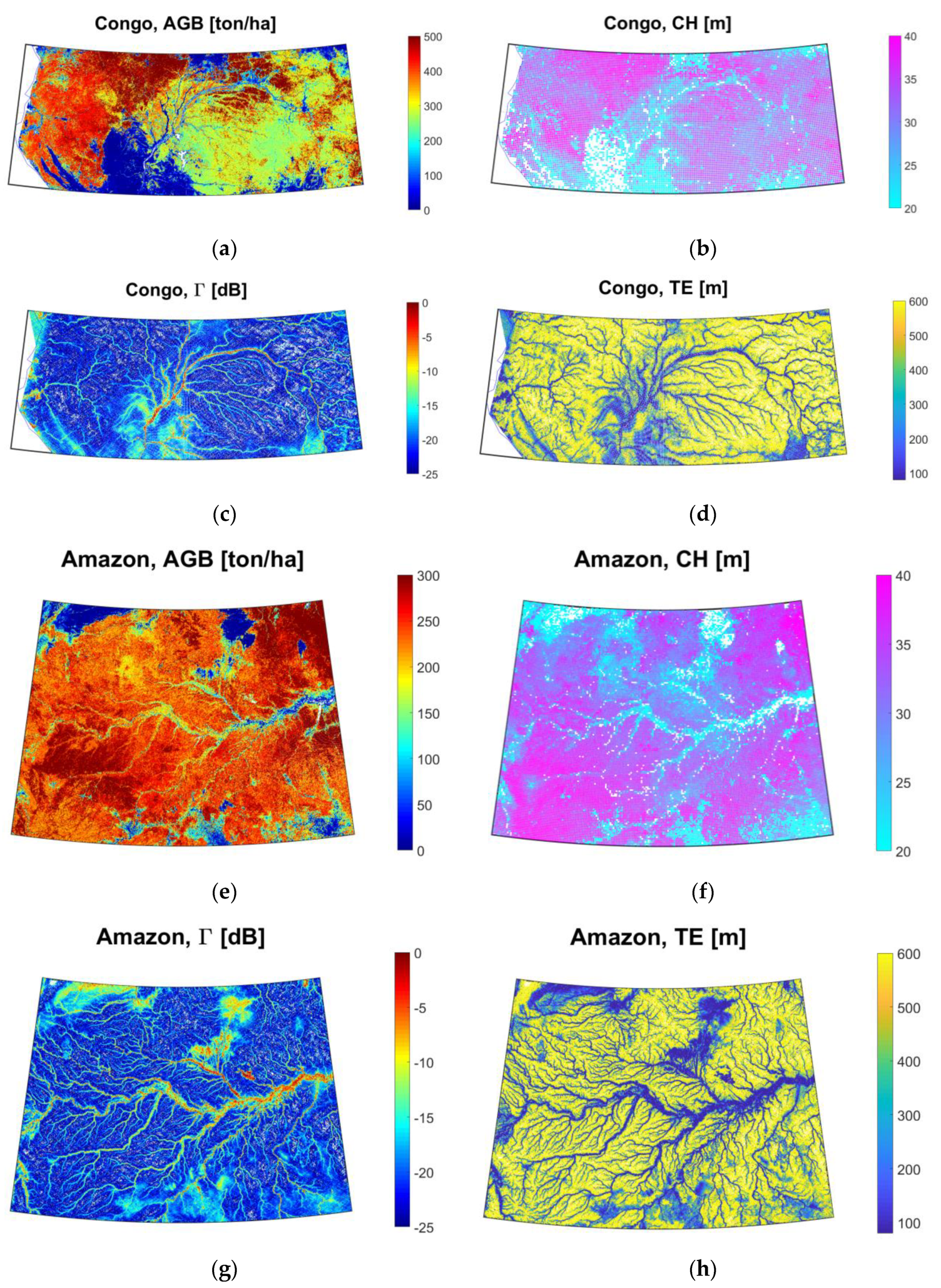
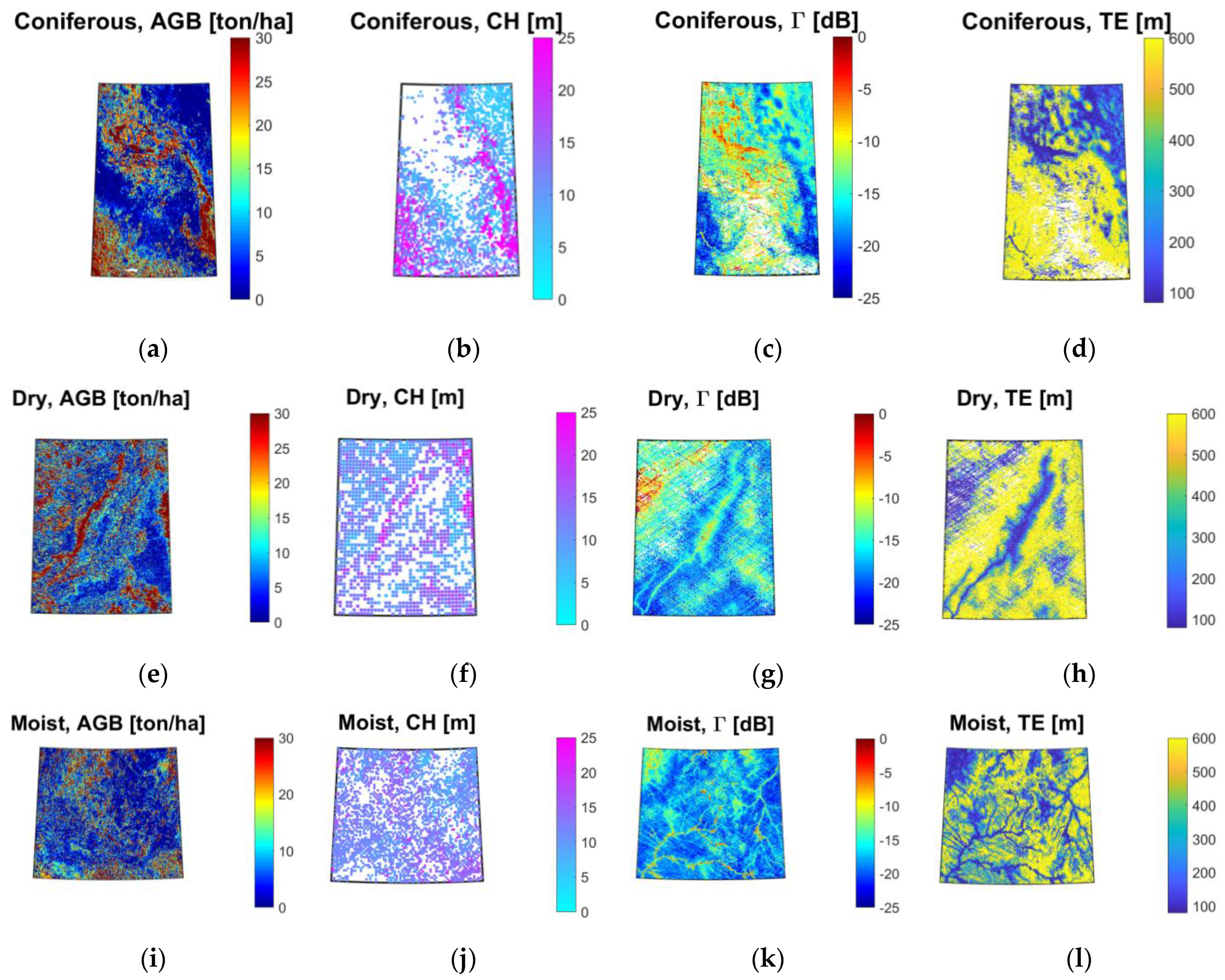
CyGNSS-derived and were used in this study to improve our understanding in the performance of GNSS-R for biomass studies (Figure 3, Figure 4, Figure 5, Figure 6, Figure 7 and Figure 8). The analysis was performed over different types of forests, such as Congo rain (Figure 3a–d, Figure 4a–d, and Figure 5a–d), Amazon rain (Figure 3e-h, Figure 4e-h, and Figure 5e-h), coniferous (Figure 6a–d, Figure 7a–d, and Figure 8a–d), dry (Figure 6e-h, Figure 7e-h, and Figure 8e-h), and moist (Figure 6i–l, Figure 7i–l, and Figure 8i–l) tropical forests. These target areas were selected so as to cover a wide variety of forests on a pantropical scale.
AGB and CH data were obtained from the Avitabile et al. product [39] and the ICESat-1/GLAS space-borne instrument [3,6], respectively. Both biomass references were displayed over the specific target areas, enabling a first qualitative evaluation (Figure 3 and Figure 6). A certain correlation of and with AGB and CH was found over the selected study sites (Table 1). This correlation improves over more dense forest canopies. decreases with increasing biomass levels. On the other hand, the spreading of increases with increasing levels of biomass. Avitabile’s map and CyGNSS sampling properties show a good performance, while GLAS-derived CH data are provided with less spatial density. This observation motivates the selection of AGB from Avitabile et al. as the main biomass reference. CH was used as an auxiliary product to assess the potential impact of this term in the interaction of GNSS signals with the vegetation.
4.2. Sensitivity Analysis as a Function of the Elevation Angle
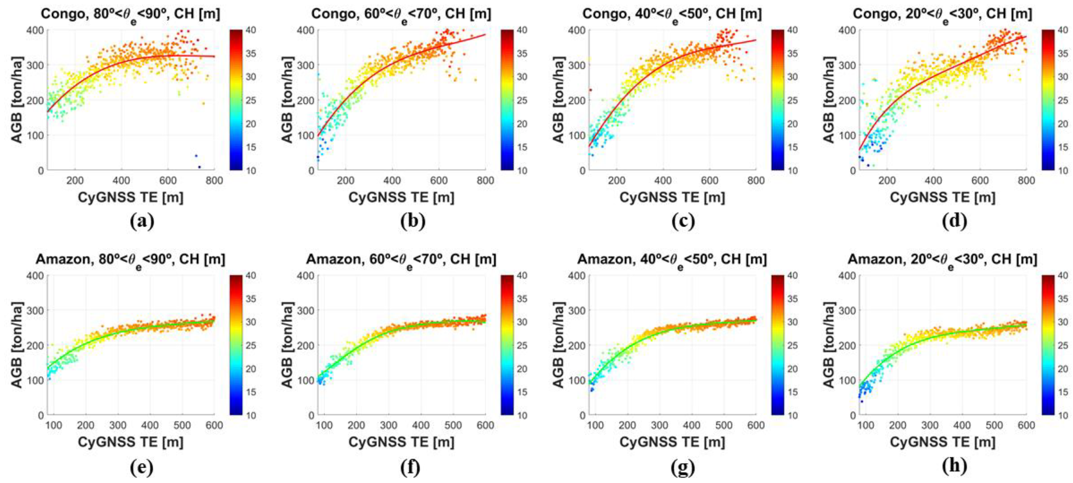
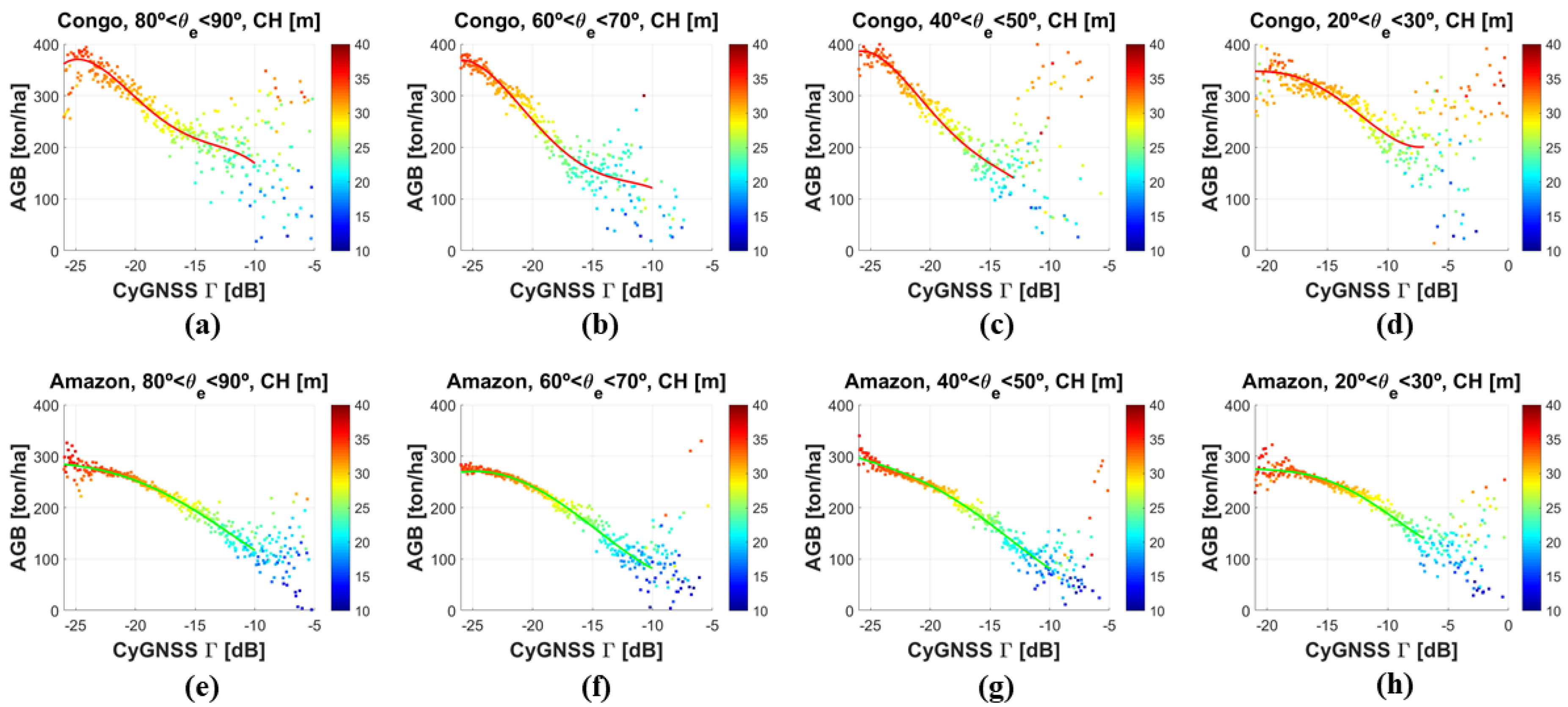
Figure 4, Figure 5, Figure 7 and Figure 8 show the scatter plots of and with AGB over Congo rain (Figure 4a–d and Figure 5a–d), Amazon rain (Figure 4e–h and Figure 5e–h), coniferous (Figure 7a–d and Figure 8a–d), dry (Figure 7e–h and Figure 8e–h), and moist (Figure 7i–l and Figure 8i–l) tropical forests. These plots are depicted as a function of CH. They were computed using the mean values of the biomass reference data in steps of ~ 1 m and ~ 0.05 dB. The values of these steps were found empirically. This strategy allowed us to filter noise at a pixel level, such as speckle in , and potential errors in GLAS-derived AGB. On the other hand, it provided enough sampling density to compute the correlation coefficients, i.e., Spearman for rainforests, and Pearson for other forests (Table 1). Different steps were also tested. Decreasing values of these steps belonged to a noisier behavior in the scatter plots, while increasing values reduced sampling density. The extension of the target areas is large, providing enough data. The errors were assumed to be randomly distributed. Thus, noise could be reduced after averaging, so as to find the underlying relationship between CyGNSS observables and AGB. This work is focused on the analysis of this empirical relationship on a regional scale. The correlation between the mean values of both CyGNSS observables and AGB is clearly visible. Increasing levels of AGB belongs to decreasing and increasing .
Speckle is a source of noise that involves diffuse scattering. If the scattering medium is rough with respect to , the different heights of the scatterers over the glistening zone will randomly shift the phases of the GNSS signals. Some of these paths will destructively interfere and others will constructively interfere. Thus, the signal power level as measured by CyGNSS will change randomly. From this point, it can be stated that the SNR of the reflected signals is affected by tropical forests. The strategy described previously was applied to mitigate this effect. At the same time, the AGB reference data could potentially have some errors because this dataset is derived from CH data and assumed continental allometric relationships. Nonetheless the validation of Avitabile’s map [39] shows a lower root mean square error (RMSE) (reduction down to ~74%) and bias (reduction down to ~153%) than both original datasets [66,67] over all the continents. An interpretation of the results is provided for each study site:
(1) Tropical rainforests (Figure 4 and Figure 5): The empirical relationships of and with AGB were fitted by empirically derived polynomial functions (Table 1) at different angular ranges ~[80, 90]°, ~[60, 70]°, ~[40, 50]°, and ~[20, 30]° over Congo (Figure 4a–d and Figure 5a–d) and Amazon (Figure 4e–h and Figure 5e–h). The first derivative of these functions was computed at different mean levels of AGB in steps of ~50 ton/ha, for different angular ranges (Table A1, Table A2, Table A3 and Table A4). The values of the derivative reduce with increasing AGB levels. Uncertainties in AGB estimation were computed as the values of the first derivatives times the uncertainties in the GNSS-R observables. This point is translated into smaller uncertainties in the estimation of AGB with increasing biomass levels. A budget (ignoring noise) is provided assuming uncertainties of, e.g., ~ 1 m and ~ 0.1 dB (Table A5, Table A6, Table A7 and Table A8).
In this work, the main interest is in the sensitivity, ignoring noise in the measurements when observations deviate from the fits [68]. As such, at a first order, the required GNSS-R sensitivity and the AGB uncertainties are related by the first derivative of the fitting functions [69]. These results suggest that different types of forests have a different response. As such, different models should be applied to retrieve biomass at each type of forest.
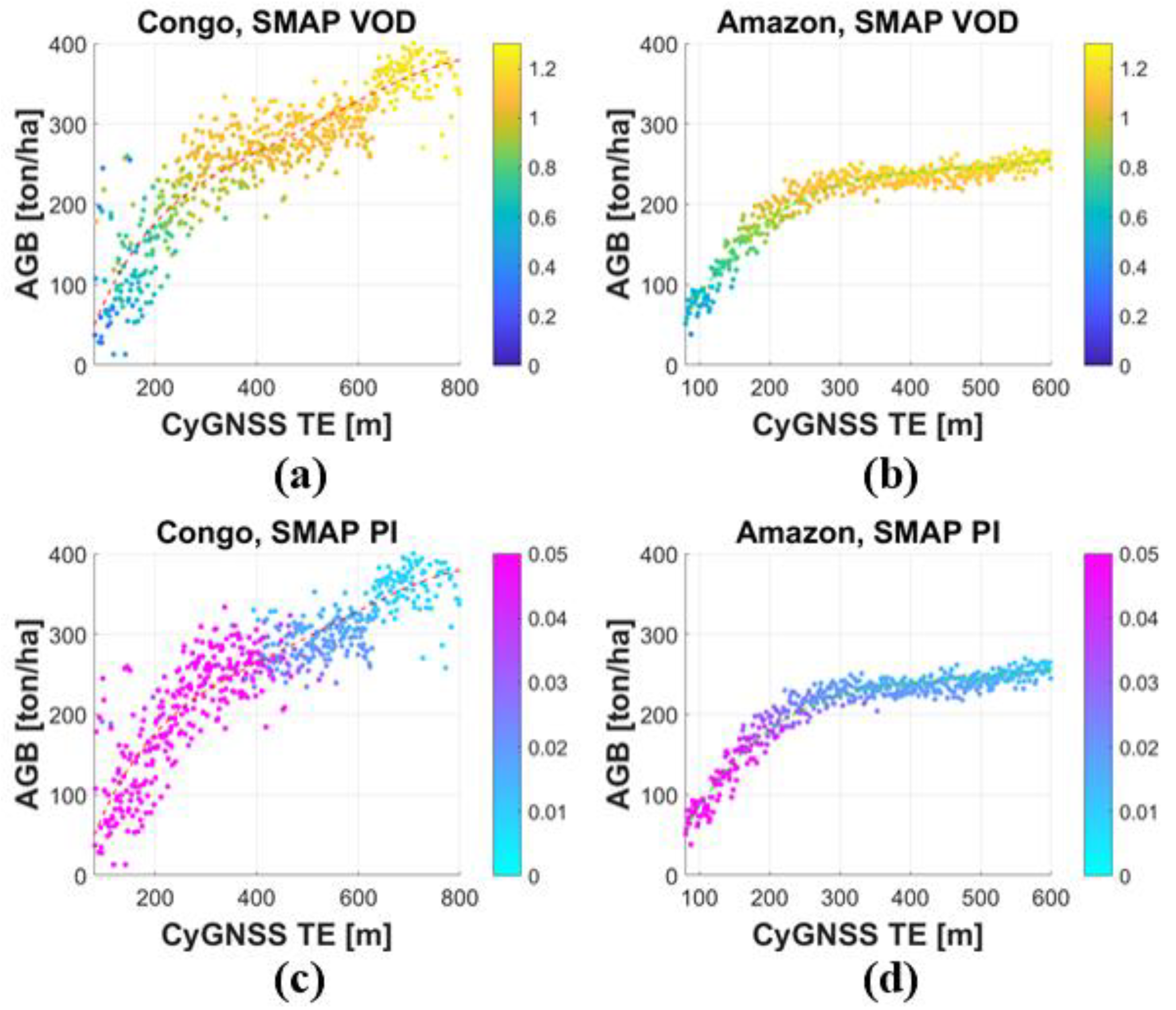
Figure 4 and Figure 5 show that increases with increasing AGB up to ~ 800 m over Congo (Figure 4d) and ~ 600 m over Amazon (Figure 4e–h). This experimental evidence is justified because, for increasing vegetation levels (Figure A1a,c), (a) a higher volume scattering term in increases the tail of , and (b) the coherent scattering term is gradually more attenuated. On the other hand, the measurable AGB dynamic range increases with decreasing , from ~140 ton/ha at ~[80, 90]° to 300 ton/ha at ~[20, 30]° over the Congo target area, while it increases from ~ 140 ton/ha at ~[80, 90]° to 170 ton/ha a ~[20, 30]° over the Amazon site. The measurable AGB range is a function of because of the impact of the different scattering mechanisms at different . The coherent scattering increases at grazing angles, belonging to a higher measurable AGB dynamic range, as compared to a Nadir looking configuration. The improved measurable dynamic range at lower angles is explained because of the higher coherent reflectivity at this geometry Equation (4). This scattering property belongs to an increment of the SNR dynamic range, which in turn improves the sensitivity of to the attenuating cover. Coherence effects could also appear after scattering over the vegetation cover if the coherent integration time would set to be long enough, e.g., ~ 20 ms [27,28,33], so as to filter out the noise and the volume scattering term. However, the volume scattering term is high for lower integration times, e.g., ~ 1 ms.
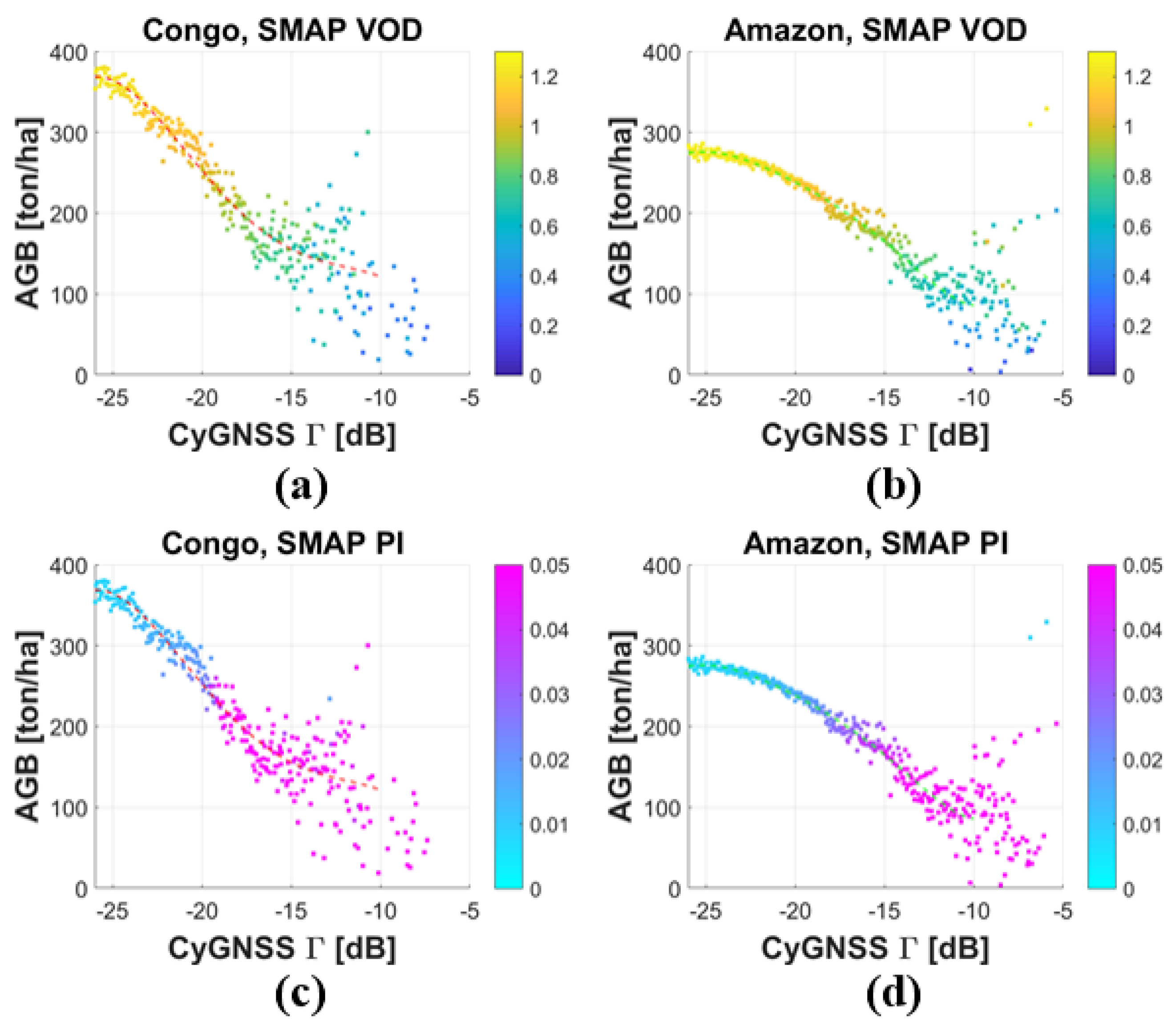
gradually decreases down to ~ −25 dB with increasing AGB because of the increasing attenuation of the GNSS signals along the vegetation cover (Figure 5). The measurable AGB dynamic range first increases from ~[80, 90]° to ~[60, 70]°, and later it reduces with decreasing angles from ~[60, 70]° to ~[20, 30]°. On the other hand, is significantly stronger at ~[20, 30]° than at higher observation angles. This is a symptom that the coherent scattering term is dominant at grazing geometries, even over tropical rainforests [46]. The coherent scattering term is mainly associated with surface scattering. As such, the sensitivity of to AGB reduces when is dominant. Indeed, it is found that the RMSE of the scatter plots increases with increasing levels. Potential fluctuations of surface properties have a stronger impact at this geometry (Figure 5). With this respect, the performance of is better than . The information in is poorly related to biomass when is dominant. However, the higher SNR dynamic range is linked to a higher dynamic range, which in turn increases the sensitivity of to AGB, although the sensitivity of is poor. These observations suggest that the sensitivity of to forests canopies improves when the incoherent scattering term is dominant over the coherent one [46]. Indeed, the highest AGB dynamic range appears at ~[60, 70]°. The interpretation is two-fold: (a) a larger signal propagation path through the vegetation, as compared to that corresponding to higher , improves the sensitivity to biomass, and (b) the coherent scattering term starts to be dominant for angles lower than ~ 60° [46]. A complementary description of the impact of can be found in [46].
Overall, it is also found that the dispersion in the scatter plots is very high over the strongest levels of , where surface reflectivity starts to play an important role in the overall reflectivity. This significant dispersion is related to the fluctuations of certain surface properties, depending on the surface area under consideration. This dispersion increases for grazing angles, which suggests that surface properties such as rivers start to play an important role. As such, appears quite high even for high AGB levels.
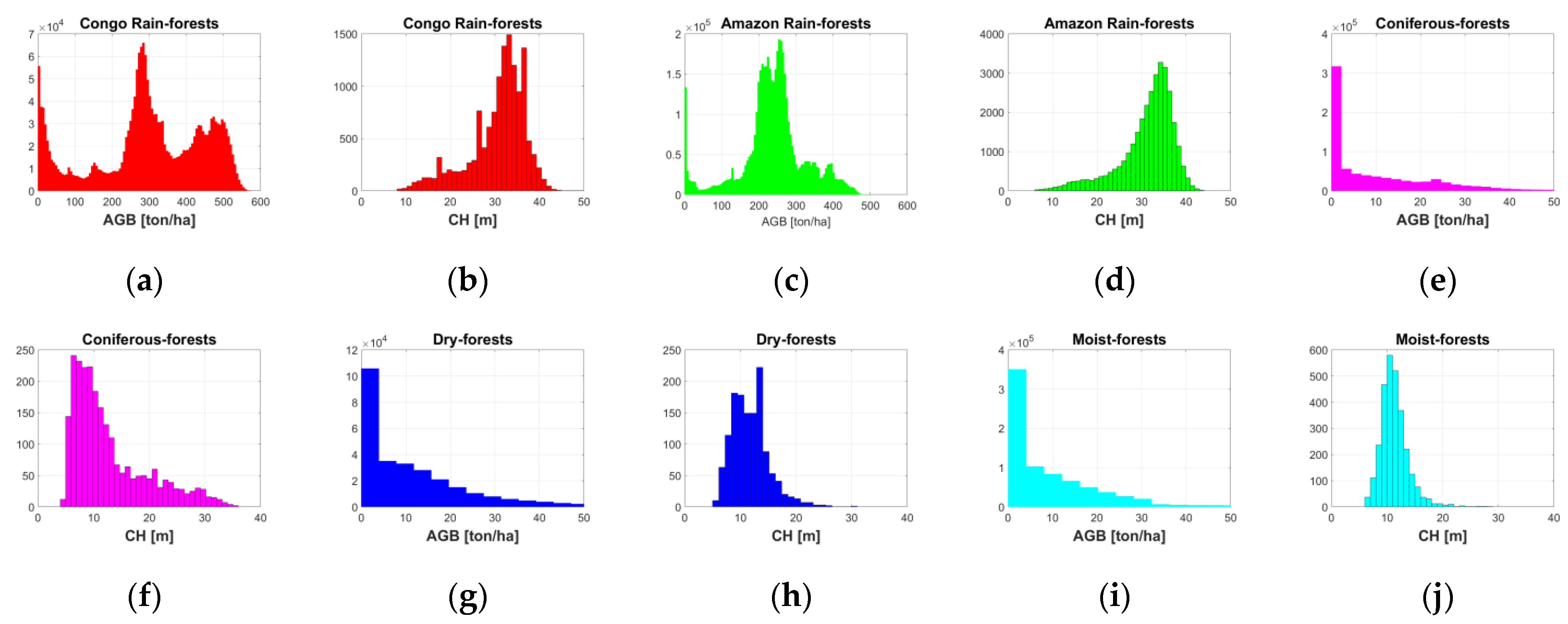
The sensitivity over Congo rainforests shows a higher angular variability than over the Amazon. This experimental evidence could be linked to different structural properties of the vegetation cover. The AGB distribution over the Amazon is a bimodal one with the two peaks at ~200 and ~250 ton/ha (Figure A1c). The re-radiation pattern could have isotropic properties because of the small separation between both modes. This characteristic could explain the small angular variability of the sensitivity. On the other hand, a bimodal distribution is also found over the Congo (Figure A1a). The two modes are much more differentiated, with peaks at ~300 and ~500 ton/ha. It is hypothesized that this characteristic could belong to a much more complex structure of the canopy layer, and a higher angular variability.
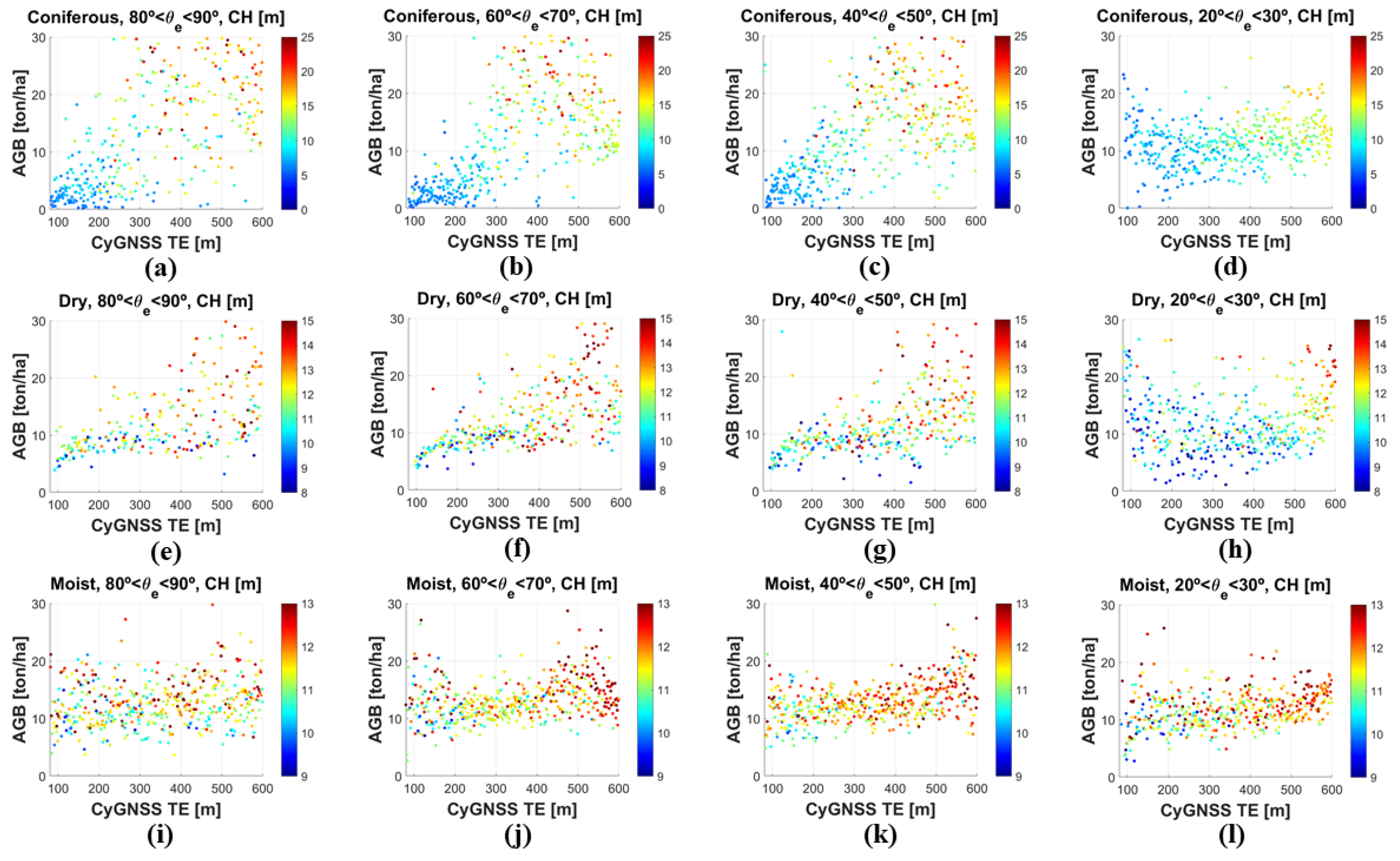
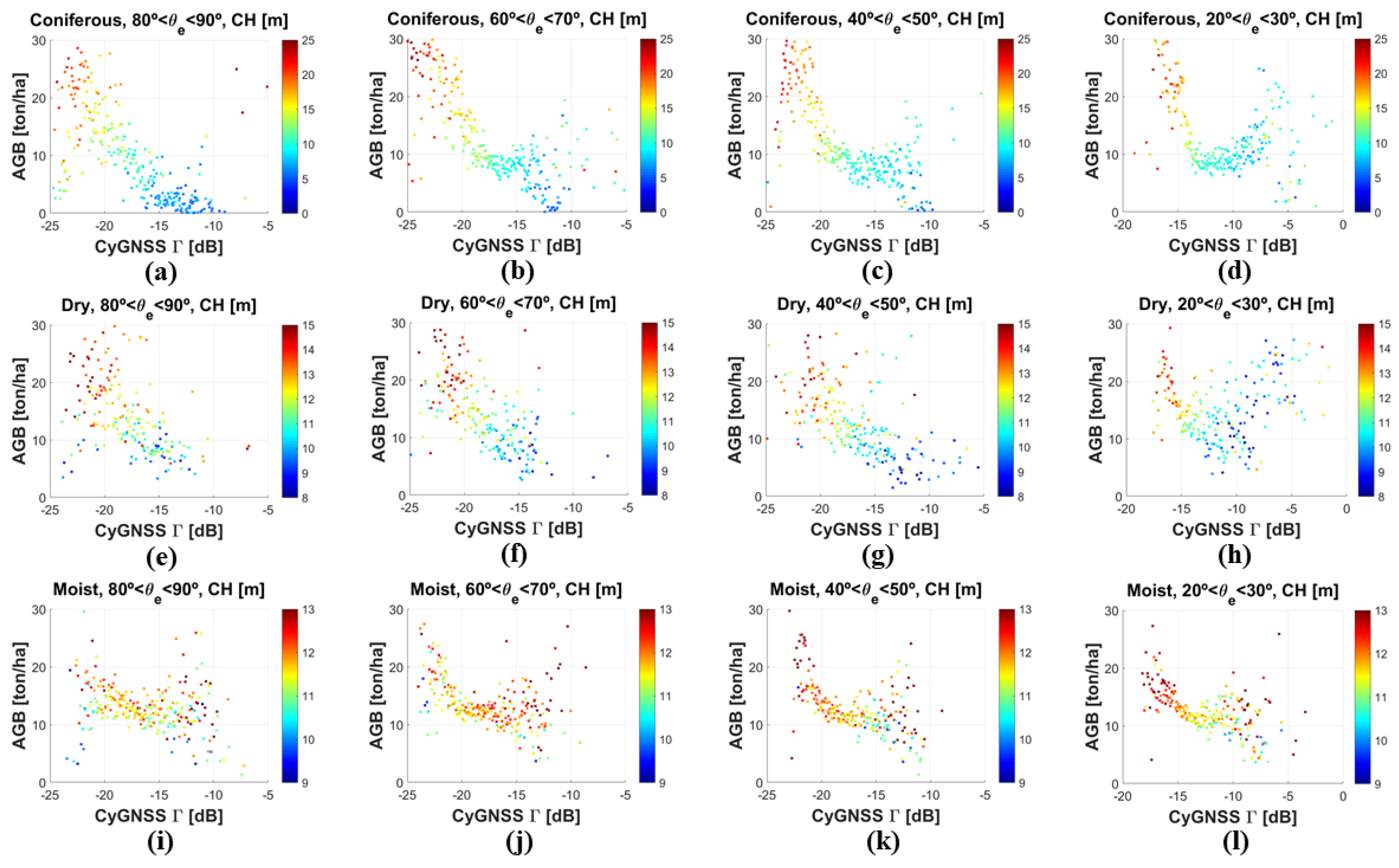
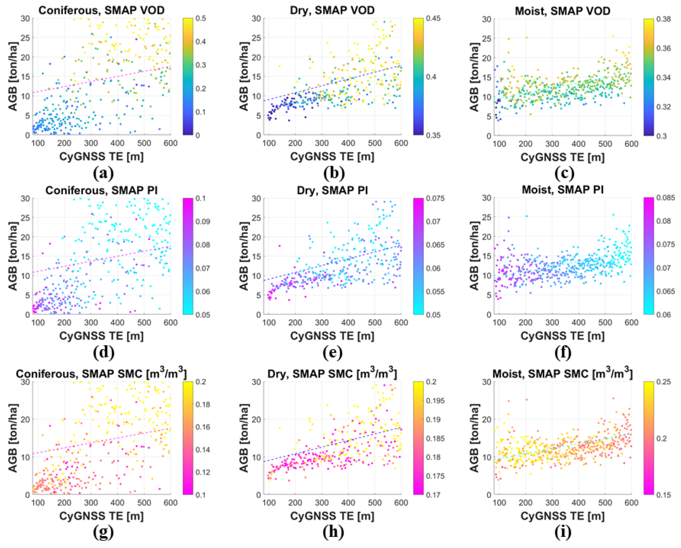
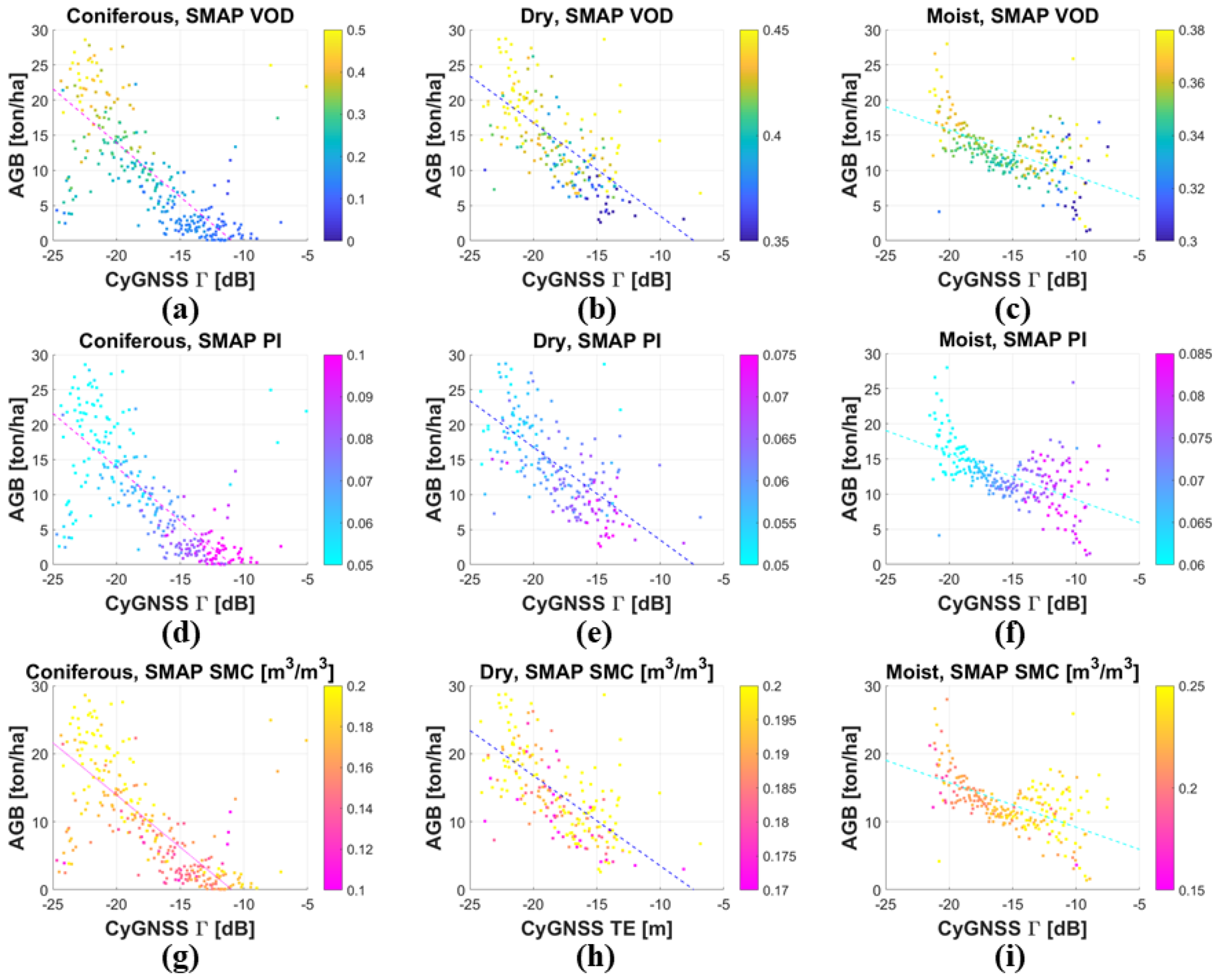
(2) Coniferous, dry, and moist tropical forests (Figure 7 and Figure 8): The functional correlations of AGB with (Figure 7) and (Figure 8) can be fitted by empirically derived 1st order polynomial functions. Table 1 summarizes the statistics of these fits at different angular ranges ~[80, 90]°, ~[60, 70]°, ~[40, 50]°, and ~[20, 30]°, over coniferous (Figure 7a–d and Figure 8a–d), dry (Figure 7e–h and Figure 8e-h), and moist (Figure 7i–l and Figure 8i–l) forests. A distinguished characteristic of these forests is the low level of AGB, combined with moderate to high levels of CH (Figure A1e–j). These forests are presented following a decreasing CH level from coniferous (Figure A1f) to moist forests (Figure A1j).
The assessment using and shows that the maximum correlation coefficients and slopes of the linear regressions (Table 1) appear gradually at decreasing with decreasing CH levels: ~[80, 90]° over coniferous, ~[60, 70]° over dry, and ~[40, 50]° over moist forests (Table 1). The angular differences are small. The RMSE is high even for low AGB levels. A reasonable justification is provided, despite the fact that these aspects complicate the interpretation of the results.
Larger signal propagation paths through the vegetation cover are required to increase the sensitivity with decreasing CH levels. On the other hand, the surface contribution partially masks the vegetation effects at grazing geometries. This latter aspect can be observed more clearly at ~[20, 30]°, where the correlation coefficients with AGB are quite low (Table 1). This behavior is different to that over rainforests, because low AGB levels belong to a stronger contribution of surface scattering in . Finally, it is worth pointing out that the correlation of AGB with is much higher than with . This observation is also justified because of the dominant effect of surface scattering (Figure 2). On the other hand, the influence of volume scattering is low because of the low AGB levels. This point is translated into lower correlation coefficients with , because the sensitivity of to AGB is almost negligible in this scenario. Over forests with low AGB ~ < 40 ton/ha, the soil surface contribution to the case of GNSS-R is dominant. This explains the lower spreading of the waveforms, as compared to rainforests (Figure 2). In the latter scenario, the volume scattering is very strong.
4.3. Evaluation with SMAP-derived VOD, PI, and SMC
At present, most of biomass monitoring studies are based on the use of visible and infrared indices. However, these types of measurements are only sensitive to the upper canopy layers and they additionally suffer from weather conditions and clouds. On the other hand, this study is based on measurable biomass parameters (AGB, CH). These considerations motivate to complement this work with microwave radiometry-derived parameters, such as and . There is an increasing interest on the use of both parameters to estimate some vegetation properties, such as VWC and AGB [58,59,60,61,62]. Additionally, SMC is considered over coniferous, dry, and moist forests, because of the potential impact of this parameter in the performance of CyGNSS over forests with low AGB levels (Figure A1). Over tropical rainforests, the impact of SMC is assumed to be negligible [24]. As a matter of fact, SMC data are not fully reliable over very dense forest canopies.
The functional relationship of AGB with both and is further evaluated at the specific angular ranges where the optimum performance is found in terms of correlation coefficients and AGB dynamic ranges (Figure 4, Figure 5, Figure 7 and Figure 8). This is a case by case study that depends on the characteristics of each type of forest: Congo rain ( at ~[20, 30]° and at ~[60, 70]°), Amazon rain ( at ~[20, 30]° and at ~[60, 70]°), coniferous ( and at ~[80, 90]°), dry ( and at ~[60, 70]°), and moist ( and at ~[40, 50]°) forests. An interpretation of the results is provided for each target area:
(1) Tropical rainforests (Figure 9 and Figure 10): increases with increasing AGB, so as to provide an estimation of the attenuation by the vegetation cover. The sensitivity of to AGB is high up to AGB ~350 ton/ha ( ~ 800 m and ~ −25 dB) over Congo (Figure 9a and Figure 10a), and up to AGB ~250 ton/ha ( ~ 600 m & ~ −25 dB) over Amazon (Figure 9b and Figure 10b). This sensitivity is qualitatively similar to that of CH (Figure 4d,h and Figure 5b,f). Recently, a good correlation of Soil Moisture Ocean Salinity (SMOS)-derived with CH has also been reported [48,70]. On the other hand, SMAP-derived is linearly related to VWC trough a parameter that accounts for the structural effects of the vegetation cover [55]. As such, it seems reasonable to find this dependence with CH, although VWC is indirectly inferred from NDVI.
Microwave radiometric brightness temperatures, and , depend on frequency, polarization, and the geometrical and dielectric properties of the scattering media. Different polarization characteristics of bare soil and vegetation suggest the potential use of for biomass studies [59,60,61,62]. should gradually decrease with increasing AGB levels because (a) V-polarized emissivity from soil is attenuated by the upwelling vegetation cover, and (b) the radiation component due to forest canopies is roughly unpolarized. Figure 9 and Figure 10 confirm these theoretical expectations. The polarization degree decreases with increasing AGB, without an apparent saturation. Additionally, it is found that takes different values for the Congo and Amazon for a given AGB level. This empirical observation suggests that slightly depends on CH additionally to AGB, at least over tropical rainforests. A similar dependence with CH is also found for .
(2) Coniferous, dry, and moist tropical forests (Figure 11 and Figure 12): A significant sensitivity of is also found for low levels of AGB, over coniferous (Figure 11a and Figure 12a), dry (Figure 11b and Figure 12b), and moist (Figure 11c and Figure 12c) forests. The sensitivity improves with increasing CH levels, from moist to coniferous forests, despite the roughly similar AGB levels (Figure A1e,g,i). On the other hand, also performs well over this type of CH-driven forests (Figure 11d–f and Figure 12d–f). The dynamic range over dry forests ~[0.05 0.075] is slightly lower than over coniferous forests ~[0.05 0.1] because of the lower CH dynamic range (Figure A). At the same time, it is found that is higher over moist forests ~[0.06 0.085] than over dry forests, because of the slightly lower CH levels (Figure A).
The results are independent of SMC over coniferous and dry forests. Over coniferous forests, increasing levels of SMC up to ~0.2 m3/m3 are found for gradually increasing (Figure 11g) and decreasing (Figure 12g). This observation means that CH (Figure A1f) has a higher impact than SMC in both observables, and . An increment in SMC would reduce and increase , in the case that SMC would be dominant. Over dry forests, SMC ~0.18 m3/m3 is quite homogenous along both (Figure 11h) and (Figure 12h) dynamic ranges. As such, changes on and are assumed to be mainly related to the effects of the vegetation cover. Finally, in the case of moist forests, SMC influences (Figure 11i) and (Figure 12i). Increasing levels of SMC up to ~0.25 m3/m3 are found for decreasing (Figure 11i) and increasing (Figure 12i). Even in this scenario, (Figure 11c and Figure 12c) and (Figure 11f and Figure 12f) are found to have a certain degree of sensitivity to canopy forests.
4.4. First Evidences of Biomass Retrieval Using an Empirical Approach
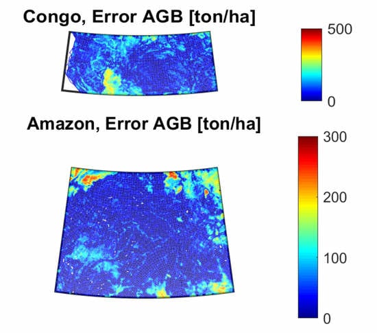
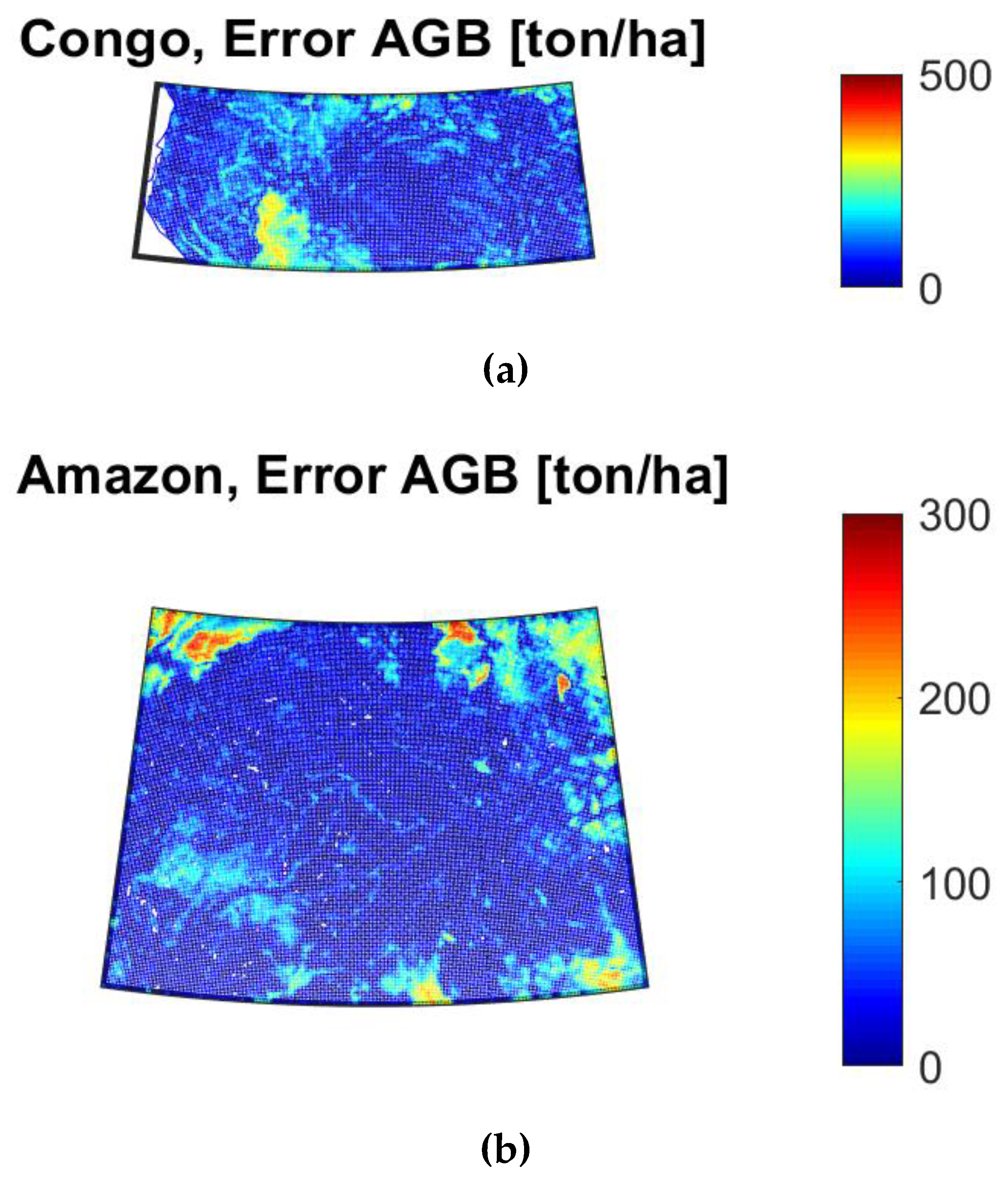
Finally, the ability to retrieve biomass using an empirical approach is evaluated (Figure 13). To do so, the empirically derived polynomial fitting functions corresponding to the relationship between and AGB at low elevation angles ~[20, 30]° are used to provide a preliminary AGB estimation at the two selected test sites over Congo and Amazon tropical rainforests. The percentage of data used as training and validation subsets ranged from 30% and 70%, respectively. On the other hand, the AGB map provided by Avitabile et al. is used as the AGB reference. Small absolute errors in AGB estimation are found except in areas with AGB > ~ 350 ton/ha and in areas with little biomass and the presence of inland water bodies (Figure 3). These promising preliminary results should be further investigated in future works also using ground truth data for validation.
5. Conclusions
Earth-reflected GNSS signals collected in a bistatic radar configuration by CyGNSS, show a significant sensitivity to biomass over rain, coniferous, dry, and moist tropical forests. Future studies with the U.K. TDS-1 mission would help to also cover boreal forests. The sensitivity has been evaluated using several parameters derived from DDMs, as a function of . The optimum results in terms of correlation coefficients and AGB dynamic ranges were found at different angles: Congo rain ( at ~[20, 30]° and at ~[60, 70]°), Amazon rain ( at ~[20, 30]° and at ~[60, 70]°), coniferous ( and at ~[80, 90]°), dry ( and at ~[60, 70]°), and moist ( and at ~[40, 50]°). The SNR reduces at low elevation angles for both direct and reflected signals. However, we use . This observable is more related with geophysical parameters than the SNR. In particular, increases at lower angles because of the lower effective surface roughness at this geometry.
Over rainforests, the optimum geometry for the use of appears at grazing angles because: (a) a higher volume scattering term increases the tail of , and (b) a higher coherent scattering term belongs to an improved sensitivity of to the attenuating cover. On the other hand, the optimum geometry for is found at moderate , when the incoherent scattering term is still dominant and the signal propagation path along the vegetation cover is higher than at a Nadir-looking configuration. Then, the first derivative of the corresponding polynomial fitting functions of the relationship between AGB with and was computed. It was found that there is a certain sensitivity to AGB up to ~350 and 250 ton/ha, respectively, over Congo and Amazon target areas, without an apparent saturation. The first maps of absolute error in AGB retrieval from space using GNSS-R were included, showing a small error. These findings suggest the possibility of accurate AGB retrieval using GNSS-R on-board small satellites such as, e.g., CyGNSS.
Over forests with low AGB ~ < 40 ton/ha, the optimum geometry for the use of both parameters and appears at decreasing with gradually decreasing CH levels. This point is explained because an increasing signal propagation path through the vegetation is required to improve the sensitivity with decreasing CH levels. The correlation coefficients of AGB with are higher than those with . The sensitivity of to AGB is low because of the negligible volume scattering term over these types of forests. In this scenario, the spreading of is low, which reduces the sensitivity of to biomass.
Finally, it is worth pointing out that the application of a moving averaging filter minimizes potential errors in the estimation of due to inaccuracies in the signal calibration. The uncertainty in establishing the relationship between CyGNSS measurables and forest parameters is due to (a) potential errors in CH data derived from GLAS and (b) noise at the pixel level, such as speckle in . Overall, RMSE in the scatter plots increases with increasing biomass levels, while the correlation coefficients increase.
Author Contributions
Conceptualization, methodology, software, investigation, and writing-original draft preparation by H.C.-L.; supervision, by G.L. and M.C. All authors have read and agreed to the published version of the manuscript.
Funding
This research received no external funding.
Acknowledgments
This research was carried out with the support grant of a Juan de la Cierva postdoctoral research fellowship from the Spanish Ministerio de Ciencia e Innovacion, reference FJCI-2016-29356.
Conflicts of Interest
The authors declare no conflict of interest
Appendix A: Study Sites
True rainforests (Figure A1a–d and Figure A2a,b) appear in the latitudinal band Latitude ~ [−10, 10]°. They are a subset of the tropical forest biome that extends within Latitude ~ [−28, 28]°. In this work, tropical rainforests over the Congo (Latitude = [−4, 4]°, Longitude = [9, 28]°) and the Amazon (Latitude = [−10, 5]°, Longitude = [−75, −54]°) basins were selected for an evaluation on a pantropical scale. The mean monthly temperature is over ~ 18 °C along the year and the average annual rainfall is over ~ 1680 mm [71]. Both study sites contain the two major carbon pools on Earth. The dominant International Geosphere Biosphere Program (IGBP) land cover type is evergreen broadleaf forests, which are characterized by wet biomass. This type of biomass is associated with signal attenuation effects [49]. On the other hand, dry biomass is associated with incoherent scattering effects because vegetation albedo is higher over drylands with forests [72]. Albedo is related with land cover type heterogeneity and structural effects of the canopy layer [49]. It is worth noting that both attenuation (linked to vegetation opacity) and scattering (linked to albedo) can be found in a general case. Evergreen broadleaf forests comprise many species with rather unique vegetation structural patterns. They consist of different vertical layers, including overstory, canopy, understory, shrub layer, and ground level. As such, dielectric and structural properties are complex and heterogeneous. The AGB distribution over Congo differs from that over Amazon, although the CH distribution is relatively similar over both sites.
Coniferous tropical forests (Figure A1e,f and Figure A2c) appear mainly in North and Central America. In this work, the selected target area was over Mexico (Latitude = [19, 28]°, Longitude = [−104, −98]°). This type of forest is characterized by low levels of precipitation and a moderate variability in temperature [73]. The dominant IGBP land cover type is woody savannas, which are characterized by diverse species of conifers (firs, pines, spruces, etc). The CH distribution is spread up to ~ 35 m, although the AGB is low ~ < 40 ton/ha.
Dry tropical forests (Figure A1g,h and Figure A2d) appear mostly in tropical and subtropical bands. In this work, the selected target area was over Zambia (Latitude = [−14, −9]°, Longitude = [29, 33]°). These forests are dominated by warm climates. They receive several hundreds of centimeters of rain per year, although they have long dry seasons that can last for several months [74]. Deciduous trees predominate in most of these forests. The CH distribution spreads up to ~ 20 m and AGB is low ~ < 40 ton/ha.
Moist tropical forests (Figure A1i,j and Figure A2e) are discontinuously found over patches on the equatorial belt and between the tropics of Cancer and Capricorn. They are characterized by low variability in annual temperature and high levels of rainfall. Forest composition is dominated by semi-evergreen and evergreen deciduous tree species [71]. In this work, the selected target area was over Brazil (Latitude = [−20, −13]°, Longitude = [−51, −43]°). The CH distribution spreads up to ~17 m and AGB is low ~ < 40 ton/ha.
Figure A1.
Histograms of Avitabile et al. Above-Ground Biomass (AGB) and ICESat-1/GLAS Canopy Height (CH) data over the selected target areas: (a,b) Congo rain, (c,d) Amazon rain, (e,f) coniferous, (g,h) dry, and (i,j) moist tropical. Forests type are classified, as per Global Ecological Zones by the Food and Agriculture Association (FAO) of the United Nations.

Figure A2.
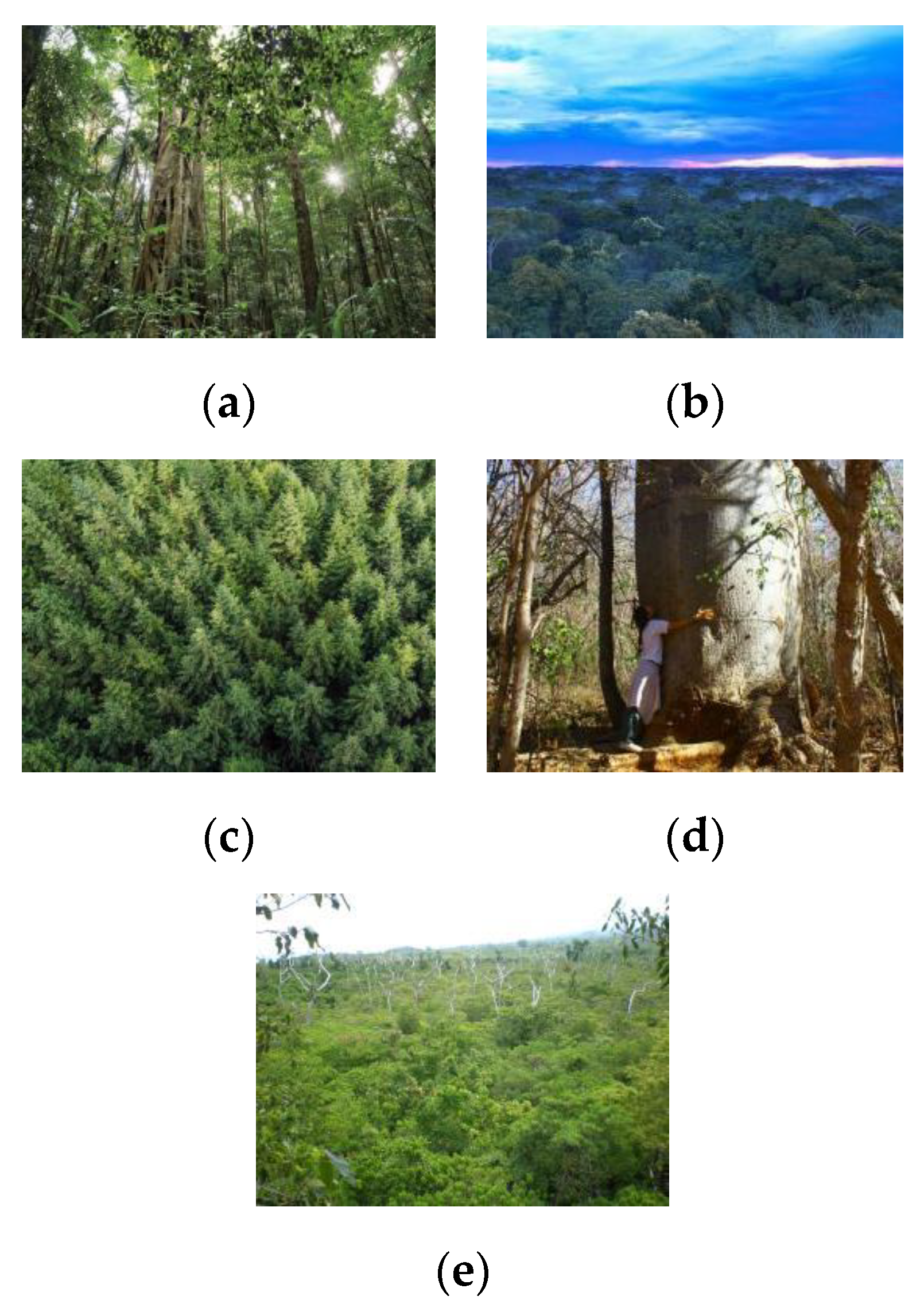
Photos of the selected study sites: (a) Congo rain, (b) Amazon rain, (c) coniferous, (d) dry, and (e) moist tropical forests. Congo rainforests (~2 million km2) [75] contain the highest levels of AGB on Earth [39]. On the other hand, Amazon rainforests spread over ~6 million km2 [76]. The world’s tropical forests store ~ 250 billion tons of carbon.
Figure A2.
Photos of the selected study sites: (a) Congo rain, (b) Amazon rain, (c) coniferous, (d) dry, and (e) moist tropical forests. Congo rainforests (~2 million km2) [75] contain the highest levels of AGB on Earth [39]. On the other hand, Amazon rainforests spread over ~6 million km2 [76]. The world’s tropical forests store ~ 250 billion tons of carbon.

Overall, the selected target areas cover a wide variety of forests at a pantropical scale. Additionally, different surface moisture conditions are expected to be found over different target areas. This aspect was also evaluated in this work.
Appendix B: Reference Data
Appendix B.1. GLAS ICESat-1 Canopy Height Map
The selected reference CH data is the global map generated by Healey et al. using data collected by the ICESat-1/GLAS payload from 2004 to 2008 [3,6]. GLAS is a waveform sampling lidar that uses three lasers, each one with a nominal lifetime of 18 months, and a spatial resolution of ~60 m along-track and ~170 m across-track. Only one laser operates at a time to achieve the nominal mission lifetime. GLAS transmits ~40 Hz pulses using infrared light ~ 1064 nm to detect changes on the elevation of the Earth’s surface and visible green light ~ 532 nm to measure clouds and aerosol heights. In so doing, ICESat-1 points ~0.3° off-Nadir during nominal operations to mitigate the potential damage of the detector due to specular reflections of laser pulses from mirror-like surfaces (e.g., calm water). ICESat-1 mission includes estimation of vegetation height as a secondary mission objective. The shape of the Earth-reflected waveforms depends on the vertical distribution of vegetation and surface properties. Level L1a waveforms were used to calculate the so called Lorey’s height, which is the crown-area-weighted height. The applied algorithm [3,6] uses a height correction factor based on the trailing waveform edge extent to correct for topographic effects because of the non-homogeneous sampling properties of GLAS. The final product is delivered with a spatial resolution of ~ 0.2 km.
Appendix B.2. Pantropical Above-Ground Biomass Map
The selected reference AGB data was the integrated pantropical map developed by Avitabile et al. [39]. This map combines Saatchi’s [66] and Baccini’s [67] AGB datasets into a ~1-km resolution product. In so doing, it uses an independent reference of field observations for validation, and high-resolution biomass maps locally calibrated, harmonized, and upscaled to 14,477 AGB estimates with a resolution of ~1 km as inputs for the fusion algorithm. The data fusion approach applies a bias removal and a weighted linear averaging. Baccini’s and Saatchi’s patterns use ICESat-1/GLAS as a primary data source, a similar strategy to upscale lidar data, and they assume continental allometric relationships. However, Baccini’s dataset covers tropical latitudes ~[−23.4, 23.4]°, while Saatchi’s dataset has a wider coverage. As such, the fusion model is first applied to the common area and then it is extended to the area where Saatchi’s dataset is available. In this region, the fusion algorithm only removes the bias of the Saatchi’s dataset using the values estimated over Baccini’s coverage. The validation of Avitabile’s map shows a lower RMSE (reduction down to ~74%) and bias (reduction down to ~153%) than both original datasets over all the continents.
Appendix C: Sensitivity Analysis

Table A1.
First-derivative [(ton/ha)/m] polynomial fitting functions of CyGNSS derived trailing edge width over Congo rainforests.
Table A1.
First-derivative [(ton/ha)/m] polynomial fitting functions of CyGNSS derived trailing edge width over Congo rainforests.
| AGB [ton/ha] | 50 | 100 | 150 | 200 | 250 | 300 | 350 |
|---|---|---|---|---|---|---|---|
| [20, 30]° | 1.53 | 1.21 | 0.90 | 0.55 | 0.35 | 0.33 | 0.30 |
| [40, 50]° | - | 1.05 | 0.93 | 0.77 | 0.58 | 0.37 | 0.17 |
| [60, 70]° | - | 1 | 0.87 | 0.71 | 0.53 | 0.35 | 0.19 |
| [80, 90]° | - | - | - | 0.62 | 0.45 | 0.22 | - |
Table A2.
First-derivative [(ton/ha)/m] polynomial fitting functions of CyGNSS derived trailing edge width over Amazon rainforests.
Table A2.
First-derivative [(ton/ha)/m] polynomial fitting functions of CyGNSS derived trailing edge width over Amazon rainforests.
| AGB [ton/ha] | 50 | 100 | 150 | 200 | 250 | 300 | 350 |
|---|---|---|---|---|---|---|---|
| [20, 30]° | - | 1.07 | 0.75 | 0.40 | 0.10 | - | - |
| [40, 50]° | - | 1.15 | 0.85 | 0.53 | 0.18 | - | - |
| [60, 70]° | - | - | 0.70 | 0.60 | 0.20 | - | - |
| [80, 90]° | - | - | 0.70 | 0.42 | 0.12 | - | - |
Table A3.
First derivative [(ton/ha)/dB] of the polynomial fitting functions of CyGNSS derived reflectivity over Congo rainforests.
Table A3.
First derivative [(ton/ha)/dB] of the polynomial fitting functions of CyGNSS derived reflectivity over Congo rainforests.
| AGB [ton/ha] | 50 | 100 | 150 | 200 | 250 | 300 | 350 |
|---|---|---|---|---|---|---|---|
| [20, 30]° | - | - | - | - | 17.1 | 15.5 | - |
| [40, 50]° | - | - | - | 19.3 | 25.2 | 27.4 | 23.1 |
| [60, 70]° | - | - | 10.5 | 21.2 | 26 | 26.1 | 17.5 |
| [80, 90]° | - | - | - | - | 16.2 | 21.3 | 16.2 |
Table A4.
First derivative [(ton/ha)/dB] of the polynomial fitting functions of CyGNSS derived reflectivity over Amazon rainforests.
Table A4.
First derivative [(ton/ha)/dB] of the polynomial fitting functions of CyGNSS derived reflectivity over Amazon rainforests.
| AGB [ton/ha] | 50 | 100 | 150 | 200 | 250 | 300 | 350 |
|---|---|---|---|---|---|---|---|
| [20, 30]° | - | - | 15.8 | 16 | 9.5 | - | - |
| [40, 50]° | - | 17.2 | 18 | 16 | 11.5 | 9 | - |
| [60, 70]° | - | 16 | 17.8 | 16 | 10.4 | - | - |
| [80, 90]° | - | - | 15.8 | 14 | 9.5 | - | - |
Table A5.
AGB (ton/ha) uncertainty (ignoring noise) over Congo rainforests assuming an uncertainty of trailing edge width ~ 1 m.
Table A5.
AGB (ton/ha) uncertainty (ignoring noise) over Congo rainforests assuming an uncertainty of trailing edge width ~ 1 m.
| AGB [ton/ha] | 50 | 100 | 150 | 200 | 250 | 300 | 350 |
|---|---|---|---|---|---|---|---|
| [20, 30]° | 1.53 | 1.21 | 0.90 | 0.55 | 0.35 | 0.33 | 0.30 |
| [40, 50]° | - | 1.05 | 0.93 | 0.77 | 0.58 | 0.37 | 0.17 |
| [60, 70]° | - | 1 | 0.87 | 0.71 | 0.53 | 0.35 | 0.19 |
| [80, 90]° | - | - | - | 0.62 | 0.45 | 0.22 | - |
Table A6.
AGB (ton/ha) uncertainty (ignoring noise) over Amazon rainforests assuming an uncertainty of trailing edge width ~ 1 m.
Table A6.
AGB (ton/ha) uncertainty (ignoring noise) over Amazon rainforests assuming an uncertainty of trailing edge width ~ 1 m.
| AGB [ton/ha] | 50 | 100 | 150 | 200 | 250 | 300 | 350 |
|---|---|---|---|---|---|---|---|
| [20, 30]° | - | 1.07 | 0.75 | 0.40 | 0.10 | - | - |
| [40, 50]° | - | 1.15 | 0.85 | 0.53 | 0.18 | - | - |
| [60, 70]° | - | - | 0.70 | 0.60 | 0.20 | - | - |
| [80, 90]° | - | - | 0.70 | 0.42 | 0.12 | - | - |
Table A7.
AGB (ton/ha) uncertainty (ignoring noise) over Congo rainforests assuming an uncertainty of reflectivity ~ 0.1 dB.
Table A7.
AGB (ton/ha) uncertainty (ignoring noise) over Congo rainforests assuming an uncertainty of reflectivity ~ 0.1 dB.
| AGB [ton/ha] | 50 | 100 | 150 | 200 | 250 | 300 | 350 |
|---|---|---|---|---|---|---|---|
| [20, 30]° | - | - | - | - | 1.71 | 1.55 | - |
| [40, 50]° | - | - | - | 1.93 | 2.52 | 2.74 | 2.31 |
| [60, 70]° | - | - | 1.05 | 2.12 | 2.6 | 2.61 | 1.75 |
| [80, 90]° | - | - | - | - | 1.62 | 2.13 | 1.62 |
Table A8.
AGB (ton/ha) uncertainty (ignoring noise) over Amazon rainforests assuming an uncertainty of reflectivity ~ 0.1 dB.
Table A8.
AGB (ton/ha) uncertainty (ignoring noise) over Amazon rainforests assuming an uncertainty of reflectivity ~ 0.1 dB.
| AGB [ton/ha] | 50 | 100 | 150 | 200 | 250 | 300 | 350 |
|---|---|---|---|---|---|---|---|
| [20, 30]° | - | - | 1.58 | 1.6 | 0.95 | - | - |
| [40, 50]° | - | 1.72 | 1.8 | 1.6 | 1.15 | 0.9 | - |
| [60, 70]° | - | 1.6 | 1.78 | 1.6 | 1.04 | - | - |
| [80, 90]° | - | - | 1.58 | 1.4 | 0.95 | - | - |
References
- Barker, C.; Barry, R.; Brady, M.; Brown, J.; Christiansen, H.; Cihlar, J.; Clow, G.; Csiszar, I.; Dolman, H.; Famiglietti, J.; et al. Terrestrial Essential Climate Variables for Climate Assessment Mitigation and Adaptation; Food and Agriculture Organization (FAO) of the United Nations: Rome, Italy, 2008. [Google Scholar]
- Houghton, R.A.; Hall, F.; Goetz, S.J. Importance of biomass in the global carbon cycle. J. Geophys. Res. 2009, 114, 1–13. [Google Scholar] [CrossRef]
- Lefsky, M.A.; Keller, M.; Pang, Y.; De Camargo, P.B.; Hunter, M.O. Revised method for forest canopy height estimation from geoscience laser altimeter system waveforms. J. Appl. Remote Sens. 2007, 1, 013537. [Google Scholar]
- Baghdadi, N.; Le Maire, G.; Bailly, J.-S.; Ose, K.; Nouvellon, Y.; Zribi, M.; Lemos, C.; Hakamada, R. Evaluation of ALOS/PALSAR L-band data for the estimation of eucalyptus plantations aboveground biomass in Brazil. IEEE J. Sel. Top. Appl. Earth Obs. Remote Sens. 2015, 8, 3802–3811. [Google Scholar] [CrossRef] [Green Version]
- Le Toan, T.; Quegan, S.; Davidson, M.W.J.; Balzter, H.; Paillou, P.; Papathanassiou, K.; Ulander, L. The BIOMASS mission: Mapping global forest biomass to better understand the terrestrial carbon cycle. Remote Sens. Environ. 2011, 115, 2850–2860. [Google Scholar] [CrossRef] [Green Version]
- Healey, S.P.; Hernandez, M.W.; Edwards, D.P.; Lefsky, M.A.; Freeman, E.; Patterson, P.L.; Lindquist, E.J.; Lister, A.J. CMS: GLAS LiDAR-derived Global Estimates of Forest Canopy Height, 2004–2008; ORNL DAAC: Oak Ridge, TN, USA, 2015. [Google Scholar] [CrossRef]
- Goncalves, F.; Treuhaft, R.; Law, B.; Almeida, A.; Walker, W.; Baccini, A.; dos Santos, J.R.; Graca, P. Estimating aboveground biomass in tropical forests: Field methods and error analysis for the calibration of remote sensing observations. Remote Sens. 2017, 9, 47. [Google Scholar] [CrossRef]
- Martín-Neira, M. A passive reflectometry and interferometry system (PARIS): Application to ocean altimetry. ESA J. 1993, 17, 331–355. [Google Scholar]
- Li, W.; Rius, A.; Fabra, F.; Cardellach, E.; Ribó, S.; Martín-Neira, M. Revisiting the GNSS-R waveform statistics and its impact on altimetric retrievals. IEEE Trans. Geosci. Remote Sens. 2018, 56, 1229–1241. [Google Scholar] [CrossRef]
- Lowe, S.T.; LaBrecque, J.L.; Zuffada, C.; Romans, L.J.; Young, L.E.; Hajj, G.A. First spaceborne observation of an earth-reflected GPS signal. Radio Sci. 2002, 37, 7-1–7-28. [Google Scholar] [CrossRef]
- Gleason, S.; Hodgart, S.; Sun, Y.; Gommenginger, C.; Mackin, S.; Adjrad, M.; Unwin, M. Detection and processing of bistatically reflected GPS signals from a low Earth orbit for the purpose of ocean remote sensing. IEEE Trans. Geosci. Remote Sens. 2005, 43, 1229–1241. [Google Scholar] [CrossRef] [Green Version]
- Unwin, M.; Jales, P.; Blunt, P.; Duncan, S. Preparation for the first flight of SSTL’s next generation space GNSS receivers. In Proceedings of the 6th ESA/European Workshop Satellite NAVITEC GNSS Signals Signal Processor, Noordwijk, The Netherlands, 5–7 December 2012; pp. 1–6. [Google Scholar]
- Carreno-Luengo, H.; Lowe, S.T.; Zuffada, C.; Esterhuizen, S.; Oveisgharan, S. Spaceborne GNSS-R from the SMAP mission: First assessment of polarimetric scatterometry over land and cryosphere. Remote Sens. 2017, 9, 362. [Google Scholar] [CrossRef] [Green Version]
- Ruf, C.S.; Atlas, R.; Chang, P.S.; Clarizia, M.P.; Garrison, J.L.; Gleason, S.; Katzberg, S.J.; Jelenak, Z.; Johnson, J.T.; Majumdar, S.J.; et al. New ocean winds satellite mission to probe hurricanes and tropical convection. Bull. Am. Meteorol. Soc. 2015, 97, 385–395. [Google Scholar] [CrossRef]
- Shah, R.; Xu, X.; Yueh, S.; Chae, C.S.; Elder, K.; Starr, B.; Kim, Y. Remote sensing of snow water equivalent using P-band coherent reflection. IEEE Geosci. Remote Sens. Lett. 2019, 14, 309–313. [Google Scholar] [CrossRef]
- Kim, H.; Lakshmi, V. Use of Cyclone Global Navigation Satellite System (CYGNSS) observations for estimation of soil moisture. Geophys. Res. Lett. 2018, 45, 8272–8282. [Google Scholar] [CrossRef] [Green Version]
- Carreno-Luengo, H.; Luzi, G.; Crosetto, M. Sensitivity of CyGNSS bistatic reflectivity and SMAP microwave radiometry brightness temperature to geophysical parameters over land surfaces. IEEE J. Sel. Top. Appl. Earth Obs. Remote Sens. 2019, 12, 107–122. [Google Scholar] [CrossRef]
- Chew, C.; Small, E.; Podest, E. Monitoring land surface hydrology using CyGNSS. In Proceedings of the 2018 IEEE International Geoscience and Remote Sensing Symposium, Valencia, Spain, 22–27 July 2018; pp. 8309–8311. [Google Scholar]
- Chew, C.; Reager, J.T.; Small, E. CYGNSS data map flood inundation during the 2017 Atlantic hurricane season. Sci. Rep. 2018, 8, 1–8. [Google Scholar] [CrossRef] [PubMed]
- Jensen, K.; McDonald, K.; Podest, E.; Rodriguez-Alvarez, N.; Horna, V.; Steiner, N. Assessing L-Band GNSS-Reflectometry and imaging radar for detecting sub-canopy inundation dynamics in a tropical wetlands complex. Remote Sens. 2018, 10, 1431. [Google Scholar] [CrossRef] [Green Version]
- Gerlein-Safdi, C.; Ruf, C. A CYGNSS-based algorithm for the detection of inland waterbodies. Geophys. Res. Lett. 2019, 46, 12065–12072. [Google Scholar] [CrossRef]
- Crespo, J.A.; Posselt, D.J.; Asharaf, S. CYGNSS Surface Heat Flux Product Development. Remote Sens. 2019, 11, 2294. [Google Scholar] [CrossRef] [Green Version]
- Liang, P.; Pierce, L.E.; Moghaddam, M. Radiative transfer model for microwave bistatic scattering from forests canopies. IEEE Trans. Geosci. Remote Sens. 2005, 43, 2470–2483. [Google Scholar] [CrossRef]
- Ferrazzoli, P.; Guerriero, L.; Pierdicca, N.; Rahmoune, R. Forest biomass monitoring with GNSS-R: Theoretical simulations. Adv. Space Res. 2011, 47, 1823–1832. [Google Scholar] [CrossRef]
- Wu, X.R.; Jin, S.G. GPS-Reflectometry: Forest canopies polarization scattering properties and modelling. Adv. Space Res. 2014, 54, 863–870. [Google Scholar] [CrossRef]
- Pierdicca, N.; Guerriero, L.; Giusto, R.; Brogioni, M.; Egido, A. SAVERS: A simulator of GNSS reflections from bare soil and vegetated soils. IEEE J. Sel. Top. Appl. Earth Obs. Remote Sens. 2014, 52, 6542–6554. [Google Scholar] [CrossRef]
- Egido, A. GNSS Refectometry for Land Remote Sensing Applications. Ph.D. Thesis, Universitat Politecnica de Catalunya (UPC), Barcelona, Spain, May 2013. [Google Scholar]
- Carreno-Luengo, H.; Camps, A.; Querol, J.; Forte, G. First results of a GNSS-R experiment from a stratospheric balloon over boreal forests. IEEE Trans. Geosci. Remote Sens. 2015, 54, 2652–2663. [Google Scholar] [CrossRef] [Green Version]
- Carreno-Luengo, H.; Amèzaga, A.; Vidal, D.; Olivé, R.; Munoz, J.-F.; Camps, A. First polarimetric GNSS-R measurements from a stratospheric flight over boreal forests. Remote Sens. 2015, 7, 13120–13138. [Google Scholar] [CrossRef] [Green Version]
- Kurum, M.; Deshpande, M.; Joseph, A.T.; O’Neill, P.E.; Lang, R.H.; Eroglu, O. ScCoBi-Veg: A generalized bistatic scattering model of reflectometry from vegetation for signals of opportunity applications. IEEE Trans. Geosci. Remote Sens. 2018, 57, 1049–1068. [Google Scholar] [CrossRef]
- Lindermayer, A. Developmental algorithms for multicellular organisms: A survey of L-systems. J. Theor. Bio. 1975, 54, 3–22. [Google Scholar] [CrossRef] [Green Version]
- Tsang, L.; Kong, J.A.; Shin, R.T. Theory of Microwave Remote Sensing; Wiley Interscience: New York, NY, USA, 1985. [Google Scholar]
- Zribi, M.; Guyon, D.; Motte, E.; Dayau, S.; Wigneron, J.-P.; Baghdadi, N.; Pierdicca, N. Performance of GNSS-R GLORI data for biomass estimation over the Landes forests. Elsevier Int. J. Earth Obs. Geoinf. 2019, 74, 150–158. [Google Scholar] [CrossRef]
- Motte, E.; Zribi, M.; Fanise, P.; Egido, A.; Darrozes, J.; Al-Yaari, A.; Baghdadi, N.; Baup, F.; Dayau, S.; Fieuzal, R.; et al. GLORI: A GNSS-R dual polarization airborne instrument for land surface monitoring. Sensors 2016, 16, 732. [Google Scholar] [CrossRef]
- Pierdicca, N.; Mollfulleda, A.; Constantini, F.; Guerriero, L.; Dente, L.; Paloscia, S.; Santi, E.; Zribi, M. Spaceborne GNSS Reflectometry data for land applications: An analysis of Techdemosat data. In Proceedings of the 2018 IEEE International Geoscience and Remote Sensing Symposium, Valencia, Spain, 22–27 July 2018; pp. 3343–3346. [Google Scholar]
- Santi, E.; Paloscia, S.; Pettinato, S.; Fontanelli, G.; Clarizia, M.-P.; Guerriero, L.; Pierdicca, N. Forest biomass estimate on local and global scales through GNSS reflectometry techniques. In Proceedings of the 2019 IEEE International Geoscience and Remote Sensing Symposium, Yokohama, Japan, 28 July–2 August 2019; pp. 8680–8683. [Google Scholar]
- Ruf, C.; Cardellach, E.; Clarizia, M.-P.; Galdi, C.; Gleason, S.T.; Paloscia, S. Foreword to the special issue on Cyclone Global Navigation Satellite System (CYGNSS) early on orbit performance. IEEE J. Sel. Top. Appl. Earth Obs. Remote Sens. 2019, 12, 3–6. [Google Scholar] [CrossRef]
- CYGNSS. CYGNSS Level 1 Science Data Record. Ver. 2.1. 2017. Available online: http://dx.doi.org/10.5067/CYGNS-L1X20 (accessed on 11 May 2019).
- Avitabile, V.; Herold, M.; Heuvelink, G.B.; Lewis, S.L.; Phillips, O.L.; Asner, G.P.; Armston, J.; Ashton, P.S.; Banin, L.; Bayol, N.; et al. An integrated pan-tropical biomass map using multiple reference datasets. Glob. Chang. Biol. 2016, 2, 1406–1420. [Google Scholar] [CrossRef] [Green Version]
- Zavorotny, V.U.; Voronovich, A.G. Scattering of GPS signals from the ocean with wind remote sensing applications. IEEE Trans. Geosci. Remote Sens. 2000, 38, 951–964. [Google Scholar] [CrossRef] [Green Version]
- Ulaby, F.T.; Long, D.G. Microwave Radar and Radiometric Remote Sensing, Univ; Michigan Press: Ann Arbor, MI, USA, 2014; p. 252. [Google Scholar]
- Pierdicca, N.; Guerriero, L.; Brogioni, M.; Egido, A. On the coherent and non-coherent components of bare soil and vegetated terrain bistatic scattering: Modelling the GNSS-R signal over land. In Proceedings of the 2012 IEEE International Geoscience and Remote Sensing Symposium, Munich, Germany, 22–27 July 2012; pp. 3407–3410. [Google Scholar]
- Voronovich, A.G.; Zavorotny, V.U. Bistatic radar equation for signals of opportunity revisited. IEEE Trans. Geosci. Remote Sens. 2017, 56, 1959–1968. [Google Scholar] [CrossRef]
- Semmling, A.M.; Beckheinrich, J.; Wickert, J.; Beyerle, G.; Schön, S.; Fabra, F.; Pflug, H.; He, K.; Schwabe, J.; Scheinert, M. Sea surface topography retrieved from GNSS reflectometry phase data of the GEOHALO flight mission. Geophys. Res. Lett. 2014, 41, 954–960. [Google Scholar] [CrossRef] [Green Version]
- Martín, F.; Camps, A.; Park, H.; D’Addio, S.; Martín-Neira, M.; Pascual, D. Cross-correlation waveform analysis for conventional and interferometric GNSS-R approaches. IEEE J. Sel. Top. Appl. Earth Obs. Remote Sens. 2014, 7, 1560–1572. [Google Scholar] [CrossRef]
- Carreno-Luengo, H.; Luzi, G.; Crosetto, M. Impact of the elevation angle on CyGNSS GNSS-R bistatic reflectivity as a function of effective surface roughness over land surfaces. Remote Sens. 2018, 10, 1749. [Google Scholar] [CrossRef] [Green Version]
- Camps, A.; Vall-llosera, M.; Park, H.; Portal, G.; Rossato, L. Sensitivity of TDS-1 reflectivity to soil moisture: Global and regional differences and impact of different spatial scales. Remote Sens. 2018, 10, 1856. [Google Scholar] [CrossRef] [Green Version]
- Vittucci, C.; Ferrazoli, P.; Kerr, Y.; Richaume, P.; Vaglio Laurin, G.; Guerriero, L. Analysis of vegetation optical depth and soil moisture retrieval by SMOS over tropical forests. IEEE Geosci. Remote Sens. Lett. 2018, 16, 504–508. [Google Scholar] [CrossRef]
- Konings, A.K.; Piles, M.; Das, N.; Entekhabi, D. L-band vegetation optical depth and effective scattering albedo estimation from SMAP. Remote Sens. Environ. 2017, 198, 460–470. [Google Scholar] [CrossRef]
- Clarizia, M.-P.; Ruf, C.; Cipollini, P.; Zuffada, C. First spaceborne observation of sea surface heightusing GPS-Reflectometry. AGU Geophys. Res. Lett. 2016, 43, 767–774. [Google Scholar] [CrossRef] [Green Version]
- Clarizia, M.-P.; Pierdicca, N.; Constantini, F.; Flouri, N. Analysis of CyGNSS data for soil moisture retrieval. IEEE J. Sel. Top. Appl. Earth Obs. Remote Sens. 2019, 12, 2227–2235. [Google Scholar] [CrossRef]
- Wang, T.; Ruf, C.; Block, B.; McKague, D.S.; Gleason, S. Design and performance of a GPS constellation power monitor system for improved CYGNSS L1B calibration. IEEE J. Sel. Top. Appl. Earth Obs. Remote Sens. 2019, 12, 26–36. [Google Scholar] [CrossRef]
- Said, F.; Jelenak, Z.; Chang, P.S.; Soisuvarn, S. An assessment of CYGNSS normalized bistatic radar cross section calibration. IEEE J. Sel. Top. Appl. Earth Obs. Remote Sens. 2019, 12, 50–65. [Google Scholar] [CrossRef]
- Al-Khaldi, M.M.; Johnson, J.T.; O’Brien, A.; Balenzano, A.; Mattia, F. Time-series retrieval of soil moisture using CYGNSS. IEEE Trans. Geosci. Remote Sens. 2019, 57, 4322–4331. [Google Scholar] [CrossRef]
- Entekhabi, D.; Yueh, S.; O’Neill, P.E.; Kellogg, K.H.; Allen, A.; Bindlish, R.; Brown, M.; Chan, S.; Colliander, A.; Crow, W.T.; et al. SMAP Handbook. Soil Moisture Active Passive. Available online: https://nsidc.org/data/SPL3SMP_E/versions/1 (accessed on 4 April 2019).
- Chan, S.K.; Bindlish, R.; O’Neill, P.; Jackson, T.; Njoku, E.; Dunbar, S.; Chaubell, J.; Piepmeier, J.; Yueh, S.; Entekhabi, D.; et al. Development and assessment of the SMAP enhanced passive soil moisture product. Remote Sens. Environ. 2018, 204, 931–941. [Google Scholar] [CrossRef] [Green Version]
- O’Neill, P.; Chan, S.; Njoku, E.; Jackson, T.; Bindlish, R. Soil Moisture Active Passive (SMAP) Algorithm Theoretical Basis Document Level 2 & 3 Soil Moisture (Passive) Data Products. Revision C. Available online: https://nsidc.org/data/SPL3SMP_E/versions/1 (accessed on 16 April 2019).
- Rodriguez-Fernandez, N.J.; Mialon, A.; Mermoz, S.; Bouvet, A.; Richaume, P.; Al Bitar, A.; AlYaari, A.; Brandt, M.; Kaminski, T.; Le Toan, T.; et al. An evaluation of SMOS L-band vegetation optical depth (L-VOD) data sets: High sensitivity of L-VOD to aboveground biomass in Africa. Biogeosciences 2018, 15, 4627–4645. [Google Scholar] [CrossRef] [Green Version]
- Pampaloni, P. Microwave radiometry of forests. Waves Random Media 2004, 14, S275–S298. [Google Scholar] [CrossRef]
- Paloscia, S.; Pampaloni, P. Microwave polarization index for monitoring vegetation growth. IEEE Trans. Geosci. Remote Sens. 1988, 26, 617–621. [Google Scholar] [CrossRef]
- Santi, E.; Paloscia, S.; Pampaloni, P.; Pettinato, S.; Nomaki, T.; Seki, M.; Sekiya, K.; Maeda, T. Vegetation water content retrieval by means of multifrequency microwave acquisitions from AMSR2. IEEE J. Sel. Top. Appl. Earth Obs. Remote Sens. 2017, 10, 3861–3873. [Google Scholar] [CrossRef]
- Paloscia, S.; Pampaloni, P.; Santi, E. Radiometric microwave indices for remote sensing of land surfaces. Remote Sens. 2018, 10, 1859. [Google Scholar] [CrossRef] [Green Version]
- Carreno-Luengo, H.; Luzi, G.; Crosetto, M. First evaluation of topography on GNSS-R: An empirical study based on a digital elevation model. Remote Sens. 2019, 11, 2556. [Google Scholar] [CrossRef] [Green Version]
- Amatulli, G.; Domisch, S.; Tuanmu, M.-N.; Parmentire, B.; Ranipeta, A.; Malczyk, J.; Jetz, W. A suite of global cross-scale topographic variables for environmental and biodiversity modelling. Nat. Sci. Data 2018, 5, 180040. [Google Scholar] [CrossRef] [PubMed] [Green Version]
- Villard, L.; Le Toan, T. Relating P-band SAR intensity to biomass for tropical dense forests in hilly terrain? IEEE J. Sel. Top. Appl. Earth Obs. Remote Sens. 2015, 8, 214–223. [Google Scholar] [CrossRef]
- Saatchi, S.S.; Harris, N.L.; Brown, S.; Lefsky, M.; Mitchard, E.T.; Salas, W.; Zutta, B.R.; Buermann, W.; Lewis, S.L.; Hagen, S.; et al. Benchmark map of forest carbon stocks in tropical regions across three continents. Natl. Acad. Sci. USA 2011, 108, 9899–9904. [Google Scholar] [CrossRef] [PubMed] [Green Version]
- Baccini, A.G.S.J.; Goetz, S.J.; Walker, W.S.; Laporte, N.T.; Sun, M.; Sulla-Menashe, D.; Hackler, J.; Beck, P.S.A.; Dubayah, R.; Friedl, M.A.; et al. Estimated carbon dioxide emissions from tropical deforestation improved by carbon-density maps. Nat. Clim. Chang. 2012, 2, 182–185. [Google Scholar] [CrossRef]
- Yu, Y.; Saatchi, S. Sensitivity of L-band SAR backscatter to aboveground biomass of global forests. Remote Sens. 2016, 8, 522. [Google Scholar] [CrossRef] [Green Version]
- D’Addio, S.; Buck, C.; Martin-Neira, M. PARIS altimetry precision prediction with Galileo signals-in-space. In Proceedings of the2008 IEEE International Geoscience and Remote Sensing Symposium, Boston, MA, USA, 7–11 July 2008; p. III-63. [Google Scholar]
- Vittucci, C.; Vaglio Laurin, G.; Tramontana, G.; Ferrazoli, P.; Guerriero, L.; Papale, D. Vegetation optical depth at L-band and above ground biomass in the tropical range: Evaluating their relationships at continental and regional scales. Elsevier Int. J. Appl. Earth Obs. Geoinf. 2019, 19, 151–161. [Google Scholar] [CrossRef]
- Newman, A. Tropical Rainforest: Our Most Valuable and Endangered Habitat with a Blueprint for Its Survival into the Third Millennium, 2nd ed.; Checkmark Books: New York, USA, 2000; ISBN 0816039739. [Google Scholar]
- Dryland and Dryland with Forests. Available online: https://earthobservatory.nasa.gov/IOTD/view.php?id=90635 (accessed on 2 January 2019).
- Tropical and Subtropical Coniferous Forests. Available online: https://www.worldwildlife.org/biomes/tropical-and-subtropical-coniferous-forests (accessed on 1 January 2020).
- Tropical and Subtropical Dry Broadleaf Forest Ecoregions. Available online: https://web.archive.org/web/20120425205410/http://wwf.panda.org/about_our_earth/ecoregions/about/habitat_types/selecting_terrestrial_ecoregions/habitat02.cfm (accessed on 20 January 2020).
- The Congo Basin Forest. Available online: https://globalforestatlas.yale.edu/region/congo (accessed on 20 January 2020).
- The Amazon Basin Forest. Available online: https://globalforestatlas.yale.edu/region/amazon (accessed on 20 January 2020).
Figure 1.
Cyclone Global Navigation Satellite System (CyGNSS) scenario. The scattering of GNSS signals is strong over an area around the nominal specular point = = = 90° at the normal direction to the Earth’s surface. Transmitted GNSS signals are Right Hand Circular Polarized (RHCP), although with a certain degree of depolarization. Reflected GNSS signals are Right and Left-HCP (LHCP) because of polarization changes during multiple (scattering processes which include at least double reflections) and direct (scattering processes that only account for single reflections) scattering [29]. GNSS signals become mostly RHCP after double scattering, while they become mostly LHCP after direct scattering [29]. The CyGNSS constellation (8 spacecrafts) provides 32 Delay Doppler Maps at a time.

Figure 2.
Sample CyGNSS Delay Doppler Maps (DDMs) over (a) rain and (b) dry tropical forests. A significant difference in the DDMs is found between both study sites. The spreading in the delay domain is much higher over rain than over dry forests. On the other hand, the scattering is quite specular over dry forests.

Figure 3.
Tropical rainforests study over (a–d) the Congo and (e–h) the Amazon basins. (a,e) Above-Ground Biomass (AGB), (b,f) Canopy Height (CH), 6 months (01/08/2018-31/01/2019) CyGNSS (c,g) reflectivity , and (d,h) 70% trailing edge width . The Congo (Lat. = [−4, 4]°, Lon. [9, 28]°) and Amazon (Lat. = [−10, 5]°, Lon. [−75, −54]°) basins are mainly covered by river sub basins and wetlands. Surface reflectivity is strong, belonging to a high sensitivity to the vegetation cover thanks to a significant signal penetration depth at L-band.

Figure 4.
Relationship between 6-month (01/08/2018-31/01/2019) CyGNSS-derived 70% trailing edge width and Above-Ground Biomass (AGB) as a function of Canopy Height (CH) over (a–d) the Congo and (e–h) Amazon rainforests as a function of the elevation angle: (a,e) ~[80, 90]°, (b,f) ~[60, 70]°, (c,g) ~[40, 50]°, and (d,h) ~[20, 30]°. Higher measurable AGB dynamic range for grazing angles ~[20, 30]°. Sensitivity analysis is shown in Table 1 and Table A1, Table A2, Table A3, Table A4, Table A5, Table A6, Table A7 and Table A8.

Figure 5.
Relationship between 6-month (01/08/2018-31/01/2019) CyGNSS-derived reflectivity and Above-Ground Biomass (AGB) as a function of Canopy Height (CH) over (a–d) the Congo and (e–h) Amazon rainforests as a function of the elevation angle: (a,e) ~[80, 90]°, (b,f) ~[60, 70]°, (c,g) ~[40, 50]°, and (d,h) ~[20, 30]°. Sensitivity analysis is shown in Table 1 and Table A1, Table A2, Table A3, Table A4, Table A5, Table A6, Table A7 and Table A8.

Figure 6.
Analysis over different types of low Above-Ground Biomass (AGB) tropical forests: (a–d) coniferous, (e–h) dry, and (i–l) moist. (a,e,i) AGB, (b,f,j) Canopy Height (CH), 6-month (01/08/2018-31/01/2019) CyGNSS (c,g,k) reflectivity , and (d,h,l) 70% trailing edge width . Mexico coniferous- (Lat. = [19, 28]°, Lon. = [−104, −98]°), Zambia dry- (Lat. = [−14, −9]°, Lon. = [29, 33]°), and Brazil moist- (Lat. = [−20, −13]°, Lon. = [−51, −43]°) tropical forests.

Figure 7.
Relationship between 6-month (01/08/2018-31/01/2019) CyGNSS-derived 70% trailing edge width and Above-Ground Biomass (AGB) as a function of Canopy Height (CH) over (a–d) coniferous, (e–h) dry, and (j–l) moist forests as a function of the elevation angle: (a,e,i) ~[20, 30]°. Statistics in Table 1.

Figure 8.
Relationship between 6-month (01/08/2018-31/01/2019) CyGNSS-derived reflectivity and Above-Ground Biomass (AGB) as a function of Canopy Height (CH) over (a–d) coniferous, (e–h) dry, and (j–l) moist forests as a function of the elevation angle: (a,e,i) ~[80, 90]°, (b,f,j) ~[60, 70]°, (c,g,k) ~[40, 50]°, and (d,h,l) ~[20, 30]°. Statistics in Table 1.

Figure 9.
Study of the relationship between 6-month (01/08/2018-31/01/2019) CyGNSS-derived 70% trailing edge width and Above-Ground Biomass (AGB) as a function of SMAP-derived (a,b) Vegetation Optical Depth (VOD) and (c,d) Polarization index ().
Figure 9.
Study of the relationship between 6-month (01/08/2018-31/01/2019) CyGNSS-derived 70% trailing edge width and Above-Ground Biomass (AGB) as a function of SMAP-derived (a,b) Vegetation Optical Depth (VOD) and (c,d) Polarization index ().

Figure 10.
Study of the relationship between 6-month (01/08/2018-31/01/2019) CyGNSS-derived reflectivity and Above-Ground Biomass (AGB) as a function of SMAP-derived (a,b) Vegetation Optical Depth () and (c,d) Polarization index ().
Figure 10.
Study of the relationship between 6-month (01/08/2018-31/01/2019) CyGNSS-derived reflectivity and Above-Ground Biomass (AGB) as a function of SMAP-derived (a,b) Vegetation Optical Depth () and (c,d) Polarization index ().

Figure 11.
Relationship between 6-month (01/08/2018-31/01/2019) CyGNSS-derived 70% trailing edge width with Above-Ground Biomass (AGB) over (a,d,g) coniferous, (b,e,h) dry, and (c,f,i) moist tropical forests as a function of SMAP-derived (a–c) Vegetation Optical Depth (), (d–f) Polarization Index (), (g–i) and Soil Moisture Content (SMC).

Figure 12.
Relationship between 6-month (01/08/2018-31/01/2019) CyGNSS-derived reflectivity with Above-Ground Biomass (AGB) over (a,d,g) coniferous, (b,e,h) dry, and (c,f,i) moist tropical forests as a function of SMAP-derived (a–c) Vegetation Optical Depth ( ), (d–f) Polarization Index (), and (g–i) Soil Moisture Content (SMC).

Figure 13.
Absolute error in Above-Ground Biomass (AGB) retrieval over (a) Congo and (b) Amazon. was used at = [20, 30]°. Avitabile et al. AGB reference data and empirically derived polynomial fitting functions were used.
Figure 13.
Absolute error in Above-Ground Biomass (AGB) retrieval over (a) Congo and (b) Amazon. was used at = [20, 30]°. Avitabile et al. AGB reference data and empirically derived polynomial fitting functions were used.

Table 1.
Statistics (Correlation (Spearman for rain, Pearson for other forests), root mean square error (RMSE), order polynomial “O” fit, and slope for linear regressions) of the functional correlation between trailing edge width and reflectivity with Above-Ground Biomass (AGB) over Congo (CG) and Amazon (AM) rain, coniferous (CF), dry (DR), and moist (MT) tropical forests at different elevation angles ~[80, 90]°, ~[60, 70]°, ~[40, 50]°, and ~[20, 30]°.
| ~[80, 90]° | ~[60, 70]° | |||||||||||||||
| r | RMSE [ton/ha] | O | Slope [(ton/ha)/m] | r | RMSE [ton/ha] | O | Slope [(ton/ha)/dB] | r | RMSE [ton/ha] | O | Slope [(ton/ha)/m] | r | RMSE [ton/ha] | O | Slope [(ton/ha)/dB] | |
| CG | 0.73 | 40.6 | 3 | - | −0.78 | 26.8 | 4 | - | 0.91 | 31.5 | 3 | - | −0.92 | 29.8 | 4 | - |
| AM | 0.75 | 33.7 | 4 | - | −0.93 | 13.5 | 4 | - | 0.68 | 26.6 | 6 | - | −0.88 | 13.6 | 6 | - |
| CF | 0.36 | 12.2 | 1 | 0.0131 | −0.69 | 6.8 | 1 | −1.1201 | 0.34 | 9.2 | 1 | 0.0112 | −0.67 | 8.4 | 1 | −1.0972 |
| DR | 0.38 | 11.4 | 1 | 0.0164 | −0.62 | 7.6 | 1 | −1.3260 | 0.53 | 12.3 | 1 | 0.0176 | −0.67 | 5.6 | 1 | −1.3675 |
| MT | 0.25 | 5 | 1 | 0.0087 | −0.26 | 5.3 | 1 | −0.2802 | 0.10 | 3.9 | 1 | 0.0035 | −0.43 | 4.2 | 1 | −0.4402 |
| ~[40, 50]° | ~[20, 30]° | |||||||||||||||
| r | RMSE [ton/ha] | O | Slope [(ton/ha)/m] | r | RMSE [ton/ha] | O | Slope [(ton/ha)/dB] | r | RMSE [ton/ha] | O | Slope [(ton/ha)/m] | r | RMSE [ton/ha] | O | Slope [(ton/ha)/dB] | |
| CG | 0.89 | 33.4 | 3 | - | −0.65 | 24.1 | 4 | - | 0.89 | 40.1 | 5 | - | −0.66 | 41.2 | 4 | - |
| AM | 0.84 | 24.6 | 4 | - | −0.82 | 16.6 | 4 | - | 0.90 | 18.4 | 4 | - | −0.93 | 16.9 | 4 | - |
| CG | 0.25 | 8.6 | 1 | 0.0085 | −0.64 | 6.7 | 1 | −1.0194 | 0.11 | 5.9 | 1 | 0.0026 | 0.34 | 9.9 | 1 | −1.0666 |
| DR | 0.47 | 7.5 | 1 | 0.0173 | −0.66 | 6.3 | 1 | −1.1877 | 0.20 | 7.1 | 1 | 0.0080 | 0 | 6.7 | 1 | 0.0452 |
| MT | 0.40 | 4.3 | 1 | 0.0108 | −0.55 | 4.7 | 1 | −0.6470 | 0.36 | 3.8 | 1 | 0.0078 | −0.53 | 3.7 | 1 | −0.6118 |
© 2020 by the authors. Licensee MDPI, Basel, Switzerland. This article is an open access article distributed under the terms and conditions of the Creative Commons Attribution (CC BY) license (http://creativecommons.org/licenses/by/4.0/).
Share and Cite
MDPI and ACS Style
Carreno-Luengo, H.; Luzi, G.; Crosetto, M. Above-Ground Biomass Retrieval over Tropical Forests: A Novel GNSS-R Approach with CyGNSS. Remote Sens. 2020, 12, 1368. https://doi.org/10.3390/rs12091368
AMA Style
Carreno-Luengo H, Luzi G, Crosetto M. Above-Ground Biomass Retrieval over Tropical Forests: A Novel GNSS-R Approach with CyGNSS. Remote Sensing. 2020; 12(9):1368. https://doi.org/10.3390/rs12091368
Chicago/Turabian StyleCarreno-Luengo, Hugo, Guido Luzi, and Michele Crosetto. 2020. "Above-Ground Biomass Retrieval over Tropical Forests: A Novel GNSS-R Approach with CyGNSS" Remote Sensing 12, no. 9: 1368. https://doi.org/10.3390/rs12091368
Note that from the first issue of 2016, this journal uses article numbers instead of page numbers. See further details here.