An Improved Convolution Neural Network-Based Model for Classifying Foliage and Woody Components from Terrestrial Laser Scanning Data

Abstract

Separating foliage and woody components can effectively improve the accuracy of simulating the forest eco-hydrological processes. It is still challenging to use deep learning models to classify canopy components from the point cloud data collected in forests by terrestrial laser scanning (TLS). In this study, we developed a convolution neural network (CNN)-based model to separate foliage and woody components (FWCNN) by combing the geometrical and laser return intensity (LRI) information of local point sets in TLS datasets. Meanwhile, we corrected the LRI information and proposed a contribution score evaluation method to objectively determine hyper-parameters (learning rate, batch size, and validation split rate) in the FWCNN model. Our results show that: (1) Correcting the LRI information could improve the overall classification accuracy (OA) of foliage and woody points in tested broadleaf (from 95.05% to 96.20%) and coniferous (from 93.46% to 94.98%) TLS datasets (Kappa ≥ 0.86). (2) Optimizing hyper-parameters was essential to enhance the running efficiency of the FWCNN model, and the determined hyper-parameter set was suitable to classify all tested TLS data. (3) The FWCNN model has great potential to classify TLS data in mixed forests with OA > 84.26% (Kappa ≥ 0.67). This work provides a foundation for retrieving the structural features of woody materials within the forest canopy.

1. Introduction

Separating foliage and woody components within the forest canopy is a key step toward better simulating various eco-hydrological processes including canopy storage [1,2], stemflow [3], and throughfall [4]. Moreover, the separation of foliage and woody components will be beneficial to improve the estimation accuracy of forest biophysical parameters such as leaf area density [5], woody-to-total area ratio [6], effective leaf area index (LAIe) [7], and aboveground woody biomass [8]. The detail 3-D structural information of a forest stand recorded by terrestrial laser scanning (TLS) makes it possible to spatially locate the individual foliage elements and twigs within the forest canopy. Thus, existing researches have used TLS data to classify foliage and woody components at plot level [8,9,10,11].

Two commonly used approaches for separating foliage and woody points from TLS data are the local geometrical feature- [8,9,12] and LRI-based methods [11,13]. The linear (e.g., branches and twigs), surface (e.g., broadleaves), and random (e.g., needle clusters) distribution of local points in TLS data can be used to distinguish foliage and woody points [9,14,15]. However, it is still challenging to classify TLS data in a natural forest based on geometrical features alone due to the complex forest 3-D structure resulting from the mixed tree species and the interlacing branches and foliage within the tree crowns. The laser return intensity (LRI), which is the backscatter strength of an emitted laser beam at a given wavelength [16], could be recorded point-wise to show the difference between woody components and foliage [17,18] in TLS data. Existing researches verified that combining the geometrical and LRI information was a feasible way to improve the classification accuracy of foliage and woody points from TLS data [11,13,17]. However, various factors affect the LRI and prevent it from being used as backscatter reflectance information in relation to laser pulse, including the leaf chlorophyll and water content [19], the footprint sizes of laser beams [20], and the surface roughness of target objects [21]. Therefore, it is necessary to correct TLS-based LRI information before applying it in specific fields of study [22,23]. Some studies tested using the pointwise true color information recorded in TLS data to separate foliage and woody components [11,16]. However, the variation in light conditions—due to shadows—may bias the final classification results [9].

The geometrical and LRI-related features of local points in TLS data could be extracted by various methods—such as the sphere searching-based [24], voxel-based [25,26], patch-based [27], KD tree-based [28], or K nearest-based [29] methods—for classifying woody and foliage points. Among these methods, the sphere searching method is a well-accepted and broadly applied method due to its robustness [15,24] in keeping the local structural feature of discrete point cloud data. However, the selection of the optimal radius of searching sphere should be carefully conducted for better local feature extraction.

The local features extracted from point cloud data are the theoretical foundations and inputs for the classification models. Some supervised classification models have been successfully developed, such as the Random Forest (RF) algorithm [11], Gaussian Mixed Model (GMM) [30], and Support Vector Machine (SVM) algorithm [31], and have achieved high classification accuracy. In the meantime, unsupervised clustering methods, such as the DBSCAN algorithm [10] and LeWoS model [32], have been proposed for separating foliage and woody points in TLS datasets collected in forests.

As one type of deep learning model, convolution neural network (CNN)-based models have shown high accuracy in digital image identification and semantic recognition due to their excellent self-abstraction and generalization abilities in extracting features from large volume datasets [33,34]. However, only a few studies have focused on the applications of deep learning models in discriminating foliage and woody components from TLS data of forests and crops, where the plants were always with complex structure features [26,35]. Existing deep learning models, such as PointNet [33] and PointNet++ [24], were based on global or local geometrical features to classify point cloud data. Moreover, some models were tested to extract multi-scale local geometrical features from point cloud data to improve classification accuracy [15,36,37]. However, the above deep learning models did not use the LRI-based features to classify and segment point cloud data. Meanwhile, the hyper-parameters (e.g., learning rate, batch size, and validation split rate) used in current deep learning models were always empirically determined [38]. The learning rate controls the convergence rates of the loss function and validation loss function during the model training process. The batch size and validation split rate determine the size of training and validation samples in every epoch during the model training process [39]. However, it is still challenging to quantitatively investigate their effects on the results of using the deep learning models and objectively determine the optimal hyper-parameter set.

Thus, we aimed to improve the existing deep learning model to classify the discrete TLS data collected from forests. The specific goals of the current study are to:

(1)

Develop a CNN-based model to separate foliage and woody components by combining 3-D geometrical and LRI information recorded by TLS data.

(2)

Investigate the time efficiency and classification accuracy of foliage and woody components using the proposed model in coniferous and broadleaf plots.

(3)

Explore the effects of LRI correction and hyper-parameters (the learning rate, batch size, and validation split rate) optimization on the final classification results, and the application possibilities of the proposed classification model in data of mixed forest stand.

2. Materials and Methods

2.1. Study Sites

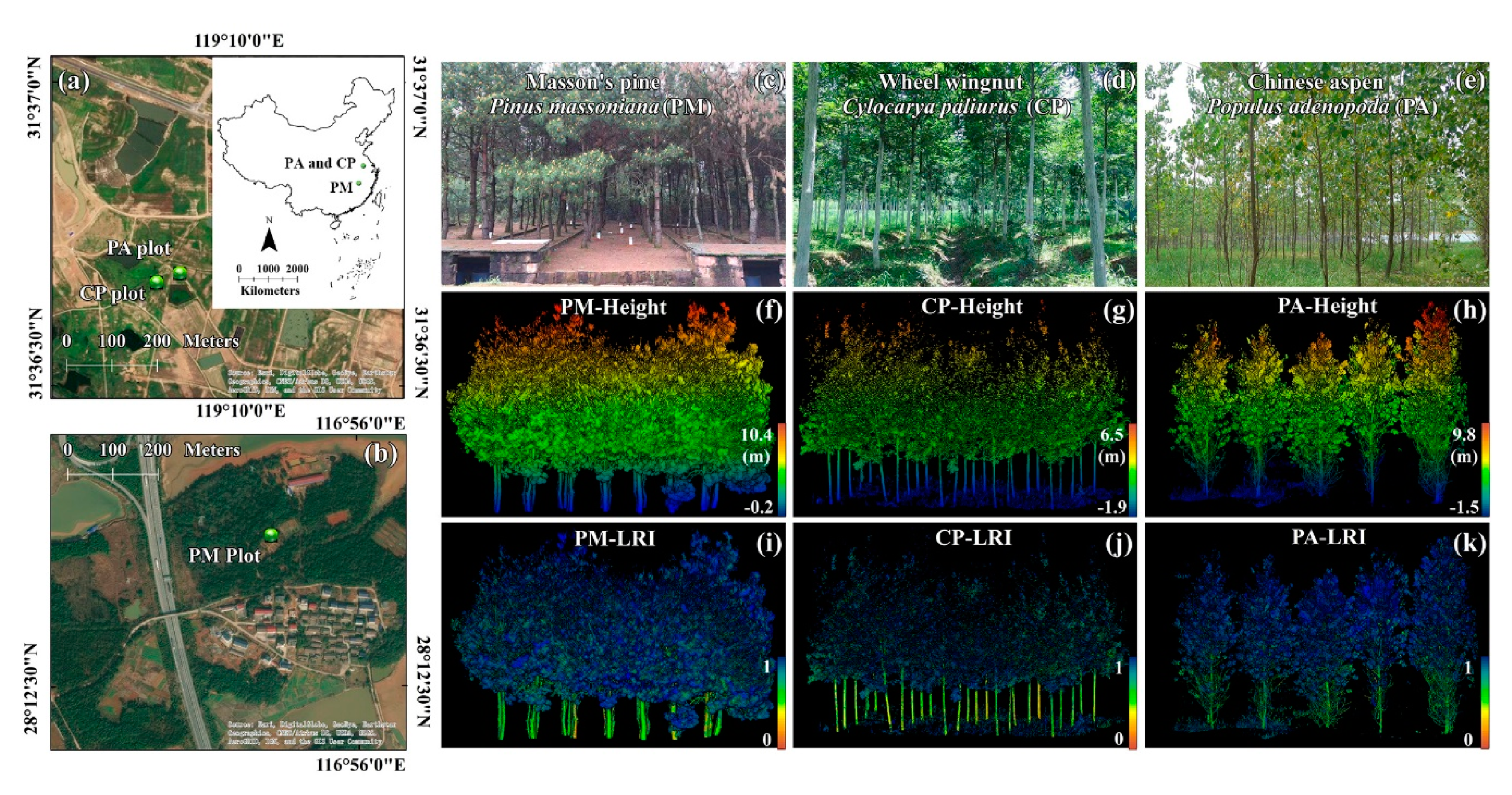
The study site comprises three human-planted plots with homogeneous tree species (Figure 1). We set up two broadleaf plots in the Baima research and experimental forest site in Nanjing (31°36′51″ N, 119°11′8″ E), Jiangsu province, China. The topography of the Baima site is relatively flat with shrubs and grasses, and the mean annual precipitation and temperature are 979 mm and 15.9 °C, respectively. The tree species grown in two plots are the Wheel wingnuts (Cyclocarya paliurus, CP) and Chinese aspens (Populus adenopoda, PA), respectively. The mean slope of the CP and PA plots are lower than 5°.

The coniferous plot with the tree species of Masson’s Pine (Pinus massoniana, PM) is in the red soil ecological experimental station of the Institute of Soil Science, Chinese Academy of Sciences (28°12′21″ N, 116°55′42″ E) in Yintan, Jiangxi province, China. The slope of the PM plot is 8° with a few grasses. The local mean annual precipitation and temperature are 1795 mm and 17.6 °C, respectively.

The canopy structure features of the three plots are different. Trees grown in the PA plot always had lateral branches attached to the middle and lower parts of their trunks. However, there were few lateral branches attached to the middle and lower parts of stems in the other two plots. More detailed characteristics of the three plots can be found in

Table 1. Summary statistics of the three plots. The DBH means the diameter at breast height, which was measured at 1.3 m upper on the ground. The std means the standard deviation of data.

Plots	Dimensions (m2)	Number of Trees	Height (m)		DBH (m)		Tree Age (Years)	Canopy Cover (%)
			mean	std	mean	std
PA	15×15	22	10.25	1.81	0.09	0.03	8	57
CP	15×15	25	6.84	0.27	0.08	0.01	7	84
PM	10×10	54	9.72	0.74	0.11	0.02	15	72

.

2.2. TLS Data

We collected discrete point cloud data using the Leica HDS 3000 TLS (Leica Geosystems AG, Heerbrugg, Switzerland) for the PA, CP, and PM plots on 26 July 2017, 21 July 2019, and 8 April 2019, respectively. The laser scanner worked at a height of 1.5 m above the ground with the 532 nm wavelength and a predefined angular resolution of 0.005 m at 10 m. The largest scan range of the TLS instrument was set as 20 m during the data collection.

In each plot, we set up one center and four corner scan locations to obtain five comprehensive field-of-view (i.e., horizontal: 0° to 360°; vertical: −45° to 90°) TLS scan. Three black-and-white targets were also set up at a height of 1.8 m to assist the multi-station data registration process. All point cloud data from five different locations were registered into a comprehensive TLS dataset for each plot using the Cyclone 9.0 software [40] with the registration error of less than 6 mm. Moreover, we normalized the pointwise LRI values from 0 to 1. Once the comprehensive TLS data of three plots were obtained, we filtered out the ground points using the Cloth Simulation Filter (CSF) tool [41] embedded in Cloud Compare (http://cloudcompare.org) software and manually removed the points of tripods and other objects except for points of trees and shrubs. To verify the robustness of the FWCNN model to data with diverse point density, we subsampled the PM and CP data. The average point density was: 552 points/unit for PA data, 68 points/unit for CP data, and 171 points/unit for PM data. Here, one unit means a sphere searching unit. The data subsampling tool embedded in the Cloud Compare software could help us to subsample the original TLS data.

In addition, we manually selected the foliage and woody points from the original TLS data based on the visual inspection. Two types of test points were manually labeled: 0 being foliage test points and 1 being woody test points. They were saved as the test point sets to evaluate the final classification results of the FWCNN model.

2.3. A CNN-Based Foliage and Woody Separation Model (FWCNN)

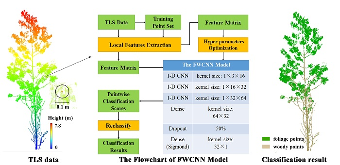
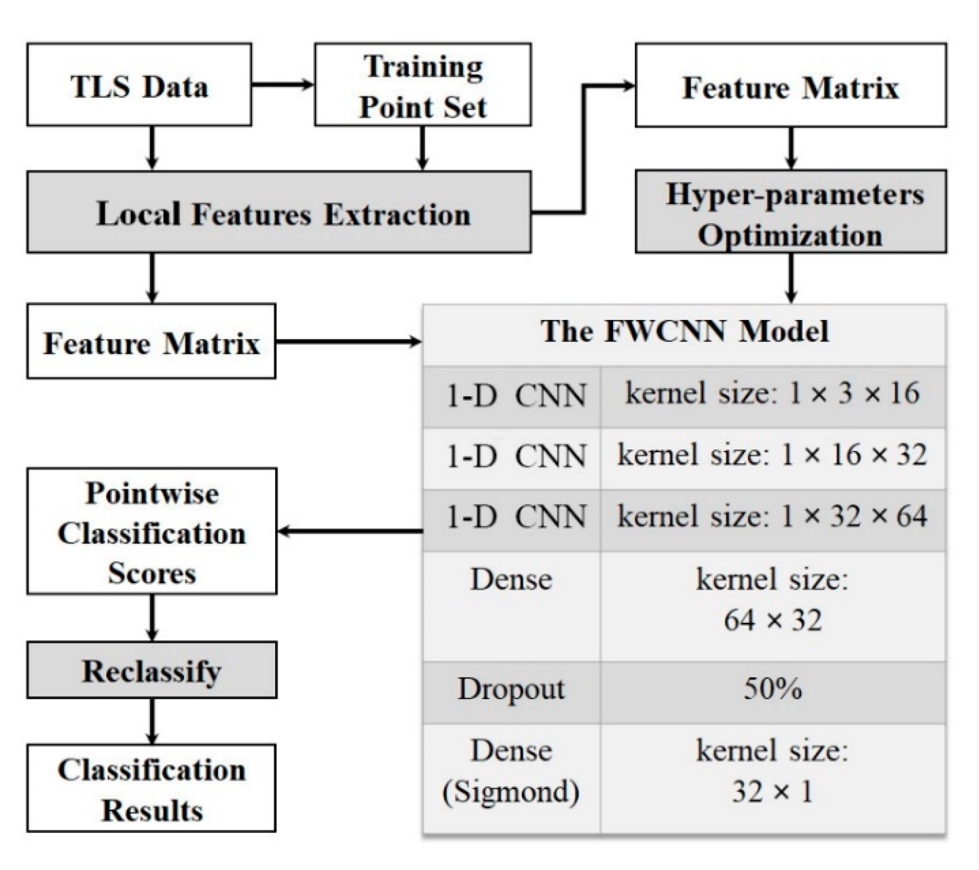
We propose a CNN-based foliage and woody separation (FWCNN) model in this study. The major steps are as follows: (1) we selected the training point sets from the original TLS data and computed the local features based on the geometrical and LRI information. (2) The hyper-parameter sets (i.e., learning rate, batch size, and validation split rate) of the FWCNN model were objectively determined and optimized. (3) The final classification results of foliage and woody components in forest TLS data were achieved based on the optimized FWCNN model. In addition, we quantitatively assessed the classification accuracy of the FWCNN-based approach in three forest stands including two broadleaved plots and one coniferous plot. The flowchart and architecture of the FWCNN model are shown in Figure 2.

2.3.1. The Architecture of FWCNN Model

To classify the TLS data, we modified the architecture of existing PointNet model [33] as follows: (1) Instead of only the spatial coordinates of discrete points, we input a feature matrix into the FWCNN model with three parameters including the morphological detection coefficient (MDC), the LRI values of each point and the averaged LRI values of local point sets within a certain sphere searching region around each point. (2) For the new proposed FWCNN model, we changed the CNN layers from 2-D to 1-D as we characterized the feature of each point based on a row matrix with three elements (MDC, the pointwise LRI and local mean LRI values) rather than the multiple 3-D coordinates of its local nearby points. (3) We removed the pooling layer to avoid learning invalid feature during the model training process. Moreover, we reset a smaller kernel size in each 1-D CNN layer than those in the PointNet model and removed a Dropout layer to improve the running efficiency of the FWCNN model. (4) In addition, we added the RMSprop optimizer [42] and binary cross-entropy function [39] to reduce the swing amplitude of loss function and assess the loss and validation loss rate in every epoch during the model training process.

By doing so, we obtained the final classification results based on the classification scores analyzed by the Sigmoid function in the last dense layer. We implemented the FWCNN model in Python 3.5 language programming environment based on the open-source software package Keras 2.2 [43].

2.3.2. Training Point Sets Selection

After removing the ground points, we divided each TLS data into multiple voxels with a fixed distance interval (D) based on their horizontal projection area. Without subdividing the point cloud data in the vertical direction, the height of one voxel equals the height difference of points inside it. In each voxel, the highest and lowest points were identified as H_max and H_min points. Then, we extracted points whose heights ranging from H_max m to (H_max − 0.5) m and from (H_min + 1) m to (H_min + 1.5) m as the candidate foliage and woody training sample points, respectively. The recommended value of D should be larger than the average range between neighbor stems to ensure that each voxel can contain stem points for choosing woody sample points (D was set as 3 m in this research). Then, we manually double-checked the selection results and removed the misidentified training sample points. The selected foliage and woody sample points were labeled as 0 and 1 in the training point sets (0 = foliage and 1 = woody training points), respectively. To evaluate the classification accuracy, we removed the intersection between the training and test point sets for each TLS dataset.

2.3.3. Point Feature Extraction

We extracted three different features of each point by combing the local geometrical and LRI information in TLS data as follows: (1) Morphological detection coefficient (MDC)—a geometrical feature to represent the 3-D distribution pattern of a local point set ${\mathrm{P}=\{\mathrm{p}}_{\mathrm{i}}{(\mathrm{x}}_{\mathrm{i}}{,\mathrm{y}}_{\mathrm{i}}{,\mathrm{z}}_{\mathrm{i}}),\mathrm{i}=1,2,\cdots ,\mathrm{n}\}$ that can be computed as:

$$\mathrm{MDC}=\frac{1}{{1+\mathrm{e}}^{\left(\mathsf{\lambda }\mathrm{a}-\mathsf{\lambda }\mathrm{b}\right)}\cdot {\mathrm{e}}^{\left(\mathsf{\lambda }\mathrm{c}-\mathsf{\lambda }\mathrm{b}\right)}},$$

(1)

where λ_a, λ_b, and λ_c (${\mathsf{\lambda }}_{\mathrm{a}}\ge {\mathsf{\lambda }}_{\mathrm{b}}\ge {\mathsf{\lambda }}_{\mathrm{c}}$) are three non-negative eigenvalues of the covariance matrix (C_cov) of P,

$${\mathrm{C}}_{\mathrm{cov}}=\frac{1}{\mathrm{n}}{\left(\stackrel{\rightharpoonup }{{\mathrm{p}}_{\mathrm{i}}}-\stackrel{\rightharpoonup }{\mathrm{p}}\right)}^{\mathrm{T}}\left(\stackrel{\rightharpoonup }{{\mathrm{p}}_{\mathrm{i}}}-\stackrel{\rightharpoonup }{\mathrm{p}}\right).$$

(2)

The row matrix $\stackrel{\rightharpoonup }{\mathrm{p}}$ is computed as:

$$\stackrel{\rightharpoonup }{\mathrm{p}}=\frac{1}{\mathrm{n}}{\displaystyle \sum _{\mathrm{i}=1}^{\mathrm{n}}{\left({\mathrm{x}}_{\mathrm{i}}{,\mathrm{y}}_{\mathrm{i}}{,\mathrm{z}}_{\mathrm{i}}\right)}^{\mathrm{T}}},$$

(3)

where T means the transposed matrix and $\stackrel{\rightharpoonup }{\mathrm{p}}$ is the row matrix of the mean coordinates for the n points in the given local point set P. The ordered eigenvalues of C_cov are the distribution morphological indices to represent the spatial distribution patterns of P [14]. When ${\mathsf{\lambda }}_{\mathrm{a}}{=\mathsf{\lambda }}_{\mathrm{b}}{=\mathsf{\lambda }}_{\mathrm{c}}$, the MDC equals 0.5 suggests that the n points in P are randomly distributed in 3-D space; If ${\mathsf{\lambda }}_{\mathrm{a}}{\text{> }\mathsf{\lambda }}_{\mathrm{b}}\approx {\mathsf{\lambda }}_{\mathrm{c}}$, the MDC is larger than 0.5 indicating a linear distribution pattern of points in P. The n points in P exhibit a surface distribution pattern when ${\mathsf{\lambda }}_{\mathrm{a}}\approx {\mathsf{\lambda }}_{\mathrm{b}}{\text{> }\mathsf{\lambda }}_{\mathrm{c}}$, and the MDC is smaller than 0.5. (2) Corrected LRI: We firstly sorted the LRI values of n points in the order from low to high within the given local point set P centered with point ${\mathrm{p}}_{\mathrm{c}}$. Then, we computed the local LRI reference range [LRI_min, LRI_max]:

$${\mathrm{LRI}}_{\min }{=\mathrm{LRI}}_{\mathrm{q}1}-1.5\cdot \mathrm{IQR},$$

(4)

$${\mathrm{LRI}}_{\max }{=\mathrm{LRI}}_{\mathrm{q}3}+1.5\cdot \mathrm{IQR},$$

(5)

where ${\mathrm{LRI}}_{\mathrm{q}1}$ means the lower (i.e., 25%) quartile of LRI values for n points, ${\mathrm{LRI}}_{\mathrm{q}3}$ means the upper (i.e., 75%) quartile of LRI values for n points, and IQR means the interquartile range of LRI values for n points [44]. The LRI value of ${\mathrm{p}}_{\mathrm{c}}$ will be kept if its LRI is within the local LRI reference range, otherwise, the LRI value of ${\mathrm{p}}_{\mathrm{c}}$ will be replaced by the median LRI of n points in P. (3) Mean LRI of local points: The mathematical mean LRI values of the n points in P was added as an additional attribute of the center point ${\mathrm{p}}_{\mathrm{c}}$. Three categories of features were normalized into the range from 0 to 1 to form a 3-D feature matrix and input into the FWCNN model. Before the FWCNN running stage, we computed the feature matrixes for the TLS dataset and training point set of each plot, respectively.

2.3.4. Hyper-Parameters Determination

We determined the values of batch size, learning rate, and validation split rate using the cross-validation method by the following steps: (1) We first randomly selected the initial values for batch size (B) and validation split rate (V) each ranging from 0 to 100% and learning rate (LR) to form a hyper-parameter set. The value of B means using B percentage of all training samples to form a batch to train the FWCNN model in every epoch, while the value of V indicates the V percentage of samples in one batch input into the FWCNN model to validate the classification accuracy after every epoch during the model training process [39]. In terms of the LR, we determined its tested range based on the method proposed by Smith [45]. (2) Then, we recorded the validation loss ratio (VLR) in each epoch and calculated the absolute difference values between n-th and (n-1)-th elements in VLR to form a data matrix (D_VLR). If the k-th element in D_VLR approached to 0, the (k-1)-th element in the corresponding VLR was chosen as a candidate convergence point (CON_p) for the validation loss function of a given hyper-parameter set. By doing so, a group of CON_p points was selected for a given validation loss function. (3) In the next step, we determined the convergence point of the given validation loss function. For a group of CON_p points, the first 3-number-continuous data values indicated the starting convergence point of the validation loss function. Hence, the first number of 3-number-continuous data would be determined as the convergence point (C). For example, for a group of candidate CON_p list {6, 9, 10, 17, 18, 19}, the subset {17, 18, 19} was the first 3-number-continuous data, within which the first number 17 would be determined as the convergence point of the validation loss function. (4) Finally, we used the following function to compute the contribution score (S) for the given hyper-parameter set:

$$\mathrm{S}=\{\begin{array}{ll}{(1-{\mathrm{L}}_{\mathrm{low}})}^{\mathrm{c}}& (\mathrm{E}\ge \mathrm{C}\ge \mathrm{E}/4\&{\mathrm{L}}_{\mathrm{low}}<1)\\ 0& (\mathrm{C}<\mathrm{E}/4)\\ -1& ({\mathrm{CON}}_{\mathrm{p}}=\left\{\right\})\\ -2& ({\mathrm{L}}_{\mathrm{low}}\ge 1)\end{array},$$

(6)

where L_low is the C-th element in VLR; E means the initial epoch times during the FWCNN model training stage (E was set as 20 in this research). The fitted FWCNN model using the given hyper-parameter set will be an over-fitting one if S = 0, while it will be an invalid model if S = −2. In the case of S = −1, it indicates that the validation loss function is not convergent by using the given hyper-parameter set (the CON_p is a null list), and the FWCNN model was under-fitting. Finally, all positive S were normalized into the range from 1 to 10 and saved as integers.

Besides, we optimized the epoch time of the model training process based on the mode of parameter C to improve the running efficiency of the FWCNN model. After running the FWCNN model using the optimized hyper-parameter set, we obtained the point-wise classification scores analyzed by the Sigmoid function. The pointwise classification scores were still needed to reclassify into two categories to denote foliage or woody points. We used the Natural Breaks method [46] embedded in the open-source Pysal package [47] to determine the reclassification threshold (RT). Finally, we denoted the points whose classification scores were higher than RT as the woody points and the rest points in the same TLS dataset as the foliage points.

2.4. Sensitivity Analysis

To evaluate the effects of searching radius to the final classification accuracy of the FWCNN model, we extracted the local features of each point in three TLS datasets using the searching radii changing from 0.03 m to 0.1 m with an increment of 0.01 m.

Moreover, we evaluated the effects of point density variations on the robustness of the FWCNN model. The point cloud data of each plot was subsampled into 7 ranks: from 552 points/unit to 79 points/unit for PA data, from 68 points/unit to 10 points/unit for CP data, and from 171 points/unit to 26 points/unit for PM data. Here, the unit means one sphere searching region with a fixed radius. Finally, we used the FWCNN model to classify subsampled TLS data of each plot and compared their classification accuracy using the original TLS data.

2.5. Accuracy Assessment

To evaluate the final classification accuracy, we calculated the overall classification accuracy (OA), the producer’s accuracy of foliage points (FPA), the producer’s accuracy of woody points (WPA) and the Kappa coefficient based on the following Equations (Equations (7)–(12)):

$$\mathrm{OA}=\frac{{\mathrm{V}}_{\mathrm{f}}{+\mathrm{V}}_{\mathrm{w}}}{{\mathrm{T}}_{\mathrm{f}}{+\mathrm{T}}_{\mathrm{w}}},$$

(7)

$$\mathrm{FPA}=\frac{{\mathrm{V}}_{\mathrm{f}}}{{\mathrm{T}}_{\mathrm{f}}},$$

(8)

$$\mathrm{WPA}=\frac{{\mathrm{V}}_{\mathrm{w}}}{{\mathrm{T}}_{\mathrm{w}}},$$

(9)

where V_f and V_w are the numbers of true classified foliage and woody points in one test point set; T_f and T_w are the numbers of foliage and woody points in the same test point set. The Kappa coefficient is computed as:

$$\mathrm{Kappa}=\frac{{\mathrm{P}}_0{-\mathrm{P}}_{\mathrm{c}}}{{1-\mathrm{P}}_{\mathrm{c}}},$$

(10)

$${\mathrm{P}}_0=\frac{{\displaystyle \sum _{\mathrm{i}=1}^{\mathrm{r}}{\mathrm{X}}_{\mathrm{ii}}}}{\mathrm{N}},$$

(11)

$${\mathrm{P}}_{\mathrm{c}}=\frac{{\displaystyle \sum _{\mathrm{i}=1}^{\mathrm{r}}\left({\mathrm{X}}_{\mathrm{i}+}\cdot {\mathrm{X}}_{+\mathrm{i}}\right)}}{{\mathrm{N}}^2},$$

(12)

where P₀ means the relative observed agreement among N samples in error matrices with r rows, which is equal to the ratio of the sum of the correct identification samples of all samples belonging to the same type; the P_c is the hypothetical probability of chance agreement; X_i+ and X_+i are the row probabilities and the column probabilities, respectively.

To assess the contribution of combining the LRI and geometrical information in distinguishing TLS data, we used the LeWoS model [32] and LWCLF model [15], which are only based on geometrical features, to classify the TLS datasets, and evaluated their classification accuracy for foliage and woody components. Additionally, we compared the FWCNN-based results with those obtained using the Random Forest (RF) algorithm [48], Gaussian Mixed Model (GMM) [30], and Support Vector Machine (SVM) algorithm [49] in terms of classification accuracy and running efficiency. These four classifiers used the same features extracted from TLS data to classify woody and foliage components. Moreover, we evaluated the effects of LRI correction on the final classification results. The McNemar’s test [11,50] was used to evaluate the statistical significance between the results obtained using the FWCNN model and those obtained using another classifier (SVM, RF, GMM, LeWoS, or LWCLF), and using original and post-corrected LRI information. The codes of the LeWoS model and LWCLF model can be downloaded from https://github.com/dwang520/LeWoS.git and https://github.com/sruthimoorthy/leaf_wood_clf.git, respectively. The other three classifiers (RF, GMM, and SVM) were programmed using Scikit-Learn 0.21.3 [51]. All classifiers were run on the same computer system with a 3.40GHz Intel Core i7-3770 processor with 16 GB memory.

3. Results

3.1. Extracted Point Features

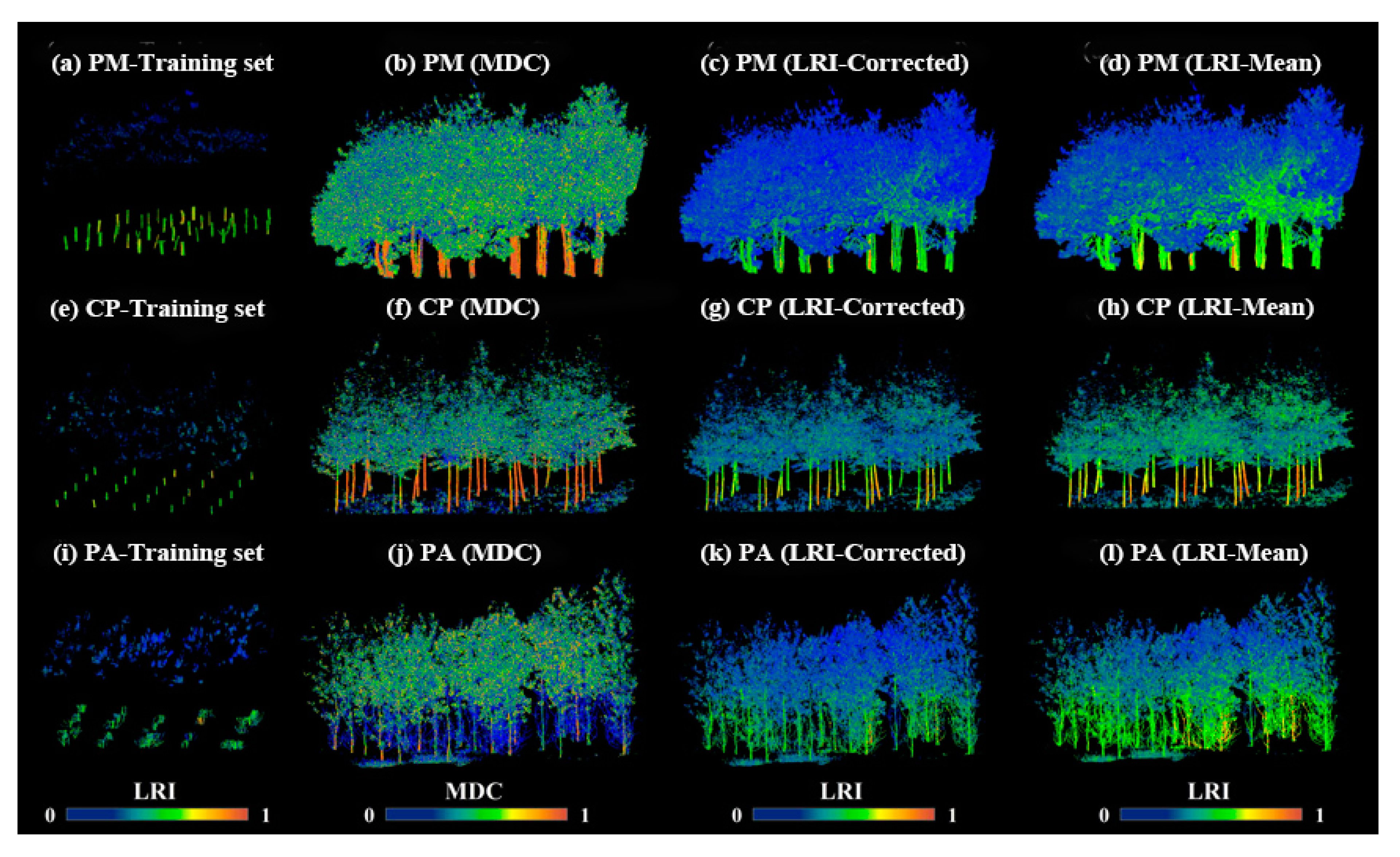
To train the FWCNN model, we chose 490,633 points (6.81% of all points in TLS dataset) from the PA data, 136,829 points (7.52% of all points in TLS dataset) from the CP data, and 620,057 points (2.82% of all points in TLS dataset) from the PM data as the training point sets. Meanwhile, we obtained the optimal searching radius as 0.05 m to extract the point features based on the methods described in Section 2.4. After point-wise extraction of the local MDC and the two LRI-related features from the comprehensive TLS dataset and training point sets, we obtained two types of 3-D feature matrices to run the FWCNN model. The training point sets selected from each TLS dataset and the three matrices extracted from each TLS dataset, including the MDC, the corrected LRI information of each point (LRI-Corrected), and the pointwise local mean LRI (LRI-Mean), are shown in Figure 3.

3.2. Determination of the Optimal Hyper-Parameter Set

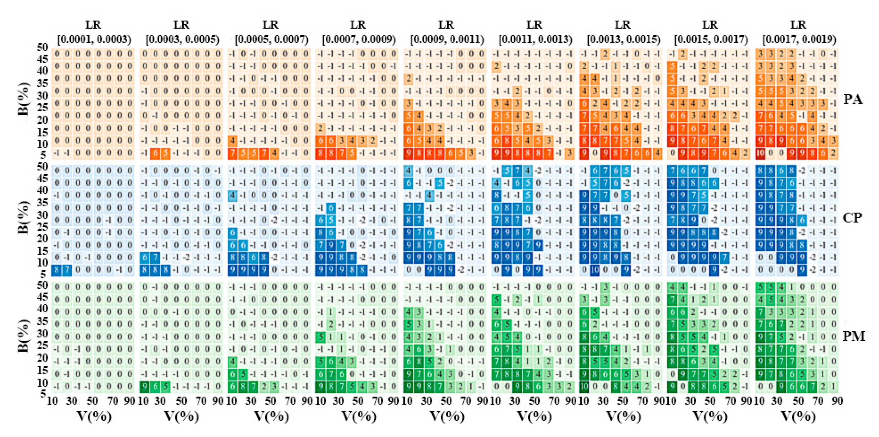
We randomly selected the learning rate within (0.0001, 0.0019), the batch size within (5%, 50%) of the number of all training samples, and the validation split rate within the range (10%, 90%) to form test hyper-parameter sets. In total, 3260 hyper-parameter sets (for CP data: 1074 sets, for PA data: 1157 sets, for PM data: 1029 sets) were selected and evaluated based on the method described in Section 2.3.4. The contribution scores of all tested hyper-parameter sets are shown in Figure 4. In Figure 4, the number in each grid is the average contribution score of the tested hyper-parameter sets which were randomly chosen within the related range of the given grid.

Based on a comparison of these scores, the learning rate was set as 0.0015, the batch size as 10% of the number of training samples in one batch, and the validation split rate was 20% in the FWCNN model. If the validation split rate was set as <50% and over 50% of samples in one batch were used to train the FWCNN model, the contribution scores of the tested hyper-parameter sets were more likely to be greater than 7. Meanwhile, if the validation split rate was set as ≥ 50% and over 50% of samples in one batch were used to train the FWCNN model, the scores of the related hyper-parameter sets were almost all equal to −1 when processing the CP and PA data. For the tested hyper-parameter sets with a learning rate ≥ 0.0009, setting the validation split rate to above 50% caused model under-fitting. However, for PM data, setting the validation split rate ≥ 50% caused model instability, and the scores of the related tested hyper-parameter sets changed between 0 and −1. Thus, the optimal validation split rate should be set lower than 50% when using the FWCNN model to classify three TLS datasets.

We tested various batch sizes less than or equal to 50% of training samples in each TLS dataset to train the FWCNN model. The scores of the hyper-parameter sets were almost all lower than 1 when setting the learning rate at < 0.0009 and the batch size in one epoch at > 20% of all training samples to classify the PA and PM data. Keeping the learning rate constant and only increasing the batch size could not significantly raise the scores of the tested hyper-parameter sets, but reduced the model training efficiency for the PA and PM data. For the hyper-parameter sets with a learning rate ≥ 0.0009, setting the batch size to ≤20% was more likely to obtain scores ≥ 7. Thus, using batch sizes of ≤ 20% of training samples selected from the TLS dataset was suitable to train the FWCNN model.

The learning rate was tested within [0.0001, 0.0019) in different hyper-parameter sets. As shown in Figure 4, over half of the hyper-parameter sets had scores < 1 when using learning rates < 0.0011. This means that using learning rates < 0.0011 was more likely to result in over-fitting (i.e., scores = 0), under-fitting (i.e., scores = −1), or an ineffective model (i.e., scores = −2) during training. For a hyper-parameter set with a batch size of ≤ 20% and a validation split rate of < 50%, using learning rates within [0.0011, 0.0017) was more likely to obtain scores of ≥ 7. When setting the batch size to 10% and the validation split rate to 20%, the scores of the tested hyper-parameter sets with a learning rate within [0.0011, 0.0017) were similar. Thus, slightly changing the learning rate did not seriously affect the classification accuracy of the FWCNN model.

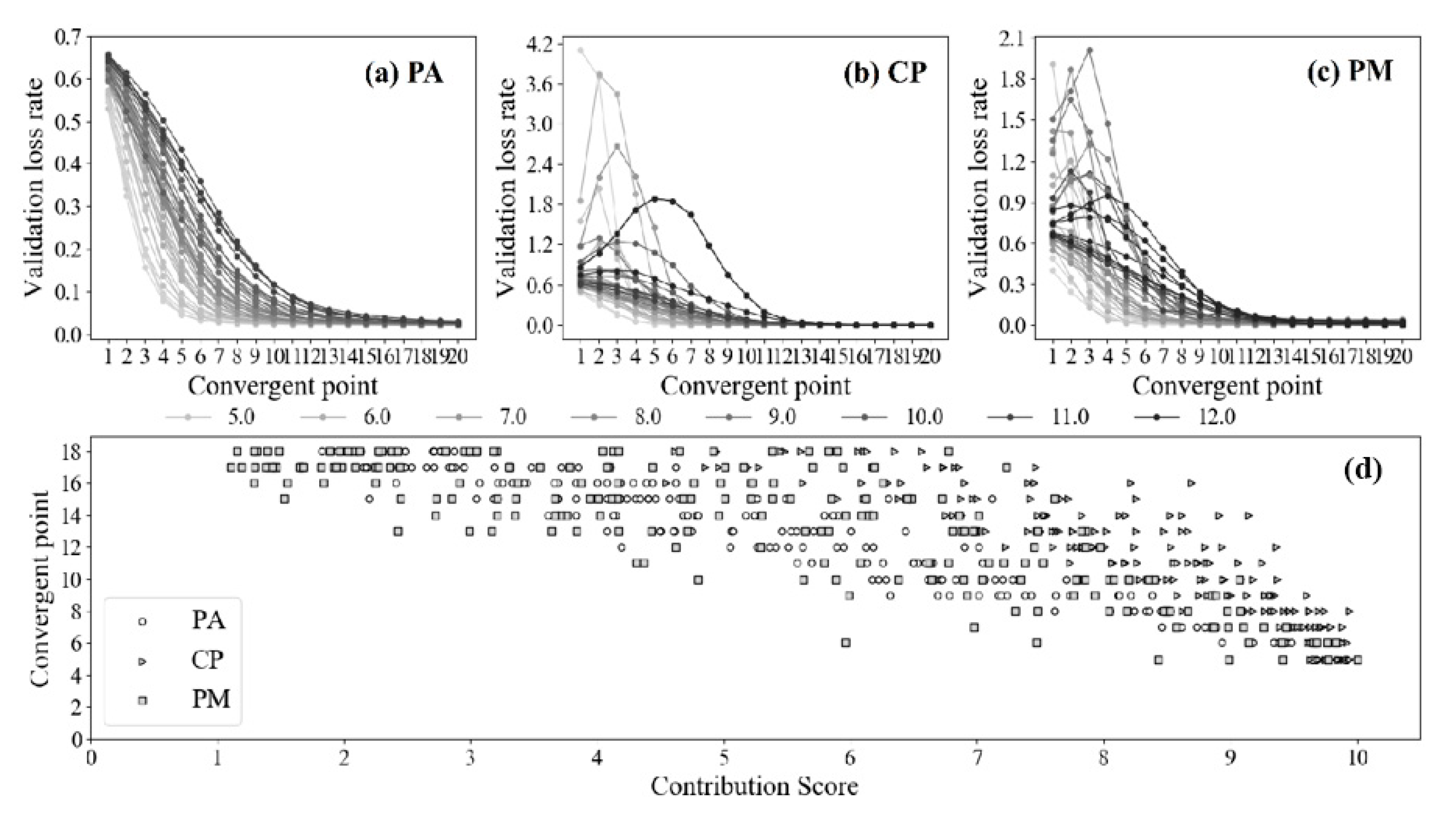
Figure 5a–c show the validation loss rate of the FWCNN model during the model training process within 20 epochs (a total of 150 tested hyper-parameter sets, 50 sets for each TLS dataset). From these three subfigures, it is evident that the convergence points of the validation loss functions could be accurately detected, where the validation loss functions of high-scoring sets (score >7) always converge before 10 epochs during the model training process (Figure 5d). In order to increase the training efficiency of the FWCNN model, we reset the epoch time to 10.

3.3. Point-Wise Classification Results

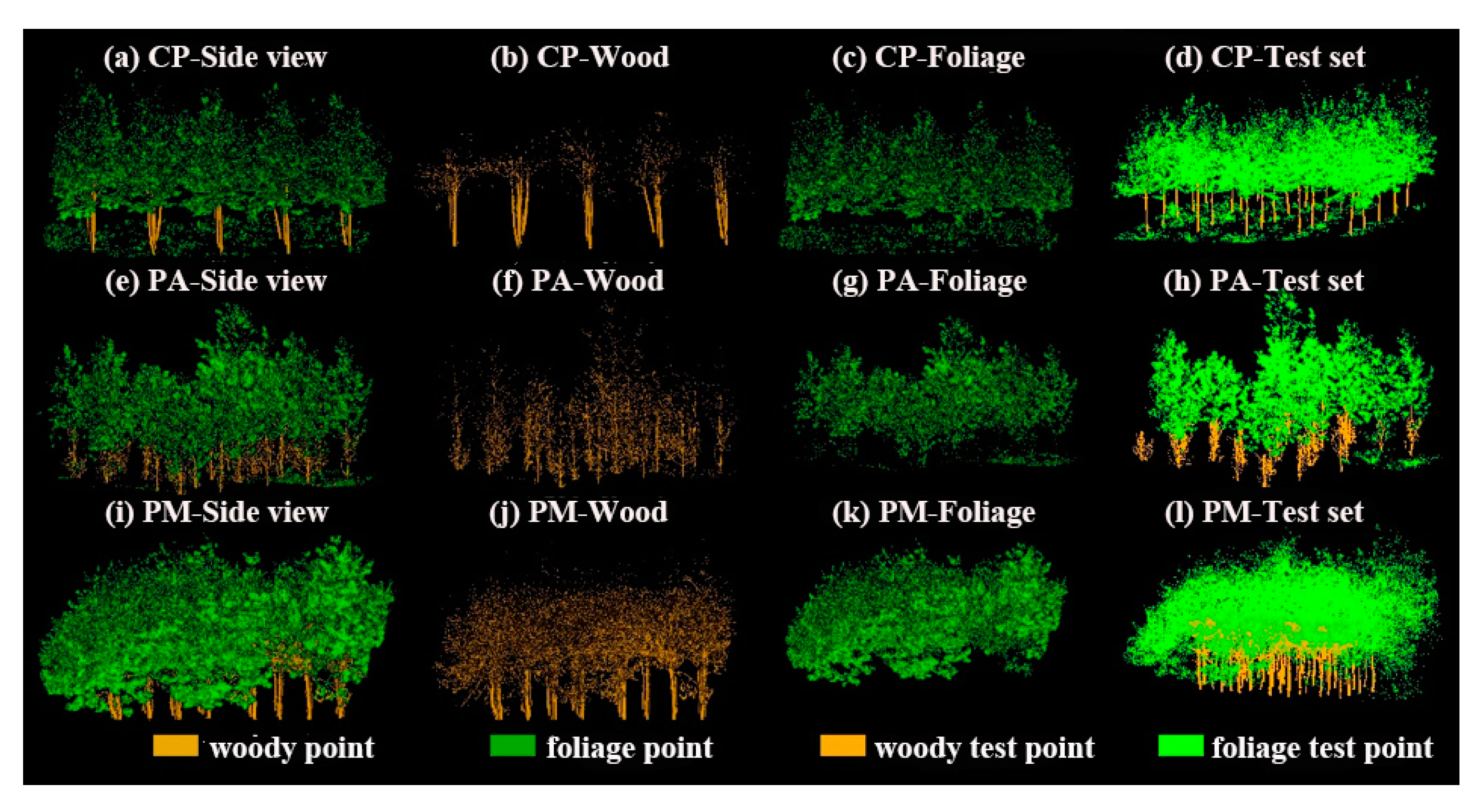
The OA of using the FWCNN model was 98.64% for PA data, 96.20% for CP data, and 94.98% for PM data (all with Kappa ≥ 0.89 for LRI-corrected data). The classification results of three TLS datasets are shown in Figure 6. To evaluate the classification accuracy, we manually selected 1475939 points (826,062 woody points and 649,877 foliage points) from PA data, 913,081 points (265,594 woody points and 647,487 foliage points) from CP data, and 937,688 points (567,889 woody points and 369,799 foliage points) from PM data (shown in Figure 6) as the test point sets. The details about time cost, the producers’ accuracy of foliage (FPA) or woody (WPA) points from three TLS datasets, and the reclassification threshold (RT) of FWCNN results (classification scores) are shown in

Table 2. Comparing the classification accuracy of using six types of classifiers (FWCNN, GMM, RF, SVM, LeWoS, and LWCLF) to separate woody and foliage points from (original and LRI-corrected) TLS data. Within these classifiers, the LeWoS and LWCLF models only used the geometric-based features to classify woody and foliage components from TLS data. The RT means the threshold to reclassify the pointwise classification scores analyzed by the FWCNN model. The data in the time column show the time consumption of running four types of classifiers apart from the feature extraction process. We did not list the time cost of two geometric-based models owing to their feature extraction methods were different from the other four classifiers. The F-T and W-T mean the number of foliage and woody points that were correctly classified within the test sets. The OA means the overall classification accuracy. The FPA and WPA mean the producer’s accuracy of foliage and woody points in the classification results, respectively.

TLS Data	LRI	Classifiers	RT	Time (s)	W-T (Point#)	F-T (Point#)	OA (%)	WPA (%)	FPA (%)	Kappa
PA	corrected	FWCNN	0.49	137	816,066	639,869	98.64	98.79	98.46	0.97
		GMM	-	33	808,562	631,871	97.59	97.88	97.23	0.95
		RF	-	32	813,432	622,106	97.26	98.47	95.73	0.94
		SVM	-	754	808,353	632,377	97.61	97.86	97.31	0.95
	original	FWCNN	0.49	135	813,562	637,298	98.30	98.49	98.06	0.97
		GMM	-	31	796,810	629,770	96.66	96.46	96.91	0.93
		RF	-	29	808,417	616,506	96.54	97.86	94.87	0.93
		SVM	-	671	803,259	627,360	96.93	97.24	96.54	0.94
		LeWoS	-	-	685,618	583,042	85.96	82.99	89.72	0.72
		LWCLF	-	-	778,704	596,518	93.18	94.27	91.79	0.86
CP	corrected	FWCNN	0.5	54	239,251	639,109	96.20	90.08	98.71	0.91
		GMM	-	19	245,037	624,667	95.25	92.26	96.48	0.89
		RF	-	25	249,884	615,426	94.77	94.08	95.05	0.88
		SVM	-	392	244,075	612,920	93.86	91.90	94.66	0.85
	original	FWCNN	0.49	53	250,730	617,133	95.05	94.40	95.31	0.88
		GMM	-	24	234,537	614,167	92.95	88.31	94.85	0.83
		RF	-	28	244,619	610,533	93.66	92.10	94.29	0.85
		SVM	-	457	244,012	612,913	93.85	91.87	94.66	0.85
		LeWoS	-	-	242,131	515,749	83.00	91.16	79.65	0.63
		LWCLF	-	-	260,947	514,708	84.95	98.25	79.49	0.68
PM	corrected	FWCNN	0.53	156	557,925	332,661	94.98	98.25	89.96	0.89
		GMM	-	42	474,793	337,737	86.65	83.61	91.33	0.73
		RF	-	61	555,355	309,153	92.20	97.79	83.60	0.83
		SVM	-	712	550,389	315,621	92.36	96.92	85.35	0.84
	original	FWCNN	0.51	152	555,381	320,991	93.46	97.80	86.80	0.86
		GMM	-	34	457,293	320,237	82.92	80.53	86.60	0.65
		RF	-	58	550,377	303,886	91.10	96.92	82.18	0.81
		SVM	-	875	545,353	310,619	91.29	96.03	84.00	0.81
		LeWoS	-	-	438,141	272,671	75.80	77.15	73.73	0.50
		LWCLF	-	-	405,122	289,273	74.05	71.34	78.22	0.48

. Meanwhile, the classification accuracy of using the FWCNN model to separate the LRI-corrected data was compared with those of five other classifiers for the separation of woody and foliage points from TLS data and using the original TLS data without LRI correction. By the McNemar’s test, the differences between using the FWCNN model and another classifier (GMM, RF, SVM, LeWoS, or LWCLF), and using original and post-corrected LRI information, were statistically significant with p < 0.05.

3.4. The Results of Sensitivity Analysis

In this research, the optimal searching radius to extract features from three TLS datasets was determined as 0.05 m. As shown in Figure 7, the OA varied markedly when using different searching radii to extract features from the PM data, however was steady when classifying the PA data. For all tested TLS data, the highest OA were obtained when using a searching radius of 0.05 m to extract features (PM data: 94.98%, Kappa = 0.89; CP data: 96.20%, Kappa = 0.91; PA data: 98.64%, Kappa = 0.97). When setting the searching radius > 0.05 m, the OAs for the PA and PM data decreased slightly compared to the OAs for a searching radius of 0.05 m (with Kappa > 0.80). Meanwhile, setting the searching radius < 0.04 m dramatically decreased the OA for PM data compared to the OA for a searching radius of 0.05 m. The WPAs of the PM data were over 90% when using different searching radii, while its FPAs were lower than 90%. More foliage points were misclassified as woody points in PM data when the searching radius was set > 0.06 m compared to when the radius was set at 0.05 m. The FPAs for the two broadleaf (PA and CP) point cloud data were similar (> 95%) when the searching radius was set < 0.09 m. However, more than 10% of woody test points were misclassified as foliage points in the CP data when the searching radius was set < 0.09 m.

To evaluate the effect of point density on the classification accuracy, we subsampled the three TLS datasets into seven ranks (as shown in Figure 7d–f), and distinguished foliage and woody points from data with different point densities using the FWCNN model. It was found that, for the two broadleaf TLS datasets, the OAs gradually decreased with decreasing point density; however, the OA was still similar to that obtained using the original data after halving the point density. For the PA data, the classification accuracy indices were more sensitive to the variable point density than for the CP data. Reducing the point density led to a reduction in the WPA of PA data from over 97% to 88%.

4. Discussion

4.1. Effects of Hyper-Parameter Selection

In this research, we modified the architecture of the PointNet model [33] to design the FWCNN model. Meanwhile, we paid more attention to quantitatively evaluate and objectively select three hyper-parameters used in the FWCNN model, which greatly affect the model performance. Previous studies describing CNN-based models rarely mentioned the methods used to set hyper-parameters objectively.

The batch size and validation split rate control the training sample size in each epoch. Setting an appropriate number of samples in each epoch during the model training process is preferable to balance the training efficiency and avoid memory overflow [52]. In this research, we set the batch size as 10% of the number of training samples selected from each TLS dataset, instead of using a fixed number of samples in each epoch during the model training process, since this is more suitable for processing TLS data with variable point density. Generally, the learning rate is more important than the sample size for training a deep learning model [38]. Setting an overly large learning rate and using an overly small number of training samples would cause model over-fitting. If there are a large number of samples in each training epoch, it is necessary to increase the learning rate to prevent training model under-fitting. Here, we recommended using the method proposed by Smith [45] to determine the optimal learning rate for deep learning models.

Some researches set hyper-parameters using a rule-of-thumb [29,33,53]. The use of reliable expert knowledge can increase the efficiency of hyper-parameter optimization for deep learning models. However, for users without any prior experience of training a CNN-based model, using the score evaluation method mentioned in Section 2.3.4 in combination with the cross-validation test is a feasible way to choose the optimal hyper-parameter set. When using the FWCNN model to classify other TLS datasets, users can use the optimal hyper-parameter set selected by us in preference.

4.2. Factors Affecting Classification Accuracy

4.2.1. Searching Radius

Setting the suitable searching radius is a key step before training the FWCNN model as choosing the optimal radius increases the classification accuracy. Using an excessively small searching radius cannot adequately capture the geometrical features of local points. For example, for a searching radius of 0.02 m, the MDC values of local points covered on thick branches might similar to the MDC values of local points covered on the single broadleaves. Meanwhile, setting too small a search radius will reduce the number of points in one search unit, which is not beneficial to correct the LRI information. Some previous studies found that setting the searching radius near 0.45 m was suitable for extracting the local geometrical features of point cloud data [9,14,54]. However, the LRI information of local points may reflect from both woody and foliage components when setting the 0.45-m searching radius. In this condition, the local LRI-related features cannot be used to denote woody or foliage points. Thus, in this work, we set the searching radius as 0.05 m to extract the local features in discrete TLS data.

4.2.2. Point Density

The point density is another factor that can affect the classification results in similar researches [9,10,15]. However, the results of this study verified that the classification results obtained using the FWCNN model are insensitive to the point density variation of tested TLS datasets. During this test, the searching radius was maintained at 0.05 m to extract features from subsampled TLS data. Then, we used the intersection between the original test point sets and the subsampled TLS data as the test point sets for the subsampled TLS data in order to evaluate the OA, FPA, WPA, and Kappa coefficient for all classification results. We found the classification accuracy indices of PA data were more sensitive to the variable point density. A possible reason for this may be that the local distribution of points from lateral branches attached to the trunks of trees in the PA plot changed after data subsampling. Furthermore, it was found that the OA and FPA of PM data increased slightly when using a subsampled point cloud data. A possible reason for this may be that the redundant points caused by laser scatter near the needle clusters within the canopy of the PM plot were partly filtered out after data subsampling. For a broadleaf plot with interlacing branches and twigs, better classification results were obtained when using TLS data with a higher point density to classify foliage and woody points.

4.2.3. LRI Correction

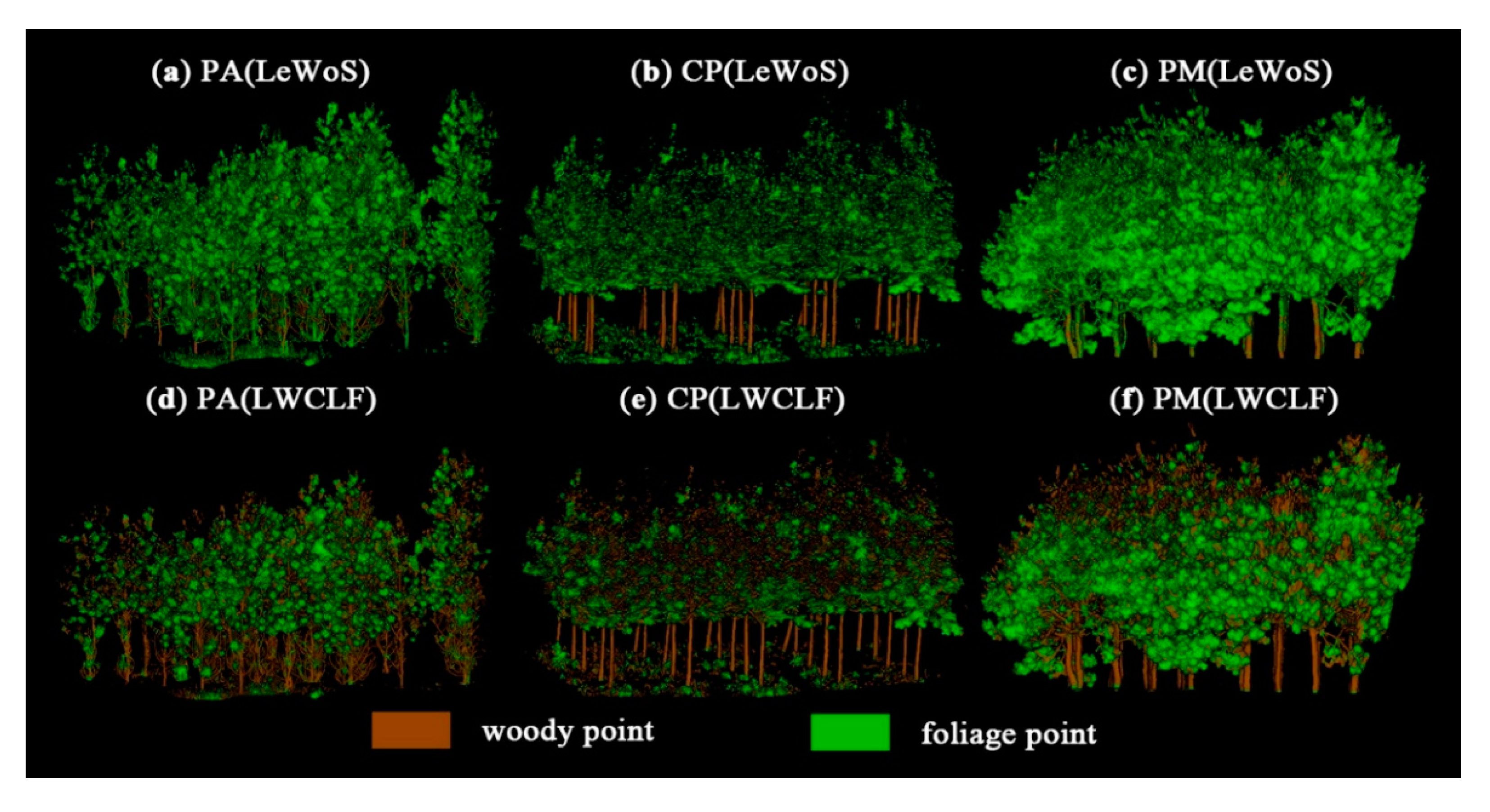
As shown in Figure 3, the MDC values of points from lateral branches of trees are different from the MDC values of points covered on the trunks in the PA plot. However, over 20% of foliage test points from broadleaves and needle clusters in the CP and PM plots were misclassified as woody points in the classification results of the LeWoS and LWCLF models (as shown in Table 2). In Figure 8, these two geometric-based models always concern local point sets with a linear distribution trend as the woody point sets and point sets with random and patch distribution trends as the foliage points. If we only based on the geometrical features to classify foliage and woody points, the points from interlacing branches were always misclassified as foliage points. Besides, the points from broadleaves and needle clusters with near-vertical leaf inclination angles were always classified as woody materials. Previous studies obtained similar results when using geometric-based classification models [10,32]. When combining the LRI- and geometric-based features to separate the foliage–woody components from TLS data, the OA increased at least 5%. Thus, combining pointwise LRI information with local geometrical features could help to classify woody and foliage materials in TLS data collected from forests with complex structural features, especially the coniferous forests.

Compared with using the original TLS data, we found that the LRI correction method used in this study (see Section 2.3.3) increased the classification accuracy of the four classifiers using the LRI-related features. In the FWCNN results, the OAs of all tested TLS datasets increased after the LRI correction, especially that of the CP data (whose OA increased from 95.05% to 96.20%) and the PM data (whose OA increased from 93.46% to 94.98%). In principle, the foliage or woody points in the point cloud data of one tree crown should have similar LRI values to the laser pulse. However, the variability of sensor-related parameters and environmental factors during the multi-station data collection may introduce noise to the LRI information—for example, the variable distance between the laser scanner and targets, the variable incidence angle of laser return signals, the variation in weather conditions (wind and fog), and the occlusion on the transmission path of laser pulse [20]. The local points within a spherical searching unit may be from multiple scan stations after data registration, while the scan angle and laser transmission range are not pointwise recorded in discrete TLS data. Meanwhile, users cannot know the specific method used to interpret the pointwise LRI information recorded in TLS data [16]. When using the same laser scanner to collect point cloud data, we infer that the interpretation method of laser return singles had little effect on the pointwise LRI information collected from multiple scan stations. It is difficult to precisely calibrate the LRI information of a multi-station TLS data.

The LRI correction method used in this research does not require any prior knowledge about scanner parameters or field data about targets’ reflectance. However, the relationship between the corrected LRI and the real backscatter reflectance of targets is still unknown after correcting the LRI information in TLS data. To further verify the proposed LRI correction method, in the future, we plan to conduct a field survey to evaluate the correlation between the backscatter reflectance of targets to laser pulse and the post-corrected LRI values of points from the same targets.

4.2.4. Reclassify the Classification Scores

The classification results of the FWCNN model were still needed to be reclassified as two types to denote woody and foliage points, because they were classification scores within [0, 1]. We found setting the reclassification thresholds (RTs) as 0.5 was unbeneficial to reclassify the FWCNN results. In

Table 3. The classification accuracy of the FWCNN model after setting the reclassification threshold (RT) as 0.5 or using the RT values determined by the Natural Breaking (NB) method. In this table, the F-T and W-T mean the number of foliage and woody points that were correctly classified within the test sets. The OA means the overall classification accuracy. The FPA and WPA mean the producer’s accuracy of foliage and woody points in the classification results, respectively.

TLS Data	RT	W-T (Point#)	F-T (Point#)	OA (%)	WPA (%)	FPA (%)	Kappa
PA	0.5	814,229	635,852	98.25	98.57	97.84	0.96
	0.49	816,066	639,869	98.64	98.79	98.46	0.97
PM	0.5	544,513	320,606	92.26	95.88	86.70	0.84
	0.53	557,925	332,661	94.98	98.25	89.96	0.89

, the RTs of PM and PA data analyzed by the Natural Breaks (NB) method were not equal to 0.5. We tested to set the RT as 0.5 to reclassify the pointwise classification scores of PM and PA data. The results are shown in Table 3. The CP data were not included in Table 3, as its RT value was determined as 0.5 by the NB method. For the PA data, the OAs were similar when setting the RT as 0.5 or 0.49 (analyzed by the NB method). However, the OA fell from 94.98% to 92.26% for PM data when we set the RT as 0.5. Meanwhile, its FPA and WPA decreased from 89.96% to 86.70% and from 98.25% to 95.88%, respectively. By the McNemar’s test, the p values were all lower than 0.05, which verified that the differences between the classification results after setting diverse RT were statistically significant.

4.3. Comparisons with Other Classifiers Using LRI Information

We compared the results of the FWCNN model with those of three other classifiers—namely RF, GMM, and SVM—for the separation of woody and foliage points from TLS data (both original and LRI-corrected). As shown in Table 2, the OA of the PM data was generally lower than the OAs of the two TLS datasets of broadleaved trees (the PA and CP data). It was found that the FWCNN model always obtained higher OA values than the other three classifiers, although its time cost was higher than those of the RF and GMM models. The SVM model obtained the second-highest OA for the PA and PM data. However, the time cost of the SVM model was over five times higher than those of the RF and GMM models, which was also found by [30,31]. Thus, the SVM model was not an effective method to classify foliage and woody points from high-density TLS data with large data volumes. The GMM model obtained higher OAs than the RF model for separating foliage and woody points from the PA and CP data, while the RF model obtained a higher OA than the GMM model for the PM data.

In the FWCNN results of PM data, over 10% of foliage points were misclassified as woody points (FPA = 89.96%, WPA = 98.25%). We infer that the main reason for this is that the point cloud data of needle clusters may show a random distribution (as shown in Figure 3b), similar to the local geometrical features of points covered on the interlacing twigs (as shown in Figure 3j). Meanwhile, it was found that the LRI values of points from withered needle clusters were significantly higher than those covered on fresh needle clusters and similar to the LRI values of woody points. Therefore, points from withered needle clusters were more likely to be misclassified as woody points than the points from the fresh needle clusters. For trees in the CP plot, the lateral branches within the upper canopy were always obscured by surrounding foliage; thus, the structure of these branches could not be depicted in TLS data. Additionally, foliage wrapped around these lateral branches can introduce noise to the local LRI features of some woody points. Hence, the FPA of CP data was higher than the WPA in the FWCNN classification result.

Before evaluating the classification accuracy, test point sets were manually chosen from the TLS data. In this step, some foliage points near twigs might be misidentified as woody points, especially for points of needle clusters in the PM plot. Furthermore, the point cloud data from woody components within the upper tree crowns are often with a significant level of occlusions, and more likely to be misidentified as foliage points. These misidentifications were inevitable in the test point sets and affected the classification accuracy, as has been found in previous studies [8,10]. Thus, the evaluation results of classification accuracy may be slightly biased (as shown in Table 2).

Existing CNN-based models did not use LRI-related features for point cloud classification. The reason for this may be that commonly used open-source point cloud data do not contain LRI information, but rather point-wise spatial coordinates. Meanwhile, configuring these CNN-based models which do not use the LRI-related features for point cloud classification, such as PointNet++ [24], VCNN [35], and PointCNN [29], requires the use of a GPU. Thus, we did not compare the FWCNN model with such CNN-based models in this study.

4.4. Future Potential of the FWCNN

In natural forests, multiple tree species commonly grow together with understory shrubs and seedlings. Therefore, the potential of the FWCNN model to precisely classify woody and foliage points from TLS data of mixed forest was tested. For this purpose, all training point sets from the three plots were combined into a mixed training point set. Then, the mixed training point set was used to distinguish woody and foliage points in each LRI-corrected TLS dataset by the FWCNN model. Furthermore, we attempted to use the training set of one plot to train the FWCNN model to classify the TLS data of another plot. As shown in

Table 4. The classification accuracy of using a training point set selected from one plot (PA, CP or PM) or mixed training point sets (MIX) to train the FWCNN model to separate woody and foliage points from the LRI-corrected TLS data. The F-T and W-T mean the number of foliage and woody points that were correctly classified within the test sets. The OA means the overall classification accuracy. The FPA and WPA mean the producer’s accuracy of foliage and woody points in the classification results, respectively.

TLS Data	Training Set	W-T (Point#)	F-T (Point#)	OA (%)	WPA (%)	FPA (%)	Kappa
PA	MIX	808,562	630,191	97.48	97.88	96.97	0.95
	CP	807,402	632,377	97.55	97.74	97.31	0.95
	PM	808,553	607,588	95.95	97.88	93.49	0.92
CP	MIX	252,495	576,751	90.82	95.07	89.08	0.79
	PA	253,708	557,155	88.81	95.52	86.05	0.75
	PM	257,096	512,303	84.26	96.80	79.12	0.67
PM	MIX	550,389	316,556	92.46	96.92	85.60	0.84
	PA	550,393	316,358	92.43	96.92	85.55	0.84
	CP	549,117	319,396	92.62	96.69	86.37	0.84

and Figure 9, the OAs of the three TLS datasets were higher than 90.82% (Kappa ≥ 0.79) when using the mixed training samples. Thus, the FWCNN model has the potential to classifying the foliage and woody points from TLS data of mixed forest. Comparing with the results shown in Table 2, the OAs of the CP and PM data decreased by nearly 6% and 3%, respectively, when using the mixed training set compared to using the training sample points selected from the data of individual plot, while the OA only varied slightly for the classification result of PA data. Besides, more foliage points were misclassified as woody points in the classification results of PM data (with FPA reduced from 89.96% to 85.60%) and CP data (with FPA reduced from 98.71% to 89.08%). Since there were some lateral branches attached to the middle and lower parts of trunks in the PA plot, using the training sample points covered on lateral branches in the PA data to train the FWCNN model may reduce the OAs of PM and CP data. When using the training sample points selected from the PM data to train the FWCNN model to classify the PA and CP data, the OAs reduced more severely. Based on these results, we infer that using training sample points selected from the point cloud data of broadleaved trees is more beneficial than using the training point sets selected from coniferous trees to train the FWCNN model for classifying TLS data from mixed forests.

In the classification using PM and PA data, it was found that some points from withered foliage were misclassified as woody points, while the MDC values of local points covered on withered foliage were similar to those of points covered on healthy foliage. Since the LRI values of foliage points can be affected by the leaf water content [17] and the chlorophyll content [18], combining the LRI-related features with the geometrical features of local points may be beneficial for separating points covered on withered or healthy foliage in TLS data. Thus, using the FWCNN model to classify multi-temporal TLS data [55] may help to quantitatively assess changes in foliage and woody components, the severity of pest diseases, and the variation of woody-to-total area ratio at the plot level. However, it would be better to use a TLS that can emit a laser pulse in the near-infrared waveband [5] to collect the point cloud data of forests.

Since the foliage and woody points in TLS data can be separated using the FWCNN model, in this study, we were able to use the classification results to deduce the inclination angle of branches, woody-to-total area ratio, and leaf area density at the single tree-crown level. Extracting these forest canopy features is essential for evaluating the stemflow funneling ratio and saturated canopy water storage and simulating the canopy interception and eco-hydrological processes at the plot level in our research plan.

5. Conclusions

In this research, we designed an FWCNN model to distinguish woody and foliage points in high-density forest TLS data. We selected the training point set and the test point set to train the FWCNN model and evaluate the classification accuracy, respectively. Then, we point-wise extracted two LRI-based features and MDC from the TLS data as the model input using the sphere searching method. Additionally, three hyper-parameters in the FWCNN model were objectively determined based on an evaluation of their contribution scores and a cross-validation test. Compared with the results of five other classifiers—RF, GMM, SVM, LeWoS, and LWCLF—the FWCNN model achieved higher accuracy in classifying woody and foliage points using three discrete TLS datasets, with OAs ≥ 94.98% (Kappa ≥ 0.89) and a moderate time cost. The McNemar’s test showed that the p values were all lower than 0.05, which verified that the differences in classification accuracy between the FWCNN model and other tested models were statistically significant. Moreover, correcting the LRI information in TLS data could increase the classification accuracy. Furthermore, we explored the potential of the FWCNN model to classify the TLS data of mixed forests by using a mixed training set or the training sample points selected from another plot. The classification results all had OAs values ≥ 84.26% (Kappa ≥ 0.67). The classification results obtained using the FWCNN model can be used to quantitatively analyze some geometrical features of the forest canopy, such as the leaf area density and woody-to-total area ratio, which are beneficial to simulating canopy eco-hydrological processes.

References

- Sun, J.; Yu, X.; Wang, H.; Jia, G.; Zhao, Y.; Tu, Z.; Deng, W.; Jia, J.; Chen, J. Effects of forest structure on hydrological processes in China. J. Hydrol. 2018, 561, 187–199. [Google Scholar] [CrossRef]
- Carlyle-Moses, D.E.; Gash, J.H. Rainfall interception loss by forest canopies. In Forest Hydrology and Biogeochemistry; Springer: Berlin/Heidelberg, Germany, 2011; pp. 407–423. [Google Scholar]
- Griffith, K.T.; Ponette-González, A.G.; Curran, L.M.; Weathers, K.C. Assessing the influence of topography and canopy structure on Douglas fir throughfall with LiDAR and empirical data in the Santa Cruz mountains, USA. Environ. Monit. Assess. 2015, 187, 270. [Google Scholar] [CrossRef] [PubMed]
- Keim, R.F.; Link, T.E. Linked spatial variability of throughfall amount and intensity during rainfall in a coniferous forest. Agric. For. Meteorol. 2018, 248, 15–21. [Google Scholar] [CrossRef]
- Yan, G.; Hu, R.; Luo, J.; Weiss, M.; Jiang, H.; Mu, X.; Xie, D.; Zhang, W. Review of indirect optical measurements of leaf area index: Recent advances, challenges, and perspectives. Agric. For. Meteorol. 2019, 265, 390–411. [Google Scholar] [CrossRef]
- Ma, L.; Zheng, G.; Eitel, J.U.H.; Magney, T.S.; Moskal, L.M. Determining woody-to-total area ratio using terrestrial laser scanning (TLS). Agric. For. Meteorol. 2016, 228–229, 217–228. [Google Scholar] [CrossRef] [Green Version]
- Zheng, G.; Ma, L.; He, W.; Eitel, J.U.H.; Moskal, L.M.; Zhang, Z. Assessing the Contribution of Woody Materials to Forest Angular Gap Fraction and Effective Leaf Area Index Using Terrestrial Laser Scanning Data. IEEE Trans. Geosci. Remote Sens. 2016, 54, 1475–1487. [Google Scholar] [CrossRef]
- Vicari, M.B.; Disney, M.; Wilkes, P.; Burt, A.; Calders, K.; Woodgate, W.; Freckleton, R. Leaf and wood classification framework for terrestrial LiDAR point clouds. Methods Ecol. Evol. 2019, 10, 680–694. [Google Scholar] [CrossRef] [Green Version]
- Ma, L.; Zheng, G.; Eitel, J.U.H.; Moskal, L.M.; He, W.; Huang, H. Improved Salient Feature-Based Approach for Automatically Separating Photosynthetic and Nonphotosynthetic Components Within Terrestrial Lidar Point Cloud Data of Forest Canopies. IEEE Trans. Geosci. Remote Sens. 2016, 54, 679–696. [Google Scholar] [CrossRef]
- Ferrara, R.; Virdis, S.G.P.; Ventura, A.; Ghisu, T.; Duce, P.; Pellizzaro, G. An automated approach for wood-leaf separation from terrestrial LIDAR point clouds using the density based clustering algorithm DBSCAN. Agric. For. Meteorol. 2018, 262, 434–444. [Google Scholar] [CrossRef]
- Zhu, X.; Skidmore, A.K.; Darvishzadeh, R.; Niemann, K.O.; Liu, J.; Shi, Y.; Wang, T. Foliar and woody materials discriminated using terrestrial LiDAR in a mixed natural forest. Int. J. Appl. Earth Obs. Geoinf. 2018, 64, 43–50. [Google Scholar] [CrossRef]
- Tao, S.; Guo, Q.; Su, Y.; Xu, S.; Li, Y.; Wu, F. A Geometric Method for Wood-Leaf Separation Using Terrestrial and Simulated Lidar Data. Photogramm. Eng. Remote Sens. 2015, 81, 767–776. [Google Scholar] [CrossRef]
- Douglas, E.S.; Martel, J.; Li, Z.; Howe, G.; Hewawasam, K.; Marshall, R.A.; Schaaf, C.L.; Cook, T.A.; Newnham, G.J.; Strahler, A.; et al. Finding Leaves in the Forest: The Dual-Wavelength Echidna Lidar. IEEE Geosci. Remote Sens. Lett. 2015, 12, 776–780. [Google Scholar] [CrossRef]
- Lalonde, J.F.; Vandapel, N.; Huber, D.F.; Hebert, M. Natural terrain classification using three-dimensional Ladar data for ground robot mobility. J. Field Robot. 2010, 23, 839–861. [Google Scholar] [CrossRef]
- Krishna Moorthy, S.M.; Calders, K.; Vicari, M.B.; Verbeeck, H. Improved Supervised Learning-Based Approach for Leaf and Wood Classification From LiDAR Point Clouds of Forests. IEEE Trans. Geosci. Remote Sens. 2019, 1–14. [Google Scholar] [CrossRef] [Green Version]
- Eitel, J.U.H.; Höfle, B.; Vierling, L.A.; Abellán, A.; Asner, G.P.; Deems, J.S.; Glennie, C.L.; Joerg, P.C.; LeWinter, A.L.; Magney, T.S.; et al. Beyond 3-D: The new spectrum of lidar applications for earth and ecological sciences. Remote Sens. Environ. 2016, 186, 372–392. [Google Scholar] [CrossRef] [Green Version]
- Li, Z.; Douglas, E.; Strahler, A.; Schaaf, C.; Yang, X.; Wang, Z.; Yao, T.; Zhao, F.; Saenz, E.J.; Paynter, I. Separating leaves from trunks and branches with dual-wavelength terrestrial LiDAR scanning. In Proceedings of the 2013 IEEE International Geoscience and Remote Sensing Symposium-IGARSS, Melbourne, Australia, 21–26 July 2013; pp. 3383–3386. [Google Scholar]
- Nevalainen, O.; Hakala, T.; Suomalainen, J.; Mäkipää, R.; Peltoniemi, M.; Krooks, A.; Kaasalainen, S. Fast and nondestructive method for leaf level chlorophyll estimation using hyperspectral LiDAR. Agric. For. Meteorol. 2014, 198–199, 250–258. [Google Scholar] [CrossRef]
- Zhu, X.; Wang, T.; Darvishzadeh, R.; Skidmore, A.K.; Niemann, K.O. 3D leaf water content mapping using terrestrial laser scanner backscatter intensity with radiometric correction. ISPRS J. Photogramm. Remote Sens. 2015, 110, 14–23. [Google Scholar] [CrossRef]
- Kashani, A.G.; Olsen, M.J.; Parrish, C.E.; Wilson, N. A Review of LIDAR Radiometric Processing: From Ad Hoc Intensity Correction to Rigorous Radiometric Calibration. Sensors 2015, 15, 28099–28128. [Google Scholar] [CrossRef] [Green Version]
- Korpela, I.; Ørka, H.O.; Hyyppä, J.; Heikkinen, V.; Tokola, T. Range and AGC normalization in airborne discrete-return LiDAR intensity data for forest canopies. ISPRS J. Photogramm. Remote Sens. 2010, 65, 369–379. [Google Scholar] [CrossRef]
- Yan, W.Y.; Shaker, A.; Habib, A.; Kersting, A.P. Improving classification accuracy of airborne LiDAR intensity data by geometric calibration and radiometric correction. ISPRS J. Photogramm. Remote Sens. 2012, 67, 35–44. [Google Scholar] [CrossRef]
- Budei, B.C.; St-Onge, B.; Hopkinson, C.; Audet, F.-A. Identifying the genus or species of individual trees using a three-wavelength airborne lidar system. Remote Sens. Environ. 2018, 204, 632–647. [Google Scholar] [CrossRef]
- Qi, C.R.; Yi, L.; Su, H.; Guibas, L.J. Pointnet++: Deep hierarchical feature learning on point sets in a metric space. In Proceedings of the 31st Conference on Neural Information Processing Systems (NIPS 2017), Long Beach, CA, USA, 4–9 December 2017; pp. 5099–5108. [Google Scholar]
- Demantké, J.; Mallet, C.; David, N.; Vallet, B. Dimensionality based scale selection in 3D lidar point clouds. ISPRS Int. Arch. Photogramm. Remote Sens. Spat. Inf. Sci. 2012, 3812, 97–102. [Google Scholar] [CrossRef] [Green Version]
- Ayrey, E.; Hayes, D. The Use of Three-Dimensional Convolutional Neural Networks to Interpret LiDAR for Forest Inventory. Remote Sens. 2018, 10, 649. [Google Scholar] [CrossRef] [Green Version]
- Koma, Z.; Rutzinger, M.; Bremer, M. Automated segmentation of leaves from deciduous trees in terrestrial laser scanning point clouds. IEEE Geosci. Remote Sens. Lett. 2018, 15, 1456–1460. [Google Scholar] [CrossRef]
- Klokov, R.; Lempitsky, V. Escape from cells: Deep kd-networks for the recognition of 3d point cloud models. In Proceedings of the IEEE International Conference on Computer Vision, Venice, Italy, 22–29 October 2017; pp. 863–872. [Google Scholar]
- Li, Y.; Bu, R.; Sun, M.; Wu, W.; Di, X.; Chen, B. Pointcnn: Convolution on x-transformed points. In Proceedings of the Advances in Neural Information Processing Systems, Montreal, QC, Canada, 3–8 December 2018; pp. 820–830. [Google Scholar]
- Wang, D.; Hollaus, M.; Pfeifer, N. Feasibility of Machine Learning Methods for Separating Wood and Leaf Points from Terrestrial Laser Scanning Data. ISPRS Ann. Photogramm. Remote Sens. Spat. Inf. Sci. 2017, IV-2/W4, 157–164. [Google Scholar] [CrossRef] [Green Version]
- Yun, T.; An, F.; Li, W.; Sun, Y.; Cao, L.; Xue, L. A Novel Approach for Retrieving Tree Leaf Area from Ground-Based LiDAR. Remote Sens. 2016, 8, 942. [Google Scholar] [CrossRef] [Green Version]
- Wang, D.; Momo Takoudjou, S.; Casella, E.; Chisholm, R. LeWoS: A universal leaf-wood classification method to facilitate the 3D modelling of large tropical trees using terrestrial LiDAR. Methods Ecol. Evol. 2020, 11, 376–389. [Google Scholar] [CrossRef]
- Charles, R.Q.; Hao, S.; Mo, K.; Guibas, L.J. PointNet: Deep Learning on Point Sets for 3D Classification and Segmentation. In Proceedings of the IEEE Conference on Computer Vision & Pattern Recognition, Honolulu, HI, USA, 21–26 July 2017; pp. 77–85. [Google Scholar]
- Xu, Y.; Fan, T.; Xu, M.; Zeng, L.; Qiao, Y. Spidercnn: Deep learning on point sets with parameterized convolutional filters. In Proceedings of the European Conference on Computer Vision (ECCV), Munich, Germany, 8–14 September 2018; pp. 87–102. [Google Scholar]
- Jin, S.; Guan, H.; Zhang, J.; Guo, Q.; Su, Y.; Gao, S.; Wu, F.; Xu, K.; Ma, Q.; Hu, T.; et al. Separating the Structural Components of Maize for Field Phenotyping Using Terrestrial LiDAR Data and Deep Convolutional Neural Networks. IEEE Trans. Geosci. Remote Sens. 2019, 1–15. [Google Scholar] [CrossRef]
- Jin, S.; Su, Y.; Gao, S.; Wu, F.; Hu, T.; Liu, J.; Li, W.; Wang, D.; Chen, S.; Jiang, Y.; et al. Deep Learning: Individual Maize Segmentation From Terrestrial Lidar Data Using Faster R-CNN and Regional Growth Algorithms. Front. Plant Sci. 2018, 9, 886. [Google Scholar] [CrossRef]
- Zhou, Y.; Tuzel, O. Voxelnet: End-to-end learning for point cloud based 3d object detection. In Proceedings of the IEEE Conference on Computer Vision and Pattern Recognition, Honolulu, HI, USA, 21–26 July 2017; pp. 4490–4499. [Google Scholar]
- Bergstra, J.; Bengio, Y. Random search for hyper-parameter optimization. J. Mach. Learn. Res. 2012, 13, 281–305. [Google Scholar]
- Chollet, F. Deep Learning Mit Python und Keras: Das Praxis-Handbuch vom Entwickler der Keras-Bibliothek; MITP-Verlags GmbH & Co. KG: Frechen, Germany, 2018. [Google Scholar]
- Leica Geosystems AG 2014 Leica Cyclone V.9.0; Leica Geosystems AG: Heerbrugg, Switzerland, 2014.
- Zhang, W.; Qi, J.; Wan, P.; Wang, H.; Xie, D.; Wang, X.; Yan, G. An Easy-to-Use Airborne LiDAR Data Filtering Method Based on Cloth Simulation. Remote Sens. 2016, 8, 501. [Google Scholar] [CrossRef]
- Tieleman, T.; Hinton, G. Lecture 6.5-rmsprop: Divide the gradient by a running average of its recent magnitude. Coursera Neural Netw. Mach. Learn. 2012, 4, 26–31. [Google Scholar]
- Chollet, F. Keras: The Python Deep Learning Library; Astrophysics Source Code Library, 2018. [Google Scholar]
- McGill, R.; Tukey, J.W.; Larsen, W.A. Variations of Box Plots. Am. Stat. 1978, 32, 12–16. [Google Scholar]
- Smith, L.N. Cyclical Learning Rates for Training Neural Networks. In Proceedings of the 2017 IEEE Winter Conference on Applications of Computer Vision, Santa Rosa, CA, USA, 24–31 March 2017; pp. 464–472. [Google Scholar]
- Jenks, G.F. The data model concept in statistical mapping. Int. Yearb. Cartogr. 1967, 7, 186–190. [Google Scholar]
- Rey, S.J.; Anselin, L. PySAL: A Python Library of Spatial Analytical Methods. Rev. Reg. Stud. 2010, 37, 5–27. [Google Scholar]
- Breiman, L. Random forests. Mach. Learn. 2001, 45, 5–32. [Google Scholar] [CrossRef] [Green Version]
- Platt, J. Probabilistic outputs for support vector machines and comparisons to regularized likelihood methods. Adv. Large Margin Classif. 1999, 10, 61–74. [Google Scholar]
- De Leeuw, J.; Jia, H.; Yang, L.; Liu, X.; Schmidt, K.; Skidmore, A. Comparing accuracy assessments to infer superiority of image classification methods. Int. J. Remote Sens. 2006, 27, 223–232. [Google Scholar] [CrossRef]
- Pedregosa, F.; Varoquaux, G.; Gramfort, A.; Michel, V.; Thirion, B.; Grisel, O.; Blondel, M.; Prettenhofer, P.; Weiss, R.; Dubourg, V. Scikit-learn: Machine learning in Python. J. Mach. Learn. Res. 2011, 12, 2825–2830. [Google Scholar]
- Ketkar, N. Deep Learning with Python; Springer: Berlin/Heidelberg, Germany, 2017. [Google Scholar]
- Thomas, H.; Qi, C.R.; Deschaud, J.-E.; Marcotegui, B.; Goulette, F.; Guibas, L.J. KPConv: Flexible and Deformable Convolution for Point Clouds. arXiv 2019, arXiv:1904.08889. [Google Scholar]
- Liu, J.; Skidmore, A.K.; Wang, T.; Zhu, X.; Premier, J.; Heurich, M.; Beudert, B.; Jones, S. Variation of leaf angle distribution quantified by terrestrial LiDAR in natural European beech forest. ISPRS J. Photogramm. Remote Sens. 2019, 148, 208–220. [Google Scholar] [CrossRef]
- Calders, K.; Schenkels, T.; Bartholomeus, H.; Armston, J.; Verbesselt, J.; Herold, M. Monitoring spring phenology with high temporal resolution terrestrial LiDAR measurements. Agric. For. Meteorol. 2015, 203, 158–168. [Google Scholar] [CrossRef]
Figure 1.
The study area. The subfigures (a) and (b) show the location of three plots (CP, PA, and PM). The subfigures (c), (d), and (e) are pictures of three plots. The subfigures (f) to (k) show the side views of three TLS datasets (colorized with point-wise height values and normalized LRI within [0, 1]).
Figure 2.
The flowchart of running the FWCNN model to separate foliage and woody points from a TLS dataset. Meanwhile, the architecture of the FWCNN model is shown in this figure.
Figure 3.
The subfigures (a), (e), and (i) show the training point sets extracted from three TLS datasets to train the FWCNN model. The subfigures (b) to (d), (f) to (h), and (j) to (l) show the feature extraction results of three TLS datasets, including the morphological detection coefficient (MDC), the corrected LRI information of each point (LRI-Corrected), and the pointwise local mean LRI (LRI-Mean).
Figure 4.
Heat maps showing the contribution scores of the tested hyper-parameter sets. The number shown in each grid of heat maps means the average contribution score of tested hyper-parameter sets which were randomly chosen within the given range. The heat maps in different colors denote three TLS datasets (orange: PA, blue: CP, green: PM). LR: learning rate, which was tested within [0.0001, 0.0019). V: validation split rate, which was tested within the range [10%, 90%). B: batch size, as a percentage of the number of all training samples in one batch, which was randomly selected within [5%, 50%).
Figure 5.
The subfigures (a), (b) and (c) show the variation of validation loss rate by using 150 tested hyper-parameter sets to train the FWCNN model. The color of each curve denotes the convergent point of the validation loss function (within 20 epochs) by using a given hyper-parameter set to train the FWCNN model. The subfigure (d) shows the relationship between the contribution scores and the convergent points of validation loss functions during the model training process for all tested hyper-parameter sets with positive contribution scores.
Figure 6.
The classification results of foliage and woody points by using the FWCNN model. The subfigures (a), (e), and (i) show the side views of classification results at the plot level. The subfigures (b), (f), and (j) show the woody points in the classification results. The subfigures (c), (g), and (k) show the foliage points in the classification results. And the subfigures (d), (h), and (l) show the test point sets selected from three TLS datasets to evaluate the classification accuracy.
Figure 7.
The subfigure (a), (b), and (c) show the classification accuracy of using different searching radii (from 0.03 m to 0.1 m with increment of 0.01 m) to extract features of local points in TLS data before running the FWCNN model. The subfigures (d), (e) and (f) show the classification accuracy of using the FWCNN model to distinguish TLS data with diverse point density (shown as the x-axis in these subfigures). Here, the point density means the number of points inside one sphere searching unit. The OA means the overall classification accuracy. The FPA and WPA means the producer’s accuracy of foliage and woody points after classification, respectively.
Figure 8.
The foliage–wood separation results obtained using the LeWoS and LWCLF models. The subfigures (a) to (c) show the separation results of woody and foliage points by using the LeWoS model. And the subfigures (d) to (f) show the classification results of woody and foliage points by using the LWCLF model.
Figure 9.
The subfigures (a) to (i) show the classification results attained using training point sets selected from TLS data of another plot (PA, CP, or PM) or the mixed training point set (MIX). For example, the PA (PM) means using the training point set selected from the PM data to train the FWCNN model to separate the TLS data of the PA plot.