Article

Assessing OpenStreetMap Completeness for Management of Natural Disaster by Means of Remote Sensing: A Case Study of Three Small Island States (Haiti, Dominica and St. Lucia)

1
New Light Technologies Inc., Washington, DC 20005, USA
2
Global Facility for Disaster Reduction and Recovery/World Bank, Washington, DC 20433, USA
*
Author to whom correspondence should be addressed.
Remote Sens. 2020, 12(1), 118; https://doi.org/10.3390/rs12010118
Submission received: 26 November 2019 / Revised: 18 December 2019 / Accepted: 25 December 2019 / Published: 1 January 2020

Abstract

:
Over the last few decades, many countries, especially islands in the Caribbean, have been challenged by the devastating consequences of natural disasters, which pose a significant threat to human health and safety. Timely information related to the distribution of vulnerable population and critical infrastructure is key for effective disaster relief. OpenStreetMap (OSM) has repeatedly been shown to be highly suitable for disaster mapping and management. However, large portions of the world, including countries exposed to natural disasters, remain incompletely mapped. In this study, we propose a methodology that relies on remotely sensed measurements (e.g., Visible Infrared Imaging Radiometer Suite (VIIRS), Sentinel-2 and Sentinel-1) and derived classification schemes (e.g., forest and built-up land cover) to predict the completeness of OSM building footprints in three small island states (Haiti, Dominica and St. Lucia). We find that the combinatorial effects of these predictors explain up to 94% of the variation of the completeness of OSM building footprints. Our study extends the existing literature by demonstrating how remotely sensed measurements could be leveraged to evaluate the completeness of the OSM database, especially in countries with high risk of natural disasters. Identifying areas that lack coverage of OSM features could help prioritize mapping efforts, especially in areas vulnerable to natural hazards and where current data gaps pose an obstacle to timely and evidence-based disaster risk management.

Graphical Abstract

1. Introduction

Over the last few decades, many countries have been challenged by the devastating consequences of natural disasters which pose a significant threat to human health and safety and impact vulnerable communities and critical infrastructure globally. Every year, natural disasters impact close to 160 million people worldwide [1], causing destruction of the physical, biological and social environments, impacting food security, and causing global losses that amount to over 100 billion dollars [2]. The frequency of natural disasters has been steadily increasing since 1940 [3] and over the next century, climate change will likely amplify the number and severity of such disasters [4].
While the impacts of natural disasters are worldwide, some countries have been more vulnerable to different types of disasters than others [5]. For example, in 2017, Puerto Rico, Sri Lanka and Dominica were at the top of the list of the most affected countries to natural disasters such as significant precipitation, floods and landslides. Caribbean island countries are especially exposed to a wide range of natural disasters [6] and small island developing states—which are frequently characterized by coastal communities, geographic isolation, and limited technical capacity—are among the most vulnerable countries to natural disasters and climate change [7].
Recognizing these trends, there is an increasing need for efficient and well-planned disaster management and disaster relief operations. The term disaster risk management refers to the full lifecycle of actions aiming to prevent, prepare for, respond to, and recover from disasters. Generally, disaster risk management consists of four main phases: (1) Mitigation, i.e., activities that reduce the likelihood and expected adverse impacts of a natural disaster event; (2) Preparedness, i.e., plans or preparations to strengthen emergency response capabilities; (3) Response, i.e., actions taken to save lives and prevent property damage in an emergency situation; and (4) Recovery, i.e., interventions aimed at returning communities and infrastructure to a proper level of functionality following a disaster.
Timely geospatial information indicating the distribution of vulnerable population and the location, availability and functionality of critical infrastructure is key for effective disaster relief operations. Until recently, governmental agencies and the commercial sector were the primary sources for geospatial data for disaster management. In the past decade, however, the public has been increasingly recognized as a valuable source for geospatial information for disaster management [8]. Recent developments in web mapping technologies have led to disaster management operations that are more dynamic, transparent, and decentralized, with an increased contribution by individuals and organizations from both inside and outside the impacted area [9], including by means of geospatial information that is contributed by volunteers. The term Volunteered Geographic Information (VGI) refers to geographic information collected by individuals, often on a voluntary basis [8]. This data is made open, freely accessible [10] and fills the deficiencies of traditional mapping technologies and sources of data [11,12]. Governments in developing countries increasingly recognize the economic and social value of VGIs and their potential to provide new ways to interact with the community and for strengthening civil society [13].

1.1. OpenStreetMap (OSM) for Disaster Management

Created in 2004, OpenStreetMap (OSM) is a collaborative user-generated mapping project aiming to provide a freely available geographical information database of the world [14]. During the first year of the project, most mapping efforts focused on road and transportation networks. Today, however, a variety of geographical features are constantly added to OSM’s database, including buildings and their functionality, land use and public transportation information [15]. This data allows local governments and communities to better perform risk assessment and emergency planning [16,17,18] and is routinely utilized for various disaster risk management applications [19,20]. As of today, there are more than 5.5 million OSM users and one million contributors who generate more than 3 million changes every day. In the context of natural disasters, the coordination of volunteers’ mapping efforts is operated by the Humanitarian OpenStreetMap Team (HOT), originally formed after the Haiti earthquake, which conducts activities aimed at enriching OSM data to support emergency relief operations (https://wiki.openstreetmap.org/wiki/Stats). Often, when disasters occur, there is a lack of this essential information, which results in mapping campaigns, including Mapathons [21], which are designed to map the impacted areas.
OSM data is collected by three main means [22]: (1) using GPS records, which can be uploaded to the database; (2) relying on orthophotos and high-resolution satellite imagery to trace and digitize features; or (3) importing datasets from external sources such as administrative census data. Recently, large corporations, including Apple, Microsoft, and Facebook have been hiring editors to contribute to the OSM database [23]. Several tools have also been developed to support OSM’s mapping efforts, one of them is the MapSwipe app (https://mapswipe.org/), which enables volunteers to map and tag geographical features on mobile phones based on satellite imagery [24]. Other initiatives, such as Missing Maps (https://www.missingmaps.org/) allow volunteers trace features based on satellite images by splitting mapping into small tasks, allowing remote volunteers to work simultaneously on the same overall area (as of 2018, there were nearly 60,000 mappers contributing to Missing Maps) [25].

1.2. Assessing OSM Completeness and Accuracy

Although OSM road network data is estimated to exceed 80% completeness in relation to the world’s roads and streets [26], in general, the coverage and completeness of OSM features (including building footprints) vary significantly—not only between countries, but also within countries. For example, completeness of coverage of remote and rural areas is often lower than that of highly populated urban areas [27], and the coverage of developed countries tends to be lower than that of developing countries [28,29,30,31,32]. These differences are in part due to societal factors, such as population distribution and population density, distance to major cities and the location of contributing users [29,33,34,35,36,37].
With the increased utilization of VGIs—including OSM—for disaster preparedness and response, various methodologies have been proposed to assess the quality and the accuracy of the collected data [12]; for example, in terms of data completeness, logical consistency, positional, thematic, semantic and spatial accuracy, temporal quality and usability [28,38,39,40,41,42]. Several approaches have been proposed to assess the completeness of the OSM database and the completeness of the street networks [32,43], the land use and the building footprints [44]. The completeness of the coverage can be assessed by comparing the OSM mapped features with external datasets, for example, national administrative data [28,44,45,46,47]. Such data varies by country and is not always made available—especially in developing countries.
In this study, we propose a methodology that utilizes remotely sensed observations to estimate the coverage of OSM mapped features, specifically to identify gaps in the completeness of OSM building footprints. In the past, expensive satellite imagery and limited computational power only allowed analysis of small geographical contexts. This model is being replaced thanks to the accessibility of publicly available and free satellite data that capture every location on earth every few days. The availability of daytime (e.g., Sentinel-2, Landsat) and nighttime (e.g., DMSP Operational Linescan System (OLS) or the Visible Infrared Imaging Radiometer Suite (VIIRS)) satellite imagery, together with advancements in the capabilities of cloud-based computational platforms, now allows for analyzing Land Use and Land Cover (LULC) characteristics of Earth across a greater geographic and temporal scale. Land cover refers to the attributes of the Earth land surface and its immediate subsurface (e.g., biota, soil, typography, surface, groundwater and human structure). Land use refers to the purpose for which humans exploit the land cover [48]. Because remotely sensed observations typically capture the unique reflectance characteristics of physical objects on Earth, most remote sensing applications focus on detection and classification of Earth’s land cover characteristics. Differentiation between different types of Land Use (which typically do not hold unique physical characteristics) remains challenging. In respect to OSM, mapped features can be tagged according to both, their land use and land cover. Although OSM contributors are free to use their own tags, there is a quasi-official collection of tags that has been established and agreed upon (for example, “landuse” and “landcover” keys or other more specific keys such as “building” or “highway”) [49]. Previous studies demonstrated the potential use of these tags to create detailed LULC maps [50].
The methodology we propose in this study relies on remotely sensed measurements to estimate the coverage of OSM building footprints and to identify “mapping gaps” (i.e., areas that have not yet been mapped). Previous studies have utilized OSM data for different remote sensing applications, for example, for classification of urban areas [51] or for semantic labeling of aerial and satellite images [52]. Despite significant progress in the field of machine learning and the increasing availability of satellite imagery, there is still a scarcity of studies aiming to utilize remotely sensed observations to estimate the completeness of OSM building footprints at a given point in time. Identifying areas that lack coverage of OSM features could help plan and prioritize mapping efforts, especially in areas that are vulnerable to natural hazards and where current data gaps pose an obstacle to timely and evidence-based disaster risk management actions.
By its nature, the OSM database is dynamic and is updated daily with thousands of new entries. However, as discussed above, the frequency and extent of updates vary largely by geographical areas. Some regions are being updated more frequently than others, and especially developing countries are not fully mapped, which are often the most vulnerable to the impacts of natural disasters. The objective of this study is to propose a methodology to estimate the completeness of OSM building footprints based on remotely sensed measurements that are available at a global scale and are updated frequently. We demonstrate our methodology in the case study of three small island states: Haiti, Dominica and St. Lucia.
The remainder of this article is organized as follows. In Section 2, we discuss the methodology, the study area and the data we use to predict the coverage of OSM building footprints. In Section 3, we present and evaluate the results in the case of Haiti and in Section 3.2, we illustrate the applicability of our approach in the case of Dominica and St. Lucia. In Section 4, we offer a concluding discussion.

2. Materials and Methods
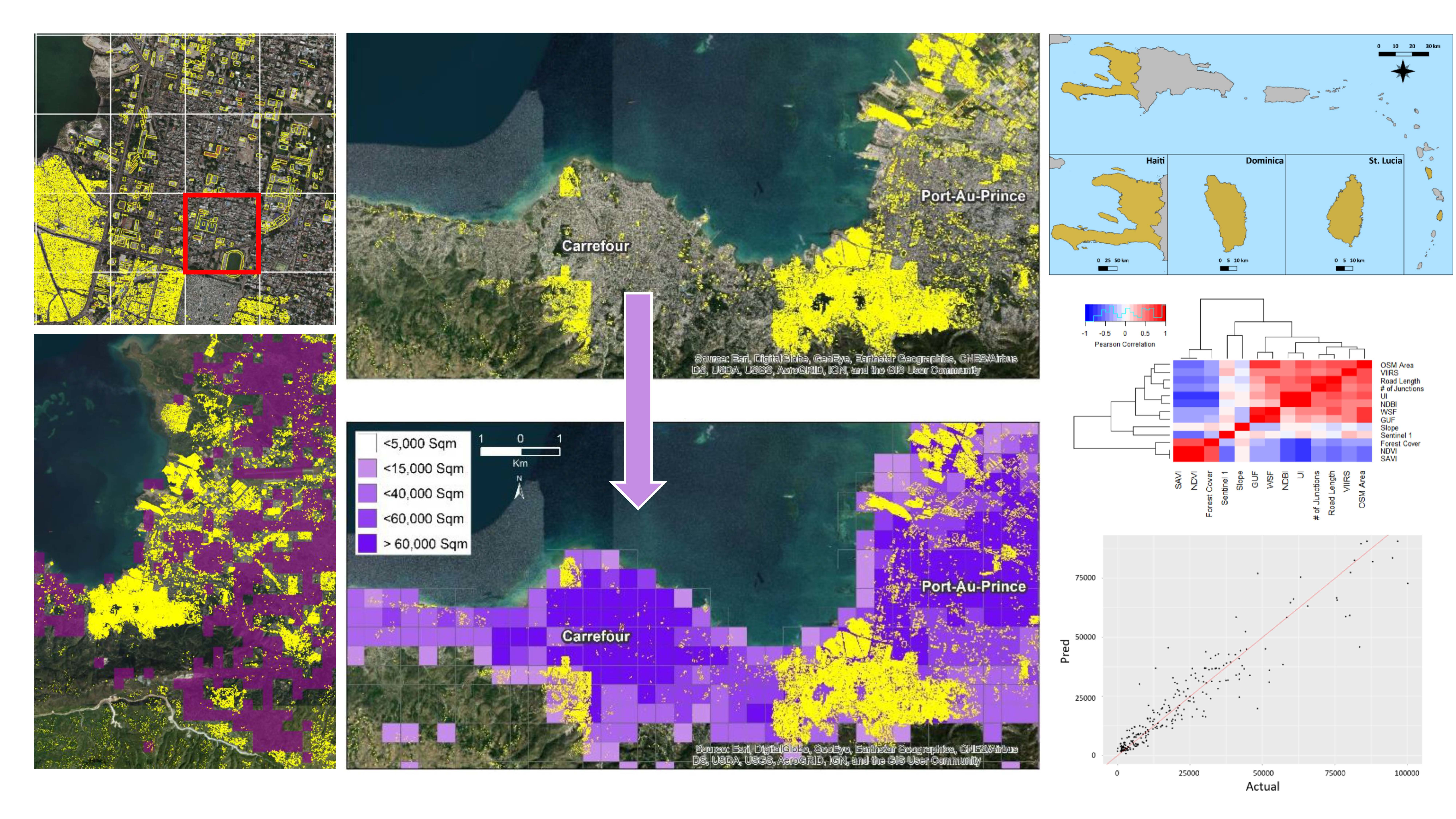
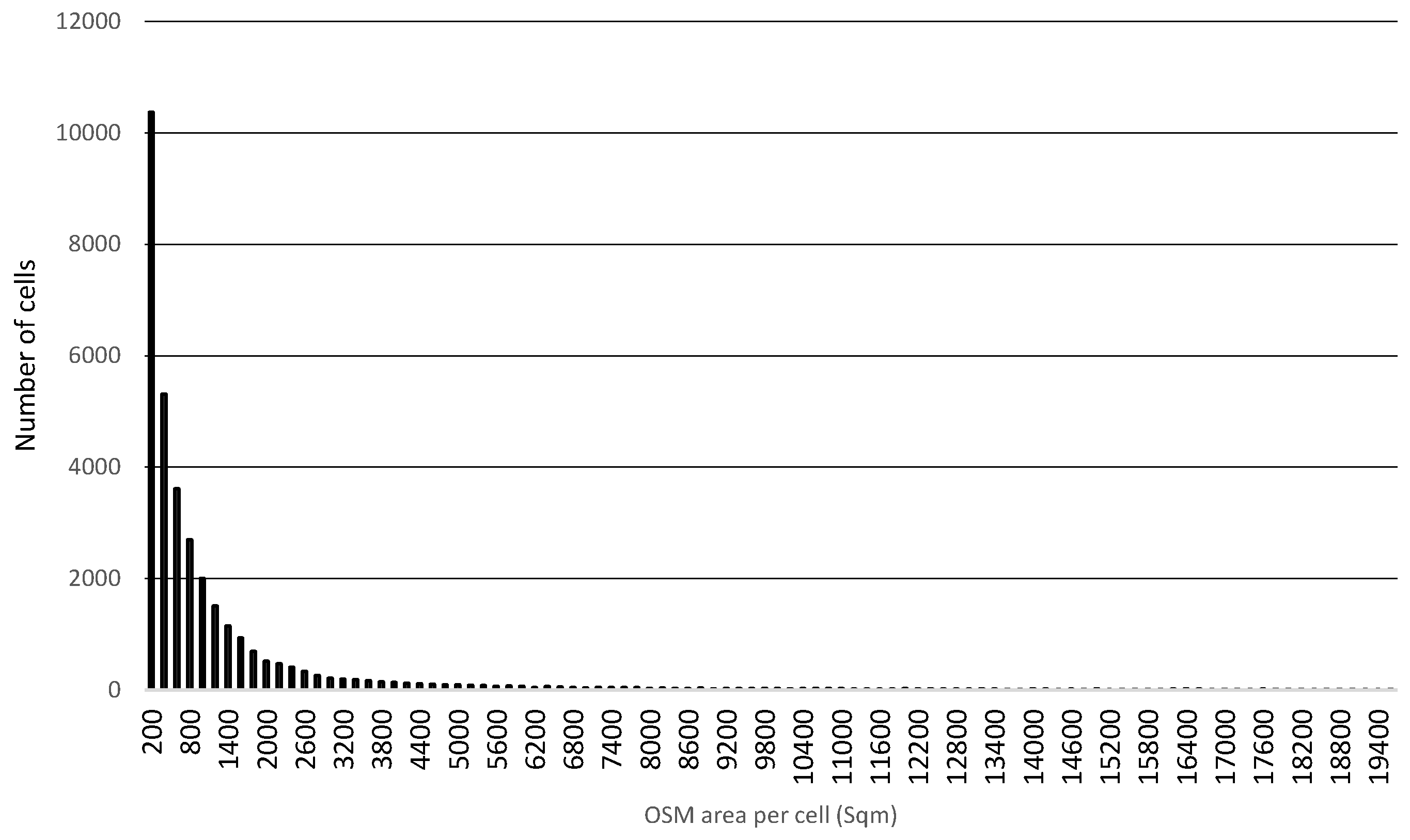
2.1. Study Areas

We demonstrate our methodology in the case of three small island states: Haiti, Dominica and St. Lucia (Figure 1).

2.1.1. Haiti

Located on the western side of Hispaniola Island, Haiti (27,750 km2 in size, with a population of approximately 11.5 million) is the poorest country in the Western Hemisphere, with a Gross Domestic Product (GDP) per capita of US$ 870 [53]. Haiti is highly vulnerable to natural disasters; more than 96% of its population is exposed to different types of natural hazards, particularly hurricane, coastal and riverine flood, and earthquake [53]. More than half of the population lives in cities and towns, a major shift from the 1950s when approximately 90% of Haitians lived in the countryside [54]. Almost all of Haiti‘s 30 major watersheds experience significant flood events, due to intense seasonal rainfall, storm surge in the coastal zones, deforestation and erosion, and sediment-laden river channels [55]. Furthermore, large portions of the country’s population (e.g., in the capital, Port-au-Prince) live in shanty towns built upon steep and exposed hillsides [56]. In 2018 alone, some 2.8 million people were considered to be in need of humanitarian assistance valued at US$ 252.2 million [57].

2.1.2. St. Lucia

A small windward island state located in the Caribbean Sea and the North Atlantic Ocean, St. Lucia (616 km2 in size) has a population of approximately 165,000 [58] and a GDP per capita of US$ 10,315 [59]. St. Lucia is susceptible to numerous natural hazards, including hurricanes, landslides, flooding, and volcanic eruptions. Its terrain consists mainly of mountains and steep slopes in the center of the country due to its volcanic origins with low-lying areas along the coasts [60]. As of 2018, approximately 19% of the population resides in these low-lying areas [61]. In addition, St. Lucia’s economy is highly dependent on two sources: the export of bananas and income from tourism. Both have been negatively impacted recently by natural hazards such as in 2016 when Hurricane Matthew caused 70% of the island to lose power and damaged 80% of the country’s banana plantations [60].

2.1.3. Dominica

Dominica (approximately 74,000 people [62]) is located in Leeward Islands chain in the Lesser Antilles of the Caribbean Sea, approximately 1200 km southeast of Haiti, with large portions of its population residing in the capital Roseau (population 14,700) and Portsmouth (population 5200) [62]. Dominica is vulnerable to a wide range of natural hazards, including hurricanes, intense rainfall, slope instability, volcanic eruptions, seismic activities, and tsunamis [63]. Reflecting a rugged physical topography, most of the population and infrastructure are located on the coast, making the country particularly vulnerable to strong winds and high seas [64]. In September 2017, a Category 5 hurricane Maria hit the country, causing losses and damages worth 226 percent of GDP [65].

2.2. Analytical Framework

The objective of this study is to identify gaps in the completeness of OSM building footprints in three small island states (Haiti, St. Lucia and Dominica) based on remotely sensed measurements and other geospatial features. The procedure involves seven steps.

2.2.1. Step 1: Construct an Artificial Tessellation

We construct an artificial tessellated grid of cells that span each of the countries; each cell is 0.25 square km in size (a total of 136,747 grid cells over Haiti, 2796 grid cells over St. Lucia and 3861 grid cells over Dominica). Each grid cell was treated an independent unit of analysis.

2.2.2. Step 2: Download the Current OSM Building Footprints

We downloaded the most up-to-date OSM data for the three countries (data downloaded in July 2019). For Haiti, we downloaded the data (in a Shapefile format) from Geofabrik (https://www.geofabrik.de/data/download.html). At the time of the analysis, Geofabrik did not have data for Dominica and St. Lucia; thus, we downloaded the data for these countries from overpass turbo (https://overpass-turbo.eu/) in a KML format (this data requires additional pre-processing and we selected OSM features that are labeled as “building=Yes”). At the time of the analysis, there were 930,000 mapped buildings in Haiti, 38,619 mapped buildings in Dominica and 29,412 mapped buildings in St. Lucia.

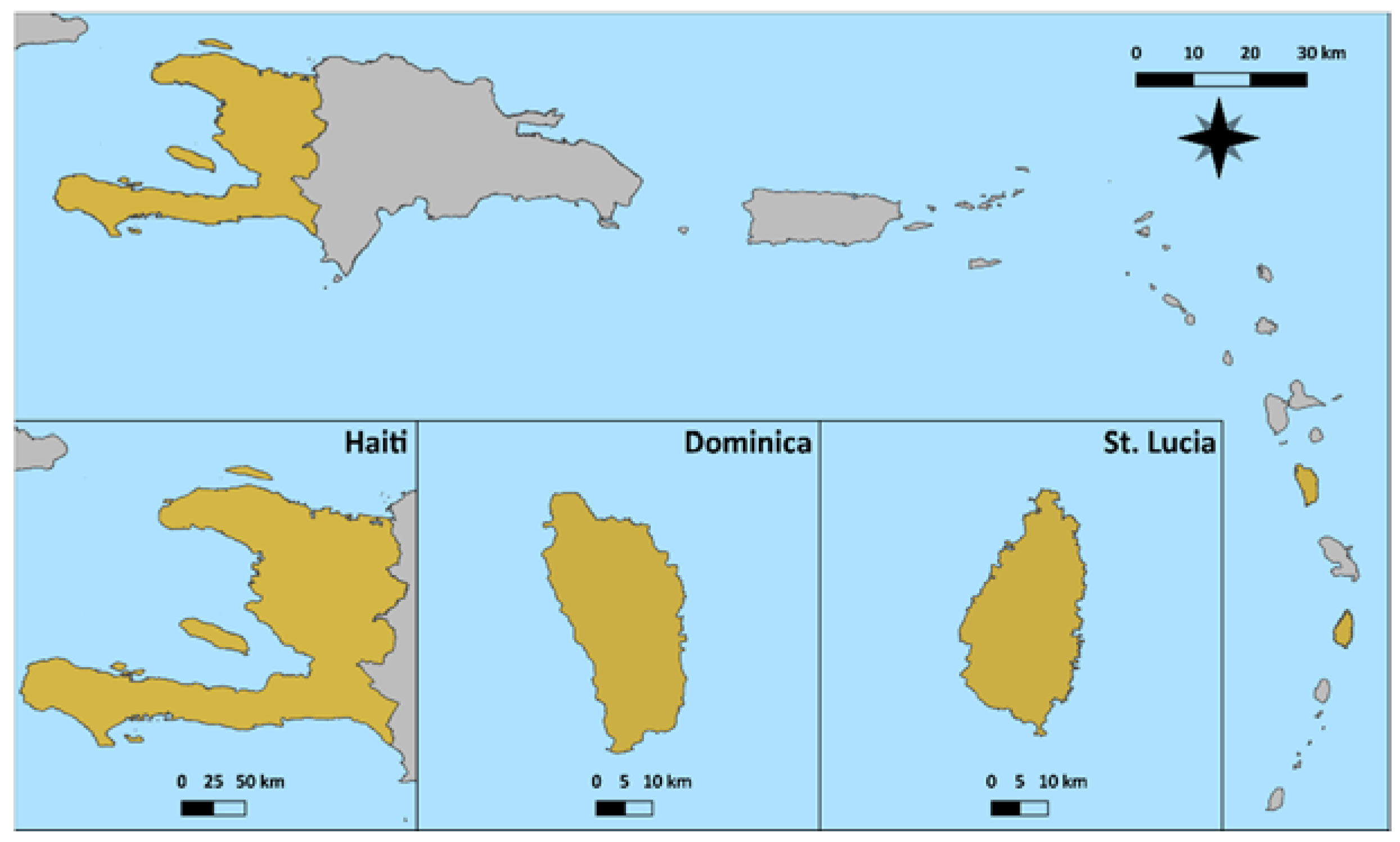
2.2.3. Step 3: Calculate Total Area of OSM Building Footprints in a Grid Cell

We calculated the total area of OSM building footprints in each grid cell. This is the value to be predicted by the explanatory variables (the remotely sensed and geospatial measurements).

2.2.4. Step 4: Preprocess and Aggregate the Remotely Sensed and Geospatial Data

We relied on several predictors (explanatory variables) to estimate the coverage of OSM building footprints in a grid cell and to identify gaps in OSM coverage. We preprocessed the data and aggregated it to the level of a grid cells (Table 1 provides a description of the evaluated explanatory variables and the aggregation measures). The preprocessing, analysis and aggregation of the remotely sensed data were completed by using Google Earth Engine (GEE). GEE is a platform that leverages cloud-computing services to achieve planetary-scale utility and has been previously used for a wide range of applications [66], including mapping population [67,68] and urban areas [69,70].
Nighttime Lights (VIIRS): The Visible Infrared Imaging Radiometer Suite (VIIRS) is one of the key instruments onboard the Suomi National Polar-Orbiting Partnership (Suomi NPP) spacecraft (launched in 2011). VIIRS instrument collects visible and infrared imagery and global observations of land, atmosphere, cryosphere and oceans. This instrument has significant improvements over the capabilities of the former DMSP-OLS [71], notably its availability on a daily basis and higher spatial resolution (up to 500 m at the equator). The VIIRS DNB provides global coverage with 12-hour revisit time. First, we record for each pixel the maximum value of all overlapping pixels (in the same location) in a stack of seven monthly composites (Jan–July) of 2019. Then, for each grid cell, we calculated a Sum of Light (SOL) measure (calculated as the sum of the digital number values of all overlapping pixels in each cell).
Sentinel-2-Derived Spectral Indices: The Copernicus Sentinel-2 mission comprises a constellation of two polar-orbiting satellites that collect multispectral data in 13 spectral bands, with four bands at a spatial resolution of 10 m and 6 bands at a spatial resolution of 20 m. The revisit period of Sentinel-2 is 5 days at the equator. We calculated four remotely sensed measures sensitive to vegetation and built-up land cover: Normalized Difference Vegetation Index (NDVI) [72], Soil Adjusted Vegetation Index (SAVI) [73], Normalized Difference Built-up Index (NDBI) [74] and Urban Index (UI) [75]. For each grid cell, we calculated a per-index sum value of all pixels overlapping with the grid cell.
Sentinel-1 SAR: Sentinel-1 mission comprises a constellation of two polar-orbiting satellites, performing C-band synthetic aperture radar imaging, enabling them to acquire imagery in day and night conditions regardless of the weather. Sentinel-1 has a 12-day repeat cycle, with a spatial resolution down to 5 m. Similarly to [70], we captured the texture of the surface by utilizing Sentinel-1’s C-band (single co-polarization vertical transmit and vertical receive (VV) acquisition mode with an Interferometric Wide Swath (IW) instrument mode, a 250 km swath at 5 m by 20 m spatial resolution (single look)). From each scene, we removed speckle noise and performed radiometric calibration and terrain correction. To create the annual composites, we calculated for each location (pixel) the median value of all overlapping pixels in an entire stack of all scenes captured in 2019. For each grid cell, we calculated the average value of all pixels incorporated within the area of the grid cell.
Slope: To capture the topography of the surface, we used the Global SRTM mTPI dataset (available in GEE in a spatial resolution of 270 m), where a local gradient is calculated for each pixel based on the global SRTM DEM elevation data (30 m resolution). The mTPI distinguishes ridge from valley forms and is calculated using elevation data for each location subtracted by the mean elevation within a neighborhood [76]. For each grid cell, we calculated the average value of all pixels in the grid cell.
Forest Cover: We estimated the extent of forest cover in 2018 based on the Hansen Global Forest Change v1.6 (2000–2018) [77]. First, we defined a pixel as “forest” in the year 2000 if more than 20% of it was covered in 2000 with forest. We recorded pixels that experienced a major event of forest cover loss between 2000 and 2018 and estimate the total area of forest cover in 2018 per grid cell.
Urban Footprints: We relied on two remotely sensed derived products signifying urban and rural settlements that were produced by the Earth Observation Center at DLR: The Global Urban Footprint (GUF) (in a spatial resolution of ~12m) and the World Settlement Footprint (WSF) (in a spatial resolution of ~10m) [78,79,80].
OSM Transportation Network Features: We calculated the total length of OSM roads in a cell and the total number of junctions in a cell as additional potential predictors of OSM-building footprints.

2.2.5. Step 5: Identify Mapped Grid Cells

We adopted a visual interpretation method to visually assess the completeness of OSM building footprints in the grid cells in Haiti and St. Lucia. We achieved this by overlaying the OSM building footprint dataset with the most recent high-resolution base map image (provided by ESRI, updated as of 2019 [81]). We identified grid cells in Haiti and St. Lucia where we assessed that at least 75% of the buildings that are visible in the satellite image have been mapped (we identified 835 grid cells in Haiti and 179 grid cells in St. Lucia). Because the majority area of Dominica has been mapped, we skipped this step in the case of this country.

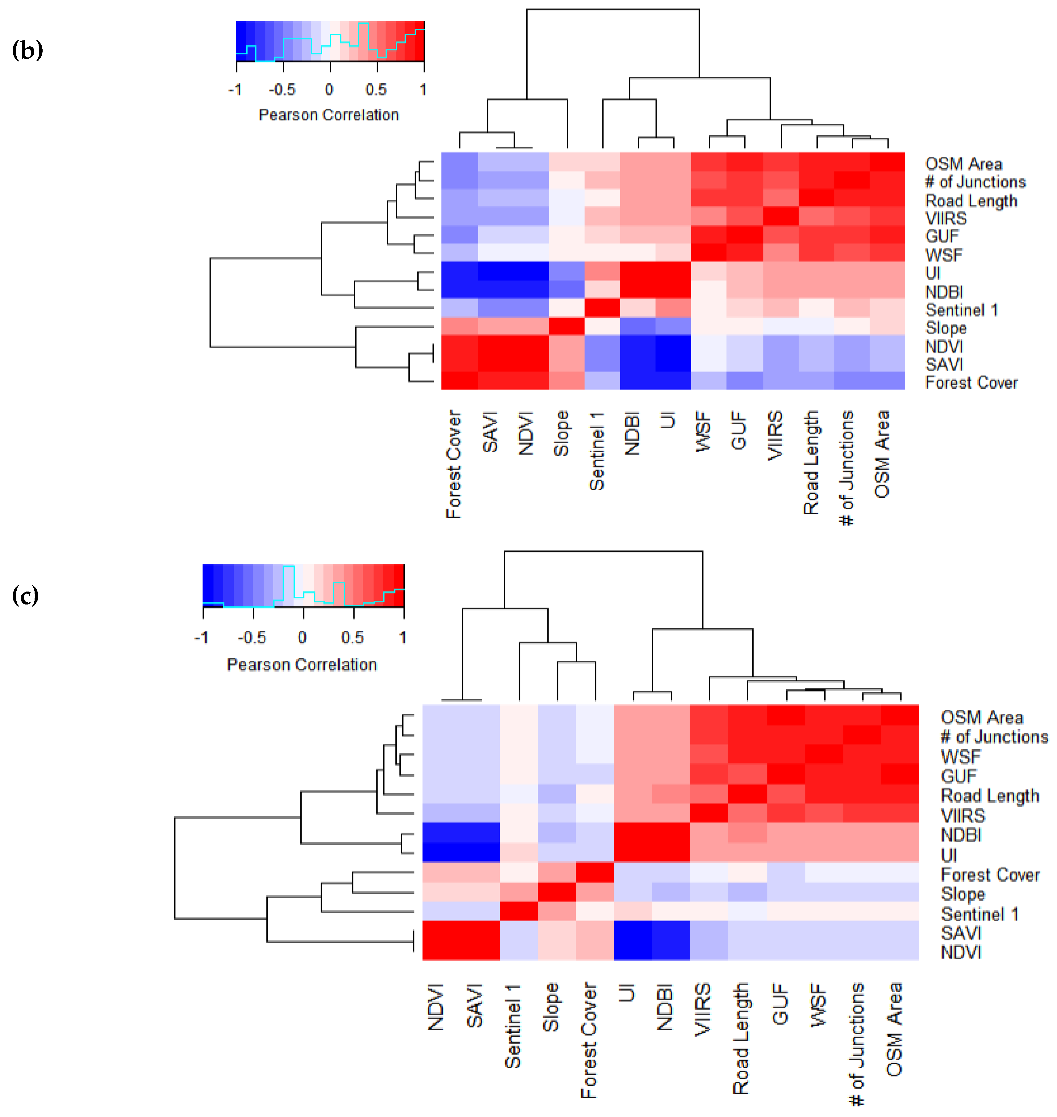
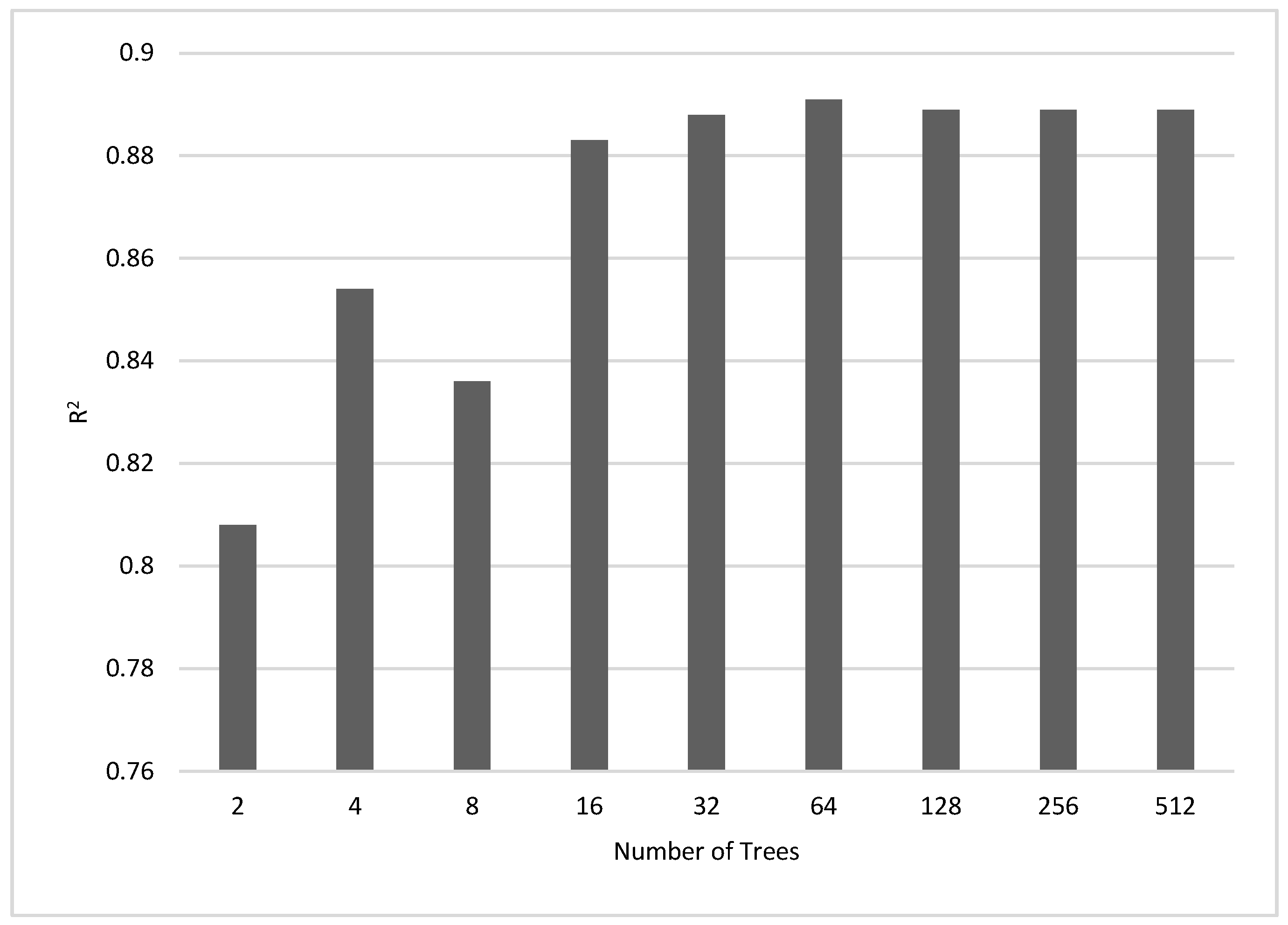
2.2.6. Step 6: Perform Correlation Analysis and Prediction

We evaluated the correlation between the remotely sensed and the geospatial measures (the explanatory variables) and the area of OSM building footprint in a grid cell using a Pearson Correlation Test, and performed an Ordinary Least Squares (OLS) regression to estimate the potential of the variables, combined, to explain the observed variation in the area of OSM building footprints in a grid cell. Additionally, we evaluated the potential of the explanatory variables to predict the area of OSM building footprints in a grid cell using a regression with Random Forests. Random Forests [82] are tree-based models that include k decision trees and p randomly chosen predictors for each recursion. When predicting, for an example, its variables are run through each of the k trees, and the k predictions are averaged through an arithmetic mean. Each tree is trained using a subset of examples from the training set, drawn randomly with replacement, with each node’s binary question determined using a random subset of p input variables. We performed the regression with the 835 grid cells that were visually assessed as being relatively fully mapped (i.e., more than 75% of the buildings in a grid cell are assessed as mapped). To evaluate the accuracy of the prediction, we adopted a fivefold cross-validation method. In each experiment, the examples in one of the data folds were left out for testing and the examples in the remaining four folds were used to train the model. The performance quality of the trained model was tested on the examples in the left-out fold, and the overall performance measure is then averaged over the five folds. We assessed the classification accuracy with a different number of decision trees: 2, 4, 8, 16, 32, 64, 128, 256 and 512, with minimum size of terminal nodes set to 5.

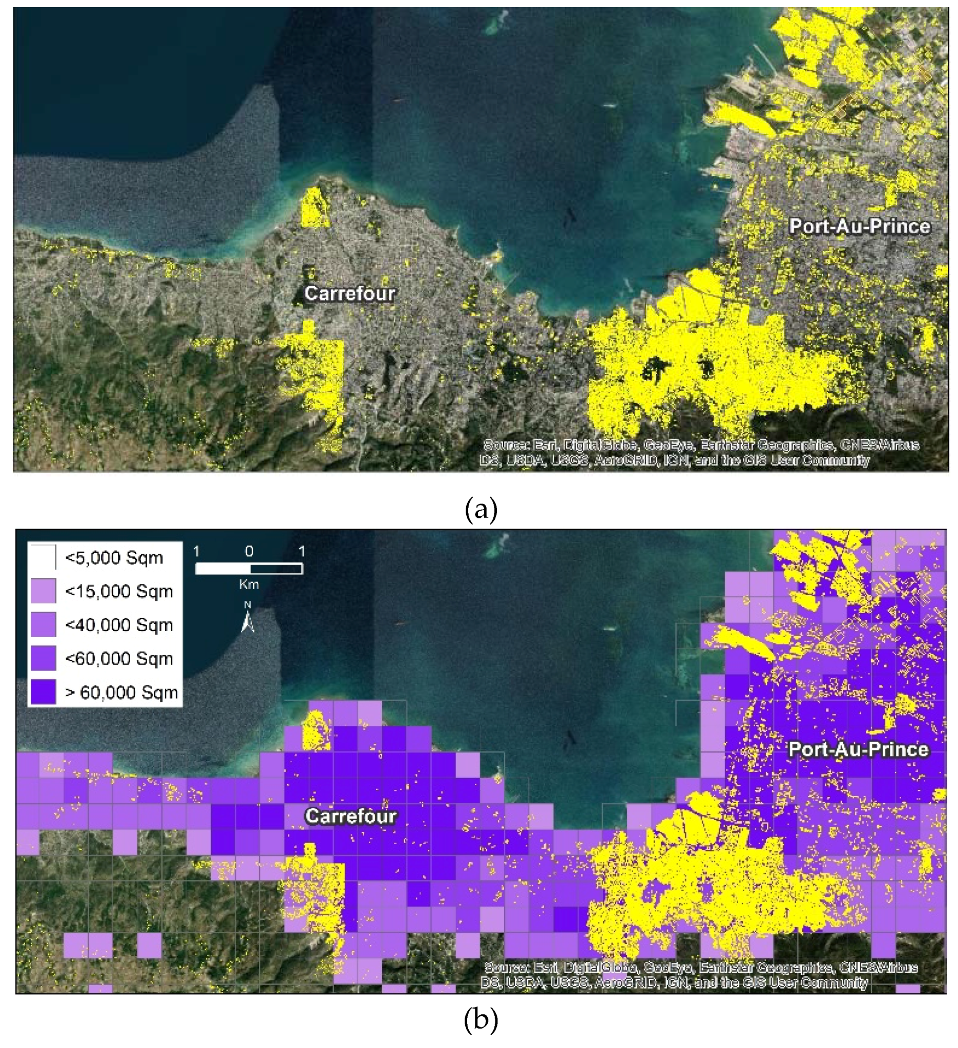
2.2.7. Step 7: Predict the Coverage of OSM-Building Footprints in Each Entire Country

We used either the grid cells that are visually assessed as relatively fully mapped (in the case of Haiti and St. Lucia) or all the grid cells (in the case of Dominica) as references for the training of Random Forest Regression and to predict the area of OSM building footprints over the entire grid cells in each country. We identified the grid cells that were predicted to incorporate OSM building footprints, but were not yet mapped.

3. Results

An examination of the 136,747 cells spanning Haiti shows that only 25.1% of the cells have at least one mapped building, and only 512 of the 136,747 cells have more than 10% of their area covered with building footprints (Figure 2 shows a histogram of the distribution of OSM building footprints per cell). On average, there are 27.5 buildings in a cell (Std = 83.4); 1530 of the cells (i.e., only 1.1% of the cells spanning Haiti) incorporate more than 100 mapped buildings. In comparison, 8.15% and 6.84% of the cells incorporate built-up land cover according to WSF and GUF, respectively.
As discussed above, a visual examination of the completeness of OSM building footprints over Haiti suggests that large portions of the island remain unmapped (Figure 3a). Figure 3b,c show, as an illustration, the coverage of OSM building footprints in the capital of Haiti, Port-au-Prince and Carrefour, and in the adjacent Carrefour commune. While buildings in many areas within these cities have been mapped, large portions are still not fully mapped. We observe that densely mapped zones of Port-au-Prince co-exist alongside zones that remain entirely unmapped (Figure 3c), a visual pattern that may result from the episodic engagement of community mapping volunteers and the definition of mapping ‘tasks’ on a neighborhood scale through OSM editing tools. Moreover, significant parts in northern Haiti are not mapped (Figure 4), including, for example, the cities Gonaïves and Cap-Haitien.
A Pearson correlation test indicated a significant (p < 0.01) correlation between the total area of OSM building footprints in a grid cell and several of the examined explanatory variables. As expected, there was a positive and significant correlation between the area of OSM building footprints in a grid cell and the total area of built-up land cover, according to WSF and GUF (r = 0.73 and 0.71, respectively, p < 0.01) as well as with nighttime lights (VIIRS SOL) (r = 0.63, p < 0.01). We find a significant (p < 0.01) correlation between OSM building footprints area in a grid cell with the four Sentinel-2 spectral indices, indicated by a positive correlation with UI and NDBI (r = 0.59 and r = 0.47) and a negative correlation with both SAVI and NDVI (r = −0.53).
We identified 835 grid cells where, according to a visual assessment, at least 75% of the buildings that were visible in the satellite image are mapped in OSM (Figure 5 shows examples of grid cells where more than 75% of the structures are mapped). The correlation between the area of OSM building footprints in a grid cell and the examined predictors was higher compared to the previous experiment, where all the grid cells (i.e., 136,747 grid cells) were considered (for example, r = 0.78 and r = 0.65 with WSF and VIIRS and r = 0.61 and r = −0.55 with UI and SAVI, respectively) (Table 2), which is likely due to the fact that large portions of the country are not mapped (i.e., there are grid cells that lack OSM coverage while actually populated and exhibit LULC characteristics of populated areas). As expected, there were also similarities and correlations between some of the explanatory variables. Figure 6a presents pairwise correlation coefficients between the explanatory variable (variables are ordered according to a hierarchical clustering). The explanatory variables form several similarity clusters: a cluster composed out of vegetation spectral indices (NDVI, SAVI) and forest cover (which are positively correlated with each other), and a cluster composed out of built-up land cover spectral indices (NDBI, UI), together with VIIRS, WSF, GUF, and OSM road network features. As expected, there is a negative and significant correlation between the vegetation and the built-up land cover spectral indices. The dendrogram shown in the figure further highlights hierarchical clusters formed between the variables, notably, OSM area and VIIRS, UI and NDBI, NDVI and SAVI, and road length and number of junctions in a grid cell.
An Ordinary Least Squares (OLS) regression shows that nine of the variables together explain up to 82% of the variation of OSM building footprints area in a grid cell (R2 = 0.82, F(12,822) = 323.20, p < 0.01) (Table 3). We evaluated the contribution of four types (groups) of features to the model fit using a stepwise regression analysis: (1) only GUF and WSF; (2) with the addition of nighttime lights (VIIRS); (3) with the addition of further remotely sensed measures and derived products; (4) with the addition of OSM road network features. The results show an improvement of the model fit with the addition of each of the predictive variables groups (Table 4). While GUF and WSF together explain 66% of the fit, the addition of nighttime lights improves the fit of the model (indicated by explanation of up to 76% of the variation). The addition of further remotely sensed measures (i.e., Sentinel-2-derived spectral indices, slope, texture and forest cover) improves the model fit by a further 5% (up to 81% of the variation). With the addition of OSM transportation network features the fit of the model improves marginally to around 82%.

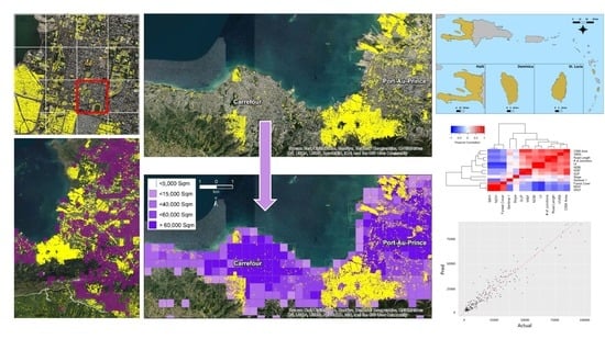
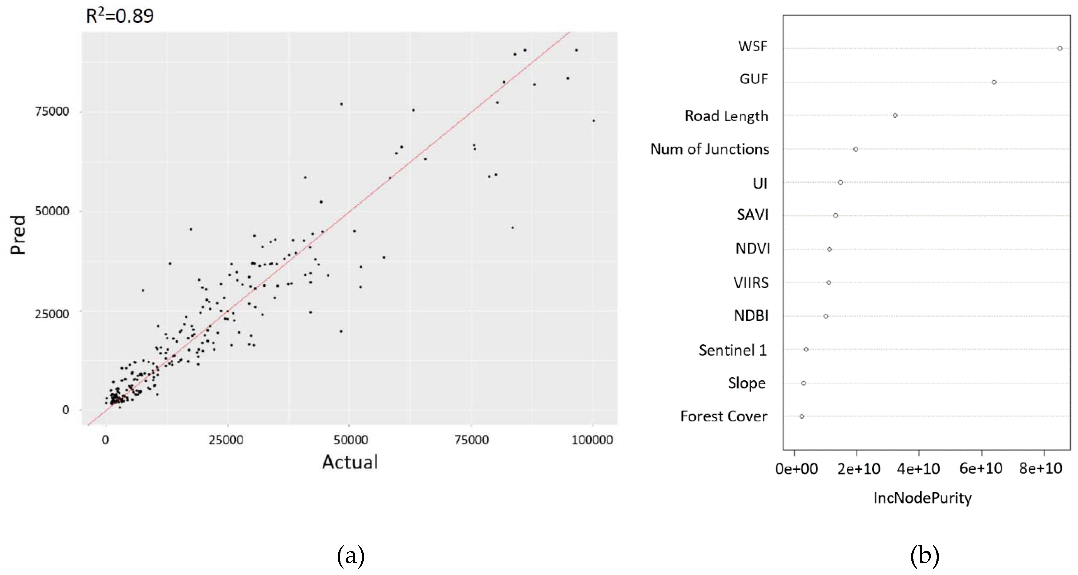
3.1. Prediction of OSM Building Footprint Coverage

The results above indicate that the area of OSM building footprints in a grid cell can be explained by several of the remotely sensed and geospatial explanatory variables. To evaluate the potential of these variables to predict the area of OSM building footprints in a cell, we performed a regression with Random Forests.
Random Forest regression predicts up to 89% of the variation of OSM building footprints in a grid cell. Performance improves with the addition of decision trees up to 64 trees, for example, from 81% to 89% of the predicted area (with 2 and 64 decision trees, respectively, Figure 7). Figure 8 presents a comparison between the actual and the predicted area of OSM building footprints in a grid cell (regression with 64 decision trees) (Figure 8a). The two most important variables to the model are WSF and GUF, followed by OSM road network features and Sentinel-2 derived spectral indices (indicated by variable importance sensitivity (lncNodePurity), Figure 8b).
We use the Random Forest model to predict the area of OSM building footprints over all the grid cells in Haiti (i.e., we train the model with the 835 grid cells that were assessed as relatively fully mapped and predict for the coverage over the entire dataset). Figure 10b shows the predicted area of OSM building footprints per grid cell over Haiti. The results highlight large portions in Haiti that have not yet been mapped (e.g., for example, the northern cities Gonaives and Cap-Haitien) as well as patches of unmapped grid cells around major cities (e.g., Port-au-Prince). This analysis allows us to identify areas (grid cells) that are predicted to incorporate large areas of building footprints but are not mapped (Figure 9).
A visual examination shows that the predicted coverage of OSM building footprints (Figure 10b) corresponds more closely with the distribution of built-up land cover (according to GUF, for example) and nighttime lights (VIIRS) (Figure 10c,d, respectively) than compared to the current distribution of OSM building footprints (Figure 10a).
To further evaluate the accuracy of the model, we perform an OLS regression analysis using the entire Haiti dataset (i.e., 136,747 grid cells). We find that the remotely sensed measurements explain up to 89% of the variation of the predicted area of OSM building footprints in all the grid cells spanning Haiti (R2 = 0.89, F(12,136,734) = 90,690, p < 0.01). In comparison, these indicators explain only 48% of the variation of the current area of OSM building footprints in the Haiti dataset (R2 = 0.48, F(12,136,734) = 10,330, p < 0.01).
Finally, in order to identify grid cells that are predicted to incorporate building footprints but are actually not mapped, we calculated the ratio between the actual and the predicted area of OSM building footprint in a grid cell (calculated as the predicted area of OSM building footprints in a grid cell divided by the actual area of OSM building footprints in a grid cell) (Figure 11a,c). This analysis allows us to identify grid cells where the ratio between the predicted and the actual area of OSM building footprint in a grid cell is low (Figure 11b,d), highlighting grid cells that require mapping.

3.2. Evaluation of the Method in the Case of Dominica and St. Lucia

The results above suggest the potential of several remotely sensed indicators to predict the coverage of OSM building footprints, at least in the case of Haiti. In order to assess the validity of the method, we performed further analysis in the case of two additional small island states: Dominica and St. Lucia. A visual examination suggests that the coverage of OSM building footprints in Dominica is relatively complete, while large portions of St. Lucia remain unmapped. Areas lacking OSM building footprints include parts of the capital, Castries, and the second-largest town, Vieux Fort (Figure 12). These two areas account for approximately 49% of the population of St. Lucia (64,654 and 16,624 people, respectively [83]).
Similar to the methodology described in the case of Haiti, we created a fishnet of grid cells, 0.25 km2 in size, spanning the two islands. In the case of Dominica, we found a high positive and significant correlation between the area of OSM building footprints in a grid cell and several explanatory variables. We found a high positive correlation with GUF, number of junctions and WSF (between r = 0.90 and r = 0.91, p < 0.01 for both). The correlation between the area of OSM building footprints and VIIRS is a bit lower (r = 0.75, p < 0.01). With Sentinel-2-derived spectral indices, this correlation ranges between r = 0.35 and r = 0.38 (with UI and NDBI, respectively, p < 0.01 for both). An OLS regression analysis reveals that together, these variables explain 92% of the variation of OSM building footprint area in a grid cell (R2 = 0.92, F(12,3846) = 3848, p < 0.01). Random Forest regression (with 64 decision trees) results in similar trends, indicated by a high accuracy rate of 88% (regression accuracy assessed using fivefold cross-validation).
In the case of St. Lucia, when the analysis was done with the entire dataset of grid cells over the country (i.e., N = 2781), the correlation between the area of OSM building footprints, GUF and WSF ranges between 0.70 and 0.75 (p < 0.01) and there is a lower correlation between OSM building footprints area and VIIRS (r = 0.58, p < 0.01). Together, the predictors explain only 66% of the variation is OSM building footprints (R2 = 0.66, F(12,2783) = 464.6, p < 0.01). We relate the lower fit of the model to the fact that large portions of the country have not been mapped. Thus, we visually assessed the completeness of OSM building footprints in St. Lucia grid cells and identified 179 grid cells in which we could assess that more than 75% of their area is mapped. With these visually assessed grid cells, the fit of the model improved, and together, the predictors explain 92% of the variation of OSM building footprint area (R2 = 92%, F(12,166) = 166.4, p < 0.01). Random Forest regression (with 64 decision trees) results in a similar accuracy rate (R2 = 92%) (Table 5).
Finally, we use Random Forest to predict the area of OSM building footprints in each of the countries. Figure 13 presents the predicted area of OSM building footprint in St. Lucia. Unmapped areas include, for example, areas surrounding the capital of Castries. The central part of the city is densely mapped while its adjacent neighborhoods lack coverage. Large swaths of the surrounding areas of Charlotte, Vigie, and Bisee completely lack OSM building footprints.

4. Discussion

In recent decades, natural disasters have been responsible for an estimated 0.1% of global deaths, killing on average 60,000 people per year [84]. In the last two decades alone, developing countries have accounted for more than half of all reported casualties [85]. Natural disasters often cause significant damage to communities, infrastructure and the environment, and require immediate intervention and implementation of appropriate measures aiming to save lives.
Accurate and easily accessible geospatial information is key for an effective disaster risk management cycle and for informed decision-making during humanitarian response [86]. The increasing availability of geospatial information is revolutionizing disaster research and emergency management. Until recently, much of this essential geospatial information was proprietary, scarce and in many cases, unavailable during significant disasters.
In the last decade, OSM has repeatedly been shown to be highly suitable for disaster mapping and management. Despite the continuous efforts to improve completeness of the OSM database, large portions of the world remain unmapped, especially in countries that are prone to natural hazards, reflecting limited internet speed connectivity, limited availability of GPS devices, lack of technologically skilled volunteers and limited awareness of VGI technologies [18].
Several methods have been proposed to assess the completeness of the OSM database, including evaluation of the completeness of street networks, land use and buildings; many of them rely on external datasets for accuracy and completeness estimation. The increased availability of free and open-source remotely sensed data can be utilized to identify mapping gaps in OSM datasets, find locations that require mapping, and help prioritize and plan mapping campaigns and efforts. Although several applications have recently been proposed to predict the coverage of OSM by means of remotely sensed derived products (such as WorldPop) [87], to the best of our knowledge, no study has yet evaluated the potential use of remotely sensed measurements to predict the completeness of OSM features.
In this study, we demonstrate a methodology to identify areas where building footprints have not yet been mapped in OSM dataset. The methodology relies on remotely sensed measurements and derived products and geospatial information related to the road network to predict the completeness of OSM building footprints in three small island states (Haiti, Dominica and St. Lucia).
In the case of Haiti, the results show that large portions of the country are still unmapped, despite the continued mapping efforts to maintain a full and up-to-date map while also keeping pace with the changing socio-physical characteristics of the country and to aid response and recovery in future disasters [88]. We find that in the case of the three countries, the coverage of OSM building footprints is significantly correlated with several remotely sensed measures and indicators. As expected, the coverage is positively correlated with the distribution of built-up land cover (indicated by a Pearson correlation coefficient of between r = 0.78 and r = 0.91 in the case of Haiti and Dominica, respectively). To some extent, this is not surprising, and previous studies have already shown the potential of remotely sensed derived products to predict the coverage of OSM building footprints [87]. However, a limiting factor in utilization of remotely sensed derived products is that their availability varies in space and time and these products are not always updated on a regular basis. In this study, we demonstrate the potential use of free and open-source remotely sensed indicators to estimate the coverage of OSM building footprints. We show that the intensity of nighttime lights luminosity (measured by VIIRS) is highly correlated with the area of OSM building footprints (indicated by a Pearson correlation coefficient of between r = 0.65 and r = 0.75 in the case of Haiti and Dominica, respectively). This finding aligns with previous studies showing that the intensity of nighttime lights is closely correlated with anthropogenic activities and with changes in the distribution of built-up land cover [89,90], as well as with the distribution of geographical features, such as the density of the road network [91]. Further, we show that remotely sensed spectral indices signifying the distribution of vegetation (NDVI, SAVI) and built-up land cover (NDBI, UI) are also correlated with the distribution of OSM building footprints. While previous studies propose to utilize vegetation spectral indices (e.g., NDVI) to estimate the completeness of urban green spaces mapping in OSM [92], we show that these indices are also significantly correlated with the coverage of OSM building footprints.
Because different sensors record distinct characteristics of the land (e.g., brightness, temperature, height, density, texture), data fusion techniques that exploit the best characteristics of each type of sensor have become a valuable procedure in remote-sensing analysis, including for urban applications [70,93] and in mapping the built-up land cover [69]. In this study, we show that the combined effect of the explanatory variables explains between 92% and 94% of the variation in the area of OSM building footprints, exceeding the effect of each predictor by itself. We show that in the case of Haiti, the addition of nighttime lights to built-up land cover classification products (GUF, WSF) improves the fit of the model by 10%, and that with the addition of remotely sensed measures, the fit of the model improves by 5%. Although land cover characteristics are often related to nighttime light luminosity (for example, vegetation density decreases while luminosity increases from the rural area to the urban core), fusing nighttime and daytime remotely sensed measures allows for an increase in the separability between urban and nonurban land [94]. Fusing daytime and nighttime measurements enable feature complementation and compensation for the limitation of single data sources in extracting urban information [95].
We also perform a Random Forest Regression to predict the area of OSM building footprints in a cell and find that the regression explains between 88% and 94% of the variation (in Dominica and Haiti, respectively). Previous studies suggest that the number of decision trees of the Random Forest is generally proportional to the model’s accuracy [96], although they show mixed results for the optimal number of trees in the decision tree. The number varies between 10 [97] and 150 trees [98]. Here, we find that with Random Forests, accuracy improves up to 64 decision trees and then moderately decreases as the number of trees increases.
Finally, we demonstrate the potential of our approach to identifying mapping gaps, or areas that lack OSM coverage. We do this by training the model with the grid cells that are visually assessed as relatively completely mapped and use the trained model to predict the coverage of OSM building footprints throughout the countries. We capture grid cells that lack OSM building footprints coverage (i.e., grid cells where the predicted coverage of OSM building footprints largely exceeds the actual coverage). These grid cells represent locations where mapping efforts could potentially be targeted.
To summarize, VGI contributions, especially in developing countries, tend to be made in spurts, for example in response to a specific trigger, such as a natural disaster or humanitarian crisis, rather than as a regular, continuous process [13]. Because OSM datasets rely on volunteers, the completeness and mapping efforts vary in space and time. There is a need for a systematic tool that would guide and prioritize mapping efforts and mapping campaigns. As more and more remotely sensed data become available to the research community, our study extends the existing literature by demonstrating how they could be leveraged to conduct novel, and critical, large-scale assessments of the completeness of the OSM database, especially in areas at high risk to natural disasters.
We note a few limitations to this study. First, we demonstrate our methodology in the case study of three small island states, which, at least to some extent, are characterized by relatively similar geographical conditions and characteristics. An extension of this study would evaluate our methodology in additional countries characterized by diverse geographical conditions (topography, land cover, land use, etc.). Second, in order to create the training examples for the model and to evaluate the relation between the explanatory variables and the area of OSM building footprints, we created a relatively small dataset of examples (grid cells), which were visually assessed using a subjective visual interpretation method as relatively fully mapped. By its nature, visual interpretation may be subject to idiosyncratic variation across individuals performing the manual classification. An extension to this study would leverage the crowd to create an extensive dataset of grid cells visually assessed and mapped and would account for an agreement between the interpreters. Third, the analysis presented in this study was done at a single point in time. By its nature, the OSM database is continuously updated and is dynamic, while simultaneously, new remotely sensed measurements are being collected. An extension to this study would account for these changes in time and evaluate the completeness of OSM building footprints on an ongoing basis as new data becomes available.
Extensions to our approach may improve the identification of areas that lack completed OSM coverage by accounting for additional inputs; for example, socioeconomic variables (including WorldPop, Facebook’s High Resolution Settlement Layer (HRSL) and additional physical/geographical characteristics and spectral indices). Further extensions to our approach may also include the application of learning algorithms and evaluation with various tuning parameters of the classifiers and the fit models.

5. Conclusions

Globally, there has been an increase in the frequency and impacts of major natural disaster events; in the next century, it is likely that climate change will amplify the number and severity of such disasters. While accurate and timely geospatial information is vital for the full cycle of disaster risk management, this data is not always available for the disaster management community when disasters occurs. Although VGI platforms, specifically OpenStreetMap (OSM), show great potential to support humanitarian mapping tasks, gaps in VGI data remains a major concern [99]. There is an increasing need for a fully automatic tool that would allow to identify areas that lack a complete mapping of OSM features—especially in areas prone to hazard events. While previous studies have utilized OSM data as reference for classification of built-up land cover with satellite imagery [100,101,102,103] here we show the potential use of publicly available, remotely sensed data as predictors of the spatial coverage of OSM building footprints. The tool and methodology we present here are time-efficient and scalable.
An extension to our approach may improve the accuracy of the prediction of OSM building footprints area by adding additional remotely sensed measures. Incorporating additional datasets, such as newly developed VIIRS nighttime light products, socioeconomic variables, additional land cover and land use classification schemes may offer opportunities to improve the accuracy of the prediction.

Author Contributions

R.G. designed the experiments and the methodology with N.J. and J.M., implemented the experiment and wrote the manuscript. J.M. and N.J. helped to carry out and implement the experiment and improve the manuscript. All authors have read and agreed to the published version of the manuscript.

Funding

This research was funded by the Global Facility for Disaster Reduction and Recovery under the Small Island States Resilience Initiative.

Acknowledgments

We thank Brad Bottoms for the excellent help throughout this research.

Conflicts of Interest

The authors declare no conflicts of interest.

References

  1. WHO. Available online: https://www.who.int/environmental_health_emergencies/natural_events/en/ (accessed on 1 November 2019).
  2. FAO. Available online: http://www.fao.org/resilience/areas-of-work/natural-hazards/en/ (accessed on 1 November 2019).
  3. Munang, R.; Thiaw, I.; Alverson, K.; Liu, J.; Han, Z. The role of ecosystem services in climate change adaptation and disaster risk reduction. Curr. Opin. Environ. Sustain. 2013, 5, 47–52. [Google Scholar] [CrossRef]
  4. Brown, P.; Daigneault, A.J.; Tjernström, E.; Zou, W. Natural disasters, social protection, and risk perceptions. World Dev. 2018, 104, 310–325. [Google Scholar] [CrossRef] [PubMed]
  5. Shen, S.; Cheng, C.; Song, C.; Yang, J.; Yang, S.; Su, K.; Yuan, L.; Chen, X. Spatial distribution patterns of global natural disasters based on biclustering. Nat. Hazards 2018, 92, 1809–1820. [Google Scholar] [CrossRef]
  6. Fairbairn, T.I. Economic Consequences of Natural Disasters Among Pacific Island Countries. Pac. Econ. Bull. 1998, 13, 2. [Google Scholar]
  7. Van Beynen, P.; Akiwumi, F.A.; Van Beynen, K. A sustainability index for small island developing states. Int. J. Sustain. Dev. World Ecol. 2018, 25, 99–116. [Google Scholar] [CrossRef]
  8. Goodchild, M.F. Citizens as voluntary sensors: Spatial data infrastructure in the world of Web 2.0. Int. J. Spat. Data Infrastruct. Res. 2007, 2, 24–32. [Google Scholar]
  9. Kawasaki, A.; Berman, M.L.; Guan, W. The growing role of web-based geospatial technology in disaster response and support. Disasters 2013, 37, 201–221. [Google Scholar] [CrossRef]
  10. Poorazizi, M.; Hunter, A.; Steiniger, S. A volunteered geographic information framework to enable bottom-up disaster management platforms. ISPRS Int. J. Geo-Inf. 2015, 4, 1389–1422. [Google Scholar] [CrossRef] [Green Version]
  11. Chen, H.; Zhang, W.C.; Deng, C.; Nie, N.; Yi, L. Volunteered Geographic Information for Disaster Management with Application to Earthquake Disaster Databank & Sharing Platform. IOP Conf. Ser. Earth Environ. Sci. 2017, 57, 012015. [Google Scholar]
  12. Mirbabaie, M.; Stieglitz, S.; Volkeri, S. Volunteered geographic information and its implications for disaster management. In Proceedings of the 2016 49th Hawaii International Conference on System Sciences (HICSS), Kauai, HI, USA, 5–8 January 2016. [Google Scholar]
  13. Mahabir, R.; Stefanidis, A.; Croitoru, A.; Crooks, A.T.; Agouris, P. Authoritative and Volunteered Geographical Information in a Developing Country: A Comparative Case Study of Road Datasets in Nairobi, Kenya. ISPRS Int. J. Geo-Inf. 2017, 6, 24. [Google Scholar] [CrossRef]
  14. Haklay, M.; Weber, P. Openstreetmap: User-generated street maps. IEEE Pervasive Comput. 2008, 7, 12–18. [Google Scholar] [CrossRef] [Green Version]
  15. Neis, P.; Zielstra, D. Recent developments and future trends in volunteered geographic information research: The case of OpenStreetMap. Future Internet 2014, 6, 76–106. [Google Scholar] [CrossRef] [Green Version]
  16. Schelhorn, S.-J.; Herfort, B.; Leiner, R.; Zipf, A.; De Albuquerque, J.P. Identifying elements at risk from OpenStreetMap: The case of flooding. In Proceedings of the 11th International ISCRAM Conference, University Park, PA, USA, 18–21 May 2014. [Google Scholar]
  17. Poiani, T.H.; dos Santos Rocha, R.; Degrossi, L.C.; de Albuquerque, J.P. Potential of collaborative mapping for disaster relief: A case study of OpenStreetMap in the Nepal earthquake 2015. In Proceedings of the 2016 49th Hawaii International Conference on System Sciences (HICSS), Kauai, HI, USA, 5–8 January 2016. [Google Scholar]
  18. Latif, S.; Islam, K.R.; Khan, M.M.I.; Ahmed, S.I. OpenStreetMap for the disaster management in Bangladesh. In Proceedings of the 2011 IEEE Conference on Open Systems, Langkawi, Malaysia, 25–28 September 2011. [Google Scholar]
  19. Palen, L.; Soden, R.; Anderson, T.J.; Barrenechea, M. Success scale in a data-producing organization: The socio-technical evolution of OpenStreetMap in response to humanitarian events. In Proceedings of the Proceedings of the 33rd Annual ACM Conference on Human Factors in Computing Systems, Seoul, Korea, 18–23 April 2015. [Google Scholar]
  20. Eckle, M.; Herfort, B.; Yan, Y.; Kuo, C.-L.; Zipf, A. Towards using Volunteered Geographic Information to monitor post-disaster recovery in tourist destinations. In Proceedings of the ISCRAM, 21–24 May 2017; Available online: https://www.imt.fr/en/events/event/iscram-2017-international-conference-on-information-systems-for-crisis-response-and-management-albi-a-mines-albi-2/ (accessed on 25 December 2019).
  21. Taylor, L.N. Digital Humanities Tools for Disaster Response: Hosting Mapathons and Telling Our Stories. Available online: https://uwispace.sta.uwi.edu/dspace/handle/2139/45647 (accessed on 25 December 2019).
  22. Parr, D.A. The production of volunteered geographic information: A study of OpenStreetMap in the United States. Available online: https://digital.library.txstate.edu/bitstream/handle/10877/5776/PARR-DISSERTATION-2015.pdf?sequence=1&isAllowed=y (accessed on 25 December 2019).
  23. Anderson, J.; Sarkar, D.; Palen, L. Corporate Editors in the Evolving Landscape of OpenStreetMap. ISPRS Int. J. Geo-Inf. 2019, 8, 232. [Google Scholar] [CrossRef] [Green Version]
  24. Herfort, B.; Li, H.; Fendrich, S.; Lautenbach, S.; Zipf, A. Mapping Human Settlements with Higher Accuracy and Less Volunteer Efforts by Combining Crowdsourcing and Deep Learning. Remote Sens. 2019, 11, 1799. [Google Scholar] [CrossRef] [Green Version]
  25. Scholz, S.; Knight, P.; Eckle, M.; Marx, S.; Zipf, A. Volunteered Geographic Information for Disaster Risk Reduction-The Missing Maps Approach and Its Potential within the Red Cross and Red Crescent Movement. Remote Sens. 2018, 10, 1239. [Google Scholar] [CrossRef] [Green Version]
  26. Barrington-Leigh, C.; Millard-Ball, A. The world’s user-generated road map is more than 80% complete. PLoS ONE 2017, 12, e0180698. [Google Scholar] [CrossRef] [Green Version]
  27. Jacobs, C.; Zipf, A. Completeness of citizen science biodiversity data from a volunteered geographic information perspective. Geo-Spat. Inf. Sci. 2017, 20, 3–13. [Google Scholar] [CrossRef] [Green Version]
  28. Hecht, R.; Kunze, C.; Hahmann, S. Measuring Completeness of Building Footprints in OpenStreetMap over Space and Time. ISPRS Int. J. Geo-Inf. 2013, 2, 1066–1091. [Google Scholar] [CrossRef]
  29. Mashhadi, A.; Quattrone, G.; Capra, L. The Impact of Society on Volunteered Geographic Information: The Case of OpenStreetMap. In OpenStreetMap in GIScience: Experiences, Research, and Applications; Jokar Arsanjani, J., Zipf, A., Mooney, P., Helbich, M., Eds.; Lecture Notes in Geoinformation and Cartography; Springer International Publishing: Cham, Germany, 2015; pp. 125–141. [Google Scholar]
  30. Quattrone, G.; Mashhadi, A.; Capra, L. Mind the Map: The Impact of Culture and Economic Affluence on Crowd-mapping Behaviours. In Proceedings of the 17th ACM Conference on Computer Supported Cooperative Work & Social Computing, New York, NY, USA, 15–19 February 2014. [Google Scholar]
  31. Zielstra, D.; Zipf, A. A comparative study of proprietary geodata and volunteered geographic information for Germany. In Proceedings of the 13th AGILE International Conference on Geographic Information Science, Guimarães, Portugal, 11 May 2010. [Google Scholar]
  32. Haklay, M. How Good is Volunteered Geographical Information? A Comparative Study of OpenStreetMap and Ordnance Survey Datasets. Environ. Plan. B 2010, 37, 682–703. [Google Scholar] [CrossRef] [Green Version]
  33. Zielstra, D.; Hochmair, H.H.; Neis, P. Assessing the Effect of Data Imports on the Completeness of OpenStreetMap-A United States Case Study. Trans. GIS 2013, 17, 315–334. [Google Scholar] [CrossRef] [Green Version]
  34. Mocnik, F.-B.; Mobasheri, A.; Zipf, A. Open source data mining infrastructure for exploring and analysing OpenStreetMap. Open Geospat. Data Softw. Stand. 2018, 3, 7. [Google Scholar] [CrossRef]
  35. Antoniou, V.; Skopeliti, A. Measures and Indicators of Vgi Quality: AN Overview. ISPRS Ann. Photogramm. Remote Sens. Spat. Inf. Sci. 2015, 3, 345–351. [Google Scholar]
  36. Acheson, E.; De Sabbata, S.; Purves, R.S. A quantitative analysis of global gazetteers: Patterns of coverage for common feature types. Comput. Environ. Urban Syst. 2017, 64, 309–320. [Google Scholar] [CrossRef] [Green Version]
  37. Zhang, Y.; Li, X.; Wang, A.; Bao, T.; Tian, S. Density and diversity of OpenStreetMap road networks in China. J. Urban Manag. 2015, 4, 135–146. [Google Scholar] [CrossRef] [Green Version]
  38. Törnros, T.; Dorn, H.; Hahmann, S.; Zipf, A. Uncertainties of Completeness Measures In Openstreetmap; A Case Study For Buildings In A Medium-sized German City. In Proceedings of the ISPRS Annals of Photogrammetry, Remote Sensing and Spatial Information Sciences, Volume II-3/W5, ISPRS Geospatial Week, La Grande Motte, France, 28 September–3 October 2015. [Google Scholar]
  39. Brovelli, M.; Zamboni, G. A new method for the assessment of spatial accuracy and completeness of OpenStreetMap building footprints. ISPRS Int. J. Geo-Inf. 2018, 7, 289. [Google Scholar] [CrossRef] [Green Version]
  40. Husen, S.N.R.M.; Idris, N.H.; Ishak, M.H.I. The Quality of Openstreetmap in Malaysia: A Preliminary Assessment. ISPRS Int. Arch. Photogramm. Remote Sens. Spat. Inf. Sci. 2018, 4249, 291–298. [Google Scholar] [CrossRef] [Green Version]
  41. Brovelli, M.A.; Minghini, M.; Molinari, M.; Mooney, P. Towards an Automated Comparison of OpenStreetMap with Authoritative Road Datasets. Trans. GIS 2017, 21, 191–206. [Google Scholar] [CrossRef] [Green Version]
  42. Senaratne, H.; Mobasheri, A.; Ali, A.L.; Capineri, C.; Haklay, M. A review of volunteered geographic information quality assessment methods. Int. J. Geogr. Inf. Sci. 2017, 31, 139–167. [Google Scholar] [CrossRef]
  43. Neis, P.; Zielstra, D.; Zipf, A. The street network evolution of crowdsourced maps: OpenStreetMap in Germany 2007–2011. Future Internet 2012, 4, 1–21. [Google Scholar] [CrossRef] [Green Version]
  44. Dorn, H.; Törnros, T.; Zipf, A. Quality Evaluation of VGI Using Authoritative Data—A Comparison with Land Use Data in Southern Germany. ISPRS Int. J. Geo-Inf. 2015, 4, 1657–1671. [Google Scholar] [CrossRef]
  45. Zheng, S.; Zheng, J. Assessing the Completeness and Positional Accuracy of OpenStreetMap in China. In Thematic Cartography for the Society; Springer: Berlin/Heidelberg, Germany, 2014; pp. 171–189. [Google Scholar]
  46. Kunze, C.; Hecht, R.; Hahmann, S. Assessing the Completeness of Building Footprints in OpenStreetMap: An Example from Germany. Available online: https://icaci.org/files/documents/ICC_proceedings/ICC2013/_extendedAbstract/358_proceeding.pdf (accessed on 25 December 2019).
  47. Antunes, F.; Fonte, C.C.; Brovelli, M.A.; Minghini, M.; Molinari, M.E.; Mooney, P. Assessing OSM Road Positional Quality with Authoritative Data; PRT: Woodbridge, VA, USA, 2015; pp. 1–8. [Google Scholar]
  48. Lambin, E.F.; Geist, H.J. Land-Use and Land-Cover Change: Local Processes and Global Impacts; Springer Science & Business Media: Berlin/Heidelberg, Germany, 2008. [Google Scholar]
  49. Fonte, C.C.; Patriarca, J.A.; Minghini, M.; Antoniou, V.; See, L.; Brovelli, M.A. Using openstreetmap to create land use and land cover maps: Development of an application. In Geospatial Intelligence: Concepts, Methodologies, Tools, and Applications; IGI Global: Hershey, PA, USA, 2019; pp. 1100–1123. [Google Scholar]
  50. Fonte, C.C.; Minghini, M.; Antoniou, V.; See, L.; Patriarca, J.; Brovelli, M.A.; Milcinski, G. An Automated Methodology for Converting OSM Data into a Land Use/Cover Map. In Proceedings of the 6th International Conference on Cartography & GIS, Albena, Bulgaria, 13–17 June 2016. [Google Scholar]
  51. Luo, N.; Wan, T.; Hao, H.; Lu, Q. Fusing High-Spatial-Resolution Remotely Sensed Imagery and OpenStreetMap Data for Land Cover Classification Over Urban Areas. Remote Sens. 2019, 11, 88. [Google Scholar] [CrossRef] [Green Version]
  52. Audebert, N.; Saux, B.L.; Lefèvre, S. Joint Learning from Earth Observation and OpenStreetMap Data to Get Faster Better Semantic Maps. In Proceedings of the 2017 IEEE Conference on Computer Vision and Pattern Recognition Workshops (CVPRW), Honolulu, HI, USA, 21–26 July 2017. [Google Scholar]
  53. World Bank. The World Bank In Haiti. Available online: https://www.worldbank.org/en/country/haiti/overview. (accessed on 5 November 2019).
  54. World Bank. Understanding the Future of Haitian Cities. Available online: https://projects.worldbank.org/en/results/2018/06/26/understanding-the-future-of-haitian-cities (accessed on 5 November 2019).
  55. Bhawan, S.; Cohen, M. Climate Change Resilience: The Case of Haiti. Oxfam Research Reports. Available online: https://www.preventionweb.net/publications/view/37224 (accessed on 25 December 2019).
  56. Sam, J. Why is Haiti Vulnerable to Natural Hazards and Disasters? The Guardian. 4 October 2016. Available online: https://ehs.unu.edu/media/in-the-media/why-is-haiti-vulnerable-to-natural-hazards-and-disasters.html#info (accessed on 25 December 2019).
  57. UNFPA Haiti: Humanitarian Action Fact Sheet; Safety Dignity for Women, Adolescent Girls Young People. Available online: https://haiti.unfpa.org/sites/default/files/pub-pdf/2018%20UNFPA_Haiti_HumanitarianActionFactSheet_Dec.pdf (accessed on 25 December 2019).
  58. Central Intelligence Agency. Available online: https://www.cia.gov/library/publications/the-world-factbook/geos/st.html (accessed on 27 December 2019).
  59. World Bank GDP per Capita (current US$), St. Lucia. Available online: https://data.worldbank.org/indicator/NY.GDP.PCAP.CD?locations=LC (accessed on 25 December 2019).
  60. Saint Lucia. Available online: https://www.gfdrr.org/en/saint-lucia (accessed on 10 December 2019).
  61. Strauss, B.; Kulp, S. Sea-Level Rise Threats in the Caribbean: Data, tools, and Analysis for a More Resilient Future; Climate Central; Inter-American Development Bank: Washington, DC, USA; Climate Central: Princeton, NJ, USA, 2018. [Google Scholar]
  62. Commonwealth of Dominica 2011 Population and Housing Census: Preliminary Results. Central Statistical Office, Ministry of Finance, Kennedy Avenue. Available online: http://www.dominica.gov.dm/cms/files/2011_census_report.pdf (accessed on 25 December 2019).
  63. Barclay, J.; Wilkinson, E.; White, C.S.; Shelton, C.; Forster, J.; Few, R.; Lorenzoni, I.; Woolhouse, G.; Jowitt, C.; Stone, H.; et al. Historical Trajectories of Disaster Risk in Dominica. Int. J. Disaster Risk Sci. 2019, 10, 149–165. [Google Scholar] [CrossRef] [Green Version]
  64. Benson, C.; Clay, E.; Michael, F.V.; Robertson, A.W. Dominica: Natural Disasters and Economic Development in a Small Island State. Available online: https://www.odi.org/publications/3656-dominica-natural-disasters-and-economic-development-small-island-state (accessed on 25 December 2019).
  65. World Bank Provides US$65 million for Dominica’s Post-Maria Reconstruction. Available online: https://www.worldbank.org/en/news/press-release/2018/04/13/world-bank-provides-us65-million-for-dominicas-post-maria-reconstruction (accessed on 27 December 2019).
  66. Gorelick, N.; Hancher, M.; Dixon, M.; Ilyushchenko, S.; Thau, D.; Moore, R. Google Earth Engine: Planetary-scale geospatial analysis for everyone. Remote Sens. Environ. 2017, 202, 18–27. [Google Scholar] [CrossRef]
  67. Patel, N.N.; Angiuli, E.; Gamba, P.; Gaughan, A.; Lisini, G.; Stevens, F.R.; Tatem, A.J.; Trianni, G. Multitemporal settlement and population mapping from Landsat using Google Earth Engine. Int. J. Appl. Earth Obs. Geoinf. 2015, 35, 199–208. [Google Scholar] [CrossRef] [Green Version]
  68. Trianni, G.; Lisini, G.; Angiuli, E.; Moreno, E.; Dondi, P.; Gaggia, A.; Gamba, P. Scaling up to national/regional urban extent mapping using Landsat data. IEEE J. Sel. Top. Appl. Earth Obs. Remote Sens. 2015, 8, 3710–3719. [Google Scholar] [CrossRef]
  69. Goldblatt, R.; You, W.; Hanson, G.; Khandelwal, A. Detecting the boundaries of urban areas in india: A dataset for pixel-based image classification in google earth engine. Remote Sens. 2016, 8, 634. [Google Scholar] [CrossRef] [Green Version]
  70. Goldblatt, R.; Deininger, K.; Hanson, G. Utilizing publicly available satellite data for urban research: Mapping built-up land cover and land use in Ho Chi Minh City, Vietnam. Dev. Eng. 2018, 3, 83–99. [Google Scholar] [CrossRef]
  71. NASA. NASA Visible Infrared Imaging Adiometer SUITE Level-1B Product User Guide [Collection-1]; Level-1 and Atmosphere Archive & Distribution System; NASA Goddard Space Flight Center: Greenbelt, MD, USA, 2018. Available online: https://ladsweb.modaps.eosdis.nasa.gov/missions-and-measurements/viirs/NASAVIIRSL1BUGAug2019.pdf (accessed on 25 December 2019).
  72. Pettorelli, N.; Vik, J.O.; Mysterud, A.; Gaillard, J.-M.; Tucker, C.J.; Stenseth, N.C. Using the satellite-derived NDVI to assess ecological responses to environmental change. Trends Ecol. Evol. 2005, 20, 503–510. [Google Scholar] [CrossRef]
  73. Huete, A.R. A soil-adjusted vegetation index (SAVI). Remote Sens. Environ. 1988, 25, 295–309. [Google Scholar] [CrossRef]
  74. Zha, Y.; Gao, J.; Ni, S. Use of normalized difference built-up index in automatically mapping urban areas from TM imagery. Int. J. Remote Sens. 2003, 24, 583–594. [Google Scholar] [CrossRef]
  75. Kawamura, M. Relation Between Social and Environmental Conditions in Colombo Sri Lanka and the Urban Index Estimated by Satellite Remote Sensing Data; ISPRS Archives: Vienna, Austria, 1996; pp. 190–191. [Google Scholar]
  76. Theobald, D.M.; Harrison-Atlas, D.; Monahan, W.B.; Albano, C.M. Ecologically-relevant maps of landforms and physiographic diversity for climate adaptation planning. PLoS ONE 2015, 10, e0143619. [Google Scholar] [CrossRef] [PubMed] [Green Version]
  77. Hansen, M.C.; Potapov, P.V.; Moore, R.; Hancher, M.; Turubanova, S.; Tyukavina, A.; Thau, D.; Stehman, S.; Goetz, S.; Loveland, T.R. High-resolution global maps of 21st-century forest cover change. Science 2013, 342, 850–853. [Google Scholar] [CrossRef] [PubMed] [Green Version]
  78. Esch, T.; Heldens, W.; Hirner, A.; Keil, M.; Marconcini, M.; Roth, A.; Zeidler, J.; Dech, S.; Strano, E. Breaking new ground in mapping human settlements from space-The Global Urban Footprint. ISPRS J. Photogramm. Remote Sens. 2017, 134, 30–42. [Google Scholar]
  79. Esch, T.; Bachofer, F.; Heldens, W.; Hirner, A.; Marconcini, M.; Palacios-Lopez, D.; Roth, A.; Üreyen, S.; Zeidler, J.; Dech, S.; et al. Where We Live-A Summary of the Achievements and Planned Evolution of the Global Urban Footprint. Remote Sens. 2018, 10, 895. [Google Scholar] [CrossRef] [Green Version]
  80. Esch, T.; Schenk, A.; Ullmann, T.; Thiel, M.; Roth, A.; Dech, S. Characterization of Land Cover Types in TerraSAR-X Images by Combined Analysis of Speckle Statistics and Intensity Information. IEEE Trans. Geosci. Remote Sens. 2011, 49, 1911–1925. [Google Scholar] [CrossRef]
  81. ESRI “World Imagery”. Sources: Esri, DigitalGlobe, GeoEye, i-cubed, USDA FSA, USGS, AEX, Getmapping, Aerogrid, IGN, IGP, swisstopo, and the GIS User Community. 2019. Available online: https://www.arcgis.com/home/item.html?id=3c0af9384f8f4f9595d65c1a60b878b8 (accessed on 25 December 2019).
  82. Breiman, L. Random forests. Mach. Learn. 2001, 45, 5–32. [Google Scholar] [CrossRef] [Green Version]
  83. Saint Lucia Open Data 2010 Census Population. 2010. Available online: https://data.govt.lc/dataset/census-population/resource/0f198c56-a69e-4b38-9390-ce7059f1f967 (accessed on 25 December 2019).
  84. Ritchie, H.; Roser, M. Natural Disasters; Our World in Data. 2014. Available online: https://ourworldindata.org/grapher/natural-disaster-death-rates?time=1900..2018 (accessed on 25 December 2019).
  85. Pelling, M.; Maskrey, A.; Ruiz, P.; Hall, P.; Peduzzi, P.; Dao, Q.-H.; Mouton, F.; Herold, C.; Kluser, S. Reducing Disaster Risk: A Challenge for Development; United Nations: New York, NY, USA, 2004. [Google Scholar]
  86. Giardino, M.; Perotti, L.; Lanfranco, M.; Perrone, G. GIS and geomatics for disaster management and emergency relief: A proactive response to natural hazards. Appl. Geomat. 2012, 4, 33–46. [Google Scholar] [CrossRef]
  87. Anwar, S. Map Completeness and OSM Analytics. Medium 2018. Available online: https://medium.com/devseed/map-completeness-and-osm-analytics-83d6e0f3d969 (accessed on 27 December 2019).
  88. Minghini, M.; Delucchi, L.; Sarretta, A.; Lupia, F.; Napolitano, M.; Palmas, A. Collaborative Mapping Response to Disasters Through OpenStreetMap: The case of the 2016 Italian Earthquake. Zenodo 2017. The Article is Archived and Publicly Accessible on Zenodo. Available online: http://doi.org/10.5281/zenodo.1194529 (accessed on 25 December 2019).
  89. Liu, C.; Yang, K.; Bennett, M.M.; Guo, Z.; Cheng, L.; Li, M. Automated Extraction of Built-Up Areas by Fusing VIIRS Nighttime Lights and Landsat-8 Data. Remote Sens. 2019, 11, 1571. [Google Scholar] [CrossRef] [Green Version]
  90. Li, X.; Zhou, Y. Urban mapping using DMSP/OLS stable night-time light: A review. Int. J. Remote Sens. 2017, 38, 6030–6046. [Google Scholar] [CrossRef]
  91. Levin, N.; Zhang, Q. A global analysis of factors controlling VIIRS nighttime light levels from densely populated areas. Remote Sens. Environ. 2017, 190, 366–382. [Google Scholar] [CrossRef] [Green Version]
  92. Ludwig, C.; Zipf, A. Exploring Regional Differences in the Representation of Urban Green Spaces in OpenStreetMap. In Proceedings of the “Geographical and Cultural Aspects of Geo-Information: Issues and Solutions” AGILE 2019 Workshop, Limassol, Cyprus, 17 June 2019. [Google Scholar]
  93. Gamba, P. Image and data fusion in remote sensing of urban areas: Status issues and research trends. Int. J. Image Data Fusion 2014, 5, 2–12. [Google Scholar] [CrossRef]
  94. Zhang, Q.; Li, B.; Thau, D.; Moore, R. Building a better urban picture: Combining day and night remote sensing imagery. Remote Sens. 2015, 7, 11887–11913. [Google Scholar] [CrossRef] [Green Version]
  95. Ma, X.; Li, C.; Tong, X.; Liu, S. A New Fusion Approach for Extracting Urban Built-up Areas from Multisource Remotely Sensed Data. Remote Sens. 2019, 11, 2516. [Google Scholar] [CrossRef] [Green Version]
  96. Rodriguez-Galiano, V.F.; Ghimire, B.; Rogan, J.; Chica-Olmo, M.; Rigol-Sanchez, J.P. An assessment of the effectiveness of a random forest classifier for land-cover classification. ISPRS J. Photogramm. Remote Sens. 2012, 67, 93–104. [Google Scholar] [CrossRef]
  97. Zhang, H.; Zhang, Y.; Lin, H. Urban Land Cover Mapping Using Random Forest Combined with Optical and SAR Data. In Proceedings of the 2012 IEEE International Geoscience and Remote Sensing Symposium, Munich, Germany, 22–27 July 2012; pp. 6809–6812. [Google Scholar]
  98. Xia, N.; Cheng, L.; Li, M. Mapping Urban Areas Using a Combination of Remote Sensing and Geolocation Data. Remote Sens. 2019, 11, 1470. [Google Scholar] [CrossRef] [Green Version]
  99. Barron, C.; Neis, P.; Zipf, A. A comprehensive framework for intrinsic OpenStreetMap quality analysis. Trans. GIS 2014, 18, 877–895. [Google Scholar] [CrossRef]
  100. Grippa, T.; Georganos, S.; Zarougui, S.; Bognounou, P.; Diboulo, E.; Forget, Y.; Lennert, M.; Vanhuysse, S.; Mboga, N.; Wolff, E. Mapping urban land use at street block level using openstreetmap, remote sensing data, and spatial metrics. ISPRS Int. J. Geo-Inf. 2018, 7, 246. [Google Scholar] [CrossRef] [Green Version]
  101. Brinkhoff, T. Open Street Map Data As Source For Built-Up And Urban Areas On Global Scale. Int. Arch. Photogramm. Remote Sens. Spat. Inf. Sci. 2016, 41, 557–564. [Google Scholar] [CrossRef]
  102. Hu, T.; Yang, J.; Li, X.; Gong, P. Mapping urban land use by using landsat images and open social data. Remote Sens. 2016, 8, 151. [Google Scholar] [CrossRef]
  103. de Albuquerque, J.P.; Herfort, B.; Eckle, M. The Tasks of the Crowd: A Typology of Tasks in Geographic Information Crowdsourcing and a Case Study in Humanitarian Mapping. Remote Sens. 2016, 8, 859. [Google Scholar] [CrossRef] [Green Version]
Figure 1. Locations and size comparisons of the three study areas: Haiti, Dominica, and St. Lucia.
Remotesensing 12 00118 g001
Figure 2. The distribution (histogram) of OSM building footprints area (square meters) per grid cell.
Remotesensing 12 00118 g002
Figure 3. (a) OSM building footprints coverage in Haiti, (b) in the capital of Haiti, Port-au-Prince, and (c) in the adjacent Carrefour commune. Yellow indicates OSM building footprints.
Remotesensing 12 00118 g003
Figure 4. OSM building footprints coverage in (a) the city of Cap-Haitien and (b) Gonaïves in northern Haiti.
Remotesensing 12 00118 g004
Figure 5. Examples of grid cells that have more than 75% of their area mapped with OSM building footprints.
Remotesensing 12 00118 g005
Figure 6. Pairwise correlation coefficients between the explanatory variables in (a) Haiti, (b) St. Lucia (calculated within visually assessed grid cells) and (c) Dominica (calculated within all grid cells). Variables are ordered according to hierarchical clustering, which is also represented by the dendrogram. The blue line in the legend is a histogram of the distribution of the Pearson correlation coefficients.
Remotesensing 12 00118 g006aRemotesensing 12 00118 g006b
Figure 7. The improvement of R2 with the increase from 2 to 64 decision trees in the Random Forest model.
Remotesensing 12 00118 g007
Figure 8. Comparison between the (a) actual and predicted area of OSM building coverage in each grid cell (using 64 decision trees) and (b) variable importance sensitivity.
Remotesensing 12 00118 g008
Figure 9. A comparison between (a) existing OSM building footprints and (b) predicted area of OSM building footprints in a grid cell (Carrefour, Haiti). Areas shown in dark purple are predicted to include a large area of building footprints.
Remotesensing 12 00118 g009
Figure 10. (a) The area of OSM building footprints in a grid cell compared to (b) the area predicted by Random Forest Regression. The patterns observed in the predicted map align with the observed distribution of the built-up land cover according to (c) GUF and to (d) the intensity of nighttime lights according to VIIRS.
Remotesensing 12 00118 g010aRemotesensing 12 00118 g010b
Figure 11. (a,c) The ratio between the actual and the predicted area of OSM building footprint in a grid cell (calculated as the predicted area of OSM building footprints in a grid cell divided by the actual area of OSM building footprints in a grid cell); Grid cells with the lowest ratio (lower than 20). (b,d) Grid cells shown in purple are grid cells where the actual area of OSM building footprints is much lower than the predicted area.
Remotesensing 12 00118 g011
Figure 12. Examples of areas missing OSM building footprints in St. Lucia ((a) Vieux Fort and (b) the Castries).
Remotesensing 12 00118 g012
Figure 13. (a) Existing OSM building footprints versus (b) predicted area of OSM building footprints in a grid cell. Areas shown in dark purple are predicted to include a large area of building footprints.
Remotesensing 12 00118 g013
Table 1. The predictors used to predict per-cell area of OpenStreetMap (OSM) building footprints.
PredictorSourceNumber of ScenesPer-Cell Statistics
Nighttime lightsVIIRS7Sum of Light (SOL): The sum of DNmax value of all pixels in cell, where D N m a x i is the maximum digital number (DN) value of pixel in location i over 7 monthly composites in 2019.
NDVI
(NIR-RED)/(NIR+RED)
Sentinel-2~42The sum NDVI value of all pixels in a grid cell
SAVI
(NIR-RED)/(NIR+RED+L) * (1+L)
Sentinel-2~42The sum SAVI value of all pixels in a grid cell
NDBI
(MIR-NIR)/(MIR+NIR)
Sentinel-2~42The sum NDBI value of all pixels in a grid cell
UI
(SWIR2-NIR)/(SWIR2+ NIR)
Sentinel-2~42The sum UI value of all pixels in a grid cell
deforestationHansen Global Forest Change v1.6 (2000-2018)1Total forest cover in a grid cell (2018)
Built-up area GUF1Total built up area in a grid cell
Built-up areaWSF1Total built up area in a grid cell
Topography (slope) SRTM1Average slope per grid cell
Surface textureSentinel-1~70Average texture per grid cell
RoadsOSM-Total length of roads in a grid cell
Roads junctionsOSM-Number of junctions in a grid cell
Table 2. Pearson correlation test between the area of OSM building footprints in a grid cell and the evaluated predictors (this correlation test includes only grid cells that were assessed as mapped, N = 835).
VIIRSGUFWSFNDVINDBISAVI
r0.654 *0.76 *0.78 *−0.551 *0.486 *−0.551 *
UIForest CoverSE1Slope Road lengthOSM junctions
r0.614 *−0.388 *0.16−0.110.69 *0.60 *
Note: * p < 0.01.
Table 3. Model fit for the stepwise regression analysis of nine evaluated predictors.
StepVariableR2Adjusted R2C(p)AICRMSE
1WSF0.6140.613984.918235.213332.1
2UI0.7050.704559.918013.311666.7
3GUF0.7640.763282.917828.110435.7
4VIIRS0.7990.798120.217696.09636.3
5Road length0.8140.81349.517631.29264.0
6FC area0.8200.81923.417605.89118.9
7NDBI0.8220.82117.017599.59078.8
8Number of junctions0.8230.82213.117595.69052.3
9Median slope0.8240.82211.917594.39040.2
Table 4. Four regression model outputs showing an improvement of model fit with the inclusion of four groups of variables: (1) only GUF and WSF; (2) addition of nighttime lights (VIIRS); (3) addition of remotely sensed measures and derived products; (4) addition of OSM road network features.
Step(1)(2)(3)(4)
GUF0.115 ***0.124 ***0.127 ***0.138 ***
(0.010)(0.009)(0.008)(0.008)
WSF0.141 ***0.081 ***0.050 ***0.034 ***
(0.010)(0.009)(0.009)(0.009)
VIIRS 2214.671 ***1276.821 **1073.838 ***
(124.738)(127.805)(126.619)
NDBI −37.152 ***−17.790
(11.258)(11.409)
NDVI 72,452.840 **64,046.550 **
(30,894.100)(29,957.530)
SAVI −48,312.220 **−42,708.300 **
(20,600.640)(19,976.140)
UI 46.857 ***25.415 **
(9.751)(10.191)
Forest cover 0.060 ***0.051 ***
(0.012)(0.011)
Slope 179.453274.377
(192.545)(187.222)
Sentinel-1 −696.229−295.342
(453.517)(442.270)
Road length 1.470 ***
(0.543)
No. of junctions 60.057 **
(29.311)
Constant0.716−699.98830,909.080 ***17,403.480 ***
(672.122)(573.990)(3897.596)(4351.436)
Observations835835835835
R20.6630.7560.8130.825
Adjusted R20.6620.7550.8110.823
Residual Std. Error12,460.3910,615.9409329.4209029.806
F Statistic818.245 ***856.591 ***357.937 ***323.203 ***
Note: * p < 0.1; ** p < 0.05; *** p < 0.01.
Table 5. Pearson Correlation Test, OLS Regression, and Random Forest Regression for Dominica and St. Lucia.
DominicaSt. Lucia
Full Dataset
(N = 3861)
Full
(N = 2781)
Visually Assessed Cells *
(N = 179)
(I) Pearson Correlation Test
GUFr = 0.91 *r = 0.75 *r = 0.89 *
Num of Juncr = 0.90 *r = 0.76 *r = 0.88
WSFr = 0.90 *r = 0.70 *r = 0.78
Road Lengthr = 0.81 *r = 0.68 *r = 0.84 *
VIIRSr = 0.75 *r = 0.58 *r = 0.72 *
NDBIr = 0.38 *r = 0.30r = 0.3
UIr = 0.35 *r = 0.26r = 0.35
Sentinel 1r = 0.03 *r = 0.00r = 0.20
NDVIr = −0.20 *r = −0.19 r = −0.29
SAVIr = −0.20 *r = −0.19r = −0.29
Sloper = −0.16r = −0.14 *r = 0.10 *
Forest Coverr = −0.07r = −0.35r = −0.43
(II) OLS
R2 = 92%
F(12,3846) = 3848, p = 0.00
R2 = 66%
F(12,2783) = 464.6, p = 0.00
R2 = 92%
F(12,166) = 166.4, p = 0.00
(III) Random Forest
R2 = 88% R2 = 94%
Note: * p < 0.01.

