Landslide Detection Using Multi-Scale Image Segmentation and Different Machine Learning Models in the Higher Himalayas

Abstract

Landslides represent a severe hazard in many areas of the world. Accurate landslide maps are needed to document the occurrence and extent of landslides and to investigate their distribution, types, and the pattern of slope failures. Landslide maps are also crucial for determining landslide susceptibility and risk. Satellite data have been widely used for such investigations—next to data from airborne or unmanned aerial vehicle (UAV)-borne campaigns and Digital Elevation Models (DEMs). We have developed a methodology that incorporates object-based image analysis (OBIA) with three machine learning (ML) methods, namely, the multilayer perceptron neural network (MLP-NN) and random forest (RF), for landslide detection. We identified the optimal scale parameters (SP) and used them for multi-scale segmentation and further analysis. We evaluated the resulting objects using the object pureness index (OPI), object matching index (OMI), and object fitness index (OFI) measures. We then applied two different methods to optimize the landslide detection task: (a) an ensemble method of stacking that combines the different ML methods for improving the performance, and (b) Dempster–Shafer theory (DST), to combine the multi-scale segmentation and classification results. Through the combination of three ML methods and the multi-scale approach, the framework enhanced landslide detection when it was tested for detecting earthquake-triggered landslides in Rasuwa district, Nepal. PlanetScope optical satellite images and a DEM were used, along with the derived landslide conditioning factors. Different accuracy assessment measures were used to compare the results against a field-based landslide inventory. All ML methods yielded the highest overall accuracies ranging from 83.3% to 87.2% when using objects with the optimal SP compared to other SPs. However, applying DST to combine the multi-scale results of each ML method significantly increased the overall accuracies to almost 90%. Overall, the integration of OBIA with ML methods resulted in appropriate landslide detections, but using the optimal SP and ML method is crucial for success.

1. Introduction

Landslides represent a significant threat to human life, natural resources, infrastructure, and properties in mountainous areas [1]. A landslide is defined as the movement of a mass of debris, rocks, or slope failures, which occurs during rainfall, runoff, rapid snowmelt, earthquakes, and volcanic eruptions [2,3]. As well as the physical impacts on the environment, landslides also have adverse consequences for the economy of local communities [4,5]. Landslides can occur for a range of reasons; for instance, they can be triggered by earthquake shocks, heavy rainfall, or road construction in hilly areas [6,7]. Despite some progress being obtained through scientific studies, landslide susceptibility modeling and mapping pose significant challenges for land-use planners and policymakers [8,9]. Regardless of the type of methodology applied for landslide susceptibility mapping, reliable inventory data sets play an essential role in this process. A landslide inventory data set, including precise boundaries, spatial locations, and distributions, can be produced by conducting field surveys using the global positioning system (GPS), which is an expensive and, in some cases, dangerous approach due to the rough topography and instability [10,11]. Therefore, Earth observation (EO) products are considered a low cost and useful data source for landslide inventory data set production [12]. The two main approaches of object-based and pixel-based classification methods have been used for the classification of satellite imagery and information extraction from EO data. Based on improvements in the fields of computer vision and image processing of the last two decades, object-based image analysis (OBIA) has become more widespread [13]. OBIA is a relatively new sub-discipline of geographic information science (GIScience) and makes it possible to produce useful geographic information based on the partitioning of EO data into meaningful image objects applicable for the class or feature of interest [14]. OBIA is a knowledge-driven approach, which—by mimicking human perception—tries to group a set of contiguous pixels into meaningful objects through a segmentation process that represents corresponding features in an image [15,16]. Compared to pixel-based approaches, which depend on the digital number (DN) of pixels, OBIA integrates and employs spectral information (e.g., color) and spatial properties (e.g., size and shape), along with textural data and contextual information (e.g., association with neighboring objects) [17], to classify objects into desired classes.

In OBIA, image segmentation is an essential pre-requisite for classification/feature extraction and further analysis with geographic information systems (GIS) [17,18]. The segmentation process controls the accuracy of further image analysis steps, such as classification and object detection [19]. In other words, the segmentation procedure has a considerable influence on further processes [20,21], and incorrect segmentation usually results in over-segmentation and under segmentation errors [22]. Therefore, defining the optimal parameters for object definition plays an essential role in detecting landslides through the image segmentation process. The optimal scale parameter (SP) should be considered in defining and generating meaningful segments/objects for segmentation [23]. Although segmentation and primary object definition are never considered perfect, it is possible to use spectral and spatial indexes to obtain the optimal scale parameter (SP) for segmentation. Besides, many landslides that we can detect with EO data have a multi-scale character: along with their various sizes, they are composites of different entities, such as landslide bodies and affected areas, which are usually defined as the landslide area [1]. An optimal scale out of multiple scales results in less internal heterogeneity concerning particular parameters compared to the adjacent areas [15].

Since landslides in the real world come in a wide range of shapes and sizes and are embedded within different land cover types, expert knowledge plays a vital role in the accuracy of landslide detection with conventional rule-based approaches in OBIA. However, determining the appropriate thresholds to group segments into landslide classes based on each landslide diagnostic parameter is a difficult task. Another challenge is that the conventional approaches are mostly time-consuming and labor-intensive, and are often criticized because of their weakness regarding transferability [24]. Currently, OBIA has been integrated with different machine learning (ML) methods and used in various applications [25]. Generally, ML methods are considered valid methods for remote sensing (RS) applications with an emphasis on image classification and object recognition [26]. Different ML methods and classifiers have already been integrated with OBIA and used for extracting landslides in different studies. For example, the ML method of support vector machines (SVMs) was used by [24] to classify the segments employed to extract forested landslides. The authors trained their semi-automatic method using old and densely vegetated landslides and derived their extent using LiDAR products. Their method was then tested in the Flemish Ardennes (Belgium) and resulted in landslide extraction accuracies of almost 70%. In another study, [27] used the same ML method, but applied the RBF kernel along with OBIA to propose an automatic landslide extraction approach for rainfall-induced landslides on Madeira Island. Furthermore, [28] integrated the K-means clustering method with both pixel-based and OBIA approaches to compare their performance in landslide detection. The integrated approaches were implemented using very high-resolution (VHR) remotely sensed images for their case study area of the San Juan La Laguna, Guatemala. The comparative study revealed that the integration of the K-means clustering method with OBIA was able to identify most of the landslides with less false positives compared to the pixel-based approach.

Although using single ML methods provides acceptable accuracies in landslide extraction and modeling, the combination of two or more ML methods has achieved higher accuracies [29]. Chen et al. [30] applied an ensemble method to stack the weights of evidence (WoE) and evidential belief function (EBF) methods with a logistic model tree (LMT) ML classifier for landslide susceptibility mapping. Their results proved that the prediction capability of the ensemble methods was better than that of single methods.

Moreover, to improve image classification and feature extraction, there are relevant probability concepts such as Dempster–Shafer theory (DST). The DST has been applied to classifier models to find the best match between the inventory data set and the resulting classification [31]. This probability concept has been used in RS data fusion [32] and landslide susceptibility mapping [33] to deal with uncertainty associated with the results. The DST has been successfully used for combining classifiers in a wide range of applications, such as target identification and object tracking [34,35]. In the field of landslide detection, Mezaal et al. 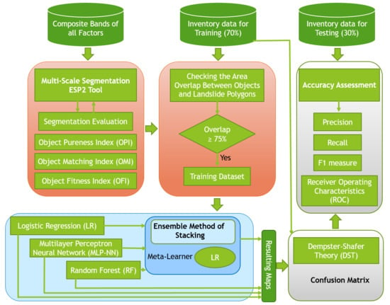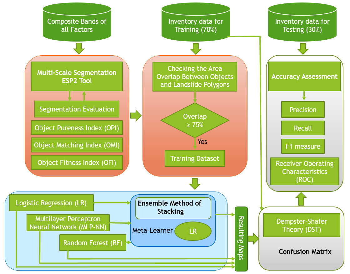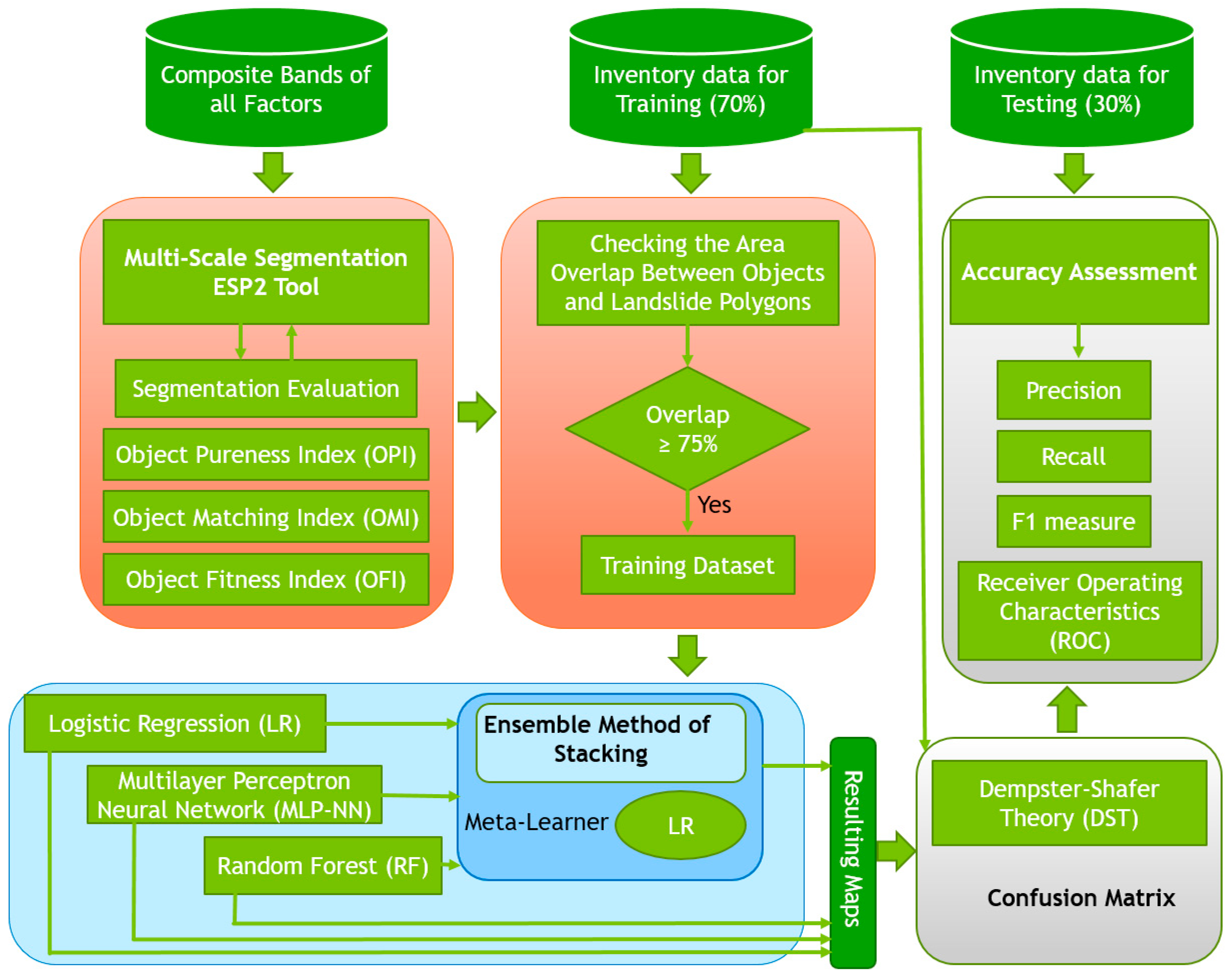[12] used the DST to enhance the results of the integration of OBIA with various ML methods, including SVM, random forest (RF), and K-nearest neighbor (KNN). The DST method performed well in landslide detection in their tropical study area. These pieces of evidence from previously published papers motivated us to apply the DST probability concept to improve the ML classification accuracy through integration with different classifiers. Therefore, in the present study, we integrate the widely used ML methods of logistic regression (LR), the multilayer perceptron neural network (MLP-NN), and RF with OBIA for landslide detection, based on optical data and topographic factors resulting from PlanetScope satellite images and Digital Elevation Model (DEM) data, respectively. To improve the performance of the applied ML methods, the ensemble method of stacking is used to combine them and produce a new result. The optimal scale for image segmentation is derived using the estimation of scale parameters (ESP2) tool [23]. Multiple scales are selected using interval values based on the optimal scale. The maps resulting from the multi-scale segmentation by each ML method are then fused using DST to demonstrate the advantages of working in a multi-scale environment. All resulting landslide detection maps are then validated using standard RS accuracy metrics and the validation method of receiver operating characteristics (ROC).

2. Study Area

In April 2015, an earthquake with a magnitude of 7.8 M struck Nepal, killing almost 9000 people and injuring nearly 22,000 [36]. The epicenter of the earthquake was located in the east of Gorkha district, and its hypocenter was at a depth of nearly 8.2 km [37]. Due to the magnitude of the earthquake, several landslides occurred across Nepal, especially in the east of the Gorkha district.

The study area of this research is located in the southern part of Rasuwa district (see Figure 1), along the Trishuli river. The study area covers around 17,100 ha, and the elevation ranges between 700 and 2038 m above the mean sea level (MSL). The land use largely consists of forested areas, grassland, agricultural land, and rural areas. The study area is located in the higher Himalayas and, due to its rough terrain, is very susceptible to landslide occurrence. According to the Köppen climate classification scheme, the study area falls under a sub-tropical and humid climate with cooler temperatures, and its annual average precipitation is nearly 691 mm. Before this study, some investigations by [38,39,40] and [1] were carried out to extract landslide locations in Rasuwa district. However, the main focus of the present study is evaluating the accuracy and performance of the proposed method of landslide detection compared to the conventional ML methods.

3. Methodology and Data

3.1. Overall Workflow

In this study, we used PlanetScope multispectral images [41] in four bands (Blue, Green, Red, and NIR), along with topographic factors, for landslide detection. The overall workflow (see Figure 2) of this study is as follows:

• Preparing multispectral images, the spectral index, and topographic derivatives for modeling;
• Generating multi-scale segments using the ESP2 tool and scale value intervals;
• Segmentation analysis and evaluation;
• Training ML and stacking methods on multi-scale datasets at the object level;
• Fusing multi-scale ML results using DST;
• Applying different accuracy assessment metrics.

3.2. Datasets

One of the most critical datasets for landslide detection and prediction is an appropriate landslide inventory, which influences further analyses [42,43]. In this case study, a landslide inventory map for the Rasuwa district was obtained from multiple sources, including GPS data from an extensive field survey and manually extracted data from satellite imagery. The satellite images used in this study were taken from the PlanetScope constellation of Planet Labs Company. PlanetScope includes more than 120 satellites that have been operating since 2014 and provide multispectral images with a 3 m spatial resolution and daily revisit time in four bands (

Table 1. PlanetScope satellite sensor specifications.

Satellite (Sensor)	Bands Wavelength (nm)				Pixel Size	Bit Depth	Orbit Altitude	Scene Size (KM)
PlanetScope	Blue	Green	Red	NIR	3.125 m	16	475 km	24.6 × 16.4
	455–515	500–590	590–670	780–860

). Due to the rugged topography of the study area, some landslide events could not be registered by the field survey, so satellite images were used to identify and digitize them. Subsequently, all types of data were converted to the polygon format in QGIS 3.8. The total number and area of landslide events that were mapped were 194 and 64120 ha, respectively. Moreover, the minimum, maximum, and standard deviation of the area of the landslide polygons were 0.07, 16, and 2.17 ha, respectively. Along with PlanetScope images (Table 1), the normalized difference vegetation index (NDVI) index—which is widely applied in landslide modeling [1,7,44]—was calculated from the NIR and Red bands to be used in landslide detection. The probability of landslide occurrence is highly dependent on the surface topography; in other words, hilly and mountainous areas have the highest probability of landslide occurrence [1]. Our study area is located within the Himalayan fold and thrust zone of central Nepal. This zone resulted from a collision of the Indian Plate with the Eurasian plate. The precipitation amount of this area varies based on the tropical climatic conditions in the monsoon season, which has more rainfall compared to the summer season [45]. Although geological formations and precipitation are also important for landslide modeling, these factors do not change significantly in this study area due to its small size, which is why they were not considered in this study. Therefore, only satellite images and topographic factors were used, and all topographic derivatives, such as elevation, slope, aspect, curvature, and the topographic wetness index (TWI), were calculated based on a 5 m resolution DEM. The selection of topographical factors related to landslide occurrences depends on the landslide type, characteristics of the study area, and scale of the analysis. However, there is no standard approach for the selection of landslide conditioning factors. In the present study, six topographical landslide conditioning factors, namely, slope, slope aspect, curvature, plan and profile curvature, and altitude, were generated from a 5 m resolution DEM acquired from the Japanese aerospace exploration agency JAXA ALOS sensor.

One of the most critical factors controlling slope stability is the slope angle. The slope angle is regularly used in landslide detection and susceptibility studies [46]. In the study area, the slope map was prepared using a DEM, and the slope ranged from 0.05° to 75.26°. The slope aspect was considered a topographical conditioning factor representing the slope direction [47]. The slope aspect factor mainly affects the hydrological system through evapotranspiration and, consequently, affects vegetation. Our aspect layer was classified, as this layer comprised sharp differences and changes. As such, the slope aspect of the area was divided into nine classes, namely, north, northwest, northeast, east, south, southeast, southwest, west, and flat.

We extracted the plane curvature from the DEM. The plane curvature represents the curvature of the contour line formed by the intersection of the surface with the horizontal plane [48]. The convergence and divergence of water in downhill flow are influenced by plane curvature [49]. The plane curvature represents the rate of change of aspect, in which positive values indicate convex curvature, zero denotes low change, and negative values indicate concave curvature. The values range from −56 to 74.14. The profile curvature is also crucial for the water flow speed variation from higher to lower areas [7]. The conditioning factor of altitude is another instability factor in our region, and landslide events at higher altitudes are usually influenced by gravity. Altitude influences topographical attributes and the Earth’s surface, which accounts for spatial variability in precipitation, soil thickness, erosion, and vegetation types [50]. In this study area, the elevation ranges from 734 to 4050 m above the mean sea level.

The landslide areas are usually not vegetated, especially due to recent landslide events [7]. Therefore, we used the normalized difference vegetation index (NDVI) to better distinguish between landslide and non-landslide areas. This index is useful for our study area, which is covered by forest. In this study, the NDVI map was derived from PlanetScope imagery from 28 November 2015 (see Equation (1)).

$$\mathrm{NDVI}=\frac{(NIR-\mathrm{Re}d)}{(NIR+\mathrm{Re}d)}$$

(1)

The NDVI was calculated from the near-infrared and the red spectral bands. The NDVI values vary from −0.44 to 0.72 in the study area.

The TWI is another important topographical conditioning factor within the morphometric conditions of the terrain, as it evaluates the cumulative flow rate upstream with the slope angle [51]. The TWI is calculated by Equation (2):

TWI = ln (α/tan β)

(2)

where α is the specific catchment area (m) and β is the slope. All conditioning factors are represented in Figure 3.

3.3. Object-Based Image Analysis (OBIA)

3.3.1. Multi-Scale Image Segmentation

The demand for high-resolution (HR) and VHR satellite imagery, together with the resulting volume, variety, and velocity, as well as the rapid development and progress of EO technologies, provide significant challenges for the RS community with respect to the complexity of image understanding (IU) [52]. Therefore, OBIA, as an almost new paradigm in EO data analysis and image processing, has attracted more and more attention in the RS community and has been applied in several applications, such as image classification and object extraction [17]. OBIA is a knowledge-driven approach that aims to produce meaningful objects by using geometric and spectral characteristics, such as size, shape, texture, color, and contextual information, to present a better IU based on the real world [13]. In OBIA, segmentation is a crucial step [53], which considerably influences further analyses and results. The way that segmentation parameters (e.g., scale, shape, and compactness) are selected impacts the quality of the image objects [54]. In this study, multiresolution segmentation (MRS) was applied for the segmentation of our PlanetScope image (see Figure 4). MRS is a bottom-up segmentation technique, which is based on the pairwise region-merging approach [12]. In this case, smaller detected objects were merged with larger ones, considering various parameters of scale, color, and shape (i.e., compactness and smoothness). These parameters are usually selected by trial-and-error, which requires expert knowledge and is a time-consuming and uncertain task [12,55]. Although some automatic techniques, like the Taguchi optimization method [55], have been introduced for defining the optimal parameters for the segmentation process, the process of detecting optimal objects is still a challenging task, mostly because of the diversity in the sizes and shapes of the target features [56].

The SP is considered the most crucial parameter in the MRS. In this study, the optimal SP was derived using the ESP2 tool, developed by [23]. This automated tool is a technique for selecting the SPs, which delivers three distinct scales using MRS, implemented in the eCognition Developer software. The ESP2 tool resulted in SP values at three different scale levels which, for our case, were 112 for scale level 1, 242 for scale level 2, and 1142 for scale level 3. The optimal SP value of the second level was selected along with two other scales based on an interval of 50 for further analysis and landslide detection. In pixel-based image classification, thematic accuracy assessment is the conventional method applied to evaluate the performance of an image classifier and the accuracy of a produced map [57], based on the proportion of correctly and incorrectly classified pixels, which is a count-based classification accuracy index [21]. In OBIA, on the other hand, processing units are image objects, which are two-dimensional polygon features. Therefore, it is necessary to evaluate these objects with reference objects to assess the performance of the applied segmentation method [22]. In this regard, a variety of indices and metrics have been proposed, which are either area-based or location-based [22]. The accuracy of the segmentation using the selected scales was evaluated and presented in Section 3.3.2.

3.3.2. Segmentation Accuracy Evaluation

Although we used the ESP2 tool to determine the optimal SP, there is no standard method to select segmentation parameters or assess the accuracy of the resulting objects [22]. The segmentation parameters are usually modified based on the desired target features, and they are challenging to implement and cannot appropriately address errors like under- and over-segmentation [22]. Therefore, we applied two indices that enabled us to evaluate the resulting objects using the multiresolution segmentation technique, along with the ESP2 tool and the corresponding interval values. These indices were the Object Pureness Index (OPI) on the one hand, and the Object Matching Index (OMI) on the other hand. OPI is a measure used to assess the integrity of the object in terms of spectral characteristics, and it is based on the standard deviation (SD) of multispectral bands because there is a robust positive correlation between the applied bands. The reason that SD is selected instead of each band’s mean value is that mean values vary among these bands, while SD values are very close to each other, especially for integrated objects like vegetated areas and water bodies. The other considered measure, OMI, evaluates the spatial match between the reference object and the image objects. The mathematical explanation of these measures is stated in Equation (3):

$$\mathrm{OPI}=\frac{\frac{{(\mathrm{SD}}_{\mathrm{B}}{+\mathrm{SD}}_{\mathrm{G}}{+\mathrm{SD}}_{\mathrm{R}})}{3}}{\mathrm{Max}\mathrm{SD}}=\frac{{(\mathrm{SD}}_{\mathrm{B}}{+\mathrm{SD}}_{\mathrm{G}}{+\mathrm{SD}}_{\mathrm{R}})}{3\ast \mathrm{Max}\mathrm{SD}}$$

(3)

where SD_B, SD_G, and SD_R stand for the SD of the Blue, Green, and Red bands, respectively, and Max SD stands for the maximum SD value among these three bands. The OPI values close to 1 indicate that spectral variance is very low and the object is pure. In comparison, OPI values close to zero indicate that there is significant variance among the resulting objects, which usually happens when large-scale values are applied in the segmentation process. OPI alone is not adequate for selecting segmentation parameters, because it only evaluates objects in terms of spectral features, and does not address the spatial matching of objects. Therefore, the OMI (see Equation (4)) was also applied to evaluate our segmentation:

$$\mathrm{OMI}=\frac{\mathrm{Area}(\mathrm{R}\cap \mathrm{S})}{\mathrm{Area}\left(\mathrm{R}\right)}\times \frac{\mathrm{Area}\left(\mathrm{S}\right)}{\mathrm{Area}\left(\mathrm{R}\right)}$$

(4)

where R is a reference object and S is a segmented object. An OMI value equal to 1 shows a perfect match between R and S, while values less than 1 indicate over-segmentation and values greater than 1 indicate under-segmentation. The Object Fitness Index (OFI) is calculated (as per Equation (5)) to obtain a single index that can present the optimal object generation scale based on OPI and OMI, among other scales:

$$\mathrm{OFI}=\sqrt{(\frac{{\mathrm{OPI}}^2{+\mathrm{OMI}}^2}{2}})$$

(5)

OFI values close to 1 point to the optimal segmentation scale. Resulting values less and greater than 1 indicate over- and under-segmentation, respectively.

3.4. Machine Learning Methods

3.4.1. Multilayer Perceptron Neural Network (MLP-NN)

ML algorithms have been widely used in various scientific fields, especially in the earth sciences, to overcome complex problems [58,59]. ML is considered a subdivision of artificial intelligence, which imitates the human brain’s performance in problem-solving and decision making [60]. In doing so, it uses a variety of algorithms, like artificial neural network (ANN), in the learning process [59]. MLP-NN is an ANN method that has been widely used in geohazard modeling [1]. The performance of this method is affected by variables like the model’s structure, the type of applied activation functions, and which weight updating method is used [61]. In general, MLP-NN consists of an input layer, one or more hidden layers, and an output layer. In geohazard modeling, like landslide susceptibility modeling, the input layer includes neurons that are the same as the landslide affecting factors, and the number of hidden layers depends on the training data [62] and the complexity of the problem [1]. In this study, the backpropagation algorithm (BPA), which is the primary training method employed in neural networks, was used for updating weights; for two hidden layers, 24 neurons for each layer were allocated. To run the method, initial weights, which are randomly chosen by the BPA, are allocated to each neuron, and the method is then continually optimized based on the error rate between the output and expected values until the error rate is stabilized (see Equation (6)):

$$y=({\displaystyle \sum _{i=1}^n{W}_i}\ast X_i+b)$$

(6)

where W denotes the vector of weights, X is the input vector of features of objects, and b is the bias. Additionally, the sigmoid activation function, which was used in the present study, can be explained by Equation (7):

$$f \left(\mathrm{z}\right)=\frac{1}{1-e^{-y}},$$

(7)

where f (z) is the output of the activation function, which ranges from 0 to 1.

3.4.2. Logistic Regression (LR)

Logistic regression is one of the multivariate analysis methods that allow us to create a multivariate regression connection among a set of independent variables and one dependent variable [63]. LR is a powerful method for predicting the presence of an event by fitting the best linear model based on independent variable values, and it is a commonly used statistical method applied in landslide susceptibly analysis [64]. One of the significant advantages of LR is that, in this method, the independent variables can be both discrete and continuous, or a mix of these variable types can be used [65]. In this case, the dependent variable was introduced as a binary value of 0 and 1, whereby 0 showed the absence of a landslide event and 1 indicated the presence of a landslide. The mathematical definition of LR is defined by Equation (8) [63]:

$$\mathrm{p}=\frac{1}{(1+e^{-\mathrm{z}})}$$

(8)

where p, in this case, is the probability of a landslide occurring, which varies between 0 and 1. Furthermore, z is the linear combination, which fits a linear equation to independent variables (landside conditioning factors), as shown by Equation (9) [63]:

$${z=b}_0{+b}_1{x}_1{+b}_2{x}_2{+b}_3{x}_3+\dots {+b}_n{x}_n$$

(9)

where b₀, b_i, and x_i are intercepts of the method, coefficient, and independent variables, respectively.

3.4.3. Random Forest (RF)

RF is a powerful supervised ML method, which was proposed by [66] and has been widely used in RS and GIS applications, such as image classification [67] and landslide susceptibility mapping [1]. This method is based on decision trees and operates by constructing a multitude of decision trees during the training process, which makes it less sensitive to over-fitting issues [1]. In the RF method, each decision tree generates outputs, and then outputs weights, which are derived from the votes, are dedicated. The advantages of RF are that it is easy to apply because it requires fewer parameters and it yields a higher accuracy compared to other ML methods due to the bagging process [68]. Additionally, it can deal with high-dimensional and complex data structures [69]. Due to its simplicity and better performance, we selected this method as another algorithm for landslide detection in this study.

3.4.4. Stacking Machine Learning (ML) Methods

The main idea behind ensemble methods in ML is to improve the performance of a final method, by combining various methods to build a powerful learner to predict or classify a set of data [70]. The strength of using ensemble methods is that we can decrease the variance by combining several single methods, which, individually, do not yield an excellent performance [70]. There are three main ensemble machine learning methods: bagging, boosting, and stacking. In this case, the stacking method was used. In stacking, there are two levels, namely, level 0 and level 1. In level 0, single methods make a set of predictions based on training data, and these outputs (predictions) are then used as inputs for a meta-learner, which is a single method, to make a new set of predictions [71]. Therefore, in this case, ML methods such as LR, MLP-NN, and RF were trained as single methods in level 0, and LR was then used as our meta-learner in level 1 to make the final predictions.

3.5. Integration of MLP-NN and OBIA for Landslide Detection

In conventional landslide detection and susceptibility mapping using machine learning algorithms, analyses are usually performed on an n-dimensional raster dataset or, to be specific, calculations are at the pixel level, and the pixel values in each layer are processed. Applying ML algorithms to large or very high-resolution datasets at a pixel level requires robust computing systems and is time-consuming, in particular, when the spatial extent of the study area is significant. Meanwhile, in OBIA, analyses are carried out at an object level [53], and processes like classification are relatively fast compared to pixel-based methods because, instead of processing each pixel in a set that shares the same values, the mean value of the object that entails a set of similar pixels will be analysed. In addition to the mean values of objects in each layer (e.g., image bands, DEM, NDVI, etc...), other statistical and geometrical characteristics, such as the SD, mode, shape index, position, and texture, can be calculated and used in classification and feature extraction [53]. Therefore, in this integrated approach, we first produced image objects through a multiresolution segmentation process by using different scale factors and then calculated the statistical and geometrical properties for each object. To train ML methods, objects that had more than a 75% overlapping area with training inventory polygons were selected as the training dataset. Finally, the methods were trained and applied on test data, which were converted to a comma-separated values (CSV) format in Python using sklearn’s ML package.

3.6. Dempster–Shafer Theory (DST)

The concept of DST is made based on a frame of discernment and known as a belief function (Bel) that is derived from Bayesian probability theory (BPT). It obtained its name from the extensions and clarifications presented by Shafer and is considered a great approach to integrating spatial data [72]. The DST is an effective method for modeling imprecision and uncertainty assessment. The DST is transformed from events to proposition and an event set to proposition set, which defines the concept of the basic probability assignments (bpa) function, Bel, and the plausibility function (Pl), and determines the one-to-one relationship of proposition and set. Therefore, the DST can translate the proposition uncertainty into a set uncertainty [73]. In this theory, displaying information requires two essential functions, namely, Bel and the Pl, which derive the lower bound value for a known probability function and the upper bound value for an unknown probability function. The differentiation between Bel and Pl illustrates the uncertainty of the knowledge about the objective proposition.

The DST provides an extension of the probability framework for assessing the uncertainty of any imprecision event of the probability P(M_l) that the alternative method M_l, l = 1, ..., n is correct. The lower bound indicates the degree of knowledge or belief that supports M_l and represents Bel (M_l). In comparison, the upper bound indicates the probability of M_l, and is called plausibility Pl (M_l) [74] (see the Equations (10) and (11)):

$$Bel \left(A\right)={\displaystyle \sum }_{B\subseteq A}m\left(B\right)$$

(10)

$$Pl \left(A\right)={\displaystyle \sum }_{B{{\displaystyle \cap }}^{\text{}}A\ne 0}m\left(B\right)$$

(11)

where the summation is obtained over all sets B$\in 2$^ɵ with B$\subseteq A$ in the definition of Bel and the summation in that of Pl is taken over all B$\in 2$^ɵ with B${{\displaystyle \cap }}^{\text{}}A\ne 0$ in which the set of ɵ is mutually exclusive and collectively exhaustive hypotheses, and the power set of ɵ is denoted by 2^ɵ. The Bel is the summation of all masses directly assigned by a set of hypothesis A, while the plausibility sums all masses not assigned to the complement of the hypothesis A. An uncertainty interval of $\lfloor Bel\left(A\right),Pl\left(A\right)\rfloor$ that Bel (A) ≤ Pl(A) can be defined; its length is a measure of the imprecision of knowledge about the uncertainty of set A [75].

From a general point of view, unlike a probabilistic theory that allocates a mass to the individual elementary events, the theory of evidence, or the bpa, makes m(A) on the set A of the P(z), power sets of the space Z event, i.e., on a set of results rather than a single elementary event.

In more detail, m(A) expresses the degree of belief that a specific element x belongs to the set A only, and not to any subset of A. The bpa that assigns a mass in the range of [0, 1] to each subset A satisfies the following requirement, specified by Equation (12):

$$\mathrm{m}:P\left(z\right)\to \left[0,1\right],\mathrm{m}\left(\mathsf{\phi }\right)=0;{\sum }_{A\in Z}m\left(A\right)=1$$

(12)

If n data sources are available, probability masses m_i (B_j) must be defined for each data source i with 1 ≤ i ≤ n and for all sets, B_j $\in$ 2^ɵ. The DST allows the combination of these probability masses from resulting landslide detection maps and the training inventory data set to compute a combined probability mass for each set. The composition rule in the proposed DST is based on mathematical theory, which is the basis of the combination of mass functions m_i obtained from n sources of information given in Equations (13) and (14):

$$m\left(A\right)=m_1\left(B_1\right)\oplus m_2 \left(B_2\right)\oplus M_3\left(B_3\right).\dots \oplus m_n\left(B_n\right)$$

(13)

$$m\left(A\right)=\frac{{{\displaystyle \sum }}_{B_1{{\displaystyle \cap }}^{\text{}}{B}_2\dots .B_n=A }{{\displaystyle \prod }}_{i=1}^n{m}_i\left(B_j\right)}{\left(1-K\right)}$$

(14)

where K denotes the degree of conflict given in Equation (15):

$$K={\sum }_{B_1{{\displaystyle \cap }}^{\text{}}{B}_2\dots .B_n=\mathsf{\phi }}{{\displaystyle \prod }}_{i=1}^n{m}_i\left(B_j\right)$$

(15)

Fusion of Multi-Scale Results via DST

Multi-scale segmentation resulted in different object sizes, which were used for training the ML methods. Therefore, based on multi-scale segmentation, different landslide detection maps were produced from each ML method. The areas that were classified as landslides using different scales and one ML method were grouped by the fusion level analysis (FLA) technique [12] and fused into a class of landslide area based on the DST. Several Bels were combined in the DST within the same frame, which made it possible to harmonize the landslide detected areas from different scales. The probability of uncertainty in the detected landslide areas can be derived from Bel and Pl. Therefore, the resulting areas detected as landslides in three scales (i.e., 198, 248, and 298) were combined by fusing the DST with the training inventory dataset. The accuracy of the landslide detected areas based on each scale was assessed using a confusion matrix and, accordingly, the Bels were estimated by a precision function [12]. The DST combined the majority of landslide detected areas, which were closer to the inventory dataset, and then assigned them to the class of landslide area based on the DST.

4. Accuracy Assessment and Comparison

In this section, we outline the most common accuracy assessment methods, which were used to validate the performance of the applied ML methods and the improvements made by using the stacking and DST methods. The accuracy assessment was made by comparing the resulting landslide detection maps with the landslide inventory dataset. The accuracy assessment was conducted using a confusion matrix, precision, recall F1 measure, and the receiver operating characteristics (ROC), to determine the accuracy of the landslides detected by each method. The user accuracy was calculated based on dividing correctly mapped objects by the total number of classified objects. In this regard, the study area was divided into two classes called landslide areas and non-landside areas, and for each class, this measure was calculated. We used the confusion matrix based on a comparison of the inventory dataset and the resulting maps based on a pixel-based environment. The Kappa coefficient was derived from the confusion matrix [76], and the coefficient was calculated using Equation (16):

$$\mathrm{Kappa}\mathrm{Coefficient}=({\theta }_1- {\theta }_2) /\left(1- {\theta }_2\right)$$

(16)

where ${\theta }_1$ denotes the ratio of correctly detected areas, whereas ${\theta }_2$ denotes the proportion of agreement by randomness [12].

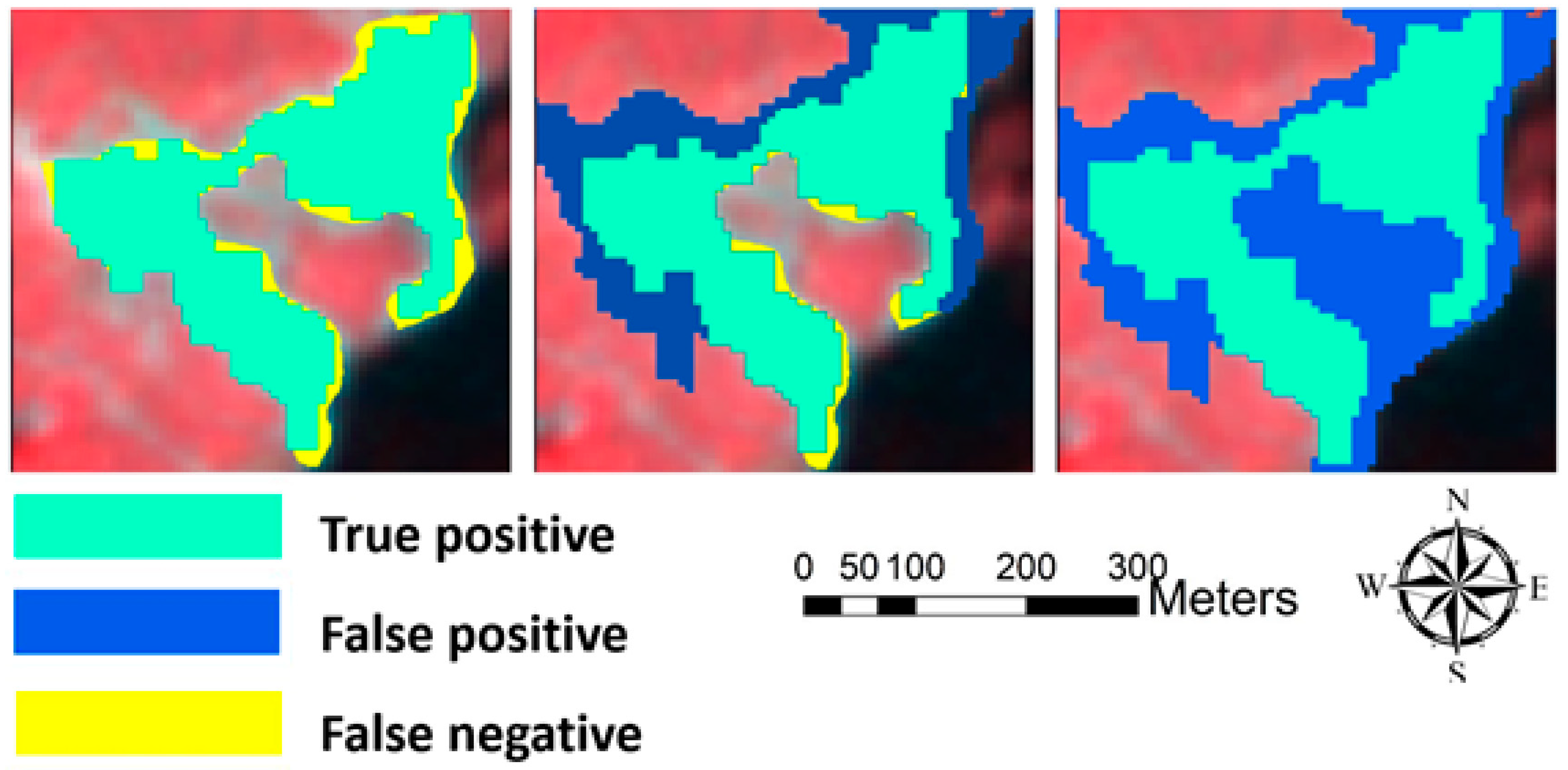
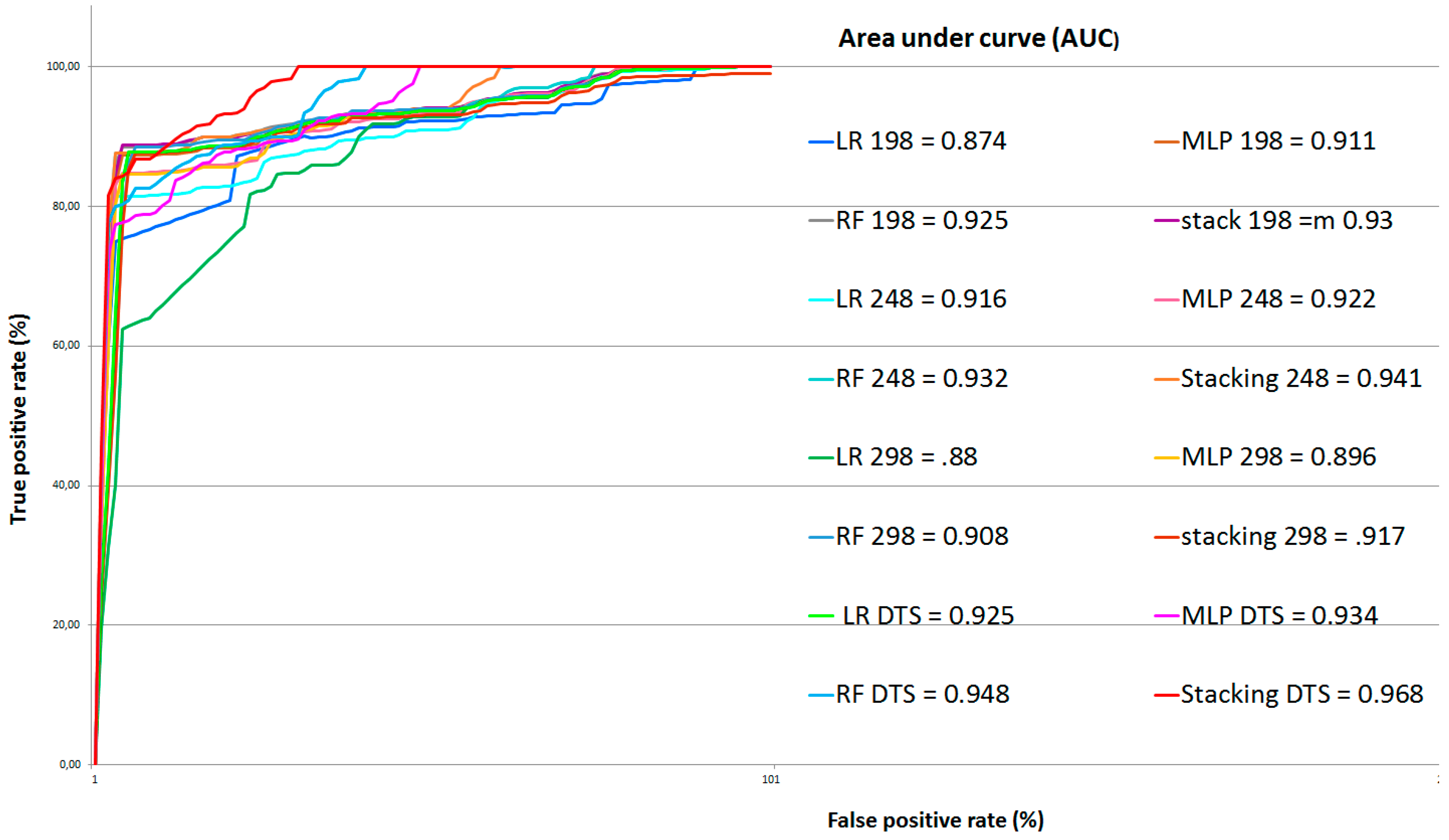
The ROC is a graphical plot used to evaluate the validity of a method that predicts the location of the occurrence of events by comparing the probabilistic map of the event with a reference map [77]. This assessment method has been applied in many fields, in particular, in the Geosciences [78]. 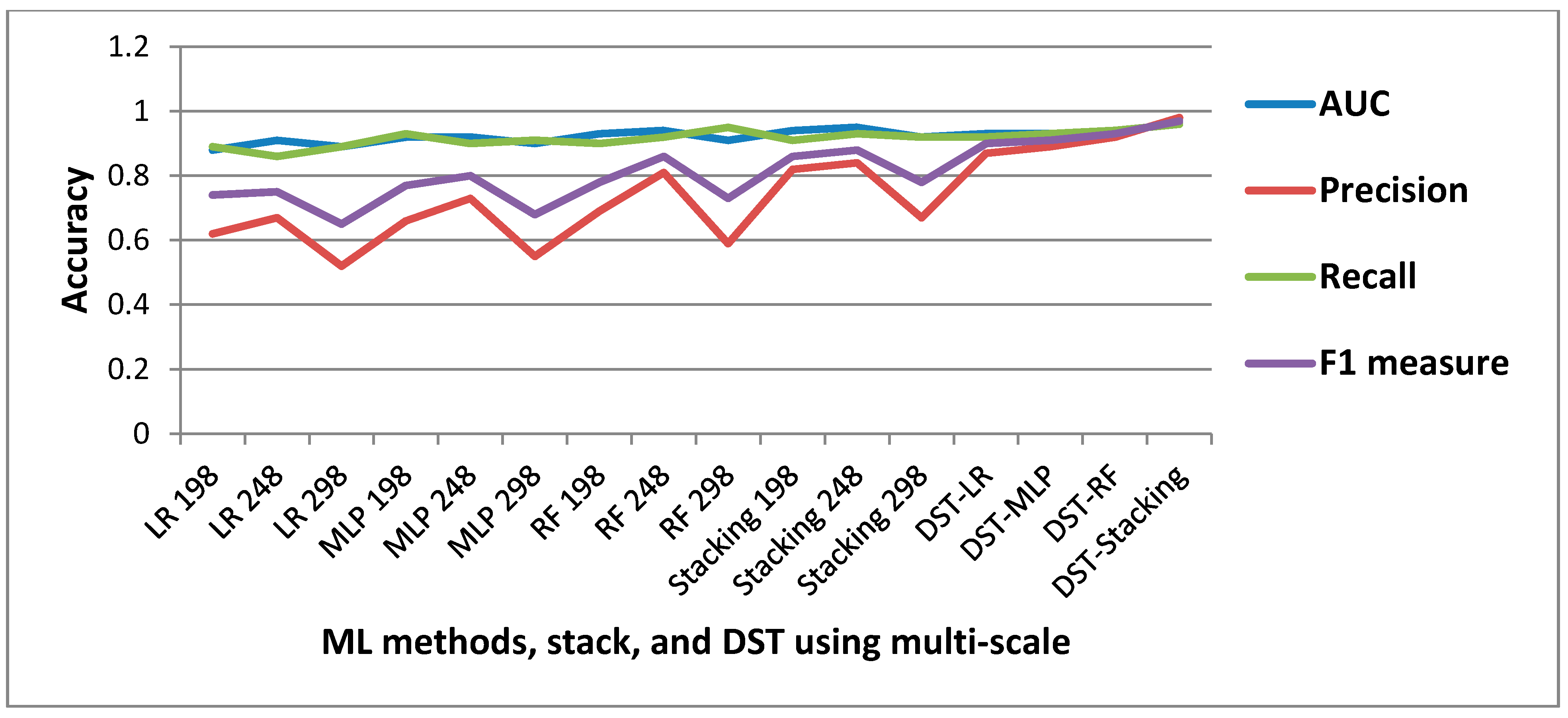The ROC measure is based on three metrics: true positive (TP), false positive (FP), and false-negative (FN) (see Figure 5 and Equations (17)–(19)). In this case, the landslide events that were correctly detected were TPs, areas that were incorrectly classified as landslides were FPs, and FNs represented landslide areas that were not detected. Using these metrics, the three parameters of Precision, Recall, and F1 measure could be calculated to assess the results. Precision shows the proportion of landslide events that were detected, Recall indicates how many of the inventory landslide events were detected, and the F1 measure was used to balance the Precision and Recall.

$$\mathrm{Precision}=\frac{{\mathrm{TP}}_{\mathrm{s}}}{{\mathrm{TP}}_{\mathrm{s}}{+\mathrm{FP}}_{\mathrm{s}}}$$

(17)

$$\mathrm{Recall}=\frac{{\mathrm{TP}}_{\mathrm{s}}}{{\mathrm{TP}}_{\mathrm{s}}{+\mathrm{FN}}_{\mathrm{s}}}$$

(18)

$$\mathrm{F}1\mathrm{meausre}=2\times \frac{\mathrm{Precision}\times \mathrm{Recall}}{\mathrm{Precision}+\mathrm{Recall}}$$

(19)

5. Results and Discussion

5.1. Image Segmentation

The MRS parameters and results of ten applied scales were chosen by interval values based on the ESP2 tool scale value of 248. The NDVI and topographic derivatives, along with PlanetScope images, were used as the conditioning factors in our image segmentation procedure, to improve the segmentation results. Next, to evaluate the accuracy of our segmentation results, 30% of the inventory dataset of landslide events were randomly selected for use in the OPI, OFI, and OMI indices. The applied parameters and layer weights, and the segmentation evaluation results are presented in

Table 2. Parameters used for the multiresolution segmentation (MRS) and segmentation evaluation results.

Scale	Shape	Compactness	Layer Weights									OPI	OMI	OFI
			RGB NIR	TWI	Aspect	Profile Curvature	Elevation	NDVI	Slope	Curvature	Plan Curvature
48	0.7	0.3										0.88	0.40	0.68
98	0.7	0.3										0.93	0.51	0.75
148	0.7	0.3										0.95	0.71	0.84
198	0.7	0.3										0.95	0.87	0.91
248	0.7	0.3	2	1	2	1	1	4	2	1	1	0.97	0.95	0.96
298	0.7	0.3										0.94	1.19	1.07
348	0.7	0.3										0.92	1.25	1.10
398	0.7	0.3										0.90	1.29	1.11
448	0.7	0.3										0.87	1.35	1.14
498	0.7	0.3										0.81	1.41	1.15

.

For the accuracy assessment of our segmentation results, we selected image objects whose centroids were within the reference objects. According to Table 2, based on the OFI index results of 30% of the applied samples, the segmentation with a scale of 248 provides the best convergence, while scales lower and higher than scale 248 are associated with over-segmentation and under-segmentation errors, respectively. The variation of the resulting values from OPI, OMI, and OFI are shown in Figure 6. The segmentation results in Figure 7 show the over- and under-segmentation errors. In Figure 7a, due to a small SP, the landslide event is over-segmented, while in Figure 7c, the scale is relatively large, resulting in under-segmentation, which merged a non-landslide area with a landslide area. Figure 7b shows the best segmentation result compared to other scales. The main reason that three scale results are used for landslide detection is to evaluate the impact of different scales on the landslide detection accuracy. Since, in OBIA, processing units are image objects, other features (e.g., geometric, textural, and spectral) of objects can be calculated and used in the classification or object extraction. Therefore, in this case, we calculated characteristics such as the shape index, mean brightness, SD of NDVI, length, compactness, density, and contrast grey level of the co-occurrence matrix (GLCM), to be used in MLP-NN algorithms. In order to train MLP-NN for each segmentation result, the objects that overlapped with training data (polygons) were chosen as training objects. Subsequently, the trained algorithm was applied to test objects.

5.2. Landslide Detection using ML and Stacking Methods

The training image objects of each segmentation scale, along with their characteristics, were stored in a CSV file to train ML methods in the Python environment. Results for all scales vary between 0 and 1, and objects that had values greater than 0.5 were selected as landslide events for all ML methods. The results in Figure 8 show that the size of objects has a significant impact on the outputs. For example, the results of ML and stacking methods of image objects with a scale of 298 indicate larger areas as landslides than the other scales’ results. However, based on the OPI and OMI indices, differences in the results were expected, because the OPI and OMI values of scales 198 and 248 are close to each other and are associated with an over-segmentation error. Meanwhile, for the scale 298, the values of those indices—OMI, in particular—show an under-segmentation error, which resulted in larger image objects. Additionally, the methods’ parameters were the same for each segmentation scale.

5.3. Results of Fusion and Optimization using DST

To optimize the landslide detection using the ML method and obtain the best result, we used DST to combine the results of each method’s landslide detection output at different scales. Therefore, the predicted landslides acquired from each method were calculated using a confusion matrix, and a CSV file was employed to fuse the most probable landslide events in QGIS 3.8, which resulted in a single and accurate landslide inventory map for each method (Figure 8).

According to the results, which are represented in

Table 3. Confusion matrices based on different methods and the landslide inventory data set.

Method	Class Name	Pixels from Landslide Inventory Data Set		Total Samples	User Accuracy	Overall Accuracy	Kappa Index
		Non-Landslides	Landslides
LR 198	Non-landslides	1755	370	2125	82,588	0.761	0.541
	Landslides	400	700	1100	63,636
MLP 198	Non-landslides	1774	351	2125	83,482	0.769	0.555
	Landslides	395	705	1100	64,091
RF 198	Non-landslides	1786	339	2125	84,047	0.774	0.566
	Landslides	389	711	1100	64,636
Stacking 198	Non-landslides	1779	346	2125	83,718	0.778	0.576
	Landslides	371	729	1100	66,273
LR 248	Non-landslides	1874	251	2125	88,188	0.833	0.685
	Landslides	289	811	1100	73,727
MLP 248	Non-landslides	1890	235	2125	88,941	0.841	0.700
	Landslides	279	821	1100	74,636
RF 248	Non-landslides	1914	211	2125	90,071	0.864	0.749
	Landslides	227	873	1100	79,364
Stacking 248	Non-landslides	1922	203	2125	90,447	0.872	0.765
	Landslides	209	891	1100	81,000
LR 298	Non-landslides	1744	381	2125	82,071	0.755	0.528
	Landslides	410	690	1100	62,727
MLP 298	Non-landslides	1769	356	2125	83,247	0.764	0.545
	Landslides	405	695	1100	63,182
RF 298	Non-landslides	1778	347	2125	83,671	0.769	0.554
	Landslides	399	701	1100	63,727
Stacking 298	Non-landslides	1779	346	2125	83,718	0.774	0.567
	Landslides	382	718	1100	65,273
LR DST	Non-landslides	1894	231	2125	89,129	0.861	0.745
	Landslides	217	883	1100	80,273
MLP DST	Non-landslides	1910	215	2125	89,882	0.870	0.762
	Landslides	206	904	1110	81,441
RF DST	Non-landslides	1970	155	2125	92,706	0.892	0.801
	Landslides	192	908	1100	82,545
Stacking DST	Non-landslides	1976	149	2125	92,988	0.898	0.814
	Landslides	180	930	1110	83,784

, the RF method achieved the highest user accuracy of all ML methods, with an accuracy of up to 90.07% when detecting non-landslides using the optimal SP. This resulting accuracy was followed by the MLP-NN and LR methods, with almost an 89% and 88.2% accuracy, respectively, again using the optimal SP. For this SP, the stacking method slightly improved the user accuracy to 90.44%. However, combining multi-scale results using the DST increased the user accuracy for all applied methods by up to 9%.

In the ROC analysis, the area under the curve (AUC) is a metric that evaluates each method’s performance in distinguishing between classes. In our case, these classes are landslide areas and non-landslide areas [79]. AUC values close to 1 indicate the reliability of a method’s results; however, values close to 0.5 show a method’s poor performance.

Table 4. Quantitative accuracy assessment for ML and Stacking methods, as well as DST results.

Method	Scale	TP (ha)	FP (ha)	FN (ha)	Precision	Recall	F1 Measure
LR	198	572.89	344.72	68.24	0.62	0.89	0.74
	248	553.39	272.62	87.74	0.67	0.86	0.75
	298	570.65	532.20	70.48	0.52	0.89	0.65
MLP	198	598.96	310.09	42.17	0.66	0.93	0.77
	248	580.04	220.00	61.09	0.73	0.90	0.80
	298	580.47	479.65	60.66	0.55	0.91	0.68
RF	198	579.54	265.76	61.59	0.69	0.90	0.78
	248	588.54	140.23	52.59	0.81	0.92	0.86
	298	608.44	419.65	32.69	0.59	0.95	0.73
Stacking	198	580.30	131.23	60.83	0.82	0.91	0.86
	248	594.25	109.23	46.88	0.84	0.93	0.88
	298	591.52	289.60	49.61	0.67	0.92	0.78
DST	LR	589.74	84.25	51.39	0.87	0.92	0.90
	MLP	594.36	74.44	46.77	0.89	0.93	0.91
	RF	604.15	55.85	36.98	0.92	0.94	0.93
	Stacking	616.06	11.93	25.07	0.98	0.96	0.97

presents the quantitative assessment accuracy of each method based on the testing inventory dataset. The ROC validation results showed that the DST-stacking results achieved the highest AUC value of 0.965, whereas the LR method, based on the scale of 180 with an AUC value of 0.88, presented the lowest accuracy in landslide detection (see Figure 9 and

Table 5. The accuracy assessment results based on the area under the curve (AUC).

Scale	LR	MLP	RF	Stack
198	0.88	0.92	0.93	0.94
248	0.91	0.92	0.94	0.95
298	0.89	0.9	0.91	0.92
DST	0.93	0.93	0.94	0.96

). Furthermore, for each result, the precision, recall, and F1 measures were also calculated.

To visually present the improvement of the results using the optimal scale, stacking, and DST, we enlarged a specific area of a landslide event (see Figure 10). This figure illustrates that the ML and stacking results based on objects at a scale of 298 are much more prone to FPs. Although the multi-scale approach resulted in different TP, FP, and FN areas, the DST was helpful for merging the TP areas of different scales and considerably improved the landslide detection accuracy. For instance, the result of stacking at a scale of 298 resulted in considerably more FPs, but this was not the case for the other scale levels, namely 248 and 198. However, as the DST combined the majority of TP areas, the FPs of the scale 298 were removed from the DST results.

The present study aimed to evaluate the performance of commonly used ML methods in landslide detection in an object-based environment. As shown in Figure 11, our validation results proved that all methods obtained the highest accuracy when using objects with a scale of 248, compared to lower and higher scales. However, applying the DST to combine the results of multiple scales for each method improved the overall accuracy of each method. Regarding the applied ML methods in this study, the stacking method yielded the highest accuracy at any scale compared to using single ML methods. The RF method performed best among the single ML methods, whereas the LR method achieved the lowest accuracies. Therefore, using the optimal SP and ML method is crucial for landslide detection in an object-based environment. We used the seismic-induced landslides as a case instant to evaluate the proposed methodology. However, this method can be applied for other types of landslides, and the outcome may depend on the resolution of the applied satellite imagery and the optimal scale parameter of segmentation. The limitation of this work is that the methodology is outperformed for a high-vegetated area, which was helpful to differentiate landslide areas from non-landslide ones. Therefore, it cannot reach the same accuracies for areas with less vegetation cover.

6. Conclusions

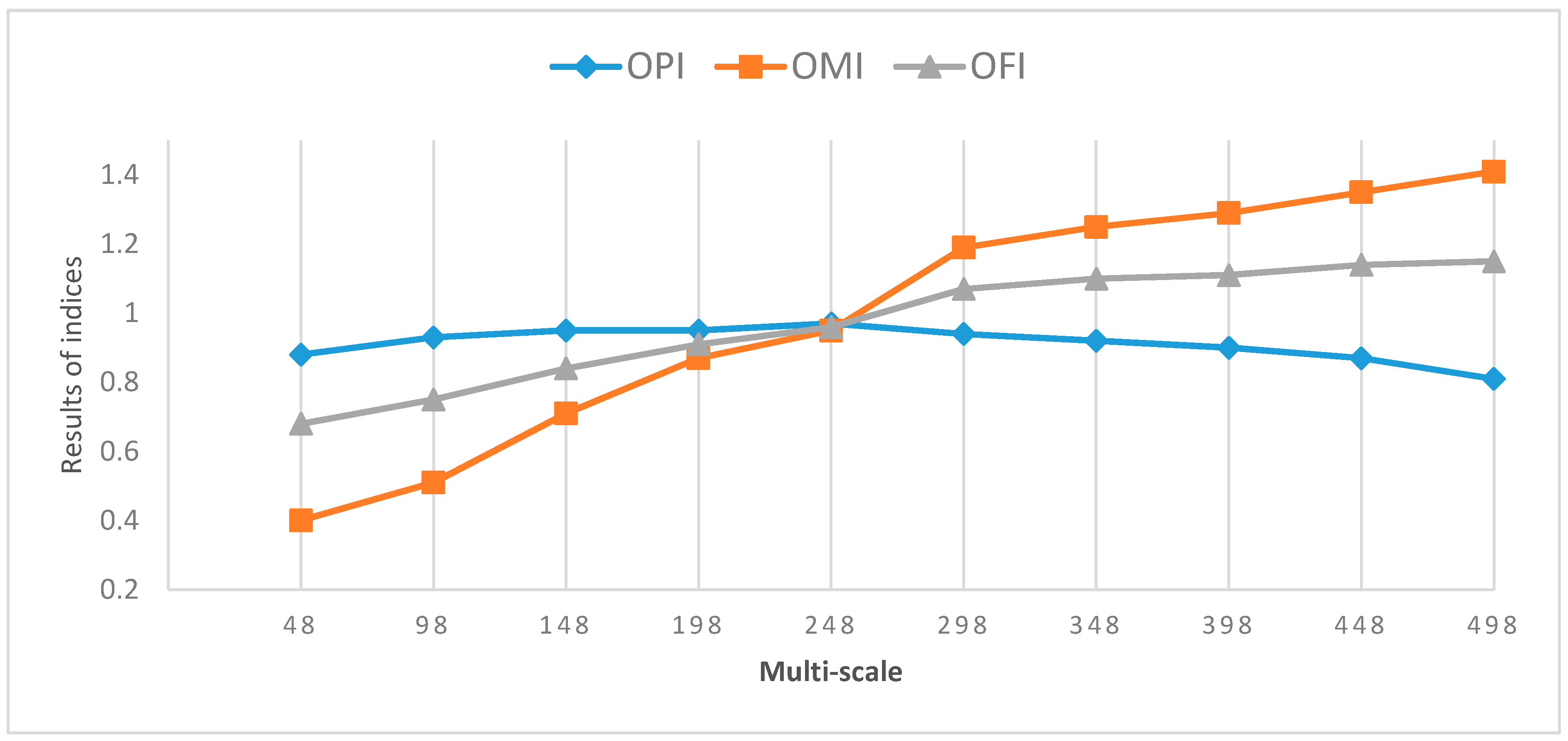
We have developed a methodology that incorporates OBIA with three machine learning methods, namely, logistic regression (LR), the multilayer perceptron neural network (MLP-NN), and random forest (RF), for landslide detection. Our multi-scale methodology identifies the optimal scale parameters (SP) and uses them for multi-scale segmentation and further analysis. The presented landslide mapping study showed that the integrated method improves the performance and accuracy. Most notably, the stacking method for landslide detection outperformed every single ML method. Furthermore, the validation results show that using DST could optimize and improve the outcomes of all applied methods. However, it should be noted that the results of an object-based ML method strongly depend on the segmentation quality. Therefore, optimal segmentation parameters result in a higher segmentation accuracy and, consequently, better results. Although there are no standard methods for selecting segmentation parameters and for accuracy assessment, we used the two measures of OPI and OMI to identify ideal segmentation parameters in terms of spectral and spatial quality. Therefore, as a result, both measures were combined to create the OFI, which allowed us to identify the best segmentation parameters, as well as to identify over-segmentation and under-segmentation errors. Therefore, we believe that a challenge for object-based ML methods is improving the segmentation accuracy, which requires new reliable automatic methods dealing with intra-class heterogeneity and inter-class homogeneity. This study shows that using high-resolution satellite imagery data does not guarantee a good accuracy. Several measures and parameters should be identified based on the target object detection or classification. In this regard, we used an ensemble method of stacking and DST to enhance the landslide detection results based on multi-scale segmentation. Different accuracy assessment results proved that the performance of landslide detection can be increased using these two methods. Moreover, all resulting maps yielded the highest accuracies using the optimal SP. Therefore, finding the optimal SP for the applied satellite image and ML method for the classification is crucial for accurate landslide detection. Based on the results of the present study, our future work will focus more on improving both segmentation and classification using relative mathematical and probability concepts, such as the central limit theorem (CLT) and fuzzy set theory (FST).

References

1. Ghorbanzadeh, O.; Blaschke, T.; Gholamnia, K.; Meena, S.R.; Tiede, D.; Aryal, J. Evaluation of Different Machine Learning Methods and Deep-Learning Convolutional Neural Networks for Landslide Detection. Remote Sens. 2019, 11, 196. [Google Scholar] [CrossRef]
2. Cruden, D.M. A simple definition of a landslide. Bull. Eng. Geol. Environ. 1991, 43, 27–29. [Google Scholar] [CrossRef]
3. Pawłuszek, K.; Marczak, S.; Borkowski, A.; Tarolli, P. Multi-Aspect Analysis of Object-Oriented Landslide Detection Based on an Extended Set of LiDAR-Derived Terrain Features. ISPRS Int. J. Geo-Inf. 2019, 8, 321. [Google Scholar]
4. Hong, H.; Chen, W.; Xu, C.; Youssef, A.M.; Pradhan, B.; Tien Bui, D. Rainfall-induced landslide susceptibility assessment at the Chongren area (China) using frequency ratio, certainty factor, and index of entropy. Geocarto Int. 2017, 32, 139–154. [Google Scholar] [CrossRef]
5. Pourghasemi, H.R.; Rahmati, O. Prediction of the landslide susceptibility: Which algorithm, which precision? Catena 2018, 162, 177–192. [Google Scholar] [CrossRef]
6. Guzzetti, F.; Mondini, A.C.; Cardinali, M.; Fiorucci, F.; Santangelo, M.; Chang, K.-T. Landslide inventory maps: New tools for an old problem. Earth-Sci. Rev. 2012, 112, 42–66. [Google Scholar] [CrossRef] [Green Version]
7. Pourghasemi, H.; Gayen, A.; Park, S.; Lee, C.-W.; Lee, S. Assessment of landslide-prone areas and their zonation using logistic regression, logitboost, and naïvebayes machine-learning algorithms. Sustainability 2018, 10, 3697. [Google Scholar] [CrossRef]
8. Goetz, J.; Brenning, A.; Petschko, H.; Leopold, P. Evaluating machine learning and statistical prediction techniques for landslide susceptibility modeling. Comput. Geosci. 2015, 81, 1–11. [Google Scholar] [CrossRef]
9. Feizizadeh, B.; Blaschke, T.; Tiede, D.; Moghaddam, M.H.R. Evaluating fuzzy operators of an object-based image analysis for detecting landslides and their changes. Geomorphology 2017, 293, 240–254. [Google Scholar] [CrossRef]
10. Manconi, A.; Casu, F.; Ardizzone, F.; Bonano, M.; Cardinali, M.; De Luca, C.; Gueguen, E.; Marchesini, I.; Parise, M.; Vennari, C. Brief communication: Rapid mapping of landslide events: The 3 December 2013 Montescaglioso landslide, Italy. Nat. Hazards Earth Syst. Sci. 2014, 14, 1835–1841. [Google Scholar] [CrossRef]
11. Meena, S.R.; Tavakkoli Piralilou, S. Comparison of Earthquake-Triggered Landslide Inventories: A Case Study of the 2015 Gorkha Earthquake, Nepal. Geosciences 2019, 9, 437. [Google Scholar] [CrossRef]
12. Mezaal, M.; Pradhan, B.; Rizeei, H. Improving Landslide Detection from Airborne Laser Scanning Data Using Optimized Dempster–Shafer. Remote Sens. 2018, 10, 1029. [Google Scholar] [CrossRef]
13. Blaschke, T. Object based image analysis for remote sensing. ISPRS J. Photogramm. Remote Sens. 2010, 65, 2–16. [Google Scholar] [CrossRef] [Green Version]
14. Baatz, M.; Schäpe, A. Multiresolution Segmentation: An Optimization Approach for High Quality Multi-SCALE image Segmentation. In Angewandte Geographische Informations Verarbeitung XII; Wichmann Verlag: Karlsruhe, Germany, 2000; pp. 12–23. [Google Scholar]
15. Blaschke, T.; Piralilou, S.T. The near-decomposability paradigm re-interpreted for place-based GIS. In Proceedings of the 1st Workshop on Platial Analysis (PLATIAL’18), Heidelberg, Germany, 20–21 September 2018; pp. 20–21. [Google Scholar]
16. Aryal, J.; Josselin, D. Environmental Object Recognition in a Natural Image: An Experimental Approach Using Geographic Object-Based Image Analysis (GEOBIA). Int. J. Agric. Environ. Inf. Syst. 2014, 5, 1–18. [Google Scholar] [CrossRef]
17. Blaschke, T.; Hay, G.J.; Kelly, M.; Lang, S.; Hofmann, P.; Addink, E.; Feitosa, R.Q.; Van der Meer, F.; Van der Werff, H.; Van Coillie, F. Geographic object-based image analysis–towards a new paradigm. ISPRS J. Photogramm. Remote Sens. 2014, 87, 180–191. [Google Scholar] [CrossRef] [PubMed]
18. Rajbhandari, S.; Aryal, J.; Osborn, J.; Lucieer, A.; Musk, R. Leveraging Machine Learning to Extend Ontology-Driven Geographic Object-Based Image Analysis (O-GEOBIA): A Case Study in Forest-Type Mapping. Remote Sens. 2019, 11, 503. [Google Scholar] [CrossRef]
19. Martha, T.R.; Kerle, N.; van Westen, C.J.; Jetten, V.; Kumar, K.V. Segment optimization and data-driven thresholding for knowledge-based landslide detection by object-based image analysis. IEEE Trans. Geosci. Remote Sens. 2011, 49, 4928–4943. [Google Scholar] [CrossRef]
20. Albrecht, F.; Lang, S.; Hölbling, D. Spatial accuracy assessment of object boundaries for object-based image analysis. Proc. Geobia 2010, 38, C7. [Google Scholar]
21. Radoux, J.; Bogaert, P. Good practices for object-based accuracy assessment. Remote Sens. 2017, 9, 646. [Google Scholar] [CrossRef]
22. Costa, H.; Foody, G.M.; Boyd, D.S. Supervised methods of image segmentation accuracy assessment in land cover mapping. Remote Sens. Environ. 2018, 205, 338–351. [Google Scholar] [CrossRef] [Green Version]
23. Drăguţ, L.; Csillik, O.; Eisank, C.; Tiede, D. Automated parameterisation for multi-scale image segmentation on multiple layers. ISPRS J. Photogramm. Remote Sens. 2014, 88, 119–127. [Google Scholar] [CrossRef] [PubMed]
24. Van Den Eeckhaut, M.; Kerle, N.; Poesen, J.; Hervás, J. Object-oriented identification of forested landslides with derivatives of single pulse LiDAR data. Geomorphology 2012, 173, 30–42. [Google Scholar] [CrossRef]
25. Wessel, M.; Brandmeier, M.; Tiede, D. Evaluation of Different Machine Learning Algorithms for Scalable Classification of Tree Types and Tree Species Based on Sentinel-2 Data. Remote Sens. 2018, 10, 1419. [Google Scholar] [CrossRef]
26. Ghorbanzadeh, O.; Blaschke, T. Optimizing Sample Patches Selection of CNN to Improve the mIOU on Landslide Detection. In Proceedings of the 5th International Conference on Geographical Information Systems Theory, Applications and Management: GISTAM, Heraklion, Greece, 3–5 May 2019; Volume 1, p. 8. [Google Scholar] [CrossRef]
27. Heleno, S.; Matias, M.; Pina, P.; Sousa, A.J. Semiautomated object-based classification of rain-induced landslides with VHR multispectral images on Madeira Island. Nat. Hazards Earth Syst. Sci. 2016, 16, 1035–1048. [Google Scholar] [CrossRef] [Green Version]
28. Keyport, R.N.; Oommen, T.; Martha, T.R.; Sajinkumar, K.; Gierke, J.S. A comparative analysis of pixel-and object-based detection of landslides from very high-resolution images. Int. J. Appl. Earth Obs. Geoinf. 2018, 64, 1–11. [Google Scholar] [CrossRef]
29. Bui, D.T.; Ho, T.-C.; Pradhan, B.; Pham, B.-T.; Nhu, V.-H.; Revhaug, I. GIS-based modeling of rainfall-induced landslides using data mining-based functional trees classifier with AdaBoost, Bagging, and MultiBoost ensemble frameworks. Environ. Earth Sci. 2016, 75, 1101. [Google Scholar]
30. Chen, W.; Shahabi, H.; Shirzadi, A.; Li, T.; Guo, C.; Hong, H.; Li, W.; Pan, D.; Hui, J.; Ma, M. A novel ensemble approach of bivariate statistical-based logistic model tree classifier for landslide susceptibility assessment. Geocarto Int. 2018, 33, 1398–1420. [Google Scholar] [CrossRef]
31. Feizizadeh, B. A Novel Approach of Fuzzy Dempster–Shafer Theory for Spatial Uncertainty Analysis and Accuracy Assessment of Object-Based Image Classification. IEEE Geosci. Remote Sens. Lett. 2018, 15, 18–22. [Google Scholar] [CrossRef]
32. Mora, B.; Wulder, M.A.; White, J.C. An approach using Dempster–Shafer theory to fuse spatial data and satellite image derived crown metrics for estimation of forest stand leading species. Inf. Fusion 2013, 14, 384–395. [Google Scholar] [CrossRef]
33. Mohammady, M.; Pourghasemi, H.R.; Pradhan, B. Landslide susceptibility mapping at Golestan Province, Iran: A comparison between frequency ratio, Dempster–Shafer, and weights-of-evidence models. J. Asian Earth Sci. 2012, 61, 221–236. [Google Scholar] [CrossRef]
34. Klein, J.; Lecomte, C.; Miché, P. Hierarchical and conditional combination of belief functions induced by visual tracking. Int. J. Approx. Reason. 2010, 51, 410–428. [Google Scholar] [CrossRef] [Green Version]
35. Nguyen, K.; Denman, S.; Sridharan, S.; Fookes, C. Score-level multibiometric fusion based on Dempster–Shafer theory incorporating uncertainty factors. IEEE Trans. Hum.-Mach. Syst. 2014, 45, 132–140. [Google Scholar] [CrossRef]
36. Rajghatta, C. Is This the ‘Big Himalayan Quake’We Feared? Time of India. Available online: https://timesofindia.indiatimes.com/world/south-asia/Is-this-the-Big-Himalayan-Quake-we-feared/articleshow/47055477.cms (accessed on 25 April 2015).
37. USGS. M 7.8–36 km E of Khudi, Nepal; USGS: Reston, VA, USA, 2015. [Google Scholar]
38. Gnyawali, K.R.; Adhikari, B.R. Spatial Relations of Earthquake Induced Landslides Triggered by 2015 Gorkha Earthquake Mw = 7.8. In Workshop on World Landslide Forum; Springer: Berlin/Heidelberg, Germany, 2017; pp. 85–93. [Google Scholar]
39. Regmi, A.D.; Dhital, M.R.; Zhang, J.-Q.; Su, L.-J.; Chen, X.-Q. Landslide susceptibility assessment of the region affected by the 25 April 2015 Gorkha earthquake of Nepal. J. Mt. Sci. 2016, 13, 1941–1957. [Google Scholar] [CrossRef]
40. Roback, K.; Clark, M.K.; West, A.J.; Zekkos, D.; Li, G.; Gallen, S.F.; Chamlagain, D.; Godt, J.W. The size, distribution, and mobility of landslides caused by the 2015 Mw7. 8 Gorkha earthquake, Nepal. Geomorphology 2018, 301, 121–138. [Google Scholar] [CrossRef]
41. Planet Team. Planet Application Program Interface: In Space for Life on Earth; Planet Team: San Francisco, CA, USA, 2017. [Google Scholar]
42. Sezer, E.A.; Pradhan, B.; Gokceoglu, C. Manifestation of an adaptive neuro-fuzzy model on landslide susceptibility mapping: Klang valley, Malaysia. Expert Syst. Appl. 2011, 38, 8208–8219. [Google Scholar] [CrossRef]
43. Meena, S.R.; Ghorbanzadeh, O.; Hölbling, D.; Albrecht, F.; Blaschke, T. A Conceptual framework for web-based Nepalese landslide information system. Nat. Hazards Earth Syst. Sci. Discuss. 2019, 2019. [Google Scholar] [CrossRef]
44. Pham, B.T.; Bui, D.T.; Pourghasemi, H.R.; Indra, P.; Dholakia, M. Landslide susceptibility assesssment in the Uttarakhand area (India) using GIS: A comparison study of prediction capability of naïve bayes, multilayer perceptron neural networks, and functional trees methods. Theor. Appl. Climatol. 2017, 128, 255–273. [Google Scholar] [CrossRef]
45. Meena, S.R.; Ghorbanzadeh, O.; Blaschke, T. A Comparative Study of Statistics-Based Landslide Susceptibility Models: A Case Study of the Region Affected by the Gorkha Earthquake in Nepal. ISPRS Int. J. Geo-Inf. 2019, 8, 94. [Google Scholar] [CrossRef]
46. Meena, S.R.; Mishra, B.K.; Blaschke, T. Landslide susceptibility mapping of the Kullu Valley, Himachal Himalayas, India: A GIS-based comparative study of FR, AHP and SMCE methods. In Proceedings of the International Workshop on Climate Change and Extreme Events in the Himalayan Region, IIT, Mandi, Himachal Pradesh, India, 18–20 April 2019. [Google Scholar]
47. Meena, S.R.; Mishra, B.K.; Tavakkoli Piralilou, S. A Hybrid Spatial Multi-Criteria Evaluation Method for Mapping Landslide Susceptible Areas in Kullu Valley, Himalayas. Geosciences 2019, 9, 156. [Google Scholar] [CrossRef]
48. Conforti, M.; Pascale, S.; Robustelli, G.; Sdao, F. Evaluation of prediction capability of the artificial neural networks for mapping landslide susceptibility in the Turbolo River catchment (northern Calabria, Italy). Catena 2014, 113, 236–250. [Google Scholar] [CrossRef]
49. Wang, Q.; Li, W. A GIS-based comparative evaluation of analytical hierarchy process and frequency ratio models for landslide susceptibility mapping. Phys. Geogr. 2017, 38, 318–337. [Google Scholar] [CrossRef]
50. Chen, W.; Pourghasemi, H.R.; Naghibi, S.A. Prioritization of landslide conditioning factors and its spatial modeling in Shangnan County, China using GIS-based data mining algorithms. Bull. Eng. Geol. Environ. 2018, 77, 611–629. [Google Scholar] [CrossRef]
51. Valencia Ortiz, J.A.; Martínez-Graña, A.M. A neural network model applied to landslide susceptibility analysis (Capitanejo, Colombia). Geomat. Nat. Hazards Risk 2018, 9, 1106–1128. [Google Scholar] [CrossRef] [Green Version]
52. Augustin, H.; Sudmanns, M.; Tiede, D.; Lang, S.; Baraldi, A. Semantic Earth Observation Data Cubes. Data 2019, 4, 102. [Google Scholar] [CrossRef]
53. Blaschke, T.; Feizizadeh, B.; Hölbling, D. Object-based image analysis and digital terrain analysis for locating landslides in the Urmia Lake Basin, Iran. IEEE J. Sel. Top. Appl. Earth Obs. Remote Sens. 2014, 7, 4806–4817. [Google Scholar] [CrossRef]
54. Aksoy, B.; Ercanoglu, M. Landslide identification and classification by object-based image analysis and fuzzy logic: An example from the Azdavay region (Kastamonu, Turkey). Comput. Geosci. 2012, 38, 87–98. [Google Scholar] [CrossRef]
55. Pradhan, B.; Jebur, M.N.; Shafri, H.Z.M.; Tehrany, M.S. Data fusion technique using wavelet transform and Taguchi methods for automatic landslide detection from airborne laser scanning data and quickbird satellite imagery. IEEE Trans. Geosci. Remote Sens. 2015, 54, 1610–1622. [Google Scholar] [CrossRef]
56. Qiu, H.; Li, H.; Wu, Q.; Meng, F.; Ngan, K.N.; Shi, H. A2RMNet: Adaptively Aspect Ratio Multi-Scale Network for Object Detection in Remote Sensing Images. Remote Sens. 2019, 11, 1594. [Google Scholar] [CrossRef]
57. Ye, S.; Pontius, R.G.; Rakshit, R. A review of accuracy assessment for object-based image analysis: From per-pixel to per-polygon approaches. ISPRS J. Photogramm. Remote Sens. 2018, 141, 137–147. [Google Scholar] [CrossRef]
58. Karpatne, A.; Ebert-Uphoff, I.; Ravela, S.; Babaie, H.A.; Kumar, V. Machine learning for the geosciences: Challenges and opportunities. IEEE Trans. Knowl. Data Eng. 2018, 31, 1544–1554. [Google Scholar] [CrossRef]
59. Lary, D.J.; Alavi, A.H.; Gandomi, A.H.; Walker, A.L. Machine learning in geosciences and remote sensing. Geosci. Front. 2016, 7, 3–10. [Google Scholar] [CrossRef] [Green Version]
60. Goldarag, Y.J.; Mohammadzadeh, A.; Ardakani, A. Fire risk assessment using neural network and logistic regression. J. Indian Soc. Remote Sens. 2016, 44, 885–894. [Google Scholar] [CrossRef]
61. Haykin, S.; Network, N. A comprehensive foundation. Neural Netw. 2004, 2, 41. [Google Scholar]
62. Bui, D.T.; Tuan, T.A.; Klempe, H.; Pradhan, B.; Revhaug, I. Spatial prediction models for shallow landslide hazards: A comparative assessment of the efficacy of support vector machines, artificial neural networks, kernel logistic regression, and logistic model tree. Landslides 2016, 13, 361–378. [Google Scholar]
63. Lee, S. Application of logistic regression model and its validation for landslide susceptibility mapping using GIS and remote sensing data. Int. J. Remote Sens. 2005, 26, 1477–1491. [Google Scholar] [CrossRef]
64. Lee, S.; Pradhan, B. Landslide hazard mapping at Selangor, Malaysia using frequency ratio and logistic regression models. Landslides 2007, 4, 33–41. [Google Scholar] [CrossRef]
65. Colkesen, I.; Sahin, E.K.; Kavzoglu, T. Susceptibility mapping of shallow landslides using kernel-based Gaussian process, support vector machines and logistic regression. J. Afr. Earth Sci. 2016, 118, 53–64. [Google Scholar] [CrossRef]
66. Breiman, L. Random forests. Mach. Learn. 2001, 45, 5–32. [Google Scholar] [CrossRef]
67. Stumpf, A.; Kerle, N. Object-oriented mapping of landslides using Random Forests. Remote Sens. Environ. 2011, 115, 2564–2577. [Google Scholar] [CrossRef]
68. Rahmati, O.; Choubin, B.; Fathabadi, A.; Coulon, F.; Soltani, E.; Shahabi, H.; Mollaefar, E.; Tiefenbacher, J.; Cipullo, S.; Ahmad, B.B. Predicting uncertainty of machine learning models for modelling nitrate pollution of groundwater using quantile regression and UNEEC methods. Sci. Total Environ. 2019, 688, 855–866. [Google Scholar] [CrossRef]
69. Biau, G.; Scornet, E. A random forest guided tour. Test 2016, 25, 197–227. [Google Scholar] [CrossRef] [Green Version]
70. Lee, S.; Oh, H.-J. Ensemble-based landslide susceptibility maps in Jinbu area, Korea. In Terrigenous Mass Movements; Springer: Berlin/Heidelberg, Germany, 2012; pp. 193–220. [Google Scholar]
71. Sikora, R. A modified stacking ensemble machine learning algorithm using genetic algorithms. In Handbook of Research on Organizational Transformations through Big Data Analytics; IGI Global: Hershey, PA, USA, 2015; pp. 43–53. [Google Scholar]
72. Feizizadeh, B.; Blaschke, T.; Nazmfar, H. GIS-based ordered weighted averaging and Dempster–Shafer methods for landslide susceptibility mapping in the Urmia Lake Basin, Iran. Int. J. Digit. Earth 2014, 7, 688–708. [Google Scholar] [CrossRef]
73. Ran, Y.; Li, X.; Lu, L.; Bai, Z. Land cover classification information decision making fusion based on Dempster-Shafer theory: Results and uncertainty. In Proceedings of the International Symposium on Spatial Accuracy Assessment in Natural Resources and Environmental Sciences, Shanghai, China, 25–27 June 2008; pp. 240–247. [Google Scholar]
74. Baraldi, P.; Zio, E. A comparison between probabilistic and dempster-shafer theory approaches to model uncertainty analysis in the performance assessment of radioactive waste repositories. Risk Anal. 2010, 30, 1139–1156. [Google Scholar] [CrossRef] [PubMed]
75. Rottensteiner, F.; Trinder, J.; Clode, S.; Kubik, K. Using the Dempster–Shafer method for the fusion of LIDAR data and multi-spectral images for building detection. Inf. Fusion 2005, 6, 283–300. [Google Scholar] [CrossRef]
76. Stein, A.; Aryal, J.; Gort, G. Use of the Bradley-Terry model to quantify association in remotely sensed images. IEEE Trans. Geosci. Remote Sens. 2005, 43, 852–856. [Google Scholar] [CrossRef]
77. Pontius, R.G., Jr.; Schneider, L.C. Land-cover change model validation by an ROC method for the Ipswich watershed, Massachusetts, USA. Agric. Ecosyst. Environ. 2001, 85, 239–248. [Google Scholar] [CrossRef]
78. Mas, J.-F.; Soares Filho, B.; Pontius, R.; Farfán Gutiérrez, M.; Rodrigues, H. A suite of tools for ROC analysis of spatial models. ISPRS Int. J. Geo-Inf. 2013, 2, 869–887. [Google Scholar] [CrossRef]
79. Chen, W.; Pourghasemi, H.R.; Naghibi, S.A. A comparative study of landslide susceptibility maps produced using support vector machine with different kernel functions and entropy data mining models in China. Bull. Eng. Geol. Environ. 2017, 77, 647–664. [Google Scholar] [CrossRef]
Figure 1. The study area and a false color composite image of the orthorectified analytical scene of PlanetScope satellites and photographs of landslide events in Rasuwa district.
Remotesensing 11 02575 g001
Figure 2. The flowchart of the applied methodology of the current study.
Remotesensing 11 02575 g002
Figure 3. Conditioning factors in landslide detection, including (a) aspect, (b) curvature, (c) elevation, (d) normalized difference vegetation index (NDVI), (e) plan curvature, (f) slope, (g) profile curvature, and topographic wetness index (TWI).
Remotesensing 11 02575 g003
Figure 4. Pseudo-color image of a landslide event (a) and segmented landslides (b).
Remotesensing 11 02575 g004
Figure 5. Illustration of accuracy assessment measures.
Remotesensing 11 02575 g005
Figure 6. Changes of the object pureness index (OPI), object matching index (OMI), and object fitness index (OFI) at different scales. Scale 248, where all lines cross, turned out to be the best segmentation scale.
Remotesensing 11 02575 g006
Figure 7. Image segmentation with different results; the black colored area represents a landslide event, and blue polygons are image objects. Images (ac) are segmentation results with scales of 198, 248, and 298, respectively.
Remotesensing 11 02575 g007
Figure 8. Results of different machine learning (ML) methods, stack, and Dempster–Shafer theory (DST) using multi-scale segmentation.
Remotesensing 11 02575 g008
Figure 9. Receiver operating characteristics (ROC) analysis and area under the curve (AUC) values for ML, Stacking, and DST results.
Remotesensing 11 02575 g009
Figure 10. Enlarged maps showing the capabilities of DST to reduce both false positive and false negative areas in landslide detection through multi-scale ML and stacking methods.
Remotesensing 11 02575 g010
Figure 11. Changes of AUC, precision, recall, and F1 measure values for each method and scale.
Remotesensing 11 02575 g011