A Stacked Fully Convolutional Networks with Feature Alignment Framework for Multi-Label Land-cover Segmentation

 , ,
, ,
Abstract
:
1. Introduction
2. Materials and Methods
2.1. Dataset
2.2. Method
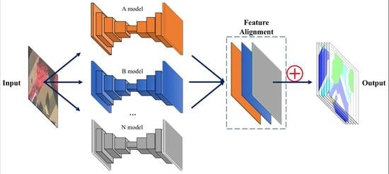
Stacked Fully Convolutional Networks
- Alignment loss ()Through the FCN-based model, extracted features (denoted as ) with size of are generated. W and H is consistent with the height and width of the input. The value of D is the same as the number of classes of land covers. The maximum and minimum value for each position from the 1st to the feature are computed. The final alignment loss () is calculated by the mean square error between corresponding maximum and minimum values of all positions.
- Segmentation loss ()From all extracted features (), the final output/prediction(Y) of the network is computed by taking the average value of all features. Then, the binary cross entropy [54], which calculates the difference between ground truth(G) and its corresponding prediction, is used as segmentation loss(). The calculation can be formulated aswhere and represent the (i,j,k) element of model output(Y) and ground truth (G). The value of is the predicted probability of the pixel category.
2.3. Experimental Set-Up
2.3.1. Network Specification
- FCN-8s. The classic FCN-8s architecture was proposed by Long et al. in 2015 [26]. This method innovatively adopts fully convolutional architecture to perform pixel-to-pixel image classification or segmentation. The FCN architecture is the first fully convolutional network used for image segmentation.
- U-Net. The U-Net architecture was proposed by Ronneberger et al. [30] for medical image segmentation. This method introduces multiple skip connections between upper and downer layers. Owing to its robustness and elegant structure, U-Net and its variants are widely adopted for many semantic segmentation tasks.
- FPN. The FPN architecture was published by Lin et al., 2017 [31]. Like U-Net, this method adopts multiple skip connections. In addition, the FPN model generates multi-scale predictions for final output. By utilizing abundant information from the feature pyramid, the FPN method achieves state-of-the-art performance.
2.3.2. Model Setup
3. Results
3.1. Sensitivity Analysis of Feature Alignment
3.2. Performances Comparison
3.3. Qualitative Comparison
3.4. Computational Efficiency
4. Discussions
4.1. Regarding the Proposed Feature Alignment Framework
4.2. Accuracies, Uncertainties, and Limitations
5. Conclusions
Author Contributions
Acknowledgments
Conflicts of Interest
Abbreviations
| CNN | Convolutional Neural Network |
| FCN | Fully Convolutional Networks |
| SFCN | Stacked Fully Convolutional Networks |
| FPN | Feature Pyramid Networks |
| FA | Feature Alignment |
References
- Yang, X.; Wu, Y.; Dang, H. Urban Land Use Efficiency and Coordination in China. Sustainability 2017, 9, 410. [Google Scholar] [CrossRef]
- Abbott, E.; Powell, D. Land-vehicle navigation using GPS. Proc. IEEE 1999, 87, 145–162. [Google Scholar] [CrossRef]
- Stow, D.A.; Hope, A.; McGuire, D.; Verbyla, D.; Gamon, J.; Huemmrich, F.; Houston, S.; Racine, C.; Sturm, M.; Tape, K.; et al. Remote sensing of vegetation and land-cover change in Arctic Tundra Ecosystems. Remote Sens. Environ. 2004, 89, 281–308. [Google Scholar] [CrossRef] [Green Version]
- Heilman, G.E.; Strittholt, J.R.; Slosser, N.C.; Dellasala, D.A. Forest Fragmentation of the Conterminous United States: Assessing Forest Intactness through Road Density and Spatial Characteristics: Forest fragmentation can be measured and monitored in a powerful new way by combining remote sensing, geographic information systems, and analytical software. AIBS Bull. 2002, 52, 411–422. [Google Scholar]
- Hamre, L.N.; Domaas, S.T.; Austad, I.; Rydgren, K. Land-cover and structural changes in a western Norwegian cultural landscape since 1865, based on an old cadastral map and a field survey. Landsc. Ecol. 2007, 22, 1563–1574. [Google Scholar] [CrossRef]
- Colomina, I.; Molina, P. Unmanned aerial systems for photogrammetry and remote sensing: A review. ISPRS J. Photogramm. Remote Sens. 2014, 92, 79–97. [Google Scholar] [CrossRef] [Green Version]
- Ma, L.; Li, M.; Ma, X.; Cheng, L.; Du, P.; Liu, Y. A review of supervised object-based land-cover image classification. ISPRS J. Photogramm. Remote Sens. 2017, 130, 277–293. [Google Scholar] [CrossRef]
- Glasbey, C.A. An analysis of histogram-based thresholding algorithms. CVGIP: Graph. Model. Image Process. 1993, 55, 532–537. [Google Scholar] [CrossRef]
- Kanopoulos, N.; Vasanthavada, N.; Baker, R.L. Design of an image edge detection filter using the Sobel operator. IEEE J. Solid-State Circuits 1988, 23, 358–367. [Google Scholar] [CrossRef]
- Canny, J. A computational approach to edge detection. In Readings in Computer Vision; Elsevier: New York, NY, USA, 1987; pp. 184–203. [Google Scholar]
- Wu, Z.; Leahy, R. An optimal graph theoretic approach to data clustering: Theory and its application to image segmentation. IEEE Trans. Pattern Anal. Mach. Intell. 1993, 15, 1101–1113. [Google Scholar] [CrossRef]
- Zhen, D.; Zhongshan, H.; Jingyu, Y.; Zhenming, T. FCM Algorithm for the Research of Intensity Image Segmentation. Acta Electron. Sin. 1997, 5, 39–43. [Google Scholar]
- Tremeau, A.; Borel, N. A region growing and merging algorithm to color segmentation. Pattern Recognit. 1997, 30, 1191–1203. [Google Scholar] [CrossRef]
- Ozer, S.; Langer, D.L.; Liu, X.; Haider, M.A.; van der Kwast, T.H.; Evans, A.J.; Yang, Y.; Wernick, M.N.; Yetik, I.S. Supervised and unsupervised methods for prostate cancer segmentation with multispectral MRI. Med. Phys. 2010, 37, 1873–1883. [Google Scholar] [CrossRef]
- Li, M.; Zang, S.; Zhang, B.; Li, S.; Wu, C. A review of remote sensing image classification techniques: The role of spatio-contextual information. Eur. J. Remote Sens. 2014, 47, 389–411. [Google Scholar] [CrossRef]
- Viola, P.; Jones, M. Rapid Object Detection Using a Boosted Cascade of Simple Features. In Proceedings of the 2001 IEEE Computer Society Conference on Computer Vision and Pattern Recognition (CVPR 2001), Kauai, HI, USA, 8–14 December 2001; IEEE: Piscataway, NJ, USA, 2001; Volume 1, p. I. [Google Scholar]
- Lowe, D.G. Object recognition from local scale-invariant features. In Proceedings of the Seventh IEEE International Conference on Computer Vision, Kerkyra, Greece, 20–27 September 1999; IEEE: Piscataway, NJ, USA, 1999; Volume 2, pp. 1150–1157. [Google Scholar]
- Ojala, T.; Pietikainen, M.; Maenpaa, T. Multiresolution gray-scale and rotation invariant texture classification with local binary patterns. IEEE Trans. Pattern Anal. Mach. Intell. 2002, 24, 971–987. [Google Scholar] [CrossRef] [Green Version]
- Dalal, N.; Triggs, B. Histograms of oriented gradients for human detection. In Proceedings of the 2005 IEEE Computer Society Conference on Computer Vision and Pattern Recognition (CVPR 2005), San Diego, CA, USA, 20–26 June 2005; IEEE: Piscataway, NJ, USA, 2005; Volume 1, pp. 886–893. [Google Scholar]
- Inglada, J. Automatic recognition of man-made objects in high resolution optical remote sensing images by SVM classification of geometric image features. ISPRS J. Photogramm. Remote Sens. 2007, 62, 236–248. [Google Scholar] [CrossRef]
- Aytekin, Ö.; Zöngür, U.; Halici, U. Texture-based airport runway detection. IEEE Geosci. Remote Sens. Lett. 2013, 10, 471–475. [Google Scholar] [CrossRef]
- Dong, Y.; Du, B.; Zhang, L. Target detection based on random forest metric learning. IEEE J. Sel. Top. Appl. Earth Obs. Remote Sens. 2015, 8, 1830–1838. [Google Scholar] [CrossRef]
- Gletsos, M.; Mougiakakou, S.G.; Matsopoulos, G.K.; Nikita, K.S.; Nikita, A.S.; Kelekis, D. A computer-aided diagnostic system to characterize CT focal liver lesions: Design and optimization of a neural network classifier. IEEE Trans. Inf. Technol. Biomed. 2003, 7, 153–162. [Google Scholar] [CrossRef] [PubMed]
- LeCun, Y.; Bengio, Y. Convolutional networks for images, speech, and time series. Handb. Brain Theory Neural Networks 1995, 3361, 1995. [Google Scholar]
- Ciresan, D.; Giusti, A.; Gambardella, L.M.; Schmidhuber, J. Deep neural networks segment neuronal membranes in electron microscopy images. In Advances in Neural Information Processing Systems; 2012; pp. 2843–2851. Available online: https://papers.nips.cc/paper/4741-deep-neural-networks-segment-neuronal-membranes-in-electron-microscopy-images (accessed on 1 March 2019).
- Long, J.; Shelhamer, E.; Darrell, T. Fully convolutional networks for semantic segmentation. In Proceedings of the IEEE Conference on Computer Vision and Pattern Recognition, Boston, MA, USA, 7–12 June 2015; IEEE: Piscataway, NJ, USA, 2015; pp. 3431–3440. [Google Scholar] [Green Version]
- Guo, Z.; Shao, X.; Xu, Y.; Miyazaki, H.; Ohira, W.; Shibasaki, R. Identification of village building via Google Earth images and supervised machine learning methods. Remote Sens. 2016, 8, 271. [Google Scholar] [CrossRef]
- Kampffmeyer, M.; Salberg, A.B.; Jenssen, R. Semantic segmentation of small objects and modeling of uncertainty in urban remote sensing images using deep convolutional neural networks. In Proceedings of the IEEE Conference on Computer Vision and Pattern Recognition Workshops, Las Vegas, NV, USA, 26 June–1 July 2016; IEEE: Piscataway, NJ, USA, 2016; pp. 1–9. [Google Scholar]
- Li, L.; Liang, J.; Weng, M.; Zhu, H. A Multiple-Feature Reuse Network to Extract Buildings from Remote Sensing Imagery. Remote Sens. 2018, 10, 1350. [Google Scholar] [CrossRef]
- Ronneberger, O.; Fischer, P.; Brox, T. U–Net: Convolutional networks for biomedical image segmentation. In International Conference on Medical Image Computing and Computer-Assisted Intervention; Springer: Cham, Switherland, 2015; pp. 234–241. [Google Scholar]
- Lin, T.Y.; Dollár, P.; Girshick, R.; He, K.; Hariharan, B.; Belongie, S. Feature pyramid networks for object detection. In Proceedings of the IEEE Conference on Computer Vision and Pattern Recognition, Honolulu, HI, USA, 22–15 July 2017; IEEE: Piscataway, NJ, USA, 2017; Volume 1, p. 4. [Google Scholar]
- Noh, H.; Hong, S.; Han, B. Learning deconvolution network for semantic segmentation. In Proceedings of the IEEE International Conference on Computer Vision, Santiago, Chile, 13–16 December 2015; IEEE: Piscataway, NJ, USA, 2017; pp. 1520–1528. [Google Scholar]
- Wu, G.; Shao, X.; Guo, Z.; Chen, Q.; Yuan, W.; Shi, X.; Xu, Y.; Shibasaki, R. Automatic Building Segmentation of Aerial Imagery Using Multi-Constraint Fully Convolutional Networks. Remote Sens. 2018, 10, 407. [Google Scholar] [CrossRef]
- Wu, G.; Guo, Z.; Shi, X.; Chen, Q.; Xu, Y.; Shibasaki, R.; Shao, X. A Boundary Regulated Network for Accurate Roof Segmentation and Outline Extraction. Remote Sens. 2018, 10, 1195. [Google Scholar] [CrossRef]
- Tetko, I.V.; Livingstone, D.J.; Luik, A.I. Neural network studies. 1. Comparison of overfitting and overtraining. J. Chem. Inf. Comput. Sci. 1995, 35, 826–833. [Google Scholar] [CrossRef]
- Prechelt, L. Automatic early stopping using cross validation: Quantifying the criteria. Neural Networks 1998, 11, 761–767. [Google Scholar] [CrossRef]
- Prechelt, L. Early stopping-but when? In Neural Networks: Tricks of the Trade; Springer: Cham, Switherland, 1998; pp. 55–69. [Google Scholar]
- Wong, S.C.; Gatt, A.; Stamatescu, V.; McDonnell, M.D. Understanding Data Augmentation for Classification: When to Warp? In Proceedings of the International Conference on Digital Image Computing: Techniques and Applications (DICTA), Surfers Paradise, QLD, Australia, 30 November–2 December 2016; IEEE: Piscataway, NJ, USA, 2016; pp. 1–6. [Google Scholar] [Green Version]
- Grasmair, M.; Scherzer, O.; Haltmeier, M. Necessary and sufficient conditions for linear convergence of l1-regularization. Commun. Pure Appl. Math. 2011, 64, 161–182. [Google Scholar] [CrossRef]
- Ng, A.Y. Feature selection, L 1 vs. L 2 regularization, and rotational invariance. In Proceedings of the 21st International Conference on Machine Learning, Banff, AB, Canada, 4–8 July 2004; ACM: New York, NY, USA, 2004; p. 78. [Google Scholar]
- Srivastava, N.; Hinton, G.; Krizhevsky, A.; Sutskever, I.; Salakhutdinov, R. Dropout: A simple way to prevent neural networks from overfitting. J. Mach. Learn. Res. 2014, 15, 1929–1958. [Google Scholar]
- Rosen, B.E. Ensemble learning using decorrelated neural networks. Connect. Sci. 1996, 8, 373–384. [Google Scholar] [CrossRef]
- Guo, Z.; Chen, Q.; Wu, G.; Xu, Y.; Shibasaki, R.; Shao, X. Village Building Identification Based on Ensemble Convolutional Neural Networks. Sensors 2017, 17, 2487. [Google Scholar] [CrossRef] [PubMed]
- Polak, M.; Zhang, H.; Pi, M. An evaluation metric for image segmentation of multiple objects. Image Vis. Comput. 2009, 27, 1223–1227. [Google Scholar] [CrossRef]
- Carletta, J. Assessing agreement on classification tasks: The kappa statistic. Comput. Linguist. 1996, 22, 249–254. [Google Scholar]
- Li, E.; Femiani, J.; Xu, S.; Zhang, X.; Wonka, P. Robust rooftop extraction from visible band images using higher order CRF. IEEE Trans. Geosci. Remote Sens. 2015, 53, 4483–4495. [Google Scholar] [CrossRef]
- Comer, M.L.; Delp, E.J. Morphological operations for color image processing. J. Electron. Imaging 1999, 8, 279–290. [Google Scholar] [CrossRef]
- Lin, T.Y.; Maire, M.; Belongie, S.; Hays, J.; Perona, P.; Ramanan, D.; Dollár, P.; Zitnick, C.L. Microsoft coco: Common objects in context. In Proceedings of the 13th European Conference on Computer Vision(ECCV 2014), Zurich, Switzerland, 6–12 September 2014; Springer: Cham, Switherland, 2014; pp. 740–755. [Google Scholar]
- Everingham, M.; Van Gool, L.; Williams, C.K.; Winn, J.; Zisserman, A. The pascal visual object classes (voc) challenge. Int. J. Comput. Vis. 2010, 88, 303–338. [Google Scholar] [CrossRef]
- Nair, V.; Hinton, G.E. Rectified linear units improve restricted boltzmann machines. In Proceedings of the 27th International Conference on Machine Learning (ICML-10), Haifa, Israel, 21–24 June 2010; Omnipress: Madison, WI, USA, 2010; pp. 807–814. [Google Scholar]
- Ioffe, S.; Szegedy, C. Batch normalization: Accelerating deep network training by reducing internal covariate shift. In Proceedings of the International Conference on Machine Learning, Lille, France, 6–11 July 2015; pp. 448–456. [Google Scholar]
- Nagi, J.; Ducatelle, F.; Di Caro, G.A.; Cireşan, D.; Meier, U.; Giusti, A.; Nagi, F.; Schmidhuber, J.; Gambardella, L.M. Max-pooling convolutional neural networks for vision-based hand gesture recognition. In Proceedings of the 2011 IEEE International Conference on Signal and Image Processing Applications (ICSIPA 2011), Kuala Lumpur, Malaysia, 16–18 November 2011; IEEE: Piscataway, NJ, USA, 2011; pp. 342–347. [Google Scholar] [Green Version]
- Novak, K. Rectification of digital imagery. Photogramm. Eng. Remote Sens. 1992, 58, 339. [Google Scholar]
- Shore, J.; Johnson, R. Properties of cross-entropy minimization. IEEE Trans. Inf. Theory 1981, 27, 472–482. [Google Scholar] [CrossRef] [Green Version]
- Kingma, D.P.; Ba, J. Adam: A method for stochastic optimization. arXiv 2014, arXiv:1412.6980. [Google Scholar]
- Wu, G.; Guo, Z. Geoseg: A Computer Vision Package for Automatic Building Segmentation and Outline Extraction. arXiv 2018, arXiv:1809.03175. [Google Scholar]
- Maggiori, E.; Tarabalka, Y.; Charpiat, G.; Alliez, P. Convolutional neural networks for large-scale remote-sensing image classification. IEEE Trans. Geosci. Remote Sens. 2017, 55, 645–657. [Google Scholar] [CrossRef]
- Maggiori, E.; Tarabalka, Y.; Charpiat, G.; Alliez, P. Fully convolutional networkss for remote sensing image classification. In Proceedings of the 2016 IEEE International Geoscience and Remote Sensing Symposium (IGARSS), Beijing, China, 10–15 July 2016; pp. 5071–5074. [Google Scholar]
- Demir, I.; Koperski, K.; Lindenbaum, D.; Pang, G.; Huang, J.; Basu, S.; Hughes, F.; Tuia, D.; Raskar, R. Deepglobe 2018: A challenge to parse the earth through satellite images. arXiv 2018, arXiv:1805.06561. [Google Scholar]
- Chen, Q.; Wang, L.; Wu, Y.; Wu, G.; Guo, Z.; Waslander, S.L. Aerial imagery for roof segmentation: A large-scale dataset towards automatic mapping of buildings. ISPRS J. Photogramm. Remote Sens. 2019, 147, 42–55. [Google Scholar] [CrossRef]


| Land-covers | RGB Values |
|---|---|
| Impervious surfaces | [255, 255, 255] |
| Building | [0, 0, 255] |
| Low vegetation | [0, 255, 255] |
| Tree | [0, 255, 0] |
| Car | [255, 255, 0] |
| Clutter/Background | [255, 0, 0] |
| Version | No. of basic models | FCN-8s | U-Net | FPN |
|---|---|---|---|---|
| SFCNf&p | 2 | + | − | + |
| SFCNf&u | 2 | + | + | − |
| SFCNu&p | 2 | + | + | − |
| SFCNf&u&p | 3 | + | + | + |
| Method | F1-Score | Jaccard Index | Kappa Coefficient | ||||
|---|---|---|---|---|---|---|---|
| Version | λ-Value | Mean | SD | Mean | SD | Mean | SD |
| SFCNf&p | 0.0 | 0.738 | 0.003 | 0.584 | 0.004 | 0.685 | 0.004 |
| 0.2 | 0.748 | 0.002 | 0.598 | 0.003 | 0.698 | 0.003 | |
| 0.4 | 0.761 | 0.004 | 0.615 | 0.004 | 0.714 | 0.004 | |
| 0.6 | 0.764 | 0.004 | 0.619 | 0.004 | 0.717 | 0.004 | |
| 0.8 | 0.767 | 0.002 | 0.623 | 0.002 | 0.721 | 0.002 | |
| 1.0 | 0.767 | 0.003 | 0.623 | 0.003 | 0.721 | 0.003 | |
| SFCNf&u | 0.0 | 0.741 | 0.003 | 0.589 | 0.004 | 0.689 | 0.004 |
| 0.2 | 0.764 | 0.002 | 0.619 | 0.002 | 0.717 | 0.002 | |
| 0.4 | 0.762 | 0.003 | 0.616 | 0.004 | 0.715 | 0.004 | |
| 0.6 | 0.762 | 0.004 | 0.615 | 0.005 | 0.714 | 0.004 | |
| 0.8 | 0.772 | 0.003 | 0.629 | 0.004 | 0.727 | 0.004 | |
| 1.0 | 0.770 | 0.001 | 0.626 | 0.002 | 0.723 | 0.002 | |
| SFCNu&p | 0.0 | 0.765 | 0.006 | 0.619 | 0.007 | 0.718 | 0.006 |
| 0.2 | 0.772 | 0.004 | 0.629 | 0.006 | 0.727 | 0.005 | |
| 0.4 | 0.772 | 0.006 | 0.629 | 0.008 | 0.726 | 0.007 | |
| 0.6 | 0.780 | 0.001 | 0.639 | 0.002 | 0.736 | 0.001 | |
| 0.8 | 0.785 | 0.004 | 0.646 | 0.005 | 0.742 | 0.005 | |
| 1.0 | 0.784 | 0.001 | 0.645 | 0.002 | 0.741 | 0.002 | |
| SFCNf&u&p | 0.0 | 0.773 | 0.006 | 0.630 | 0.007 | 0.727 | 0.006 |
| 0.2 | 0.780 | 0.002 | 0.638 | 0.002 | 0.735 | 0.002 | |
| 0.4 | 0.780 | 0.001 | 0.640 | 0.001 | 0.736 | 0.001 | |
| 0.6 | 0.778 | 0.002 | 0.637 | 0.002 | 0.734 | 0.002 | |
| 0.8 | 0.778 | 0.001 | 0.637 | 0.002 | 0.733 | 0.001 | |
| 1.0 | 0.780 | 0.001 | 0.640 | 0.002 | 0.736 | 0.002 | |
| Group | F1-Score | Jaccard Index | Kappa Coefficient | |||
|---|---|---|---|---|---|---|
| t-Value | p-Value | t-Value | p-Value | t-Value | p-Value | |
| SFCNf&p (+FA vs.−FA ) | 14.438 | 0.0001 | 16.546 | 0.0001 | 15.123 | 0.0001 |
| SFCNf&u (+FA vs.−FA ) | 11.750 | 0.0003 | 11.558 | 0.0003 | 11.144 | 0.0004 |
| SFCNu&p (+FA vs.−FA ) | 5.350 | 0.0059 | 5.329 | 0.0060 | 5.210 | 0.0065 |
| SFCNf&u&p (+FA vs.−FA ) | 2.234 | 0.0892 | 2.271 | 0.0856 | 2.415 | 0.0732 |
| Methods | Training FPS | Testing FPS | ||
|---|---|---|---|---|
| Mean | SD | Mean | SD | |
| FCN-8s | 41.4 | 0.2 | 67.1 | 0.3 |
| U-Net | 59.4 | 0.4 | 75.4 | 1.3 |
| FPN | 54.6 | 2.0 | 74.7 | 4.4 |
| SFCNf&p | 31.2 | 0.2 | 61.7 | 0.7 |
| SFCNf&u | 33.4 | 0.8 | 63.2 | 0.9 |
| SFCNu&p | 41.8 | 0.9 | 67.7 | 3.0 |
| SFCNf&u&p | 27.2 | 0.2 | 57.6 | 0.1 |
© 2019 by the authors. Licensee MDPI, Basel, Switzerland. This article is an open access article distributed under the terms and conditions of the Creative Commons Attribution (CC BY) license (http://creativecommons.org/licenses/by/4.0/).
Share and Cite
Wu, G.; Guo, Y.; Song, X.; Guo, Z.; Zhang, H.; Shi, X.; Shibasaki, R.; Shao, X. A Stacked Fully Convolutional Networks with Feature Alignment Framework for Multi-Label Land-cover Segmentation. Remote Sens. 2019, 11, 1051. https://doi.org/10.3390/rs11091051
Wu G, Guo Y, Song X, Guo Z, Zhang H, Shi X, Shibasaki R, Shao X. A Stacked Fully Convolutional Networks with Feature Alignment Framework for Multi-Label Land-cover Segmentation. Remote Sensing. 2019; 11(9):1051. https://doi.org/10.3390/rs11091051
Chicago/Turabian StyleWu, Guangming, Yimin Guo, Xiaoya Song, Zhiling Guo, Haoran Zhang, Xiaodan Shi, Ryosuke Shibasaki, and Xiaowei Shao. 2019. "A Stacked Fully Convolutional Networks with Feature Alignment Framework for Multi-Label Land-cover Segmentation" Remote Sensing 11, no. 9: 1051. https://doi.org/10.3390/rs11091051