Improved Automated Detection of Subpixel-Scale Inundation—Revised Dynamic Surface Water Extent (DSWE) Partial Surface Water Tests


U.S. Geological Survey, 415 National Center, Reston, VA 20192, USA
Remote Sens. 2019, 11(4), 374; https://doi.org/10.3390/rs11040374
Submission received: 11 October 2018
/
Revised: 4 December 2018
/
Accepted: 6 December 2018
/
Published: 13 February 2019
(This article belongs to the Section Remote Sensing in Geology, Geomorphology and Hydrology)
Abstract
:In order to produce useful hydrologic and aquatic habitat data from the Landsat system, the U.S. Geological Survey has developed the “Dynamic Surface Water Extent” (DSWE) Landsat Science Product. DSWE will provide long-term, high-temporal resolution data on variations in inundation extent. The model used to generate DSWE is composed of five decision-rule based tests that do not require scene-based training. To allow its general application, required inputs are limited to the Landsat at-surface reflectance product and a digital elevation model. Unlike other Landsat-based water products, DSWE includes pixels that are only partially covered by water to increase inundation dynamics information content. Previously published DSWE model development included one wetland-focused test developed through visual inspection of field-collected Everglades spectra. A comparison of that test’s output against Everglades Depth Estimation Network (EDEN) in situ data confirmed the expectation that omission errors were a prime source of inaccuracy in vegetated environments. Further evaluation exposed a tendency toward commission error in coniferous forests. Improvements to the subpixel level “partial surface water” (PSW) component of DSWE was the focus of this research. Spectral mixture models were created from a variety of laboratory and image-derived endmembers. Based on the mixture modeling, a more “aggressive” PSW rule improved accuracy in herbaceous wetlands and reduced errors of commission elsewhere, while a second “conservative” test provides an alternative when commission errors must be minimized. Replication of the EDEN-based experiments using the revised PSW tests yielded a statistically significant increase in mean overall agreement (4%, p = 0.01, n = 50) and a statistically significant decrease (11%, p = 0.009, n = 50) in mean errors of omission. Because the developed spectral mixture models included image-derived vegetation endmembers and laboratory spectra for soil groups found across the US, simulations suggest where the revised DSWE PSW tests perform as they do in the Everglades and where they may prove problematic. Visual comparison of DSWE outputs with an unusual variety of coincidently collected images for locations spread throughout the US support conclusions drawn from Everglades quantitative analyses and highlight DSWE PSW component strengths and weaknesses.

1. Introduction
With the release of the Landsat Archive and on-going Landsat/Sentinel data collects at no cost to the user [1], great progress is being made in the development of long-term databases on inundation, including data summarizing the probability of surface water occurrence at continental [2] and global [3] scales. However, these products primarily represent the occurrence of open surface water at Landsat pixel resolution and do not specifically target the detection of inundation when vegetation is present at the subpixel scale [4,5]. Therefore, they may not adequately characterize vegetated wetland inundation dynamics that are important in energy and biogeochemical fluxes, habitat characterization, and natural disaster response [4,5]. The U.S. Geological Survey (USGS) is producing value-added products from Landsat data to facilitate science and resource management. One product named Dynamic Surface Water Extent (DSWE) is designed to provide high temporal, moderate spatial resolution long-term data on terrestrial surface inundation. For DSWE product generation, each cloud-, cloud shadow-, and snow-free pixel in a given scene is tested for the presence of standing surface water and classified into either “not water” (NW) or separate “open water” (OW) and “partial surface water” (OSW) classes. Through the application of DSWE, potentially every cloud-, shadow-, and snow-free pixel in the Landsat Archive could be tested for the presence or absence of surface water at subpixel scale. The resulting historic and on-going data records will be useful for a wide variety of hydrology, climate, and ecology scientific research, as well as for water and land resource management purposes.
A discussion of the philosophy underpinning DSWE model development, the theoretical basis for its “open water” (pure water pixel) tests, and DSWE product characteristics, are briefly described here. DSWE was designed to require no scene-based training data [4] and with such basic inputs as to potentially be applied globally should its accuracy prove suitable. The quality data included with the input Landsat reflectance product, namely flags for cloud, cloud shadow, and snow, are used to apply masking that mitigates the adverse effects of these features on DSWE model output (as discussed further in Section 3.3). Similarly, the digital elevation model (DEM) is used to mask terrain-induced shadow. The entire DSWE model that is currently (2018) being used for data production consists of five tests: three are designed to detect whether each Landsat pixel is entirely covered by water. These are termed Open Water (OW) tests. Two additional ones, termed Partial Surface Water (PSW) tests, which are the focus of this manuscript, are designed to detect inundation in the presence of vegetation or other non-water land covers at Landsat subpixel scale. For clarity, output from the first generation of the DSWE model is referred to as “prototype DSWE” and the prototype PSW test is referred to as “PSW v1”, while the revised tests detailed here are collectively referred to as the “PSW v2”.
In addition to the prior quantitative assessment of the PSW v1 [4], prototype DSWE data have been employed in a wide variety of scientific and resource management applications. Examples to-date include characterizing tundra surface water dynamics [6], estimating river discharge by satellite [7], and providing automated training for other surface water mapping algorithms that use optical [5] and RADAR [8] satellite data. However, as was originally hypothesized, DSWE PSW v1 uncertainty is biased toward omission error [4]. Visual examination of the prototype data generated across a broad set of sites in the US (Figure 1) further indicated that the PSW v1 test was prone to commission error in forested environments (as illustrated in Section 3.3). Although these errors did not adversely impact the applications to which the prototype data were applied, the wetland inundation component of DSWE is here reexamined to address these errors and revised to improve overall DSWE model performance.
Goal and Objectives
The goal of the research detailed here was to improve the PSW detection component of the DSWE model. This improvement was pursued in five steps. First, more robust testing of the DSWE PSW component was enabled through the construction of spectral mixture models based on sample image-derived vegetation spectral endmembers and a broad range of soils represented by laboratory spectra. Second, based on that mixture modeling, two new PSW tests were formulated—one “conservative” (PSW v2-Cons)—to reduce commission errors in coniferous forested environments and the other “aggressive” (PSW v2-Aggrsv) to reduce omission errors in marshland environments. Third, ternary graphs were used to visualize the performance of the PSW v2 tests for a variety of vegetation and soil mixtures and as a function of Landsat imaging sensor type. Fourth, primary components of the experiment documented in Jones [4] were replicated to compare PSW v2 results to PSW v1 results. And fifth, output from the revised DSWE model were generated for every chip shown in Figure 1 and compared against prototype output as well as other geospatial data, particularly contemporaneous satellite and airborne imagery, to qualitatively assess its robustness across a range of environments and sun angle conditions.
The methods section describes the spectral library and spectral mixing model created for DSWE PSW v2 test development. It also illustrates how the model results were visualized using ternary graphing techniques to explore test performance given various combinations of land cover and soils. The methods section also briefly recounts the approach to wetland-focused evaluation that was detailed previously [4] and introduces the visual cross-image comparison process. The results and interpretation of the simulations and empirical experiments are provided in the results and discussion section before caveats on DSWE PSW v2 use are provided in the conclusions and recommendations section.
2. Methods
2.1. Spectral Mixture Modeling
The application of long time-series data from Landsat and other openly available satellite data has rapidly increased in recent years [9]. Reviews of satellite remote sensing of inland surface waters and wetlands identify the multitude of techniques used [9,10]. When subpixel-scale mixtures are of interest, most rely on the application of machine learning algorithms against large amounts of training data selected either from the imagery to be classified or from independent sources that are often higher spatial resolution image data [11,12,13]. However, spectral mixture modeling [14] has been applied to Landsat for subpixel wetland vegetation/condition assessment [15,16,17,18,19] and inland inundation monitoring [20,21,22,23,24,25,26]. Because it is a physically based approach [27], spectral mixture modeling may be used to establish theoretical reflectance data from which DSWE model decision rules could be drawn–thereby eliminating the need for extensive (and therefore costly) training data collection. Linear spectral mixture modeling, which assumes the reflectance of any pixel is a result of a spatially weighted sum of its constituent fractions, is attractive as a subpixel cover estimation technique given its relative mathematical simplicity and yet, sufficient accuracy compared to more complex approaches [28,29]. The sampling of a wide variety of Enhanced Thematic Mapper (ETM) spectra from diverse Landsat scenes spaced across the Earth has shown that linear spectral modeling could represent a majority of their variation given 3 endmembers: soil/rock substrate, vegetation, and ‘dark surface reflectance spectra’ [30]. The latter endmember would include shadows, soils and certain water surfaces.
For DSWE PSW v2 model development, the linear spectral mixture model represented by Equation (1) as taken from [31] was implemented in Microsoft Excel 2016 to facilitate intuitive visualization and threshold selection.
where is the reflectance of mixed water, soil, and vegetation in band ; , , and , respectively, are the reflectances of pure water, soil, and vegetation in band ; , , and , are the fractions (in percent) of water, soil, and vegetation, respectively [31].
Templates were created that calculated reflectance as spatially weighted combinations of the water, soil and vegetation in fractional cover increments of 10% for each constituent. And individual worksheets were created for each sensor (i.e., ETM or Operational Land Imager (OLI)), vegetation (herbaceous, coniferous forest, and mixed forest), and soil group combination (n = 96).
2.1.1. Input Spectral Data Development
The reflectance of wetland vegetation substrates can vary significantly and dynamically depending on water level and/or constituents, vegetation amount and type, and soil characteristics [20,32]. The spectra collected in situ in the Everglades, Florida, and used to develop the decision rule that was the PSW v1 test [4] were modified for PSW v2 test development. The response functions associated with Landsat Thematic Mapper (TM) and ETM sensors on-board Landsat 4 through 7 were compared and deemed sufficiently similar that ETM image-based spectra could be used to represent all Landsat TM/ETM class instruments. In contrast, the band passes and spectral response characteristics for Landsat 8 OLI are sufficiently different from those of the TM/ETM that OLI spectra were also derived for each cover type and soil group to allow evaluation of variation as a function of sensor. All treatments were replicated for ETM and OLI class sensors so variations in calculated reflectance and spectral indices that might result [33] could be accounted for and evaluated in the spectral mixture modeling.
2.1.2. Water Endmember
For the water spectral endmember, the purest sample possible as observed in the controlled environment of a laboratory was selected. The Advanced Spaceborne Thermal Emission and Reflection Radiometer (ASTER) library [34] as distributed with ENVI software (version 5.5) provided the water spectrum (named “tap-none-liquid-tap-water”) that was resampled to ETM and OLI spectral resolutions for DSWE PSW v2 development.
2.1.3. Soil Spectra
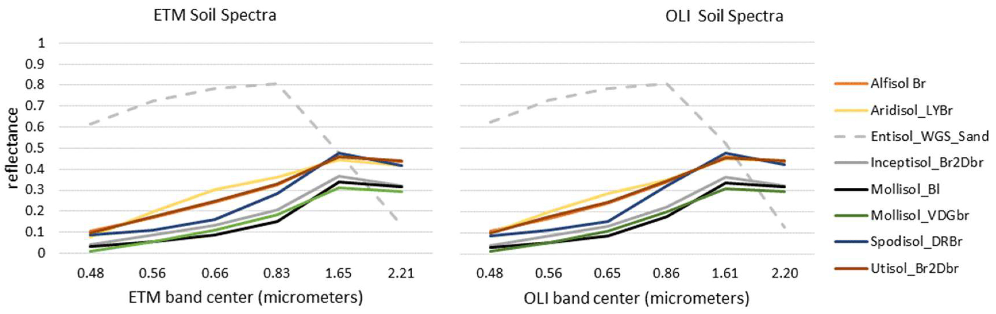
While the Everglades soil substrate ranges from very bright limestone to very dark peat soils [32], the potential variety of soil substrates found around the world were not well represented by the Everglades spectra, which were used for PSW v1 development. The potential impact of this variability was specifically addressed through the inclusion of a variety of soil spectra in PSW v2 development. Individual soil spectra found in the ASTER library [34] were grouped by dominant color/type (Table 1), averaged within type by wavelength at their original spectral resolution and then resampled within type to ETM and OLI bandwidths using ENVI. The resulting 16 spectra (8 soil groups and 2 sensors) are shown in Figure 2.
2.1.4. Vegetation Endmembers
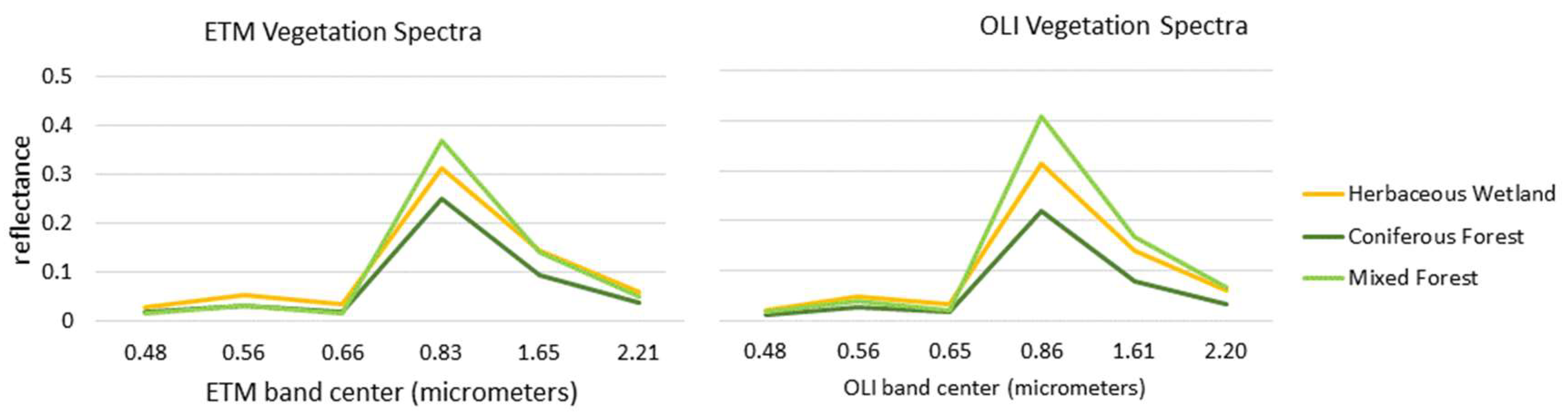
Collection of reflectance data from leaf samples in the laboratory fails to replicate the influence that structure (leaf orientation, layering) and associated shadowing have on vegetation spectra. Yet those canopy characteristics (and shadow in particular) have important effects on pixel reflectance measured at moderate spatial resolution, like that of Landsat satellite imagery [30,33,35]. Because field-collected vegetation spectra used for PSW v1 included shadow to a very limited extent, they were replaced with vegetation spectral endmembers carefully gathered from sample Landsat ETM and OLI scenes for PSW v2 development. The process used is portrayed in Figure 3. While Everglades-based spectra were still assumed to represent vegetation in herbaceous wetland environments, forested wetlands were represented by collecting image-based spectra from locations well outside the Everglades. Further, to minimize differences between ETM and OLI spectra that might be due to changes in vegetation, soil, or inundation conditions over time or space, areas of overlap between Landsat paths were exploited. That is, while there is potentially an 8-day difference between Landsat 7 and Landsat 8 overpasses for a single path/row, overpasses by the 2 satellites can occur on successive days (i.e., 1 day apart) for locations within the overlap between two different Landsat paths. Also, because vegetation endmembers were the targets [14,27], scenes captured when vegetation canopies exhibit greatest leaf biomass and vigor were optimal. Therefore, scenes lacking cloud cover, captured during the height of the growing season and, in the case of the Everglades, during a period of stable water levels were used. The vegetation endmembers of herbaceous wetland, mixed forest and coniferous forest were then collected from 3 sets of image pairs from across the US. The specific scenes used are listed in Table 2.
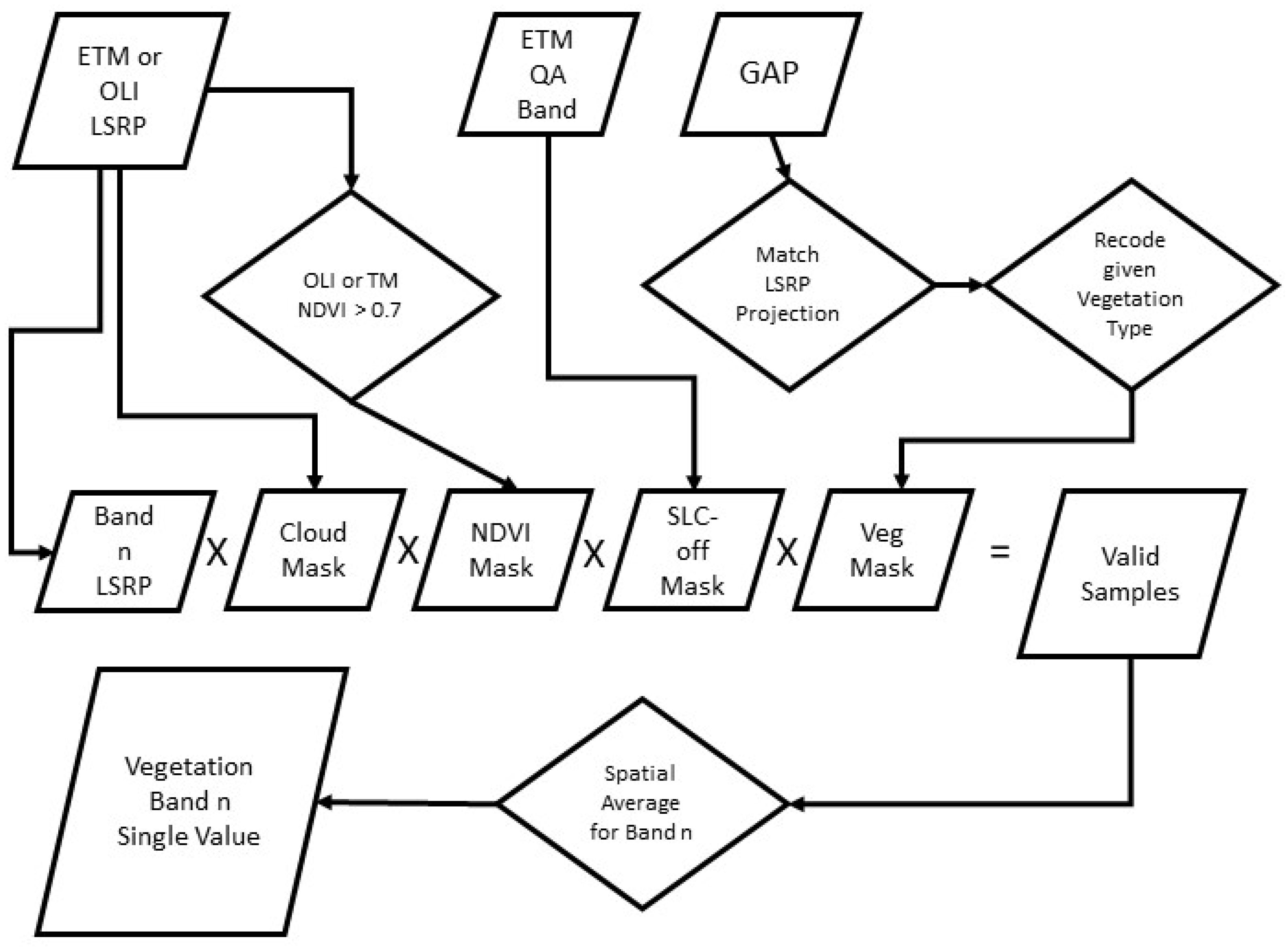
The inputs for vegetation endmember pixel selection were: calibrated and atmospherically corrected Landsat Surface Reflectance Product (LSRP) data with associated pixel quality indices [36,37]; USGS Gap Analysis Program (GAP) land cover data [38,39]; and normalized difference vegetation index (NDVI) [40] data calculated from the LSRP images. To minimize resampling of spectral data, the GAP data were re-projected to match each Albers-projected Landsat scene. Then a binary mask was created by reclassifying the target GAP class (Table 2) to 1 and all other GAP pixels to 0. Another binary mask was created to eliminate pixels of missing data in the Landsat 7 scene given the scanline corrector off (SLC-off) issue associated with Landsat 7 [41]. In turn, this mask was “snapped” to the OLI data to most accurately remove the same observations from the OLI input. A third mask was created based on the NDVI for both images in the pair. Pixels with a NDVI value equal to or greater than 0.7 were classified to 1 while all other pixels became 0. Once created, all masks were multiplied against one another at the pixel level to yield a final mask in which only pixels that met all quality, land cover, and vegetation index criteria across both images in the pair remained with a value of 1. As the final step, the averages of band reflectance values (i.e., on a band-by-band basis) for all remaining pixels were calculated. The resulting spectra are shown in Figure 4.
The ETM and OLI spectra for the water and all soils were exported as ASCII data from ENVI. The band-specific averages for the vegetation spectra were exported from Esri’s ArcMap (version 10.5) as ASCII. And all ASCII files were subsequently imported into Excel for further processing and analysis.
2.1.5. Snow/Ice Spectral Endmember
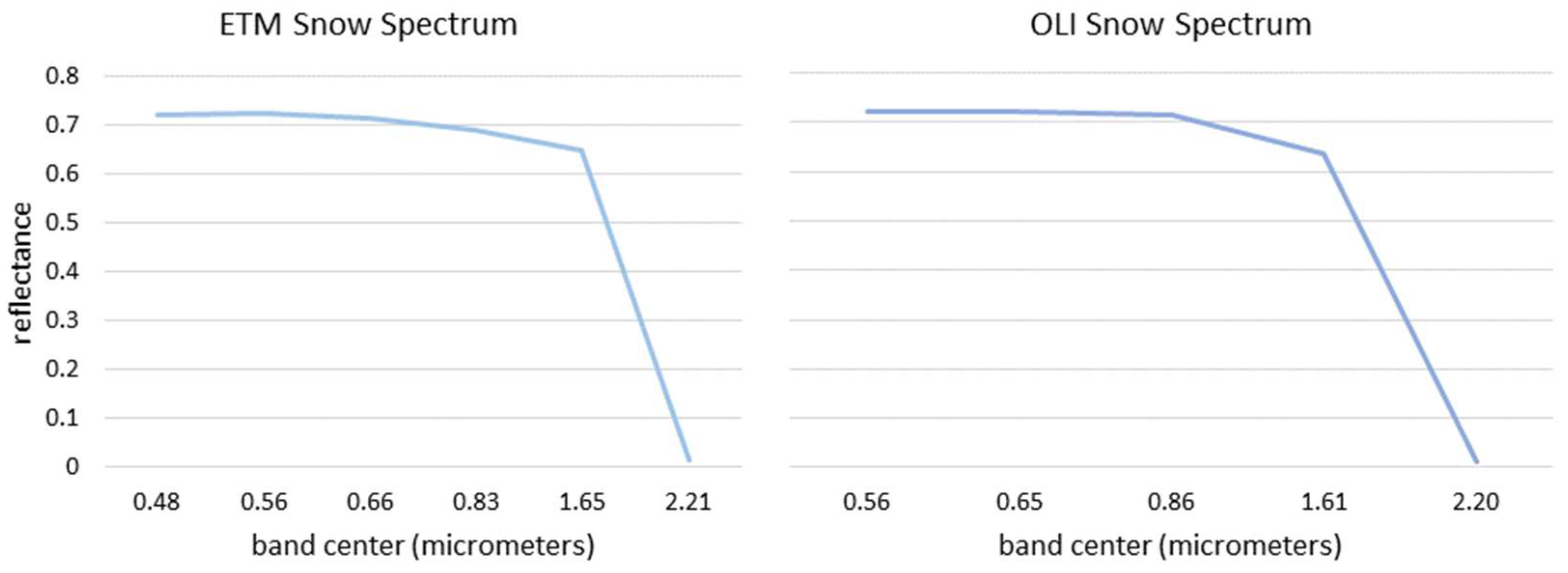
To evaluate the impact of snow and ice on DSWE PSW v2 tests, the process used to create spectral endmembers for water and soils was repeated using spectra from snow [42]. As noted in the metadata provided with the spectra, USGS researchers stored a 30-cm deep sample of very pure white snow (i.e., less than 1ppm particulate contamination) in a cooler before capturing spectra under controlled lighting in a laboratory while the snow melted over the course of several hours. The 16th spectra collected over the sample had as much as 3cm of water on its surface. Because an endmember of snow was desired for this modeling research, only the 5 spectra collected when the snow was dominantly snow (Table 3) were resampled to TM and OLI spectral band passes before being averaged on a by-band basis to yield a single spectral endmember per sensor as depicted in Figure 5.
2.2. DSWE partial surface water test development
A relatively simplistic approach that requires no scene-based training data is desirable so that detection of inundation through large amounts of satellite data is “automatic” and efficient [4]. Toward that end, indices useful for water and vegetation identification, such as the modified normalized difference wetness index or MNDWI [43] and NDVI were used in combination with thresholds on various bands to separate inundated from non-inundated pixels in the prototype DSWE model (v1) [4]. This approach was continued for the revision of the DSWE PSW decision rules. Spreadsheets for vegetation/soil combinations representative of herbaceous wetlands as well as mixed forest and coniferous swamplands were visually examined to establish thresholds and decision rules on various bands and indices that would detect increasingly smaller amounts of inundation within vegetation pixels without producing commission errors for mixtures dominated by soils. These rules were implemented through Excel equations with fields added to the worksheets to indicate thresholds, as well as which mixtures would result in water detections or non-detections given the decision rules employed. These thresholds were entered and/or modified in a ‘master’ worksheet for automatic propagation through all worksheets representing the various vegetation/soil/sensor combinations (n = 96).
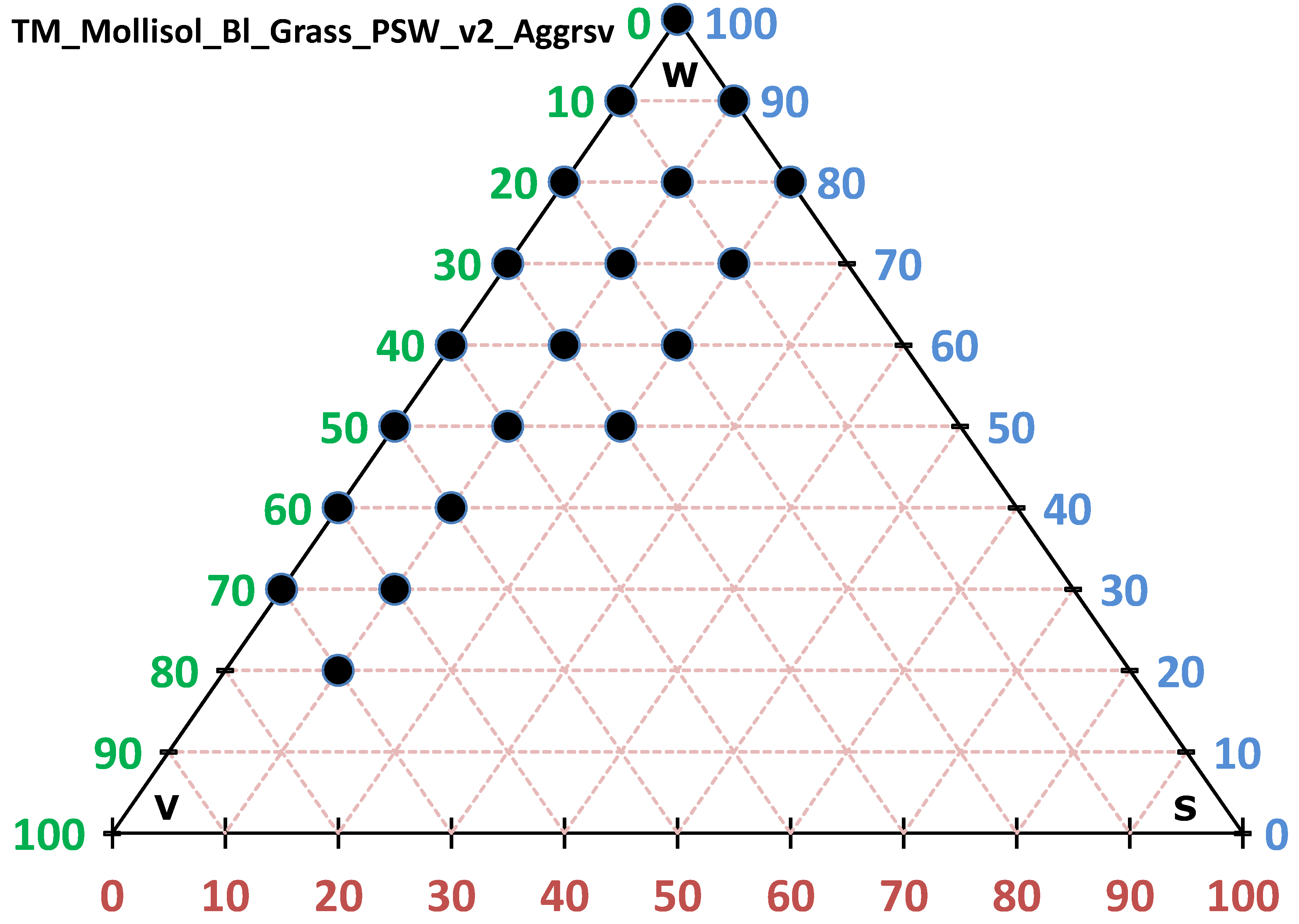
Next, to help visualize and understand the results and characteristics of these decision rule sets, ternary diagrams like that shown in Figure 6 were created for every sensor, soil, vegetation, and test combination. A mollisol soil example is provided in Figure 6 because that group covers the most area of any soil in the conterminous US [44]. For orientation, in Figure 6, the top point of the triangle represents a ‘mixture’ of 100% water, 0% vegetation, and 0% soil, while the lower left vertex is 100% vegetation, 0% water, and 0% soil. Concentrations for each constituent are interpreted by reading perpendicular to the constituent axis. The lowest black point in the diagram intersects the parallel directly below the top (water) vertex that represents a mixture of 20% water. To the right of the V labelled vertex, the point lies on the line that represents 70% vegetation. To the left of the S vertex, the point lies on the parallel line that represents 10% soil. As another example from Figure 6, when applied to simulated TM spectra of water, herbaceous vegetation, and mollisol black soil, PSW v2-Aggrsv declares “inundation” when the mixture is 20% water, 70% vegetation, and 10% soil.
2.3. DSWE PSW v2 Evaluation
To specifically measure whether the revised DSWE PSW tests represented an improvement over their predecessor, a subset of the Everglades Depth Estimation Network (EDEN) based experiments presented in [4] was replicated here. In addition, thousands of DSWE outputs were generated for areas across the county as shown in Figure 1, reviewed, and visually compared against a variety of other geospatial data products on wetlands, land cover, and in the form of remote sensed images from a variety of systems that could be readily interpreted. This section summarizes results of the Everglades quantitative analyses and illustrates results of the visual comparisons.
2.3.1. DSWE PSW v2 Point-based, Quantitative Assessment
Because it provides a uniquely extensive and rigorously collected record on inundated, vegetated landcover conditions, the previously documented [4] Florida Everglades point-based analysis was replicated using the DSWE v2 tests. For brevity, the method is only briefly recounted here. A set of 50 provisional level 1T Landsat 5 Surface Reflectance Product files (L5LSRP) that exhibit a broad range of cloud and inundation conditions were used to simulate real-world conditions for DSWE application. Table 4 shows the dates of satellite imagery.
A critical input to the method is water level (stage) for individual gages as provided by the EDEN [45,46]. These can be viewed in graphic and tabular form and downloaded through the South Florida Information Access (SOFIA) website [47]. Topographic, primary/secondary vegetation cover, soil type, and water depth information collected by field crews at and around a 175-gage subset of EDEN sites [48] was used for DSWE uncertainty assessment. For each satellite image date, a point file containing the coincident EDEN measurements was used to sample the corresponding L5SRP reflectance data before individual gage/date observations without stage data or that were under shadow or cloud, as determined by the masks provided with the L5LSRP, were removed. Then the calculated water depth for each gage was used to declare each gage/date record as inundated (Depth > 0.00) or dry (Depth ≤ 0.00) for that day and time observation. The revised PSW v2 tests were applied to these L5LSRP data. When satellite-based and in situ declarations of inundation state were the same, the case was an “agreement.” The percentage of agreement given all available gage depths for a particular image date was termed overall agreement (OA). Finally, when an in-situ measurement suggested an area was inundated and the DSWE model suggested it was not, a logical expression was used to flag such disagreement cases as errors of omission.
2.3.2. Visual Evaluation
At least one, but often hundreds of Landsat scenes were processed with DSWE PSW v1 and PSW v2 tests for each of the 76 chips shown in Figure 1. Standard templates containing ancillary data such as wetland and other land cover maps and high-resolution imagery from airborne platforms were created. For a subset of these chips that were also spread across the US, multi- spatial, spectral, and temporal resolution databases were assembled with an objective of finding as many temporal matches as possible between DSWE and independently collected remote sensed imagery. Examples of these data and the types of information they provided are presented and discussed in Section 3.3.
3. Results and Discussion
3.1. Spectral Mixing Simulation
To meet the objective of reducing omission error, a more “aggressive” decision rule was developed to increase DSWE model performance in herbaceous wetland environments like the Everglades. Recognizing that this may lead to increased error of commission in environments with rougher, deeper canopies that absorb more light (such as coniferous forests), a more conservative test was also developed. The more conservative decision rule, detailed by Equation (2), is listed as PSW v2-Cons in legends associated with DSWE output in each figure. The more aggressive decision rule (see Equation (3)) is listed as “PSW v2-Aggrsv”.
where MNDWI is the Modified Normalized Difference Water Index [43] calculated from at-surface reflectance; Blue is blue reflectance; NIR is near-infrared reflectance; SWIR1 is the shorter of the sensor shortwave infrared bands; SWIR2 is the longer of the sensor shortwave infrared bands; and NDVI is the reflectance based Normalized Difference Vegetation Index calculated from at-surface reflectance. The at-surface reflectance thresholds shown here are expressed as scaled in the USGS surface reflectance [36,37].
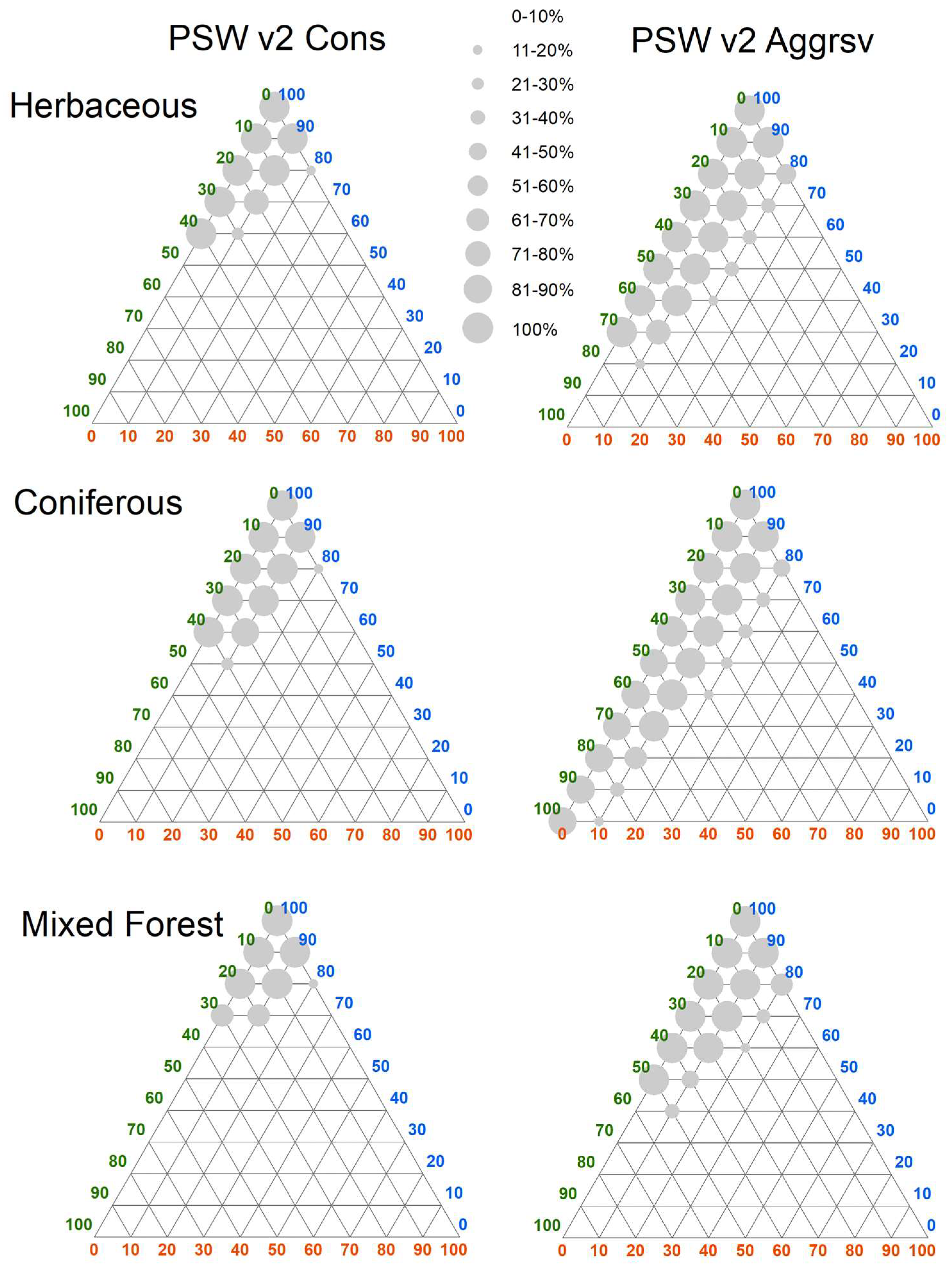
The decision rules of each test were applied to all vegetation/soil combination worksheets (Section 2.2). The ternary diagrams for every test/soil group/vegetation cover/sensor combination (n = 96) are provided as supplementary material 1 (S1). However, the results by vegetation cover type and test as lumped across soil types and sensors (n = 16 for each ternary diagram) were composited and are provided as Figure 7. For example (to aid in interpretation), in the case of herbaceous cover and PSW v2-Aggrsv (Figure 7 top row, right column): inundation was declared across all soil groups and sensors (i.e., 100%) with as little as 30% water and 70% vegetation; inundation was declared for more than 70% (but less than 80%) of the soil/sensor cases given 30% water, 60% vegetation, and 10% soil; and more than 10% (but less than 20%) when the mixture was 20% water, 70% vegetation cover and 10% bare soil—this last case being caused by slight differences in sensor response (see discussion below).
In comparison, the PSW v2-Aggrsv test only required 30 and 50% water for herbaceous and mixed forest land covers, respectively, before inundation was declared. This resulted in lower errors of omission in the Everglades study area and elsewhere as discussed subsequently. Yet, PSW v2-Aggrsv induced commission errors are clear for the coniferous forest endmember (Figure 7, middle row, right side). Obviously incorrect declarations of inundation were declared for 100% of the soil/sensor cases with 100% coniferous vegetation cover and no water. Importantly, for those same water/coniferous cover/soil spectral mixtures, PSW v2-Cons is resistant to errors of commission and is therefore the correct test to apply in environments with such canopy cover and soil conditions (left side, middle row of Figure 7). Aggressive test (PSW v2-Aggrsv) performance is discussed further in Section 3.2 and Section 3.3.
The continuity of ETM- and OLI-derived reflectance and spectral indices has been examined [49,50,51,52]. Calibration to at-surface reflectance produced variation across sensors on the order of 3 to 5% depending on calibration technique [50] and conversion to reflectance for purposes of biophysical modeling is important [49]. Differences among ETM- and OLI-derived values of NDVI and MNDWI were uncovered at low and high values, respectively [52]. As employed in the DSWE model, however, rule thresholds are at high values for NDVI and extremely low values for MNDWI, meaning they are unaffected by the differences observed in [52]. Conclusions drawn for vegetation indices using ground collected data resampled to ETM/OLI spectra [51] indicated surface reflectance spectra drawn from ETM and OLI are sufficiently correlated to afford long-term studies. Regardless, consistency as a function of sensor (TM class or OLI) was evaluated by comparing pair-wise ternary diagrams within cover/soil group combinations (N = 48).
Some caveats are appropriate. Reflectance values generated by ENVI and ArcMap were expressed to 8 significant digits. Differences between band-specific reflectance generated in the table were typically below the uncertainty reported for Landsat Surface Reflectance Products (ρ*0.05 + 0.005) [53]. As one example selected at random, herbaceous cover and the inceptisol brown to dark brown soil group, PSW v2-Cons as applied to TM does not declare inundation at 80% water cover, while it does given the OLI spectrum (these results may be seen in the S1 graphs labelled “TM_Inceptisol_Br2DBr_grass_PSW v2-Cons ” and “”OLI_ Inceptisol_Br2DBr_grass_PSW v2-Cons”). This difference was caused by the TM Band 5 value exceeding the 0.09 reflectance threshold by 3.59 × 10⁻⁵. In addition, discretization of the mixture constituents at 10% intervals may make differences in test results as a function of Landsat sensors seem unnecessarily large. For example, the difference in shortwave infrared TM Band 5 and OLI Band 6 reflectance in the aforementioned case was 4.51 × 10⁻⁴. Caveats aside, examination of the ternary diagrams (S1) showed that 31 of 48 pairings (65%) exhibit an exact match in results across sensors. Another 10 pairs differ by only one 10% mixture combination and the remaining 7 pairs with differences have only two 10% mixtures each without the same declaration result. All differences were at the “edges” of water detection for the rules. Given that DSWE will be produced from data calibrated to at-surface reflectance and recognizing this sensitivity in spectral modeling and ternary graph production, the DSWE rules are relatively robust across sensors and can be used to create a long-term record of inundation dynamics.
The dominance of large symbol sizes at vertices in Figure 7 suggests moderate variance in PSW test results as a function of soil color. However, smaller graduated circles in Figure 7 are primarily due to differences in soil color, not sensor type. These differences are minimal in the case of the conservative test (left column, Figure 7) and more apparent in the herbaceous and conifer cases (right top and middle, Figure 7). The dominantly vertical orientation of herbaceous and conifer canopies are environments where light is more likely to reach and return from the substrate surface. This may lead to a lack of uniformity in detectability across wetlands with differing soil colors given the application of just two rules (i.e., without customization as a function of soil substrate). Two factors support this approach nonetheless. First, soil is an edaphic factor that, in comparison to vegetation and other land cover, is far less likely to change substantially over large areas through time. Second, high quality information on soil color is lacking at fine spatial resolution, particularly at a global scale [54], making implementation of custom rules problematic in application. As efficient monitoring of temporal changes in inundation is the primary goal for DSWE, consistent application of the two rules suggested here has merit.
Focused on vegetated wetlands, these DSWE tests fail to detect inundation in the absence of vegetation cover even with the presence of significant percentages of water. That is, the lower right soil- and water-dominated corner of the ternary diagrams in Figure 7 are absent of detection declarations given just these two tests. This is acceptable as because other OW tests taken from the literature are used in the overall DSWE model. Documentation and evaluation of those tests is beyond the scope of this discussion. The key here as that these commonly employed OW models typically fail to detect the inundation that the DSWE PSW tests are designed for
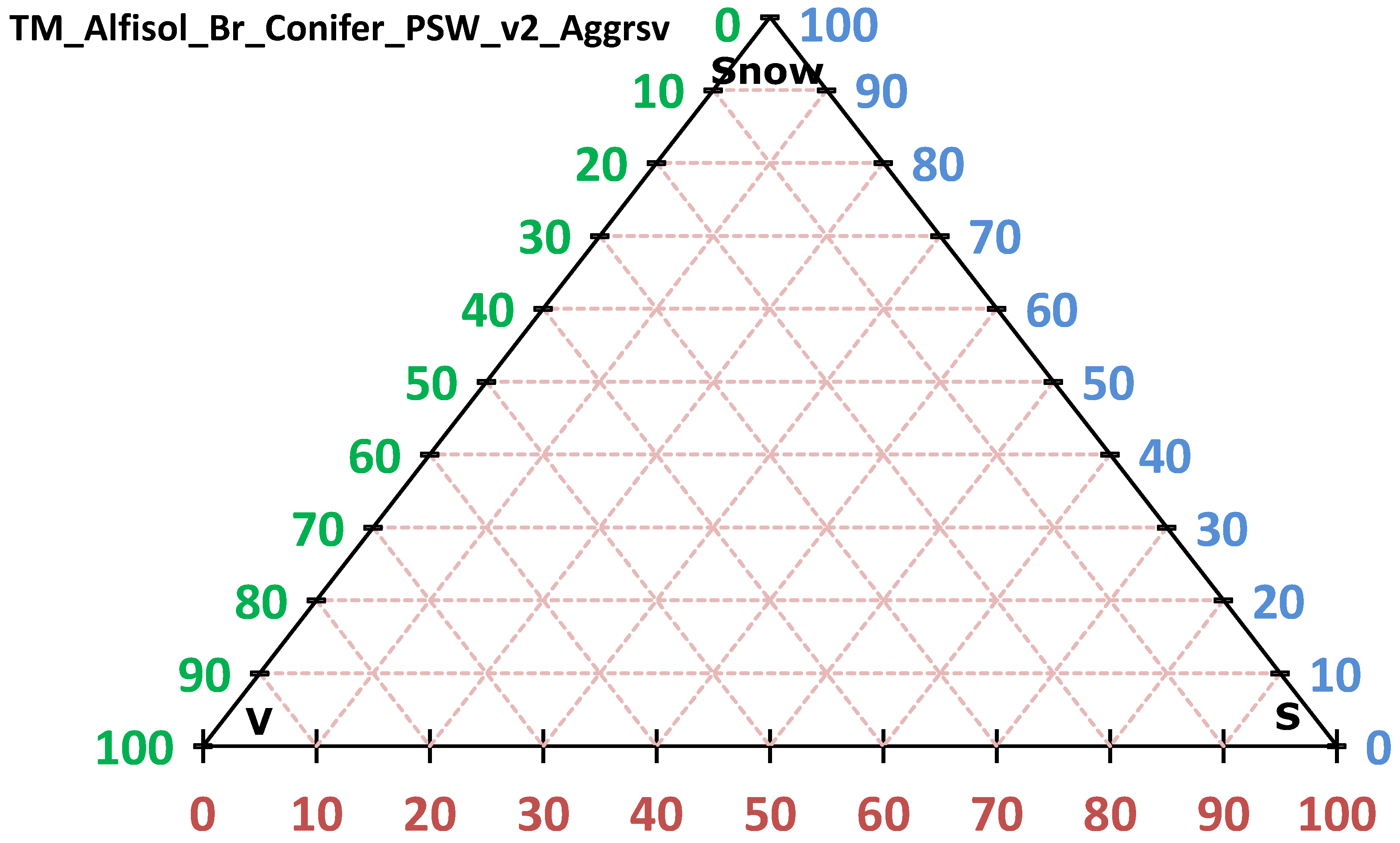
To assess whether the DSWE PSW v2 conservative or aggressive test would result in false liquid water detection (commission error) in the presence of snow cover, the average snow spectrum for each sensor (Section 2.1.5) was substituted for the water spectra in all vegetation/soil/sensor mixture models (n = 96). The ternary diagrams provided a rapid means of understanding results. Open water tests based on optical spectral indices routinely employed within the literature and used as part of the overall DSWE model confuse snow and open water. Simply stated, however, the DSWE PSW tests are insensitive to snow cover in all cases. The ternary graph shown in Figure 8 shows no declarations of “inundated” when snow is substituted for water. This graph is identical to all those from the other 95 treatments of snow, vegetation, soil, and sensor. This simulated result was supported by visual examination of validation imagery for the chips shown in Figure 1.
3.2. Everglades Point-based Analyses
All the analyses comparing DSWE PSW v2 results with Everglades in situ measured water stage were a replication of previously published experiments used to assess DSWE PSW v1 tests [4]. To allow direct comparison, both PSW v2 test outcomes were considered in combination. That is, to understand whether the PSW v2 tests are an improvement over the single PSW v1 test, each gage-based depth/L5LSRP observation was labelled “inundated” if either PSW v2-Cons or PSW v2-Aggrsv declared inundation.
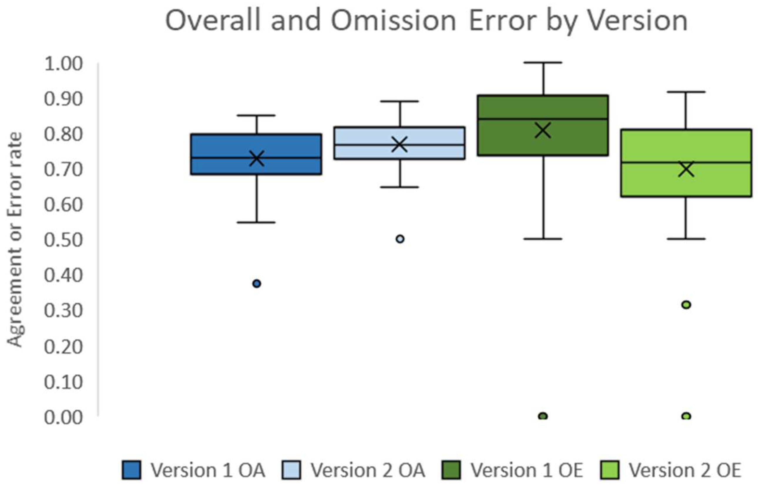
The table provided as supplementary material 2 (S2) lists the overall agreement (OA) rates, omission error (OE) rates, differences among those rates (OA Diff and OE Diff) given PSW v1 and PSW v2 tests, as well as the number of valid gages associated with each study date (N). Weather and gage operational conditions across the 50 image dates resulted in 3,736 valid observations. Table 5 and Figure 9 statistically summarize the data listed in S2 and Figure 10, Figure 11, Figure 12 and Figure 13 graphically portray the changes on a pairwise (v1 to v2) basis.
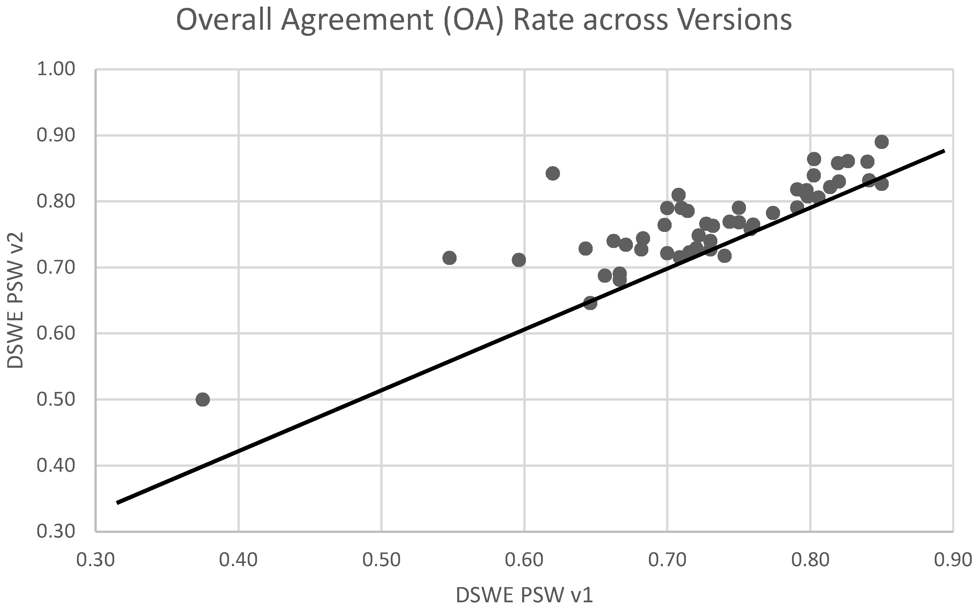
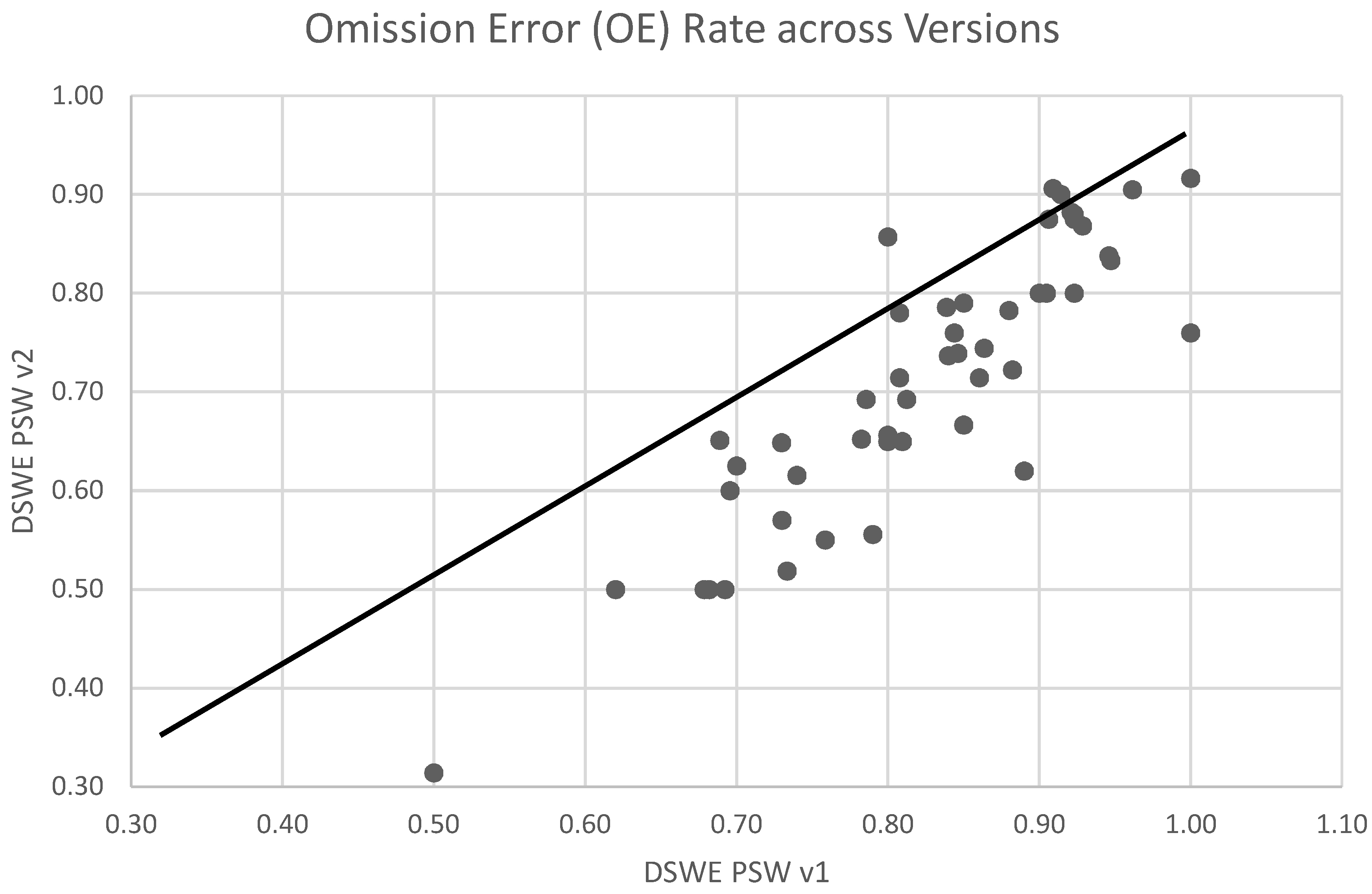
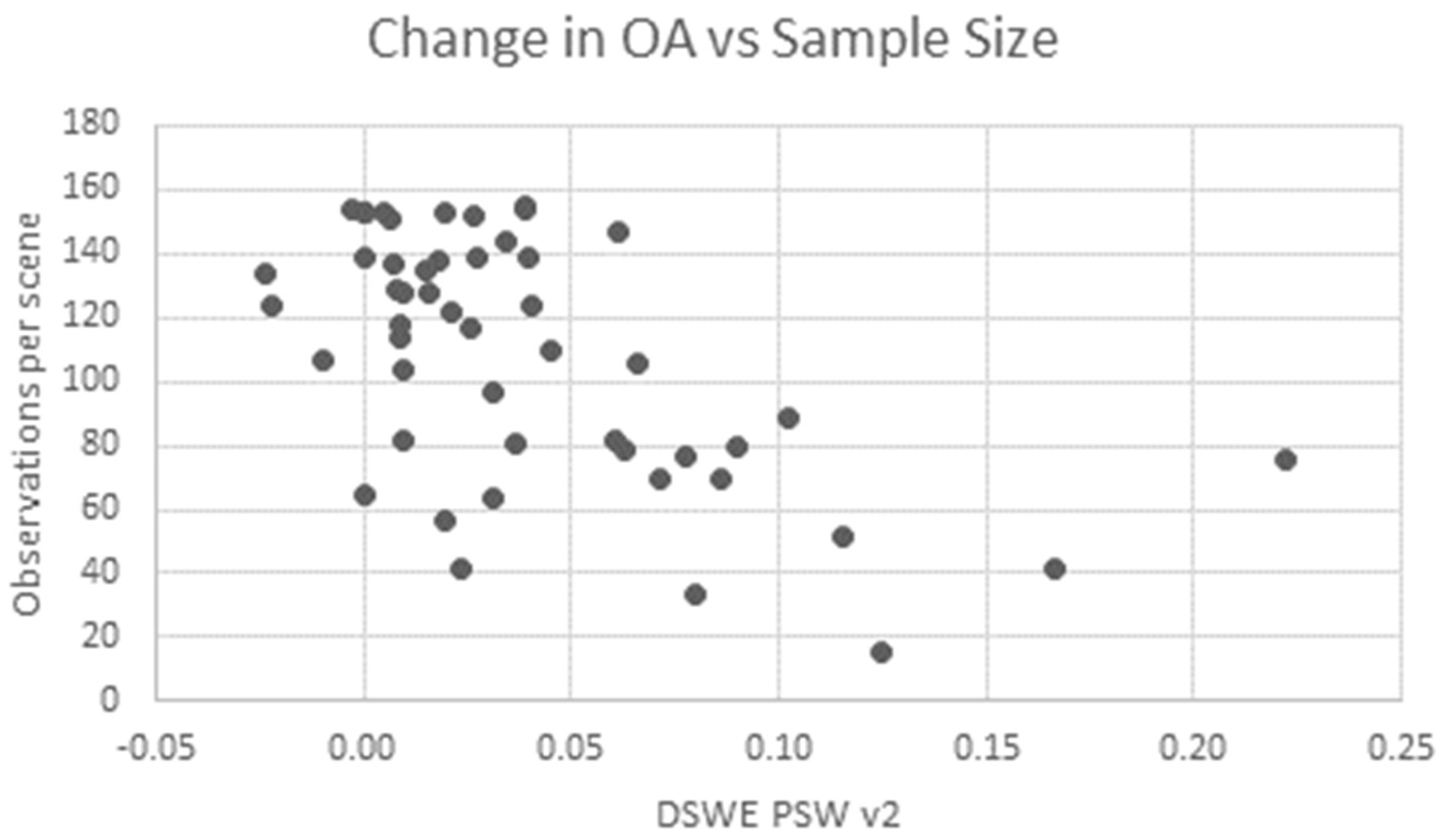
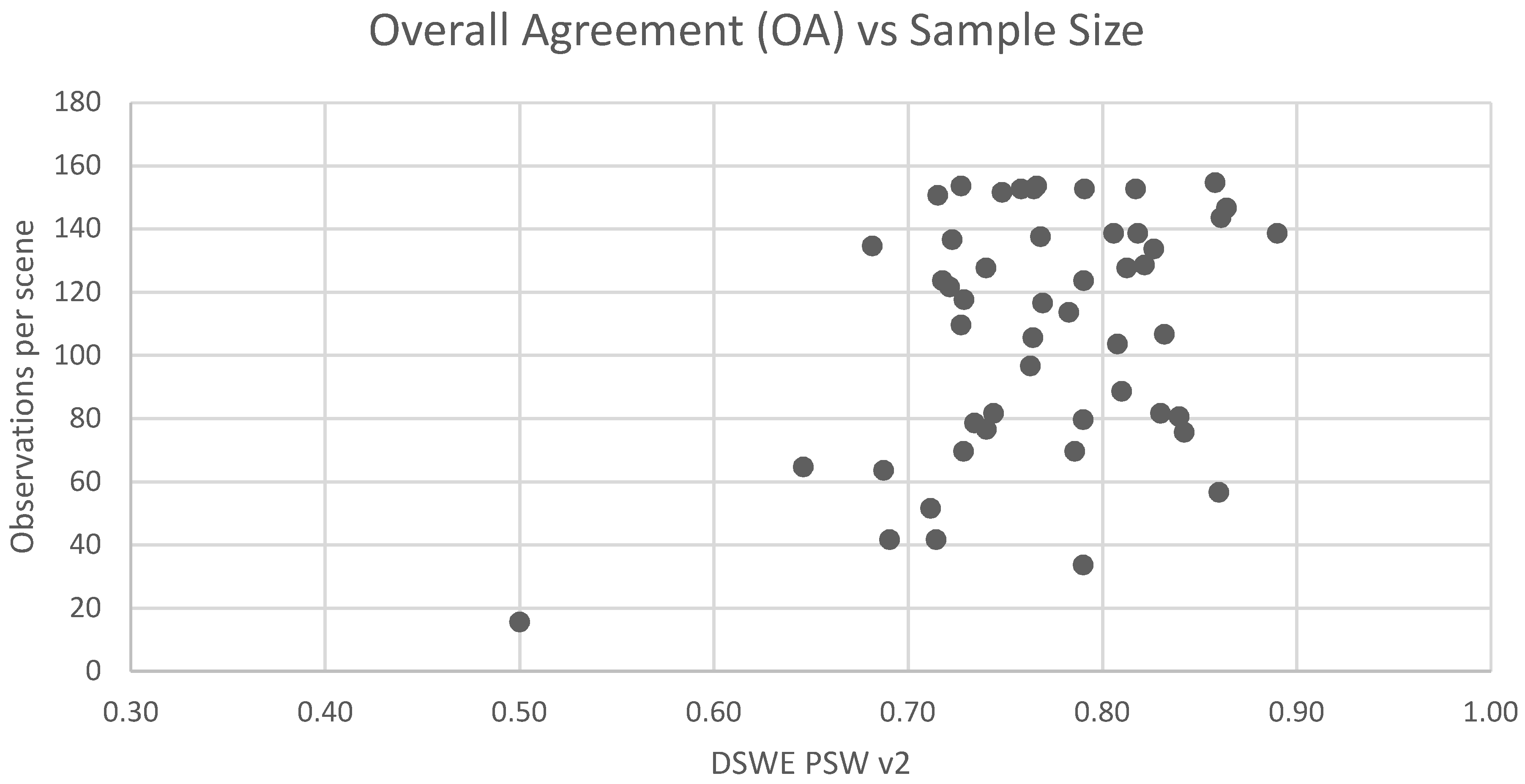
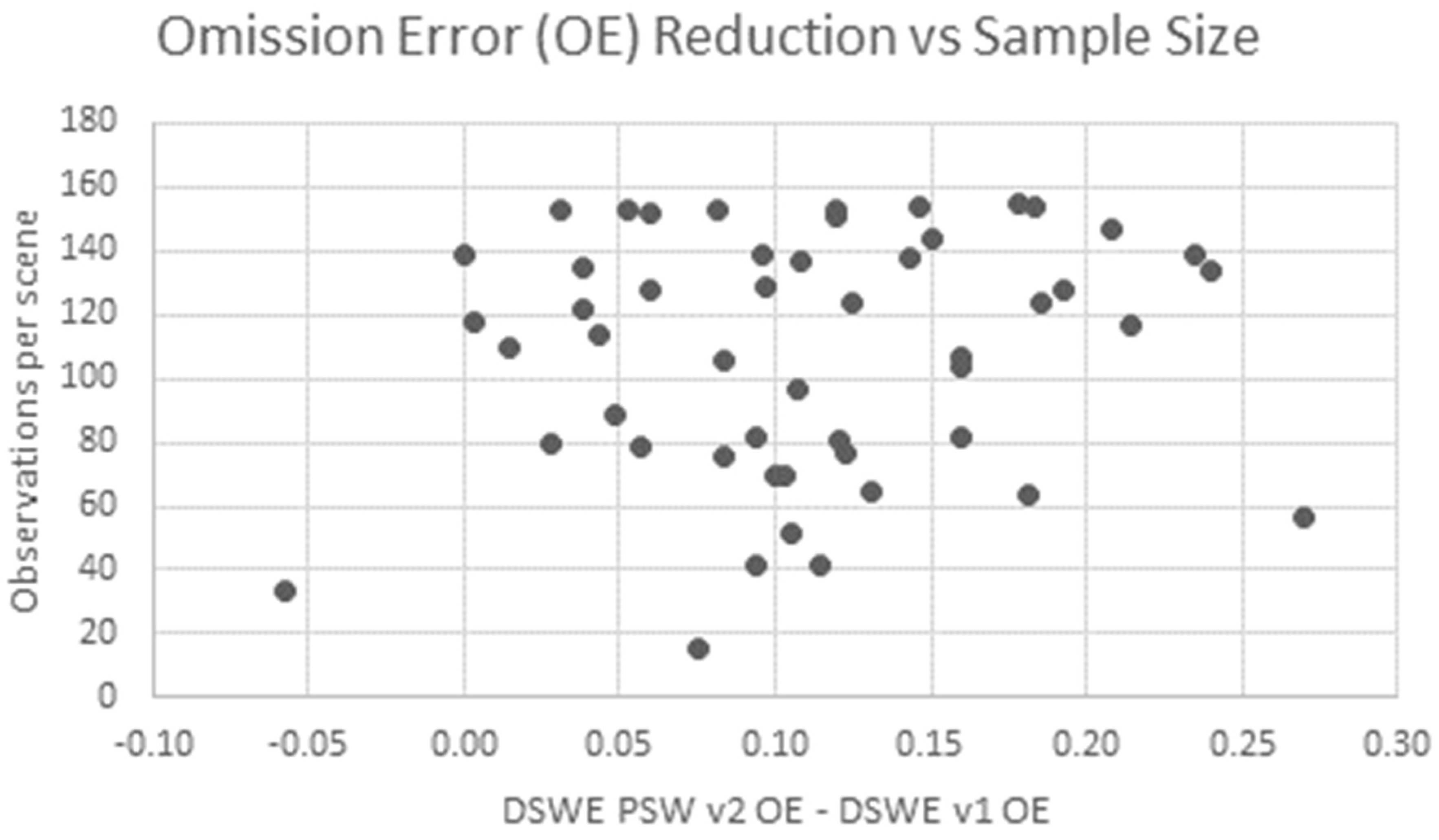
DSWE PSW v2 had an average overall agreement rate of 77% compared to v1′s average of 73%. The minimum OA agreement rate for PSW v2 (50%) was 12% higher than the equivalent measure for v2 (38%). Although 3 of the 50 scenes exhibited a decrease in OA, the maximum of that decrease was 2%. And all other measures on OA show improvement, with a statistically significant increase in mean OA (p = 0.01) given the DSWE test revisions. This increase was achieved through the desired and statistically significant (p = 0.009) average decrease in OE compared to the rate associated with DSWE PSW v1. A single exception to OE reduction (6%) was produced by the image date with the second fewest viable observations (5/9/2002, n = 34), while nonetheless improving OA 9% given the application of DSWE PSW v2 tests. It is easy to interpret the OA increase as a function of sample size (Figure 12) as simply a matter of mathematical leverage: fewer correct answers are needed to boost OA given a low total number of available observations. However, as with results for v1 [4], the relationship among OA and sample size is weak (Figure 13) and importantly, reductions in OE occurred regardless of sample size (Figure 14).
A goal of DSWE product development is to yield the highest temporal frequency information and detection capabilities possible at the pixel level regardless of overall image quality [4]. Figure 11 and Figure 14 show that some, often large improvements in OA and reductions in OE, respectively, occurred across the entire range of sample sizes. This indicates that the v2 tests not only overcome some potential interference caused by cloudy atmospheric conditions (i.e., when observations are few), they reduce omission errors in marshlands across the range of atmospheric conditions through greater sensitivity to spectral differences caused by inundation. This finding further supports the conclusion that the combined DSWE PSW v2 tests are more suitable than the PSW v1 test for building the most temporally fine time series possible from Landsat surface reflectance data.
3.3. Visual Inspection
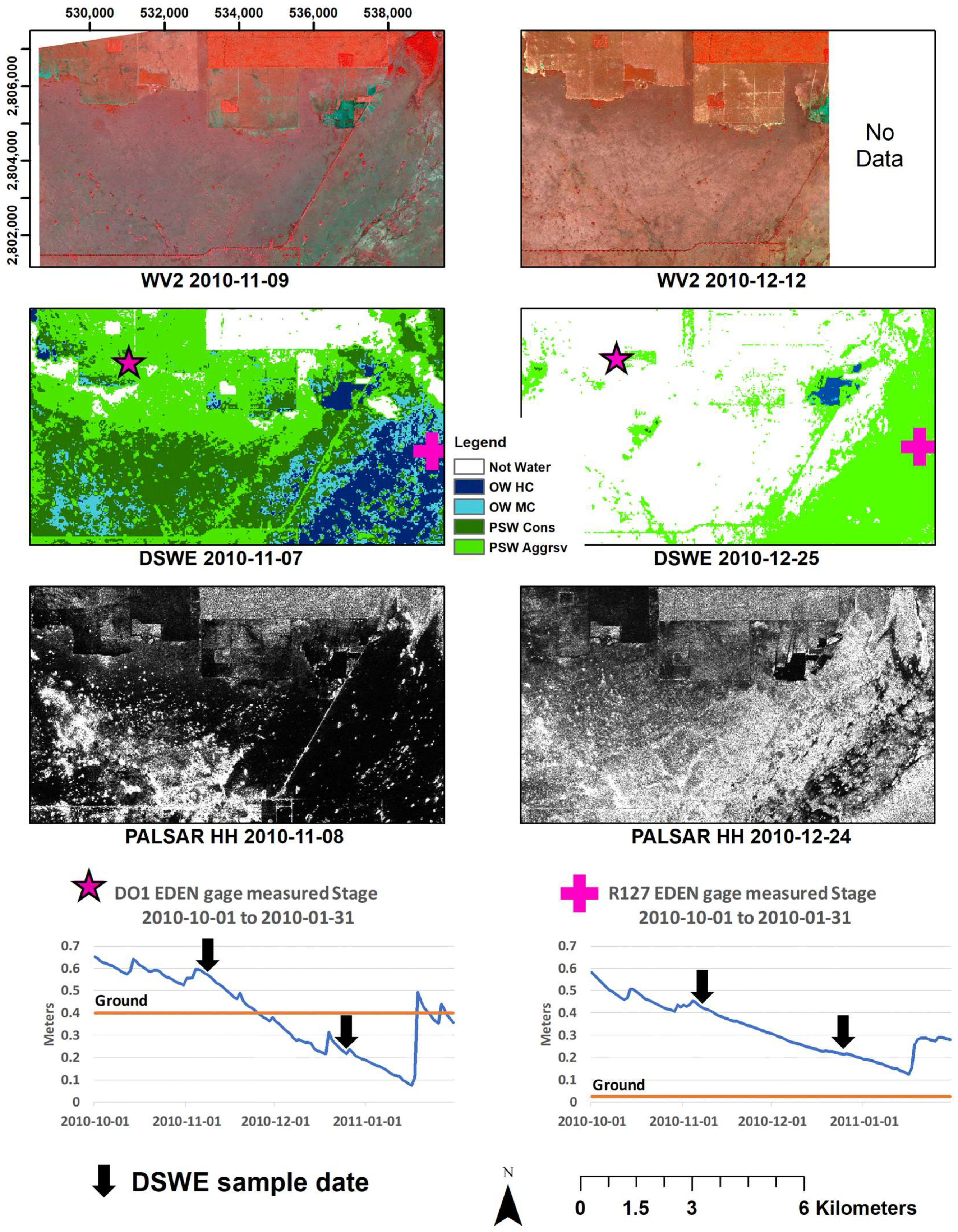
The entire DSWE model contains five tests. In addition to the two tests detailed here, three others are best suited to detecting pixels entirely composed of open water. To aid the discussion of the PSW tests, the Figures presented here depict DSWE model output in which all five tests were used. The data in Figure 15 were compiled for the subarea of chip 9 in Figure 1 directly southwest of the main entrance to the Everglades National Park. This example is indicative of the leveraging of data sources employed during DSWE evaluation and the general performance of DSWE in herbaceous wetland environments. Commercial high-resolution and openly available RADAR data collected nearly coincident with the Landsat overpasses were combined with in situ data. False color composites from Worldview 2 imagery with 2.4m ground resolution make areas of open water most apparent while variations in vegetation structure and land use at Landsat subpixel resolution may also be assessed. Advanced Land Observing Satellite (ALOS) Phased Array Synthetic Aperture Radar (PALSAR) L-band horizontal transmit/horizontal receive (HH) data with 12.5m ground resolution generally exhibit the previously documented inverse relationship between intensity and water level (and therefore inundation extent) [55]. EDEN data confirm when and where water was above ground.
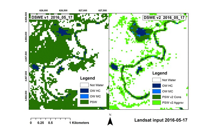
The PALSAR sigma0 data are not processed to a binary map of water extent but are instead displayed in manners that enhance spatial detail. Dark areas are ones with relatively deep water/low vegetation cover while brightest returns are caused by volume scattering in dense vegetation or rough bare water surfaces or double bounce effects with inundated shrub or very dense sawgrass [56]. Overall, temporal changes in DSWE mapped patterns of inundation are similar to patterns interpreted from the PALSAR imagery. A possible exception is in the eastern portion of the 2010-12-24 PALSAR image, along the western margin of a major slough, where the increased area of bright returns during this relatively dry period may be due to increased volume scattering. Additional vegetation rises above the water surface that has receded but is still above ground. Alternatively, bright returns may be caused by rough microtopography visible once surface water has completely receded. DSWE v2 declaration of “inundation” in these areas suggests that double-bounce increased scattering is the cause. However, that specific region of the PALSAR imagery requires further investigation before that particular issue can be resolved. DSWE accurately detects the open water clearly seen in the Worldview scenes. DSWE declarations of inundation match EDEN gage inundation state, the most defensible “ground truth” available. Importantly, given the dominance of PSW classes in the Everglades, without a PSW component, DSWE would fail to detect most of the inundation dynamics in the Everglades.
Figure 16 shows DSWE v1 and v2 output generated from the same Landsat input for chip 60 (Figure 1), a conterminous US location that is nearly as far away from the Everglades (chip 9, Figure 1) as is possible. In addition, the location in Figure 16 has a very different physiography, climate, and land cover than the Everglades. This area of Oregon contains rugged terrain, coniferous forests, and wide-ranging water/vegetation substrates - including lava flows. The high rate of commission errors in coniferous environments that result from DSWE v1 are evident (upper left, Figure 16). The reduction of commission errors by both PSW v2 tests and their representation as separate DSWE classes are also clear (upper right, Figure 16). Inundation detected by the DSWE conservative test (PSW v2-Cons) coincides with dark regions in the RADARSAT-2 C-band HH sigma0 data (lower right, Figure 16). Small errors of commission remain where there are slight breaks in terrain and along small roadways – where tall forest canopies shade the narrow road features below. Errors from these sources are exacerbated by lower sun angle conditions. Note that the lava field visible in the east-central portion of U.S. Department of Agriculture (USDA) orthophotography (lower left pane, Figure 16) and as high RADAR return due to volume scattering of the very rough surface (lower right pane, Figure 16), which might prove a source of confusion for some OW classifiers, is not declared inundated by either version of the DSWE model.
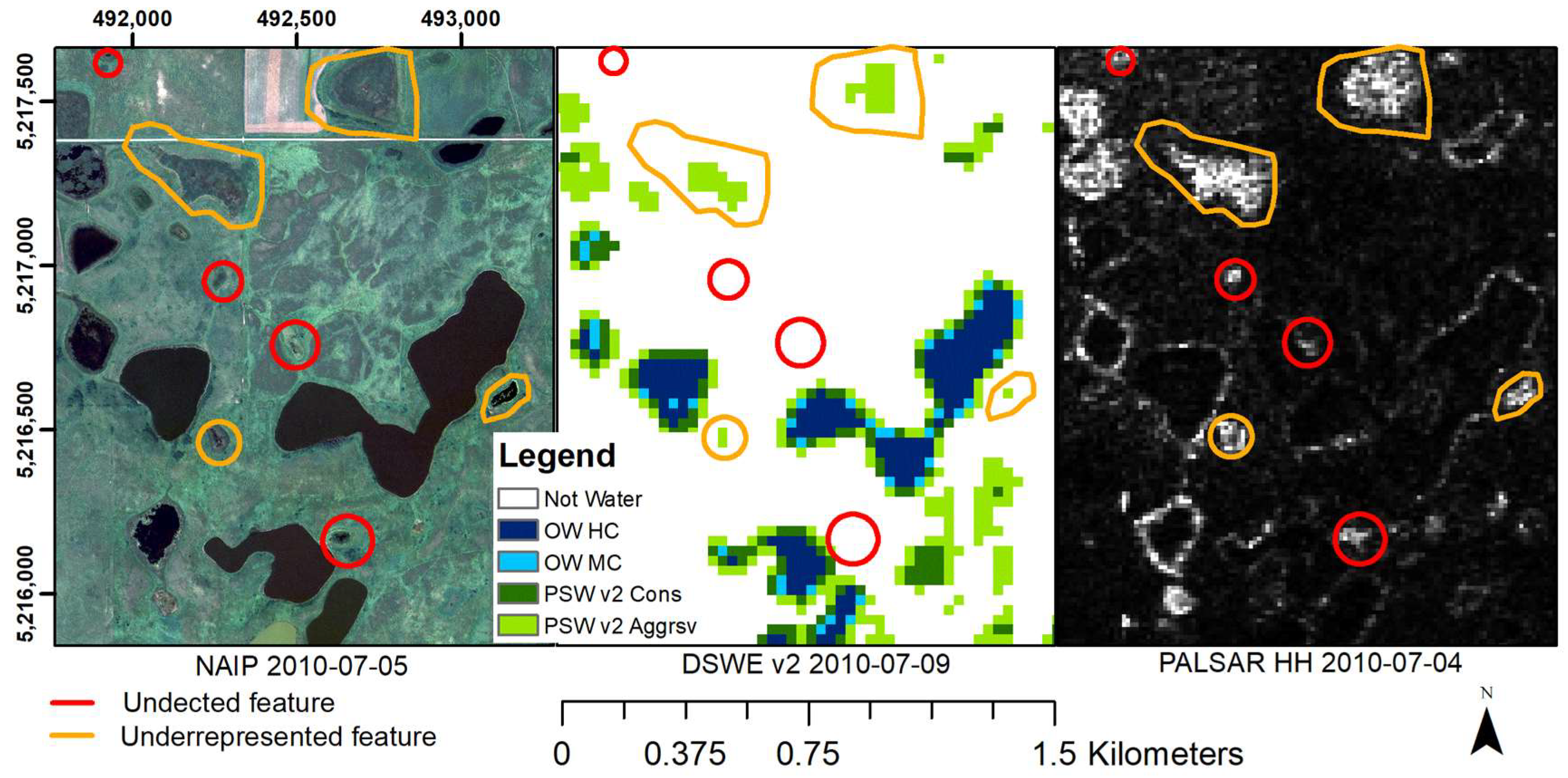
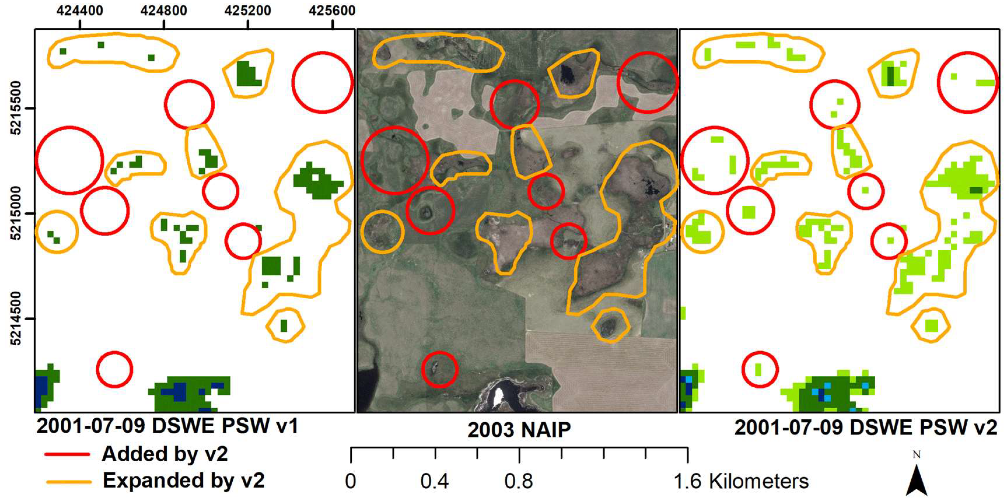
Chip 36 in Figure 1 is located in the prairie pothole region of North America, a critical migratory bird flyway and region important for carbon and methane cycling [57,58]. Figure 17 includes 1m spatial resolution USDA orthophotography and 12.5m spatial resolution L-band PALSAR imagery that were collected one day apart. The Landsat imagery used to generate DSWE v2 output shown was collected 4 days after the air photos and 5 days after the SAR imagery. In this case, double-bounce effects on intensity are evident and correspond closely with the presence of DSWE PSW v2-Aggrsv (aggressive test 2) distribution. Specifically, ringing caused by bright double bounce returns surrounding large water features or throughout smaller ones match the locations of PSW v2-Aggrsv detections of surface water. This is additional evidence that the aggressive test is representing mixed pixels of water and vegetation. Limits on DSWE resolution are also evident in this imagery. Red colored circles identify likely inundated features entirely missed by DSWE v2. The southern-most red circle in the images surrounds the largest feature not detected by DSWE v2 given this Landsat scene. The feature measures approximately 50m by 40m along its major axis. Orange outlined areas highlight features detected by DSWE that are not as fully represented as might be possible with higher spatial resolution data. Nonetheless, inundation mapping approaches best suited for open water detection would fail to detect many sizable features and under-represent the size of others to an even greater degree than the DSWE PSW tests both here and in other environments.
Another subset from the prairie pothole region (i.e., chip 36 in Figure 1) is shown in Figure 18. In this case, DSWE v1 and v2 output generated from the same input Landsat image are displayed. By design, DSWE can be derived from any at-surface reflectance data created from Landsat TM or newer instruments. This means DSWE data can potentially be produced for periods as early as some time in 1984. The date of the Landsat source imagery shown in Figure 18 is 9 July 2001. This image/date was selected through the examination of nearly 1000 DSWE maps for this chip that were embedded in an animation as part of on-going experiments in DSWE visualization. It was chosen for the moderate inundation conditions present at the time, representing neither drought nor flood conditions, as well as relatively clear atmospheric conditions. Higher spatial resolution images that can be effectively used for DSWE assessment are difficult to acquire for dates prior to the mid-2000s, when high fidelity digital airborne cameras systems became more widespread and US Federal programs facilitated bi-annual and in some places annual digital orthophotograph production. In contrast to the near-coincident, independent inundation data sources used in all other examples, the orthophotograph used for Figure 18 differs in time by several years from that of the Landsat input to DSWE and is provided only as a general visual guide for wetland feature identification.
Figure 18 reinforces the improvement in subpixel inundation detection afforded by the revised DSWE PSW tests, that is, both PSW v2-Cons and PSW v2-Aggrsv. Through this comparison, the decreased errors of omission sought through DSWE PSW v2 test development are again evident. In contrast to Figure 17, features circled in red represent those that were not detected by the DSWE PSW v1 test. Those features surrounded by orange vectors are ones for which far greater inundation and corresponding shape characteristics have been detected and delineated by the DSWE PSW v2 tests.
Figure 19 illustrates an example of DSWE-generated information potential for resource management. The DSWE data in the right figure pane is the same (17 May 2016) v2 output used for Figure 16. In this case, however, the data were clipped to a boundary of potential amphibian habitat [59], shown as a black vector, to eliminate areas outside the possible amphibian range. On 9 September 2001 (left), mean discharge for the Deschutes River, Oregon, as measured upstream at USGS station number 14056500 [60], was 19.94 cubic meters per second (m3s−1). For May 18 (right side) mean daily flow was higher (28.88 m3s). Despite large differences in contributing streamflow, the largest and a moderately sized wetland are not inundated in September, while others of moderate and small size were inundated on both dates. DSWE can be used to quickly generate hundreds of observations from the Landsat Archive that can be compiled to assess wetland feature inundation trends, connectivity, and function.
The Deschutes River is roughly 50m wide in this area. Without the capacity to detect inundation at the subpixel level, that is for example the PSW components of DSWE, the Deschutes would not be detected. In other words, DSWE is able to provide data on reaches and wetlands that would be undetected by open water indices alone. Of critical importance to habitat monitoring on-the-whole, the DSWE model’s ability to detect inundation patterns in vegetated areas provides a critical, optical sensor-based record for amphibian and aquatic species habitat management.
4. Conclusions and Future Research
This research focused on the development and evaluation of Landsat-based tests for the detection of inundation when pixels are partially covered by water and vegetation, places where algorithms designed to detect open surface water using Landsat typically perform inadequately [4,5]. A robust approach was developed to revise and improve DSWE decision rules for that purpose. In combination, revised DSWE PSW tests demonstrated improved overall accuracy with a desired reduction in errors of omission based on quantitative analyses of in situ data from the Everglades, Florida. Visual comparison of DSWE output with nearly coincident imagery reflects improvements made in the Everglades, for locations across the US.
For science and resource management applications in which the importance of detecting small areas of inundation and monitoring their dynamics is paramount, commission errors are preferable over omission errors. DSWE PSW tests are resistant to commission error caused by snow cover. However, the open water tests employed in DSWE are not. Users should expect higher commission error for Landsat imagery collected where topography, tree cover, or infrastructure cast shadows, where coniferous or thick mixed forest canopies are present, and during times when sun angles are low. In practice, DSWE model application requires DEM data inputs so that derived slope and hillshade layers may be used to mitigate commission errors over steep slopes and in terrain shadows. Cloud, cloud-shadow, and snow masks derived from the quality data provided with the Landsat input to DSWE [36,37] demark other areas where DSWE model output for a particular Landsat overpass date are not reliable.
Detectability varies slightly as a function of soil substrate. However, DSWE-based measurements of inundation for a given location will retain stationarity as a function of soil type because edaphic factors generally change at a lower frequency than vegetation or land uses above them. Differences in model responses are greater as a function of land cover. While one might suggest that a separate test be created for each vegetation cover type, conversion from one type or condition to another due to natural disturbance or anthropogenic change occurs at higher temporal frequencies than are currently systematically recorded through land cover mapping – particularly at a global scale. The DSWE model will be applied over a 34-year (and growing) timeframe. The high-resolution temporal and spatial land cover data needed to guide test application as a function of land cover type are currently lacking. Therefore, uniform DSWE tests applied without scene-specific training data is an efficient and effective approach to generating useful and currently unavailable inundation dynamics information over large areas and extended time periods, with high spatial resolution and temporal frequency.
Data Availability
All input data employed for this research are publicly available. The Landsat Archive repository may be obtained through https://earthexplorer.usgs.gov/. USGS streamflow data is available through https://waterdata.usgs.gov/nwis. And the EDEN gage data may be obtained via https://sofia.usgs.gov/eden/.
Supplementary Materials
The following are available online at https://www.mdpi.com/2072-4292/11/4/374/s1, An Adobe Acrobat document (named S1.pdf) containing ternary graphs for the mixture model results produced by every water, soil, vegetation, and sensor combination, and a Microsoft Word file (named S2.docx) containing a table that provides the error and accuracy statistics on DSWE partial surface water tests versions 1 and 2 for every study scene.
Author Contributions
The author was solely responsible for the conceptualization and development of DSWE; the research presented in this manuscript; and the composition of this manuscript. The ternary diagram processing assistance provided by Coral Roig-Silva is attributed in the acknowledgements section.
Funding
This research was supported by the USGS Land Remote Sensing Program.
Acknowledgments
The author gratefully acknowledges establishment of an Excel ternary diagram template by Coral Roig-Silva. Worldview 2 data were provided by DigitalGlobe through the NGA NextView contract. Alos PALSAR data were provided by the Americas ALOS Data Node (AADN) located at the Alaskan Satellite Facility (ASF). Any use of trade, firm, or product names is for descriptive purposes only and does not imply endorsement by the U.S. Government.
Conflicts of Interest
The author declares no conflict of interest.
References
- Loveland, T.R.; Dwyer, J.L. Landsat: Building a strong future. Remote Sens. Environ. 2012, 122, 22–29. [Google Scholar] [CrossRef]
- Australia, G. Water Observations from Space. Available online: http://www.ga.gov.au/scientific-topics/hazards/flood/wofs (accessed on 5 September 2018).
- Pekel, J.-F.; Cottam, A.; Gorelick, N.; Belward, A.S. High-resolution mapping of global surface water and its long-term changes. Nature 2016, 540, 418–422. [Google Scholar] [CrossRef] [PubMed]
- Jones, J.W. Efficient Wetland Surface Water Detection and Monitoring via Landsat: Comparison with in situ Data from the Everglades Depth Estimation Network. Remote Sens. 2015, 7, 12503–12538. [Google Scholar] [CrossRef] [Green Version]
- Devries, B.; Huang, C.; Lang, M.W.; Jones, J.W.; Creed, I.F.; Carroll, M.L. Automated Quantification of Surface Water Inundation in Wetlands Using Optical Satellite Imagery. Remote Sens. 2017, 9, 807. [Google Scholar] [CrossRef]
- Carroll, M.L.; Loboda, T.V. Multi-Decadal Surface Water Dynamics in North American Tundra. Remote Sens. 2017, 9, 497. [Google Scholar] [CrossRef]
- Bjerklie, D.M.; Birkett, C.M.; Jones, J.W.; Carabajal, C.; Rover, J.A.; Fulton, J.W.; Garambois, P.-A. Satellite remote sensing estimation of river discharge: Application to the Yukon River Alaska. J. Hydrol. 2018, 561, 1000–1018. [Google Scholar] [CrossRef]
- Huang, W.; Devries, B.; Huang, C.; Lang, M.W.; Jones, J.W.; Creed, I.F.; Carroll, M.L. Automated Extraction of Surface Water Extent from Sentinel-1 Data. Remote Sens. 2018, 10, 797. [Google Scholar] [CrossRef]
- Huang, C.; Chen, Y.; Zhang, S.; Wu, J. Detecting, Extracting, and Monitoring Surface Water From Space Using Optical Sensors: A Review. Rev. Geophys. 2018, 56, 333–360. [Google Scholar] [CrossRef]
- Ozesmi, S.L.; Bauer, M.E. Satellite remote sensing of wetlands. Wetlands Ecol. Manage. 2002, 10, 381–402. [Google Scholar] [CrossRef]
- Rover, J.; Wylie, B.K.; Ji, L. A self-trained classification technique for producing 30 m percent-water maps from Landsat data. Int. J. Remote Sens. 2010, 31, 2197–2203. [Google Scholar] [CrossRef]
- Frohn, R.C.; D’Amico, E.; Lane, C.; Autrey, B.; Rhodus, J.; Liu, H. Multi-temporal sub-pixel landsat ETM+ classification of isolated wetlands in cuyahoga county, OHIO, USA. Wetlands 2012, 32, 289–299. [Google Scholar] [CrossRef]
- Huang, C.; Peng, Y.; Lang, M.; Yeo, I.-Y.; Mccarty, G. Wetland inundation mapping and change monitoring using Landsat and airborne LiDAR data. Remote Sens. Environ. 2014, 141, 231–242. [Google Scholar] [CrossRef]
- Adams, J.B.; Smith, M.O.; Johnson, P.E. Spectral mixture modeling: A new analysis of rock and soil types at the Viking Lander 1 Site. J. Geophys. Res. 1986, 91, 8098. [Google Scholar] [CrossRef]
- Shanmugam, P.; Ahn, Y.-H.; Sanjeevi, S. A comparison of the classification of wetland characteristics by linear spectral mixture modelling and traditional hard classifiers on multispectral remotely sensed imagery in southern India. Ecol. Model. 2006, 194, 379–394. [Google Scholar] [CrossRef]
- Melendez-Pastor, I.; Navarro-Pedreño, J.; Gómez, I.; Koch, M. Detecting drought induced environmental changes in a Mediterranean wetland by remote sensing. Appl. Geogr. 2010, 30, 254–262. [Google Scholar] [CrossRef]
- Schmid, T.; Gumuzzio, J.; Koch, M. Multisensor approach to determine changes of wetland characteristics in semiarid environments (central Spain). IEEE Trans. Geosci. Remote Sens. 2005, 43, 2516–2525. [Google Scholar] [CrossRef]
- Cui, T.; Gong, Z.; Zhao, W.; Zhao, Y.; Lin, C. Research on estimating wetland vegetation abundance based on spectral mixture analysis with different endmember model: a case study in Wild Duck Lake wetland, Beijing. Acta Ecol. Sin. 2013, 33, 1160–1171. [Google Scholar]
- He, M.; Zhao, B.; Ouyang, Z.; Yan, Y.; Li, B. Linear spectral mixture analysis of Landsat TM data for monitoring invasive exotic plants in estuarine wetlands. Int. J. Remote Sens. 2010, 31, 4319–4333. [Google Scholar] [CrossRef]
- Rogers, A.S.; Kearney, M.S. Reducing signature variability in unmixing coastal marsh Thematic Mapper scenes using spectral indices. Int. J. Remote Sens. 2004, 25, 2317–2335. [Google Scholar] [CrossRef]
- Halabisky, M.; Moskal, L.M.; Gillespie, A.; Hannam, M. Reconstructing semi-arid wetland surface water dynamics through spectral mixture analysis of a time series of Landsat satellite images (1984–2011). Remote Sens. Environ. 2016, 177, 171–183. [Google Scholar] [CrossRef] [Green Version]
- Xia, H.; Zhao, W.; Li, A.; Bian, J.; Zhang, Z. Subpixel Inundation Mapping Using Landsat-8 OLI and UAV Data for a Wetland Region on the Zoige Plateau, China. Remote Sens. 2017, 9, 31. [Google Scholar] [CrossRef]
- Robertson, L.D.; King, D.J.; Davies, C. Assessing Land Cover Change and Anthropogenic Disturbance in Wetlands Using Vegetation Fractions Derived from Landsat 5 TM Imagery (1984–2010). Wetlands 2015, 35, 1077–1091. [Google Scholar] [CrossRef]
- Brivio, P.A.; Zilioli, E. Assessing wetland changes in the venice lagoon by means of satellite remote sensing data. J. Coast. Conserv. 1996, 2, 23–32. [Google Scholar] [CrossRef]
- Sun, W.; Du, B.; Xiong, S. Quantifying Sub-Pixel Surface Water Coverage in Urban Environments Using Low-Albedo Fraction from Landsat Imagery. Remote Sens. 2017, 9, 428. [Google Scholar] [CrossRef]
- Xiong, L.; Deng, R.; Li, J.; Liu, X.; Qin, Y.; Liang, Y.; Liu, Y. Subpixel Surface Water Extraction (SSWE) Using Landsat 8 OLI Data. Water 2018, 10, 653. [Google Scholar] [CrossRef]
- Adams, J.B.; Gillespie, A.R. Remote Sensing of Landscapes with Spectral Images: A Physical Modeling Approach; Cambridge University Press: New York, NY, USA, 2006; pp. 1–362. [Google Scholar]
- Shi, C.; Wang, L. Incorporating spatial information in spectral unmixing: A review. Remote Sens. Environ. 2014, 149, 70–87. [Google Scholar] [CrossRef]
- Elmore, A.J.; Mustard, J.F.; Manning, S.J.; Lobell, D.B. Quantifying Vegetation Change in Semiarid Environments: Precision and Accuracy of Spectral Mixture Analysis and the Normalized Difference Vegetation Index. Remote Sens. Environ. 2000, 73, 87–102. [Google Scholar] [CrossRef]
- Small, C. The Landsat ETM+ spectral mixing space. Remote Sens. Environ. 2004, 93, 1–17. [Google Scholar] [CrossRef]
- Ji, L.; Zhang, L.; Wylie, B. Analysis of Dynamic Thresholds for the Normalized Difference Water Index. Photogramm. Eng. Remote Sens. 2009, 75, 1307–1317. [Google Scholar] [CrossRef]
- Jones, J.W. Remote Sensing of Vegetation Pattern and Condition to Monitor Changes in Everglades Biogeochemistry. Crit. Rev. Environ. Sci. Technol. 2011, 41, 64–91. [Google Scholar] [CrossRef]
- Sousa, D.; Small, C. Global cross-calibration of Landsat spectral mixture models. Remote Sens. Environ. 2017, 192, 139–149. [Google Scholar] [CrossRef] [Green Version]
- Baldridge, A.; Hook, S.; Grove, C.; Rivera, G. The ASTER spectral library version 2.0. Remote Sens. Environ. 2009, 113, 711–715. [Google Scholar] [CrossRef]
- Small, C.; Milesi, C. Multi-scale standardized spectral mixture models. Remote Sens. Environ. 2013, 136, 442–454. [Google Scholar] [CrossRef]
- USGS. LANDSAT 4-7 Surface Reflectance (LEDAPS) Product; USGS: Sioux Falls, SD, USA, 2018; p. 38.
- USGS. LANDSAT 8 Surface Reflectance Code (LASRC) Product; USGS: Sioux Falls, SD, USA, 2018; p. 40.
- Pearlstine, L.; Smith, S.; Brandt, L.; Allen, C.; Kitchens, W.; Stenberg, J. Assessing state-wide biodiversity in the Florida Gap analysis project. J. Environ. Manage. 2002, 66, 127–144. [Google Scholar] [CrossRef] [Green Version]
- Gergely, K.J.; McKerrow, A. Terrestrial ecosystems: national inventory of vegetation and land use; US Geological Survey: Sioux Falls, SD, USA, 2013.
- Tucker, C.J. Red and photographic infrared linear combinations for monitoring vegetation. Remote Sens. Environ. 1979, 8, 127–150. [Google Scholar] [CrossRef] [Green Version]
- USGS. What are Landsat7 SLC-off Masks? Available online: https://landsat.usgs.gov/what-are-landsat-7-slc-gap-mask-files (accessed on 2 October 2018).
- Kokaly, R.F.; Clark, R.N.; Swayze, G.A.; Livo, K.E.; Hoefen, T.M.; Pearson, N.C.; Wise, R.A.; Benzel, W.M.; Lowers, H.A.; Driscoll, R.L.; et al. USGS Spectral Library Version 7, in Data Series 2017; U.S. Geological Survey Data Series 1035; U.S. Geological Survey: Reston, VA, USA, 2017; p. 61.
- Xu, H. Modification of normalised difference water index (NDWI) to enhance open water features in remotely sensed imagery. Int. J. Remote Sens. 2006, 27, 3025–3033. [Google Scholar] [CrossRef]
- Soil Survey Staff. Soil Taxonomy: A Basic System of Soil Classification for Making and Interpreting Soil Surveys, 2nd ed.; Natural Resources Conservation Service. U.S. Department of Agriculture Handbook 436; USDA: Washington, DC, USA, 1999.
- Jones, J.W.; Price, S.D. Conceptual Design of the Everglades Depth Estimation Network (EDEN) Grid; U.S. Geological Survey: Reston, VA, USA, 2007; p. 20.
- Telis, P. The Everglades Depth Estimation Network (EDEN) for Support of Ecological and Biological Assessments; U.S. Geological Survey: Reston, VA, USA, 2006.
- USGS. South Florida Information Access. 2018. Available online: http://sofia.usgs.gov (accessed on 5 September 2018).
- USGS. EDEN Gage Ancillary Data Collection Protocol. 2015. Available online: http://sofia.usgs.gov/eden/geprotocol.php (accessed on 5 May 2015).
- Flood, N. Continuity of reflectance data between landsat-7 ETM+ and landsat-8 OLI, for both top-of-atmosphere and surface reflectance: A study in the australian landscape. Remote Sens. 2014, 6, 7952–7970. [Google Scholar] [CrossRef]
- Mishra, N.; Haque, M.O.; Leigh, L.; Aaron, D.; Helder, D.; Markham, B. Radiometric Cross Calibration of Landsat 8 Operational Land Imager (OLI) and Landsat 7 Enhanced Thematic Mapper Plus (ETM+). Remote Sens. 2014, 6, 12619–12638. [Google Scholar] [CrossRef] [Green Version]
- She, X.; Zhang, L.; Cen, Y.; Wu, T.; Huang, C.; Baig, M.H.A. Comparison of the Continuity of Vegetation Indices Derived from Landsat 8 OLI and Landsat 7 ETM+ Data among Different Vegetation Types. Remote Sens. 2015, 7, 13485–13506. [Google Scholar] [CrossRef] [Green Version]
- Li, P.; Jiang, L.; Feng, Z. Cross-Comparison of Vegetation Indices Derived from Landsat-7 Enhanced Thematic Mapper Plus (ETM+) and Landsat-8 Operational Land Imager (OLI) Sensors. Remote Sens. 2014, 6, 310–329. [Google Scholar] [CrossRef]
- Claverie, M.; Vermote, E.F.; Franch, B.; Masek, J.G. Evaluation of the Landsat-5 TM and Landsat-7 ETM+ surface reflectance products. Remote Sens. Environ. 2015, 169, 390–403. [Google Scholar] [CrossRef]
- FAO; ITPS. Status of the World’s Soil Resources (SWSR)—Main Report; Nachtergaele, F., Ed.; FAO: Rome, Italy, 2015; p. 648. [Google Scholar]
- Kim, J.-W.; Lu, Z.; Jones, J.W.; Shum, C.; Lee, H.; Jia, Y. Monitoring Everglades freshwater marsh water level using L-band synthetic aperture radar backscatter. Remote Sens. Environ. 2014, 150, 66–81. [Google Scholar] [CrossRef]
- Tsyganskaya, V.; Martinis, S.; Marzahn, P.; Ludwig, R. SAR-based detection of flooded vegetation—A review of characteristics and approaches. Int. J. Remote Sens. 2018, 39, 2255–2293. [Google Scholar] [CrossRef]
- Johnson, W.C.; Millett, B.V.; Gilmanov, T.; Voldseth, R.A.; Guntenspergen, G.R.; Naugle, D.E. Vulnerability of Northern Prairie Wetlands to Climate Change. BioScience 2005, 55, 863. [Google Scholar] [CrossRef] [Green Version]
- Winter, T.C.; Rosenberry, D.O. Hydrology of Prairie Pothole Wetlands during Drought and Deluge: A 17-Year Study of the Cottonwood Lake Wetland Complex in North Dakota in the Perspective of Longer Term Measured and Proxy Hydrological Records. Clim. Change 1998, 40, 189–209. [Google Scholar] [CrossRef]
- Duarte, A. US Fish and Wildlife Habitat Conservation Planning Polygon; USFWS: Bend, OR, USA, 2018. [Google Scholar]
- USGS. USGS 14056500 Deschutes R BL Wickiup Res NR LA Pine, Oreg. 2018. Available online: https://waterdata.usgs.gov/or/nwis/nwismap/?site_no=14056500&agency_cd=USGS (accessed on 11 October 2018).
Figure 1.
The Landsat World Reference System-2 WRS-2 tile locations (chips) selected to provide broad ranges of climate, physiographic, land use, and hydrologic environments for use in DSWE model development and revision.
Figure 1.
The Landsat World Reference System-2 WRS-2 tile locations (chips) selected to provide broad ranges of climate, physiographic, land use, and hydrologic environments for use in DSWE model development and revision.

Figure 2.
ETM and OLI spectra for 8 soil groups as resampled from ASTER library spectra. Legend entries are linked to soil spectra through Table 1. (Note that at the spectral resolution of TM and OLI and the scale of these figures, the spectra for Alfisol Brown (“Alfisol_Br”) and Utisol Brown to Dark Brown (“Utisol Br2Dbr) are undistinguishable).

Figure 3.
Flow chart depicting the ETM and OLI vegetation spectra sampling process that is repeated for every band/sensor/vegetation type combination. Inputs are the Landsat Surface Reflectance Product (LSRP) bands; Gap Analysis Program (GAP) land cover; and the QA band for masking Landsat 7 missing data; and the normalized difference vegetation index (NDVI) calculated from the LSRP data. Final single band values are combined to form the given spectral endmember.

Figure 4.
ETM and OLI spectra for the vegetation classes listed in Table 2 as derived through the process depicted in Figure 3 and described in Section 2.1.4.
Figure 4.
ETM and OLI spectra for the vegetation classes listed in Table 2 as derived through the process depicted in Figure 3 and described in Section 2.1.4.

Figure 5.
Average snow spectrum by sensor created from resampled, high spectral resolution data collected in the laboratory to TM and OLI spectral resolution before averaging across samples to a single value.
Figure 5.
Average snow spectrum by sensor created from resampled, high spectral resolution data collected in the laboratory to TM and OLI spectral resolution before averaging across samples to a single value.

Figure 6.
Example of the ternary diagrams used to visualize partial surface water decision rule results. W = water axis (blue); V = vegetation axis (green); S = soil axis (orange); TM = Thematic Mapper; VDGBr = Very dark gray brown; Grass = herbaceous cover; PSW v2 = partial surface water 2. All ternary diagrams are provided as supplementary materials.

Figure 7.
Graduated circles on ternary graphs symbolizing percent across sensors and soils by vegetation type that detection was declared at the mixtures shown. Blue axis = %Water (“W” near 100% water), Green axis = %Vegetation (“V” near 100% vegetation), and Brown axis = %Soil (“S” near 100% soil). For example, regardless of vegetation type, every test declared inundation) given a mixture of 70% water and 30% vegetation. Each graph represents 16 treatments, with a total of 96 individual graphs all provided as supplementary material 1 (S1) needed to represent all vegetation, soils, and sensor combinations.

Figure 8.
Snow does not cause false positives for either PSW test. This ternary graph of DSWE PSW v2-conservative test output given mixtures of snow, alfisol brown soil and conifer endmembers is identical to all those gnerated by the study soil vegeation, sensor and PSW rule combination (n = 96). Axes as described in Figure 6.

Figure 9.
Box and whisker plot indicating that DSWE PSW v2 has higher overall agreement (OA) than DSWE PSW v1 and lower omission errors (OE) for the EDEN sites (50 scenes, 3,736 observations). X = mean. Horizontal line = median. Lower and upper bounds of the shaded boxes are 25th and 75th percentiles, respectively.

Figure 10.
Scatter plot showing the increase in overall agreement for most images using DSWE PSW v2 decision rules as compared to DSWE PSW v1 (N = 50).
Figure 10.
Scatter plot showing the increase in overall agreement for most images using DSWE PSW v2 decision rules as compared to DSWE PSW v1 (N = 50).

Figure 11.
Scatter plot showing the decrease in omission error for most images using DSWE PSW v2 decision rules as compared to DSWE PSW v1 (N = 50).
Figure 11.
Scatter plot showing the decrease in omission error for most images using DSWE PSW v2 decision rules as compared to DSWE PSW v1 (N = 50).

Figure 12.
While disproportionally increasing overall agreement for scenes with fewer observations, DSWE PSW v2 tests generally improve results as compared to PSW v1.
Figure 12.
While disproportionally increasing overall agreement for scenes with fewer observations, DSWE PSW v2 tests generally improve results as compared to PSW v1.

Figure 13.
Overall agreement is not very strongly related with sample size, indicating improvements are not solely due to mitigation of atmospheric (cloud cover) effects.
Figure 13.
Overall agreement is not very strongly related with sample size, indicating improvements are not solely due to mitigation of atmospheric (cloud cover) effects.

Figure 14.
Omission error reduction is even more broadly dispersed as a function of sample size than was overall agreement. This also suggests the tests are responding to spectral characteristics of the inundated areas.
Figure 14.
Omission error reduction is even more broadly dispersed as a function of sample size than was overall agreement. This also suggests the tests are responding to spectral characteristics of the inundated areas.

Figure 15.
An example of leveraging commercial and openly available satellite data for visual analysis of DSWE output across the country. In this Everglades case, otherwise rare in situ gage data provide strong empirical evidence of DSWE performance. WV2 = Worldview 2; NW = Not water; OW HC = Open Water (high confidence); OW MC = Open Surface Water 2 (moderate confidence); PSW v2-Cons = Partial Surface Water v2 test (conservative); PSW v2-Aggrsv = Partial Surface Water v2 test (aggressive). Coordinates: WGS84 UTM Zone 16.

Figure 16.
DSWE v1 (upper left) and v2 (upper right) output given the same Landsat input along with same-year orthophotography (lower left) and RADARSAT-2 (lower right) data collected 1 day before the Landsat overpass. For the sun angle conditions of this image date, commission errors are lower for both PSW v2-Cons and PSW v1-Aggrsv than for PSW v1., other legend items as in Figure 15. Coordinates: WGS84 UTM Zone 10N.

Figure 17.
A US prairie pothole example (chip 36 in Figure 1) portrayed through orthophotography (left), DSWE v2 (middle), and PALSAR (right) all collected within a 4-day period. The importance of including PSW tests rather than open water tests (only) is demonstrated by detected features lacking any open water. Limits of detection are also shown. The DSWE legend is the same as for Figure 15. Coordinates: WGS84 UTM Zone 10N.

Figure 18.
Additional inundated features are detected (red circles) or represented more completely (orange outlines) by DSWE PSW v2 (right side) than DSWE PSW v1 (left side). In the absence of any PSW test, the overwhelming majority of this prairie pothole wetland area would be declared “surface water free”. Coordinates: WGS84 UTM Zone 10.

Figure 19.
Two dates of DSWE v2 output for a portion of the Deschutes River above Bend, OR (chip 60 in Figure 1) masked to potential amphibian locations (black vector), show a variety of wetland inundation patterns given different river discharges. The Deschutes River would go undetected in the absence of PSW tests. Legend as in Figure 15. Coordinates: WGS84 UTM Zone 10N.


Table 1.
Advanced Spaceborne Thermal Emission Radiometer (ASTER) library soil spectra that were averaged (within group) and resampled to Enhanced Thematic Mapper (ETM)/Operational Land Imager (OLI) resolution (Figure 2).
Table 1.
Advanced Spaceborne Thermal Emission Radiometer (ASTER) library soil spectra that were averaged (within group) and resampled to Enhanced Thematic Mapper (ETM)/Operational Land Imager (OLI) resolution (Figure 2).
| Description | Individual Spectra Name(s) | Group Abbreviation |
|---|---|---|
| Brown fine sandy loam | alfisol-haplustalf-coarse-87P3665 alfisol-haplustalf-coarse-87P3671 alfisol-haplustalf-coarse-87P3468 | Alfisol_Br |
| Light yellowish brown interior dry gravelly loam | aridisol-calciorthid-coarse-79P1536 aridisol-calciorthid-coarse-84P3721 | Aridisol_LYBr |
| White gypsum dune sand | entisol-torripsamment-coarse-0015 | Entisol_WGDS |
| Dark brown fine sandy loam | inceptisol-cryumbrept-coarse-87P3855 inceptisol-haplumbrept-coarse-86P4561 inceptisol-haplumbrept-coarse-88P4699 | Inceptisol_Br2DBr |
| Black Loam | mollisol-cryoboroll-coarse-85P4663 | Mollisol_Bl |
| Very dark grayish brown loam | mollisol-cryoboroll-coarse-87P4453 | Mollisol_VDBGr |
| Dark reddish brown organic-rich silty loam | spodosol-cryohumod-coarse-87P4264 | Spodisol_DRBr |
| Brown to Dark Brown | utisol-hapludult-coarse-87P707 | Utisol_Br2DBr |
Table 2.
Specific GAP analysis program vegetation class, Landsat ETM and OLI scene pairs and resulting sample size (pixels per image) that were averaged to produce the vegetation cover endmembers.
Table 2.
Specific GAP analysis program vegetation class, Landsat ETM and OLI scene pairs and resulting sample size (pixels per image) that were averaged to produce the vegetation cover endmembers.
| Cover Type | GAP Class | Image Identifiers | Sample Size |
|---|---|---|---|
| Herbaceous | |||
| 251: South Florida Sawgrass Marsh | LE70150422016128-SC20161205175103 | 85,748 | |
| LC80150422016120-SC20160614212141 | |||
| Mixed Forest | |||
| 64: Central Oak-Hardwood and Pine Forest | LE70160332015180-SC20161206113312 | 88,536 | |
| LC80150332015181-SC20161206120414 | |||
| Coniferous Forest | |||
| 250: Douglas Fir–Western Hemlock–Grand Fir Forest | LE70450302016210-SC20161212093139 | 3,440,256 | |
| LC80460302016209-SC20161212095935 |
Table 3.
USGS pure white snow spectra used to simulate DSWE PSW v2 test results over snow, vegetation, soil mixtures.
Table 3.
USGS pure white snow spectra used to simulate DSWE PSW v2 test results over snow, vegetation, soil mixtures.
| Individual Snow Spectrum Name |
|---|
| splib07a_Melting_snow_mSnw01a_ASDFRa_AREF |
| splib07a_Melting_snow_mSnw03_ASDFRa_AREF |
| splib07a_Melting_snow_mSnw04_ASDFRa_AREF |
| splib07a_Melting_snow_mSnw05_ASDFRa_AREF |
| splib07a_Melting_snow_mSnw08_ASDFRa_AREF |
Table 4.
Month and day of analyzed Landsat 5 (WRS-2 Path 15/Row 42) scenes within years along with total scenes per year (bottom row).
Table 4.
Month and day of analyzed Landsat 5 (WRS-2 Path 15/Row 42) scenes within years along with total scenes per year (bottom row).
| 2000 | 2001 | 2002 | 2003 | 2004 | 2005 | 2006 | 2007 | 2008 | 2009 | 2010 | 2011 |
|---|---|---|---|---|---|---|---|---|---|---|---|
| 1/12 | 1/30 | 1/1 | 1/20 | 1/23 | 1/25 | 5/4 | 1/31 | 1/18 | 10/3 | 2/8 | 11/10 |
| 2/13 | 3/3 | 1/17 | 2/21 | 3/11 | 2/10 | 5/20 | 7/10 | 2/3 | 10/19 | 6/16 | |
| 2/29 | 4/4 | 2/2 | 6/13 | 5/30 | 4/15 | 9/25 | 9/28 | 4/23 | |||
| 4/17 | 5/6 | 2/18 | 12/8 | 10/11 | |||||||
| 5/19 | 8/10 | 5/9 | |||||||||
| 6/20 | 8/26 | 8/29 | |||||||||
| 7/06 | 12/16 | 9/14 | |||||||||
| 9/24 | 12/3 | ||||||||||
| 10/26 | 12/19 | ||||||||||
| Total by year | |||||||||||
| 9 | 7 | 9 | 3 | 4 | 3 | 4 | 3 | 3 | 2 | 2 | 1 |
Table 5.
Summary statistics on the data reported in supplementary materials 2 (S2) (n = 3736) show measured improvement given v2 tests. OA = Overall agreement (correctly classified/total number of observations); OE = Omission error (Section 3.2); N = number of valid observations per scene; NA = not applicable. A positive value for OA Diff means that the PSW v2 tests had higher overall agreement than the PSW v1 test. A negative value for OE Diff means that PSW v2 tests had lower error of omission than the PSW v1 test.
| v1 OA | v2 OA | OA Diff | OE Diff | N | |
|---|---|---|---|---|---|
| Mean | 0.73 | 0.77 | 0.04 | −0.11 | 108 |
| Median | 0.73 | 0.77 | 0.03 | −0.11 | 117 |
| Standard Deviation | 0.08 | 0.07 | 0.05 | −0.07 | 38 |
| Minimum | 0.38 | 0.5 | −0.02 | −0.06 | 16 |
| Maximum | 0.85 | 0.89 | 0.22 | −0.27 | 155 |
| P-value | NA | NA | 0.01 | 0.009 | NA |
© 2019 by the U.S. Geological Survey (the work is in the public domain). Licensee MDPI, Basel, Switzerland. This article is an open access article distributed under the terms and conditions of the Creative Commons Attribution (CC BY) license (http://creativecommons.org/licenses/by/4.0/).
Share and Cite
MDPI and ACS Style
Jones, J.W. Improved Automated Detection of Subpixel-Scale Inundation—Revised Dynamic Surface Water Extent (DSWE) Partial Surface Water Tests. Remote Sens. 2019, 11, 374. https://doi.org/10.3390/rs11040374
AMA Style
Jones JW. Improved Automated Detection of Subpixel-Scale Inundation—Revised Dynamic Surface Water Extent (DSWE) Partial Surface Water Tests. Remote Sensing. 2019; 11(4):374. https://doi.org/10.3390/rs11040374
Chicago/Turabian StyleJones, John W. 2019. "Improved Automated Detection of Subpixel-Scale Inundation—Revised Dynamic Surface Water Extent (DSWE) Partial Surface Water Tests" Remote Sensing 11, no. 4: 374. https://doi.org/10.3390/rs11040374
Note that from the first issue of 2016, this journal uses article numbers instead of page numbers. See further details here.