Geodetic Mass Balances and Area Changes of Echaurren Norte Glacier (Central Andes, Chile) between 1955 and 2015


 , , ,
, , ,
Abstract
:
1. Introduction
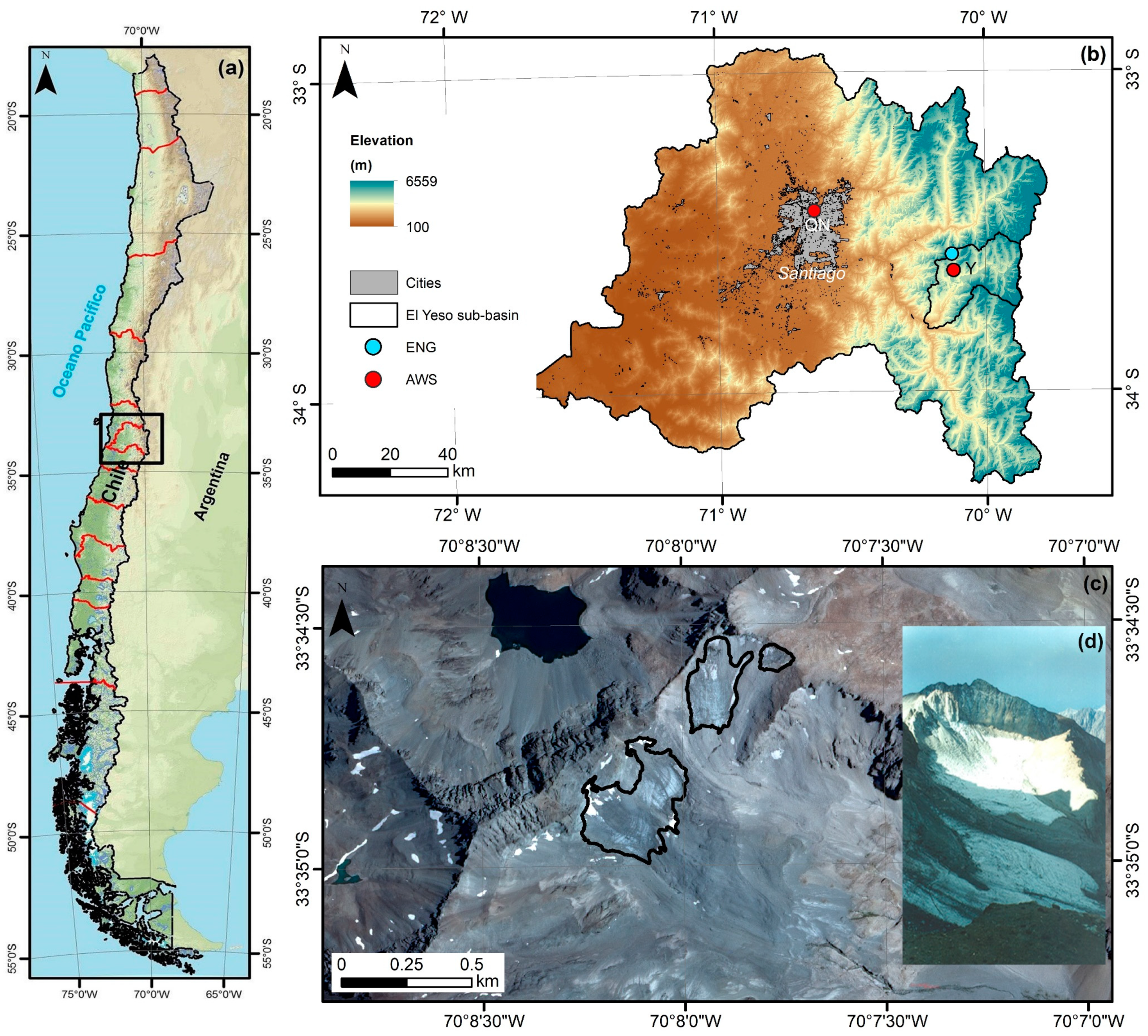
2. Study Area
3. Materials and Methods
3.1. Glacier Area Changes
3.2. Geodetic Mass Balance and Volume Changes
3.3. Accuracy and Uncertainties
4. Results
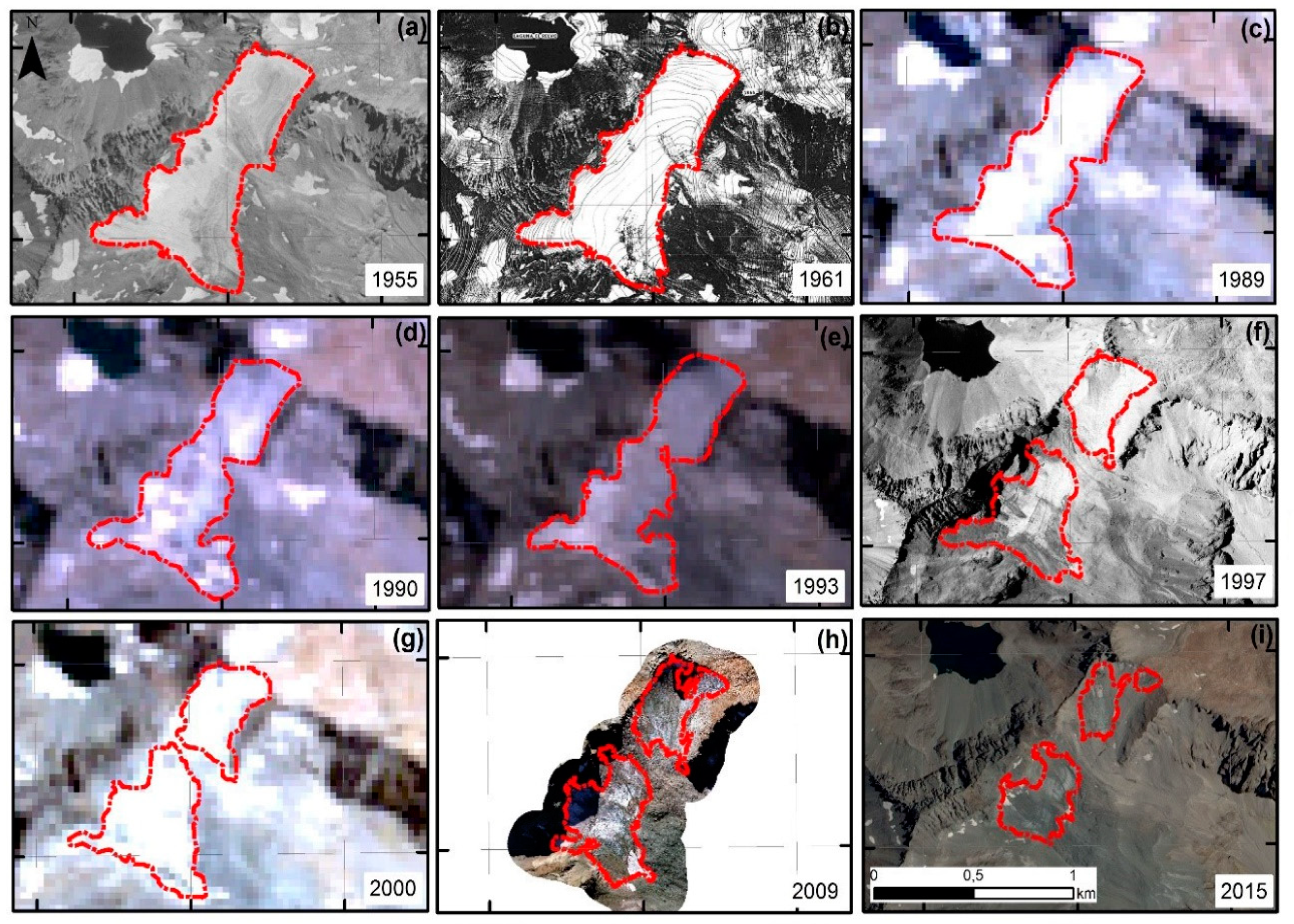
4.1. Area Change
4.2. Glacier Mass Balance and Volume Change
5. Discussion
5.1. Comparison with Other Studies
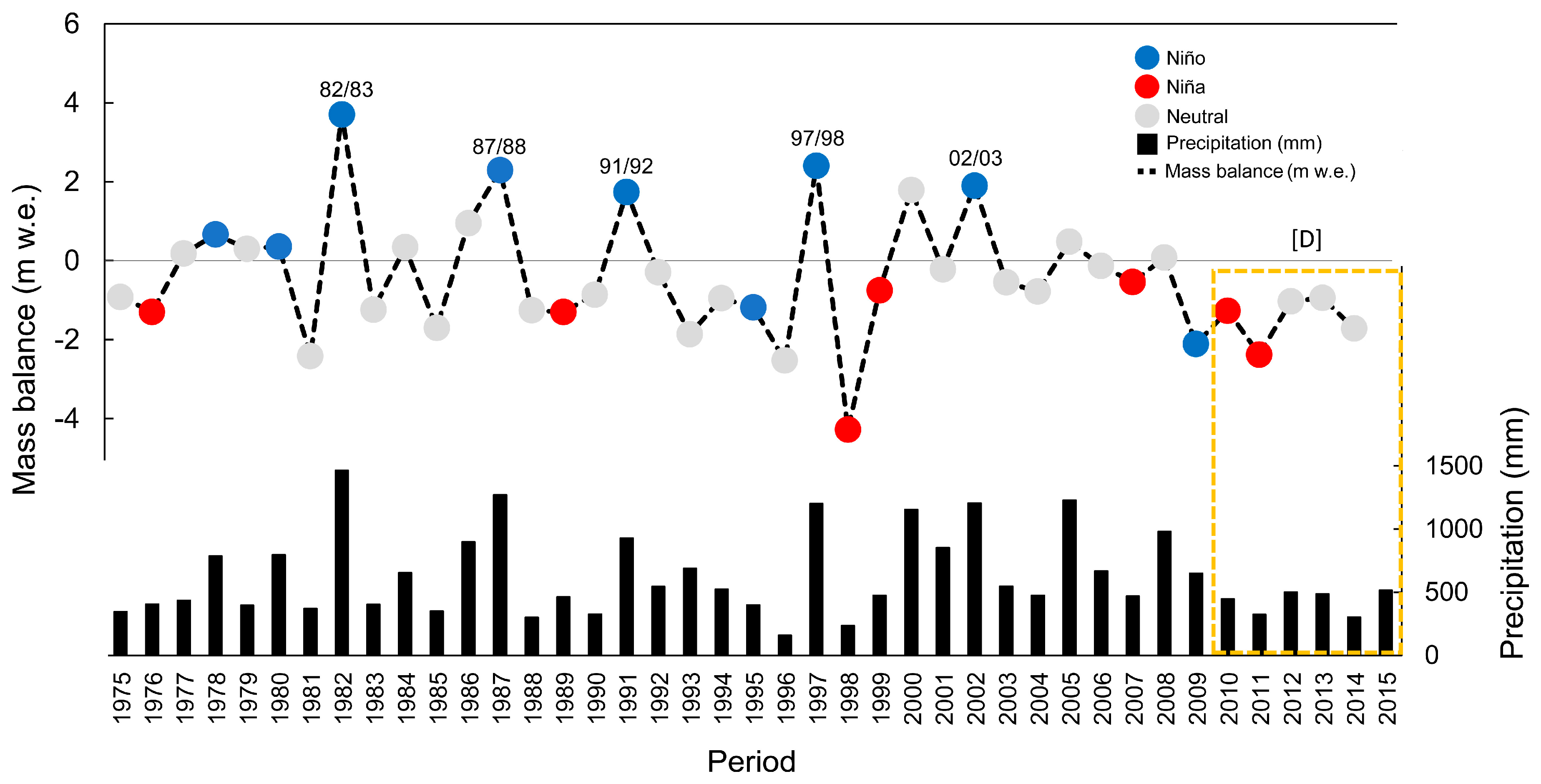
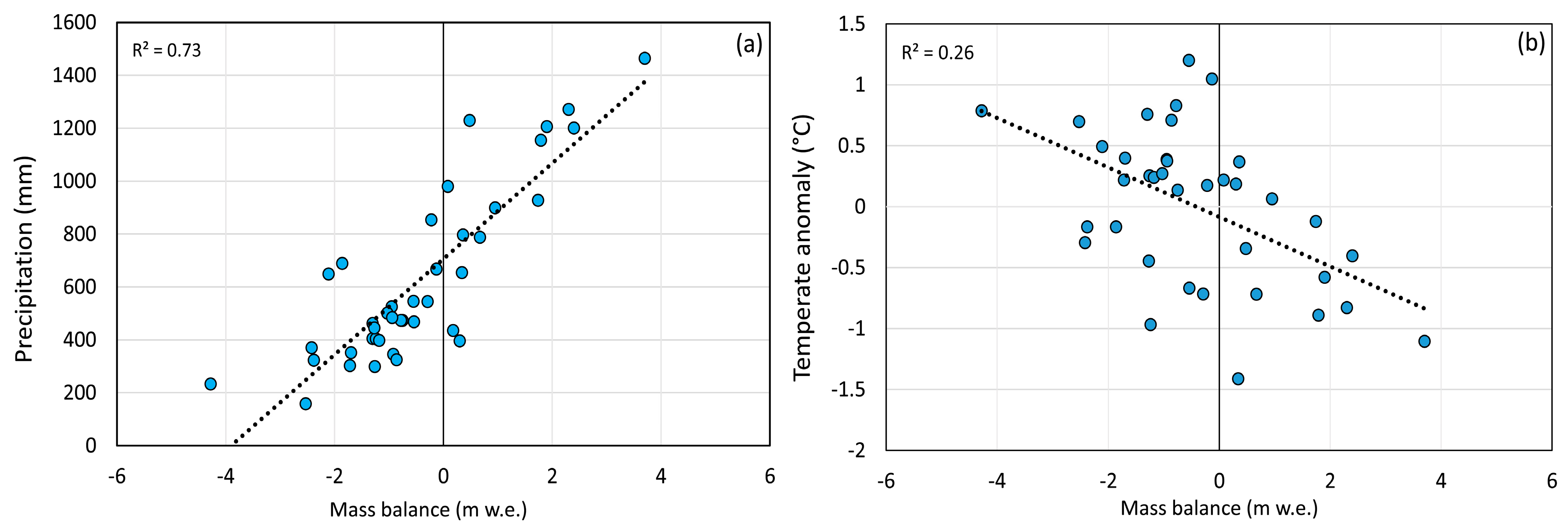
5.2. Climatic Trends at Maipo Basin
6. Conclusions
Supplementary Materials
Author Contributions
Funding
Acknowledgments
Conflicts of Interest
References
- WGMS. Global Glacier Change Bulletin No. 2 (2014–2015); Zemp, M., Nussbaumer, S.U., Gärtner Roer, I., Huber, J., Machguth, H., Paul, F., Hoelzle, M., Eds.; ICSU(WDS)/IUGG(IACS)/UNEP/UNESCO/WMO; World Glacier Monitoring Service: Zurich, Switzerland, 2017; 244p. [Google Scholar] [CrossRef]
- Casassa, G.; Haeberli, W.; Jones, G.; Kaser, G.; Ribstein, P.; Rivera, A.; Schneider, C. Current status of Andean glaciers. Glob. Planet. Chang. 2007, 59, 1–9. [Google Scholar] [CrossRef]
- Vaughan, D.G.; Allison, I.; Carrasco, J.; Kaser, G.; Kwok, R.; Mote, P.; Murray, T.; Paul, F.; Ren, J.; Rignot, E.; et al. Observations: Cryosphere. In Climate Change 2013: The Physical Science Basis; Contribution of Working Group I to the Fifth Assessment Report of the Intergovernmental Panel on Climate Change; Stocker, T.F., Qin, D., Plattner, G.K., Tignor, M., Allen, S.K., Boschung, J., Nauels, A., Xia, Y., Bex, V., Midgley, P.M., Eds.; Cambridge University Press: Cambridge, UK; New York, NY, USA, 2013. [Google Scholar]
- Oerlemans, J.; Reichert, B.K. Relating glacier mass balance to meteorological data by using a seasonal sensitivity characteristic. J. Glaciol. 2000, 46, 1–6. [Google Scholar] [CrossRef]
- Kaser, G.; Cogley, J.G.; Dyurgerov, M.B.; Meier, M.F.; Ohmura, A. Mass balance of glaciers and ice caps: Consensus estimates for 1961–2004. Geophys. Res. Lett. 2006, 33, L19501. [Google Scholar] [CrossRef]
- Kaltenborn, B.P.; Muhammed, A.; Lamadrid, A.; Benn, D.; Kaser, G.; Paul, F.; Koboltschnig, G.; Casassa, G.; Reynolds, J.M.; Hagen, J.O.; et al. High Mountain Glaciers and Climate Change: Challenges to Human Livelihoods and Adaptation; Nellemann, V., II, Ed.; United Nations Environment Programme; Birkeland Trykkeri AS: Birkeland, Norway, 2010; ISBN 978-82-7701-087. [Google Scholar]
- Zemp, M.; Frey, H.; Gärtner-Roer, I.; Nussbaumer, S.U.; Hoelzle, M.; Paul, F.; Haeberli, W.; Denzinger, F.; Ahlstrøm, A.P.; Anderson, B.; et al. Historically unprecedented global glacier decline in the early 21st century. J. Glaciol. 2015, 61, 745–762. [Google Scholar] [CrossRef] [Green Version]
- Montecinos, A.; Aceituno, P. Seasonality of the ENSO-related rainfall variability in central Chile and associated circulation anomalies. J. Clim. 2003, 16, 281–296. [Google Scholar] [CrossRef]
- Masiokas, M.; Villalba, R.; Luckman, B.; LeQuesne, C.; Aravena, J.C. Snowpack variations in the central Andes of Argentina and Chile, 1951–2005: Large-scale atmospheric influences and implications for water resources in the region. J. Clim. 2006, 19, 6334–6352. [Google Scholar] [CrossRef]
- Garreaud, R. Warm winter storms in Central Chile. J. Hydrometeorol. 2013, 14, 1515–1534. [Google Scholar] [CrossRef]
- Boisier, J.P.; Rondanelli, R.; Garreaud, R.; Muñoz, F. Anthropogenic and natural contributions to the Southeast Pacific precipitation decline and recent megadrought in central Chile. Geophys. Res. Lett. 2016, 43, 413–421. [Google Scholar] [CrossRef] [Green Version]
- Garreaud, R.; Alvarez-Garreton, C.; Barichivich, J.; Boisier, J.P.; Christie, D.; Galleguillos, M.; LeQuesne, C.; McPhee, J.; Zambrano-Bigiarini, M. The 2010–2015 mega drought in Central Chile: Impacts on regional hydroclimate and vegetation. Hydrol. Earth Syst. Sci. 2017, 21, 6307–6327. [Google Scholar] [CrossRef]
- Falvey, M.; Garreaud, R. Regional cooling in a warming world: Recent temperature trends in the southeast Pacific and along the west coast of subtropical South America (1979–2006). J. Geophys. Res. 2009, 114, D04102. [Google Scholar] [CrossRef]
- Carrasco, J.; Casassa, G.; Quintana, J. Changes of the 0 °C isotherm and equilibrium line altitude in central Chile during the last quarter of the 20th Century. Hydrol. Sci. J. 2005, 50, 933–948. [Google Scholar] [CrossRef]
- Carrasco, J.F.; Osorio, R.; Casassa, G. Secular trend of the equilibrium-line altitude on the western side of the southern Andes, derived from radiosonde and surface observations. J. Glaciol. 2008, 54, 538–550. [Google Scholar] [CrossRef]
- Le Quesne, C.; Acuña, C.; Boninsegna, J.A.; Rivera, A.; Barichivich, J. Long-term glacier variations in the Central Andes of Argentina and Chile, inferred from historical records and tree ring reconstructed precipitation. Palaeogeogr. Palaeoclimatol. Palaeoecol. 2009, 281, 334–344. [Google Scholar] [CrossRef]
- Malmros, J.K.; Mernild, S.H.; Wilson, R.; Fensholt, R.; Yde, J.C. Glacier area changes in the central Chilean and Argentinean Andes 1955–2013/2014. J. Glaciol. 2016, 62, 391–401. [Google Scholar] [CrossRef]
- Valdés-Pineda, R.; Pizarro, R.; Valdés, J.B.; Carrasco, J.F.; García-Chevesich, P. Spatio-temporal trends of precipitation, its aggressiveness and concentration, along the Pacific coast of South America (36°–49°S). Hydrol. Sci. J. 2015, 61, 2110–2132. [Google Scholar] [CrossRef]
- Rosegrant, M.W.; Ringler, C.; McKinney, D.C.; Cai, X.; Keller, A.; Donoso, G. Integrated economic-hydrologic water modeling at the basin scale: The Maipo river basin. Agric. Econ. 2000, 24, 33–46. [Google Scholar]
- Peña, H.; Nazarala, B. Snowmelt-runoff simulation model of a central Chile Andean basin with relevant orographic effects. In Symposium at Vancouver 1987—Large Scale Effects of Seasonal Snow Cover; IAHS Publisher: Vancouver, BC, Canada, 1987; Volume 166, pp. 161–172. [Google Scholar]
- Casassa, G.; Apey, A.; Bustamante, M.; Maragunic, C.; Salazar, C.; Soza, D. Contribución hídrica de glaciares en el estero Yerba Loca y su extrapolación a la cuenca del río Maipo. In Proceedings of the XIV Congreso Geológico Chileno, La Serena, Chile, 4–8 October 2015. [Google Scholar]
- Ayala, A.; Pellicciotti, F.; MacDonell, S.; McPhee, J.; Vivero, S.; Campos, C.; Egli, P. Modelling the hydrological response of debris-free and debris-covered glaciers to present climatic conditions in the semiarid Andes of central Chile. Hydrol. Processes 2016, 30, 4036–4058. [Google Scholar] [CrossRef]
- Rabatel, A.; Castebrunet, H.; Favier, V.; Nicholson, L.; Kinnard, C. Glacier changes in the Pascua-Lama region, Chilean Andes (29 S): Recent mass balance and 50 yr surface area variations. Cryosphere 2011, 5, 1029–1041. [Google Scholar] [CrossRef]
- Escobar, F.; Casassa, G.; Pozo, V. Variaciones de un glaciar de montaña en los Andes de Chile central en las últimas dos décadas. Bulletin de l’Institut Français d’Etudes Andines 1955, 24, 683–695. [Google Scholar]
- Schaefer, M.; Rodriguez, J.; Scheiter, M.; Casassa, G. Climate and surface mass balance of Mocho Glacier, Chilean Lake District, 40°S. J. Glaciol. 2017, 63, 218–228. [Google Scholar] [CrossRef]
- Willis, M.J.; Melkonian, A.K.; Pritchard, M.E.; Ramage, J.M. Ice Loss Rates at the Northern Patagonian Icefield Derived Using a Decade of Satellite Remote Sensing. Remote Sens. Environ. 2012, 117, 184–198. [Google Scholar] [CrossRef]
- Ginot, P.; Kull, C.; Schotterer, U.; Schwikowski, M.; Gäggeler, H.W. Glacier mass balances reconstruction by sublimation induced enrichment of chemical species on Cerro Tapado (Chilean Andes). Clim. Past 2006, 2, 21–30. [Google Scholar] [CrossRef]
- Matsuoka, K.; Naruse, R. Mass balance features derived from a firn core at Hielo Patagonico Norte, South America. Arct. Antarct. Alp. Res. 1999, 31, 333–340. [Google Scholar]
- Shiraiwa, T.; Kohshoma, S.; Uemura, R.; Yoshida, N.; Matoba, S.; Uetake, J.; Godoi, M.A. High net accumulation rates at Campo de Hielo Patagónico Sur, South America revealed by analysis of a 45.97 m long ice core. Ann. Glaciol. 2002, 35, 84–90. [Google Scholar] [CrossRef]
- Schaefer, M.; Machguth, H.; Falvey, M.; Casassa, G.; Rignot, E. Quantifying mass balance processes on the Southern Patagonia Icefield. Cryosphere 2015, 9, 25–35. [Google Scholar] [CrossRef] [Green Version]
- Merlind, S.H.; Liston, G.; Hiemstra, C.; Wilson, R. The Andes Cordillera. Part III: Glacier surface mass balance and contribution to sea level rise (1979–2014). J. Clim. 2016, 37, 3154–3174. [Google Scholar]
- Casassa, G.; Rivera, A.; Schwikowski, M. Glacier mass-balance data for southern South America (30°S–56°S). In Glacier Science and Environmental Change; Knight, P., Ed.; Blackwell: Oxford, UK, 2006; pp. 239–241. [Google Scholar]
- Masiokas, M.H.; Christie, D.A.; Le Quesne, C.; Pitte, P.; Ruiz, L.; Villalba, R.; Luckman, B.H.; Berthier, E.; Nussbaumer, S.U.; González-Reyes, A.; et al. Reconstructing the annual mass balance of the Echaurren Norte glacier (Central Andes, 33.5° S) using local and regional hydroclimatic data. Cryosphere 2016, 10, 927–940. [Google Scholar] [CrossRef] [Green Version]
- Meza, F.J.; Wilks, D.; Gurovich, L.; Bambach, N. Impacts of Climate Change on Irrigated Agriculture in the Maipo Basin, Chile: Reliability of Water Rights and Changes in the Demand for Irrigation. J. Water Res. Plan. Manag. 2012, 138, 421–430. [Google Scholar] [CrossRef]
- Østrem, G.; Brugman, M. Glacier Mass-Balance Measurements: A Manual for Field and Office Work; NHRI Science Report; Arctic Institute of North America: Saskatoon, SK, Canada, 1991. [Google Scholar]
- Mayo, L.; Meier, M.; Tangborn, W. A system to combine stratigraphic and annual mass-balance systems: A contribution to the International Hydrological Decade. J. Glaciol. 1972, 11, 3–14. [Google Scholar] [CrossRef]
- Cogley, J.G.; Hock, R.; Rasmussen, L.A.; Arendt, A.A.; Bauder, A.; Braithwaite, R.J.; Jansson, P.; Kaser, G.; Möller, M.; Nicholson, L.; et al. Glossary of Glacier Mass Balance and Related Terms; IHP-VII Technical Documents in Hydrology, No. 86, IACS Contribution No. 2; UNESCO-IHP: Paris, France, 2011. [Google Scholar]
- Peña, H.; Vidal, F.; Escobar, F. Caracterización del manto nival y mediciones de ablación y balance de masa en Glaciar Echaurren Norte. In Jornadas de Hidrología de Nieves y Hielos en América del Sur; Santiago de Chile, United Nations Educational, Scientific, and Cultural Organization, International Hydrology Programme: Santiago, Chile, 1984; pp. 1–12. [Google Scholar]
- DGA. Balance de Masa del Glaciar Echaurren Norte Temporadas 1997–98 a 2008–2009; Technical Report; Fernando Escobar and Cristobal Cox: Santiago, Chile, 2010. [Google Scholar]
- Mikhail, E.M.; Bethel, J.S.; McGlone, J.C. Introduction to Modern Photogrammetry; John Wiley and Sons Inc.: New York, NY, USA, 2001. [Google Scholar]
- DGA. Modelo Digital de Elevación de Centros Montañosos y Glaciares de las Zonas Glaciológicas Norte y Centro, Mediante LiDAR Aerotranpsortado; Technical Report; Digimapas: Santiago, Chile, 2015. [Google Scholar]
- Paul, F.; Kääb, A.; Maisch, M.; Kellenberger, T.W.; Haeberli, W. The new remote-sensing-derived Swiss glacier inventory: I. Methods. Ann. Glaciol. 2002, 34, 355–361. [Google Scholar] [CrossRef] [Green Version]
- Paul, F.; Huggel, C.; Kääb, A. Combining satellite multispectral image data and a digital elevation model for mapping debris-covered glaciers. Remote Sens. Environ. 2004, 89, 510–518. [Google Scholar] [CrossRef]
- Paul, F.; Barrand, N.E.; Baumann, S.; Berthier, E.; Bolch, T.; Casey, K.; Frey, H.; Joshi, S.P.; Konovalov, V.; Bris, R.L.; et al. On the accuracy of glacier outlines derived from remote-sensing data. Ann. Glaciol. 2013, 54, 171–182. [Google Scholar] [CrossRef] [Green Version]
- Williams, R.; Hall, D.; Sigurosson, O.; Chien, Y. Comparison of satellite-derived with ground-based measurements of the fluctuations of themargins of Vatnajökull, Iceland, 1973–1992. Ann. Glaciol. 1997, 24, 72–80. [Google Scholar] [CrossRef]
- Mölg, N.; Ceballos, J.L.; Huggel, C.; Micheletti, N.; Rabatel, A.; Zemp, M. Ten years of monthly mass balance of Conejeras glacier, Colombia, and their evaluation using different interpolation methods. Geogr. Ann. Ser. A Phys. Geogr. 2017, 99, 155–176. [Google Scholar] [CrossRef]
- Farr, T.G.; Rosen, P.; Caro, E.; Crippen, R.; Duren, R.; Hensley, S.; Kobrick, M.; Paller, M.; Rodriguez, E.; Roth, L.; et al. The Shuttle Radar Topography Mission. Rev. Geophys. 2007, 45, RG2004. [Google Scholar] [CrossRef]
- Hoffmann, J.; Walter, D. How complementary are SRTM-X and-C band digital elevation models? Photogramm. Eng. Remote Sens. 2006, 72, 261–268. [Google Scholar] [CrossRef]
- Rankl, M.; Braun, M. Glacier elevation and mass changes over the central Karakoram region estimated from TanDEM-X and SRTM/X-SAR digital elevation models. Ann. Glaciol. 2016, 57, 273–281. [Google Scholar] [CrossRef] [Green Version]
- Seehaus, T.; Marinsek, S.; Helm, V.; Skvarca, P.; Braun, M. Changes in ice dynamics, elevation and mass discharge of Dinsmoor-Bombardier-Edgeworth glacier system, Antarctic Peninsula. Earth Planet. Sci. Lett. 2015, 427, 125–135. [Google Scholar] [CrossRef]
- Goldstein, R.M.; Werner, C.L. Radar interferogram filtering for geophysical applications. Geophys. Res. Lett. 1998, 25, 4035–4038. [Google Scholar] [CrossRef] [Green Version]
- Costantini, M. A novel phase unwrapping method based on network programming. IEEE Trans. Geosci. Remote Sens. 1998, 36, 813–821. [Google Scholar] [CrossRef]
- Malz, P.; Meier, E.; Casassa, G.; Jaña, R.; Svarca, P.; Braun, M. Elevation and mass changes of the Southern Patagonia Icefield derived from TanDEM-X and SRTM data. Remote Sens. 2018, 10, 188. [Google Scholar] [CrossRef]
- DGA. Levantamiento Topográfico Láser Aerotransportado para los Glaciares Echaurren Norte y San Francisco; Technical Report; Terra Remote Sensing Inc.: Sidney, BC, Canada, 2009. [Google Scholar]
- Nuth, C.; Kääb, A. Co-registration and bias corrections of satellite elevation data sets for quantifying glacier thickness change. Cryosphere 2011, 5, 271–290. [Google Scholar] [CrossRef] [Green Version]
- Huss, M. Density assumptions for converting geodetic glacier volume change to mass change. Cryosphere 2013, 7, 877–887. [Google Scholar] [CrossRef] [Green Version]
- Jaber, W.A.; Floricioiu, D.; Rott, H.; Eineder, M. Surface elevation changes of glaciers derived from SRTM and TanDEM-X DEM differences. In Proceedings of the 2013 IEEE International Geoscience and Remote Sensing Symposium (IGARSS), Melbourne, Australia, 21–26 July 2013; pp. 1893–1896. [Google Scholar]
- Falaschi, D.; Bolch, T.; Rastner, P.; Lenzano, M.; Lenzano, L.; Lo Vecchio, A.; Moragues, S. Mass changes of alpine glaciers at the eastern margin of the Northern and Southern Patagonian Icefields between 2000 and 2012. J. Glaciol. 2017, 63, 258–272. [Google Scholar] [CrossRef]
- Ruiz, L.; Berthier, E.; Viale, M.; Pitte, P.; Masiokas, M.H. Recent geodetic mass balance of Monte Tronador glaciers, northern Patagonian Andes. Cryosphere 2017, 11, 619–634. [Google Scholar] [CrossRef] [Green Version]
- Rivera, A.; Casassa, G.; Acuña, C.; Lange, H. Variaciones recientes de glaciares en Chile. Investig. Geogr. 2000, 34, 29–60. [Google Scholar] [CrossRef]
- Leiva, J.; Cabrera, G.; Lenzano, L. 20 years of mass balances on the Piloto glacier, Las Cuevas river basin, Mendoza, Argentina. Glob. Planet. Chang. 2007, 59, 10–16. [Google Scholar] [CrossRef]
- Barcaza, G.; Segovia, A.; Farías, D.; Huenante, J.; Vergara, A.; Gonzalez, D.; Varela, B. Surface elevation change of Andean glaciers in Central Chile, based upon airborne laser altimetry and ground-truth GPS measurements (Abstract 5649). In Proceedings of the 26th International Union Geodesy and Geophysics General Assembly, Prague, Czech Republic, 22 June–2 July 2015. [Google Scholar]
- Zemp, M.; Thibert, E.; Huss, M.; Stumm, D.; Rolstad Denby, C.; Nuth, C.; Nussbaumer, S.U.; Moholdt, G.; Mercer, A.; Mayer, C.; et al. Reanalysing glacier mass balance measurement series. Cryosphere 2013, 7, 1227–1245. [Google Scholar] [CrossRef] [Green Version]
- Garreud, R.D.; Vuille, M.; Compagnucci, R.; Marengo, J. Present-day South American climate. Palaeogeogr. Palaeoclimatol. Palaeoecol. 2009, 281, 180–195. [Google Scholar] [CrossRef]
- Burger, F.; Brock, B.; Montecinos, A. Seasonal and elevation contrasts in temperature trends in Central Chile between 1979 and 2015. Glob. Planet. Chang. 2018, 162, 136–147. [Google Scholar] [CrossRef]
- Quintana, J.M.; Aceituno, P. Changes in the rainfall regime along the extratropical west coast of South America (Chile): 30–43° S. Atmosfera 2012, 25, 1–22. [Google Scholar]
- Herreid, S.; Pellicciotti, F.; Ayala, A.; Chesnokova, A.; Kienholz, C.; Shea, J.; Shrestha, A. Satellite observations show no net change in the percentage of supraglacial debris-covered area in northern Pakistan from 1977 to 2014. J. Glaciol. 2015, 61, 524–536. [Google Scholar] [CrossRef] [Green Version]
- Huss, M.; Fischer, M. Sensitivity of Very Small Glaciers in the Swiss Alps to Future Climate Change. Front. Earth Sci. 2016, 4, 34. [Google Scholar] [CrossRef]
- Fischer, M.; Huss, M.; Barboux, C.; Hoelzle, M. The new Swiss Glacier Inventory SGI2010: Relevance of using high-resolution source data in areas dominated by very small glaciers. Arct. Antarct. Alp. Res. 2014, 46, 933–945. [Google Scholar] [CrossRef]
- DeBeer, C.M.; Sharp, M.J. Topographic influences on recent changes of very small glaciers in the Monashee Mountains, British Columbia, Canada. J. Glaciol. 2009, 55, 691–700. [Google Scholar] [CrossRef]
- Ramírez, E.; Francou, B.; Ribstein, P.; Descloitres, M.; Guérin, R.; Mendoza, J.; Gallaire, R.; Pouyaud, B.; Jordan, E. Small glaciers disappearing in the tropical Andes: A case-study in Bolivia: Glaciar Chacaltaya (16° S). J. Glaciol. 2001, 47, 187–194. [Google Scholar] [CrossRef]
- Berger, T.; Mendoza, J.; Francou, B.; Rojas, F.; Fuertes, R.; Flores, M.; Noriega, L.; Rammalo, C.; Ramirez, E. Glaciares Zongo—Chacaltaya—Charquini Sur. Bolivia 16°S. Mediciones Glaciológicas, Hidrológicas y Meteorológicas, Año Hidrológico 2004–2005; IRDIHH-SENMAHI-COBEE; Informe Great Ice Bolivia: Bolivia, 2005; p. 171. [Google Scholar]


| Date | Survey | Spatial Resolution | Source |
|---|---|---|---|
| 24 February 1955 | HYCON aerial photos | 1 m | IGM |
| 1961 | OEA aerial photos | 1 m | IGM/SAF |
| 02 March 1989 | Landsat TM satellite image | 30 m | USGS |
| 05 March 1990 | Landsat TM satellite image | 30 m | USGS |
| 29 March 1993 | Landsat TM satellite image | 30 m | USGS |
| March 1997 | GEOTEC aerial photos | 1 m | SAF |
| 20 February 2000 * | Landsat TM satellite image | 30 m | USGS |
| 28 April 2009 | DGA LiDAR orthophoto | 0.2 m | DGA |
| 30 January 2015 | SPOT satellite image | 1.5 m | DGA |
| Year | Sensor/Products | Nominal Scale/Spatial Resolution | Source |
|---|---|---|---|
| 24 February 1955 | Aerial Camera/Chilean topographic maps | 1:50,000 | IGM |
| 11–22 February 2000 | SRTM C-band | 30 m | USGS/NASA |
| 28 April 2009 | LiDAR (Mark II) | 1 m | DGA/Terra RSL |
| 27 January 2013 | TanDEM-X | 30 m | DLR |
| 23 February 2015 | LiDAR (Harrier 68i) | 1 m | DGA/Digimapas |
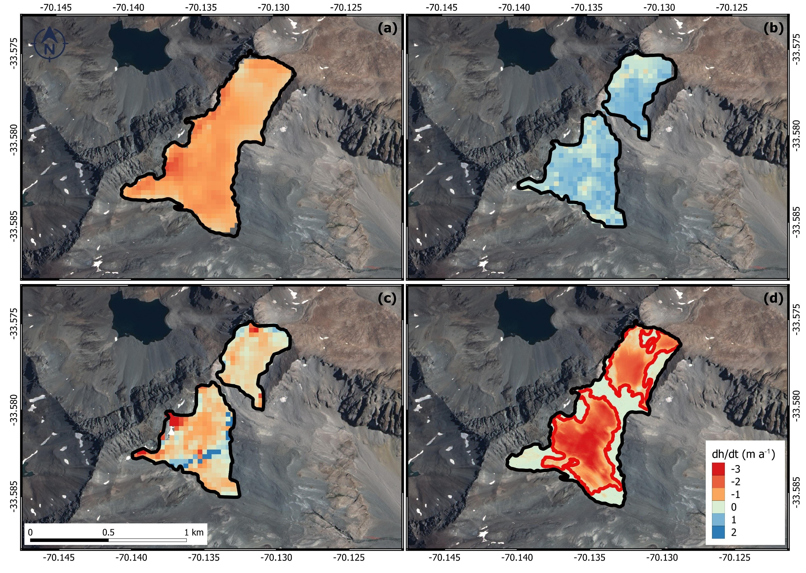
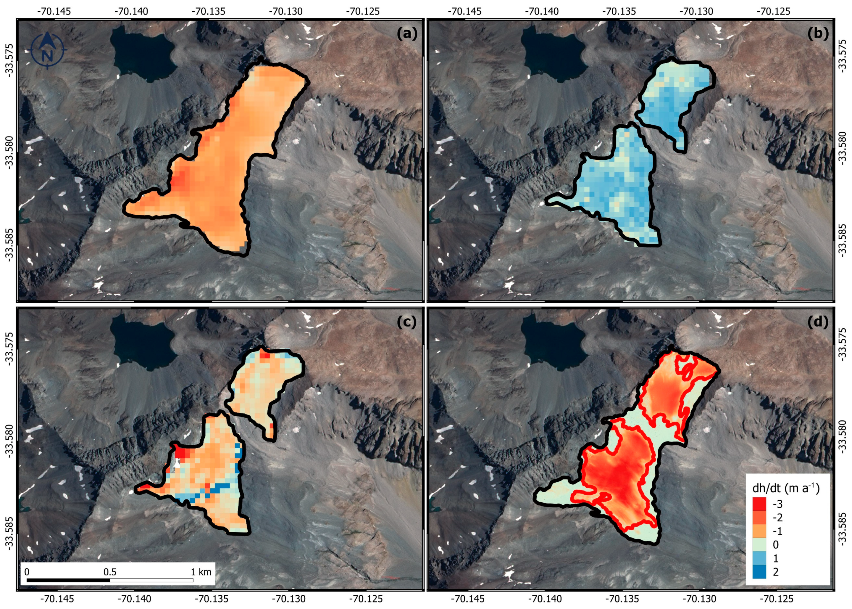
| Period | Volume Change (km3) | Geodetic Mass Balance (m w.e.) | Geodetic Mass Balance (m w.e. a−1) |
|---|---|---|---|
| 1955–2000 | −0.0220 ± 0.0010 | −38.29 ± 3.72 | −0.85 ± 0.08 |
| 2000–2009 | 0.0020 ± 0.0010 | 4.87 ± 3.59 | 0.54 ± 0.40 |
| 2000–2013 | −0.0020 ± 0.0005 | −4.64 ± 1.10 | −0.36 ± 0.09 |
| 2009–2015 | −0.0020 ± 0.0001 | −7.21 ± 0.57 | −1.20 ± 0.09 |
© 2019 by the authors. Licensee MDPI, Basel, Switzerland. This article is an open access article distributed under the terms and conditions of the Creative Commons Attribution (CC BY) license (http://creativecommons.org/licenses/by/4.0/).
Share and Cite
Farías-Barahona, D.; Vivero, S.; Casassa, G.; Schaefer, M.; Burger, F.; Seehaus, T.; Iribarren-Anacona, P.; Escobar, F.; Braun, M.H. Geodetic Mass Balances and Area Changes of Echaurren Norte Glacier (Central Andes, Chile) between 1955 and 2015. Remote Sens. 2019, 11, 260. https://doi.org/10.3390/rs11030260
Farías-Barahona D, Vivero S, Casassa G, Schaefer M, Burger F, Seehaus T, Iribarren-Anacona P, Escobar F, Braun MH. Geodetic Mass Balances and Area Changes of Echaurren Norte Glacier (Central Andes, Chile) between 1955 and 2015. Remote Sensing. 2019; 11(3):260. https://doi.org/10.3390/rs11030260
Chicago/Turabian StyleFarías-Barahona, David, Sebastián Vivero, Gino Casassa, Marius Schaefer, Flavia Burger, Thorsten Seehaus, Pablo Iribarren-Anacona, Fernando Escobar, and Matthias H. Braun. 2019. "Geodetic Mass Balances and Area Changes of Echaurren Norte Glacier (Central Andes, Chile) between 1955 and 2015" Remote Sensing 11, no. 3: 260. https://doi.org/10.3390/rs11030260